Semi-Self Representation Learning for Crowdsourced WiFi Trajectories
Abstract
WiFi fingerprint-based localization has been studied intensively. Point-based solutions rely on position annotations of WiFi fingerprints. Trajectory-based solutions, however, require end-position annotations of WiFi trajectories, where a WiFi trajectory is a multivariate time series of signal features. A trajectory dataset is much larger than a pointwise dataset as the number of potential trajectories in a field may grow exponentially with respect to the size of the field. This work presents a semi-self representation learning solution, where a large dataset of crowdsourced unlabeled WiFi trajectories can be automatically labeled by a much smaller dataset of labeled WiFi trajectories. The size of only needs to be proportional to the size of the physical field, while the unlabeled could be much larger. This is made possible through a novel “cut-and-flip” augmentation scheme based on the meet-in-the-middle paradigm. A two-stage learning consisting of trajectory embedding followed by endpoint embedding is proposed for the unlabeled . Then the learned representations are labeled by and connected to a neural-based localization network. The result, while delivering promising accuracy, significantly relieves the burden of human annotations for trajectory-based localization.
Keywords: Constrastive Learning, Crowdsourcing, Deep Learning, Indoor Localization, Representation Learning.
I Introduction
Location-based service (LBS) is essential in smart city, smart driving, and tour guiding applications. The core of LBS is localization. Indoor localization techniques can be divided into three categories: geometrical positioning, pedestrian dead-reckoning (PDR), and fingerprint matching [1]. Geometric approaches may be derived by triangulation, angle of arrival, and time difference of arrival of specific wireless signals. PDR does not require auxiliary signals, but only measures relative motions and thus may suffer from accumulative errors. Fingerprint-matching approaches require annotated fingerprint datasets [2, 3], but acquiring the datasets is costly.
This work focuses on fingerprint-based solutions. While fingerprints collection by humans or robots is easy, assigning labels to fingerprints is laborious and error-prone. To address this issue, [4] uses robots for automatic data and label collection. Inpainting and interpolation are addressed in [5]. With the popularity of mobile devices, crowdsourcing is promising for data collection. However, such data are typically unlabeled and even unreliable. A framework for evaluating crowdsourced data quality is in [6]. Estimating WiFi APs’ propagation parameters with crowdsourcing is explored in [7], and a crowdsourcing-based SLAM mechanism for radio map construction is explored in [8]. Using crowdsourced data effectively in the deep learning domain remains a challenge.
WiFi-based localization can be either point-based (using a single fingerprint) or trajectory-based (using a sequence of fingerprints). This paper focuses on learning representations from WiFi trajectories, modeled as multivariate time series along roaming paths. We assume access to two datasets: a large unlabeled, crowdsourced set , and a smaller labeled set , with to reduce annotation effort. Our semi-self-supervised framework learns representations from in an unsupervised manner, then uses to assign pseudo-labels to . We show that combining and improves localization accuracy, provided is sufficiently large and scales with the field size.
The kernel of our design is a “cut-and-flip” augmentation scheme following the meet-in-the-middle paradigm. Specifically, given a long trajectory, if we cut it in the middle and flip the second half, then the resulting two sub-trajectories should meet in the middle position, meaning that their endpoint embeddings should be very close to each other. If we repeat the same process many times, a lot of sub-trajectories shall meet in the same middle position, and if any one of these sub-trajectories appears in , all these trajectories will have an opportunity to converge to very similar embeddings. Therefore, those pseudo-labels would become meaningful, making localization possible. Following this, we separate our learning into trajectory embedding and endpoint embedding. With the assistance of , we can attain a higher localization accuracy. The results significantly reduce human annotation efforts.
In the literature, self-supervised learning (SSL) is proposed to extract intrinsic insights from data without labels. Predictive SSL makes a success in natural language processing [9, 10, 11, 12, 13]. Siamese networks use negative pairs [14, 15]), while others use positive pairs only (e.g., BYOL [16], SimSiam [17] and SwAV [18]). Our framework will utilize positive pairs only because negative pairs are difficult to define and wireless signals in indoor environments may fluctuate significantly, resulting in numerous similar fingerprints for a location [19].
Our method is presented in Section II. Section III shows our experiment results. Section IV concludes this work.
II Semi-Self Representation Learning
We are given a dataset containing a large number of crowdsourced WiFi trajectories that are unlabeled. A WiFi trajectory is a multivariate time series , where is the total number of observable WiFi APs, is the sequence length, and represents the features of the th AP at the th position in the trajectory, , . On the other hand, a very small labeled dataset is given, . Each WiFi trajectory in is accompanied by a position label in , representing its end position.
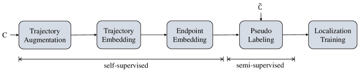
Our semi-self representation learning consists of two parts. The representation learning of the trajectories in is completely unsupervised. Then we assign pseudo labels to by utilizing the labels in . The learning workflow is shown in Fig. 1. Trajectory augmentation first transforms the samples in into more samples, which are regarded as positive samples. Trajectory embedding and endpoint embedding then compute each trajectory’s representation in a self-supervised manner. After pseudo labeling, the combined can be used for a localization task.
II-A Trajectory Augmentation
To deal with signal fluctuation, we design four ways to augment a WiFi trajectory for representation learning. Given a trajectory , we augment it to multiple , regarded as positive samples of .
-
1.
Flipping: This operation swaps on the temporal axis into .
-
2.
Additive: To model signal fluctuation, a small is added to a randomly sampled , resulting in the augmented sequence , where controls the noise magnitude.
-
3.
Scaling: Randomly sampled is scaled by a factor of , where and is a tunable parameter, resulting in .
-
4.
Masking: To model intermittent WiFi signals, a short randomly sampled segment is regarded missing, where and is a small integer. These missing signals are filled by the last or previously available signal or . Note that multiple segments of can be masked to obtain .
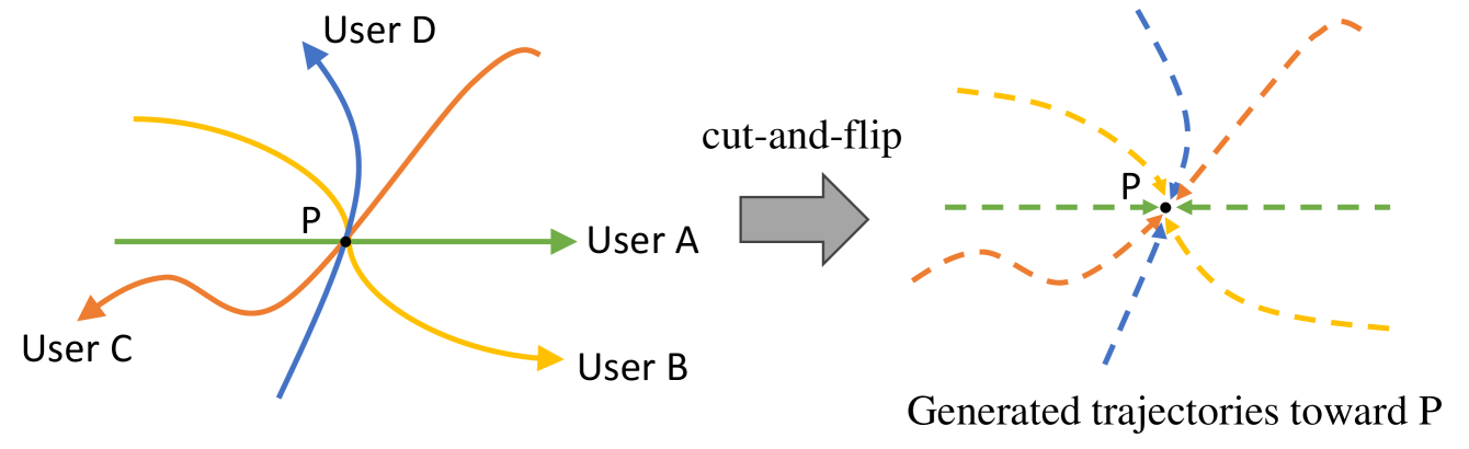
In addition, we propose a new “meet-in-the-middle” paradigm to explore self representation learning. The augmentation is called Cut-and-Flip. Consider a length- sequence in . We first cut it in the middle, resulting in two sequences and . We then flip along the temporal axis, resulting in . Intuitively, if a person walks along and another person walks along , they will meet in the same position (middle). That is, and can be regarded as a positive pair, in terms of their end positions. In Fig. 2, we show an intersection point where many pedestrians pass through. All segments of the trajectory ending at and all segments of the trajectory departing from , after flipped, can be regarded as positive samples. Therefore, when sufficient crowdsourced trajectories are collected, it is possible to self-learn similar representations from them without human annotations. This paradigm empowers crowdsourced WiFi trajectories to be used in localization tasks even if they are unlabeled.
II-B Two-Stage Representation Learning
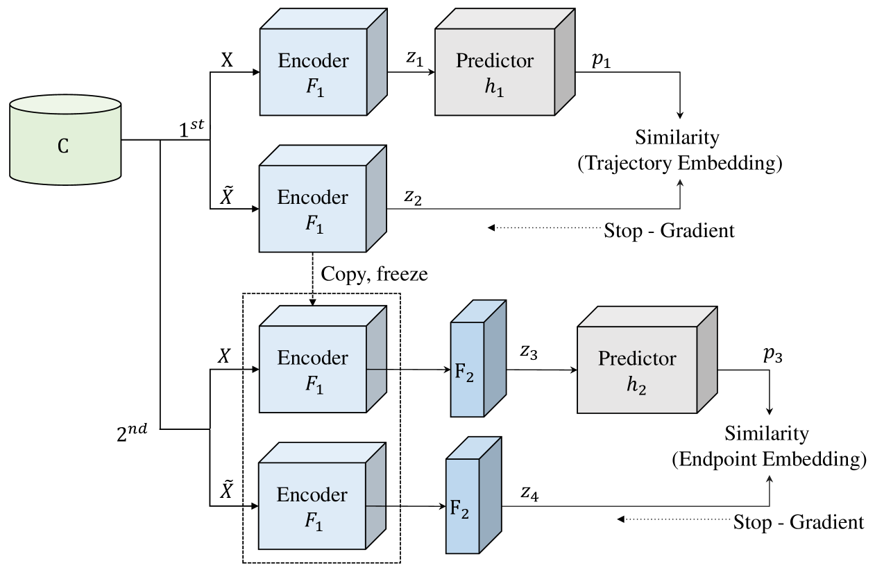
With augmented positive pairs, we can perform representation learning. There are two stages: (i) The trajectory embedding will utilize pairs augmented by flipping, additive, scaling, and masking. (ii) The endpoint embedding will utilize pairs produced by cut-and-flip. There are different frameworks for self-representation learning. As our WiFi trajectories’ endpoints fall in a continuous physical space, negative pairs are hard to define. Hence, we choose to use SimSiam [17], which requires positive pairs only. The learning framework is shown in Fig. 3, which has two pairs of Siamese networks.
II-B1 Trajectory Embedding
The upper part of Fig. 3 is to learn the characteristics of WiFi trajectories. Given a trajectory and its augmentation , we consider them as a positive pair. Both and go through the encoder network and the predictor .
| (1) |
We swap the roles of and and compute two negative cosine similarities:
| (2) |
| (3) |
To avoid model collapse, stop-gradient (SG) is introduced. The loss function is defined as:
| (4) |
The process is totally self-supervised. After finishing training, is frozen and used in the next stage.
II-B2 Endpoint Embedding
The lower part of Fig. 3 is to learn the characteristics of the end positions of the WiFi trajectories. It has similar Siamese networks with a frozen copied from the first stage to maintain trajectory characteristics. Additional encoder and predictor are inserted. Given and its augmentation (from cut-and-flip), we also consider them as a positive pair. Through , , and , we obtain:
| (5) | ||||
The similarity and loss functions are defined similarly. The embedding of the endpoint is written as .
II-C Pseudo Labeling
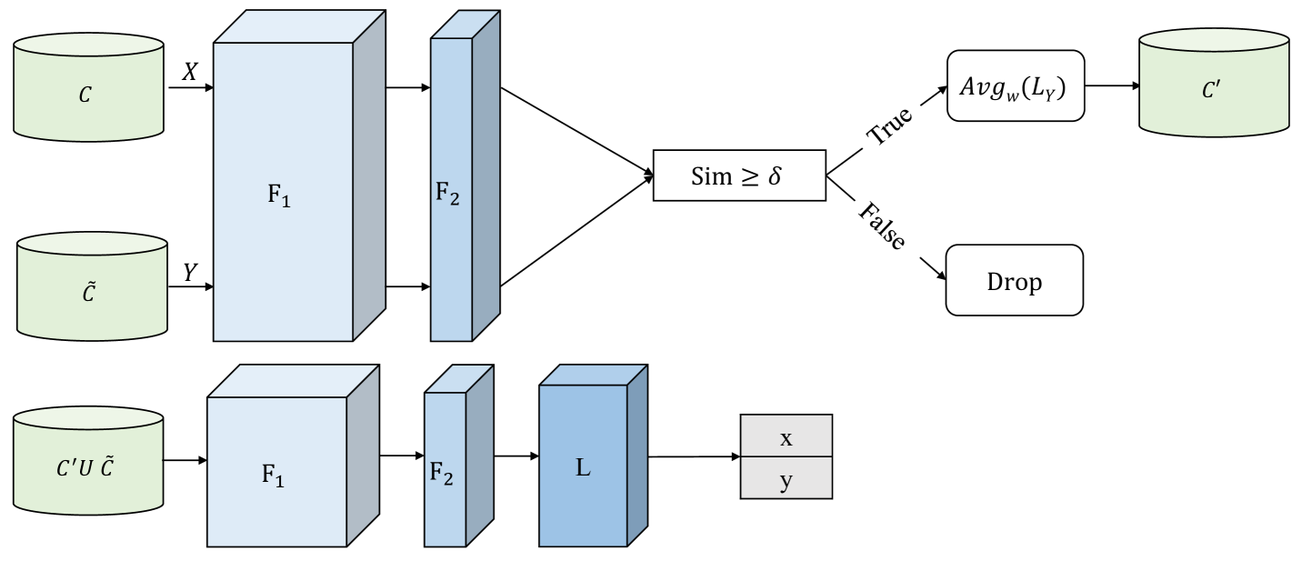
With endpoint representations, we can conduct pseudo labeling on with the assistance of . The workflow is shown in Fig. 4. For each , we compute its embedding and compare it against for each . If their cosine similarity is above a threshold , the label of is considered a candidate. If there are multiple candidates, a weighted average of these labels, , is regarded as ’s label; otherwise, will be dropped. The refined dataset is named .
II-D Localization Training
The size of the annotated set only needs to be proportional to the field size. However, the number of possible trajectories with respect to a filed may grow exponentially, making the crowdsourced set much larger than . Therefore, the pseudo-labeled set is potentially large too.
We use the labels of the union to train a localization model, which is composed of , , and a mapping network , as shown in Fig. 4. and help to find a WiFi trajectory’s embedding that is unique to a position. Then maps the embedding to a position . A lot of previous work has addressed the design of , so we omit the details.
III Experiment Results
III-A Datasets
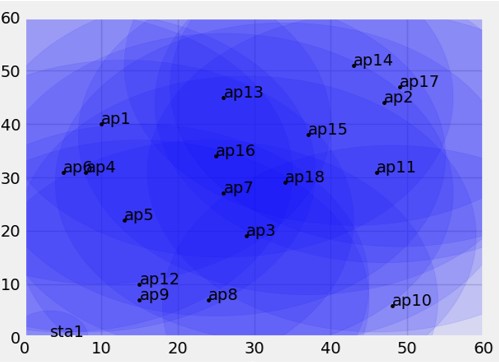
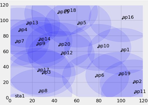
To validate our claims, we construct two WiFi trajectory datasets using the emulation tool Mininet-WiFi [20, 21]. As illustrated in Fig. 5, we simulate two environments: Field 1 and Field 2, with dimensions of m x m and m × m, respectively. Each field contains 18 and 20 randomly deployed access points (APs), respectively. The RSSI values are collected based on the log-normal shadowing propagation model. The path loss at a distance meters is determined by:
| (6) |
where is the path loss at a reference distance , is the environment-dependent path loss exponent (set to ), and is a zero-mean Gaussian random variable representing shadowing effects, with standard deviation . The maximum transmission range is set to . RSSI values are sampled on a 2D grid with m spacing between adjacent points.
| learning rate | 0.01 |
| initial decay epochs | 100 |
| min decay learning rate | 0.0001 |
| restart interval | 30 |
| restart learning rate | 0.001 |
| warmup epochs | 40 |
| warmup start learning rate | 0.001 |

To simulate human movement, we generate trajectories in and by connecting grid points using the Levywalk model [22], with speeds between – m/s. Each trajectory lasts seconds with 1-second intervals, yielding 15-point sequences. RSSI at each point is from its nearest grid location. We generate M trajectories for the and K labeled trajectories for in both fields. All RSSI values are distorted with noise and normalized to .
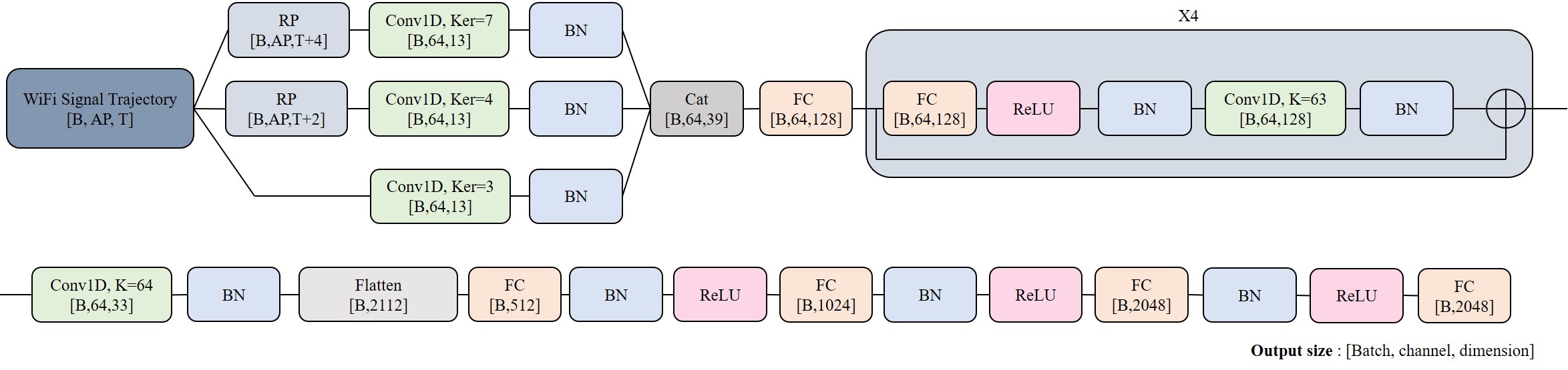
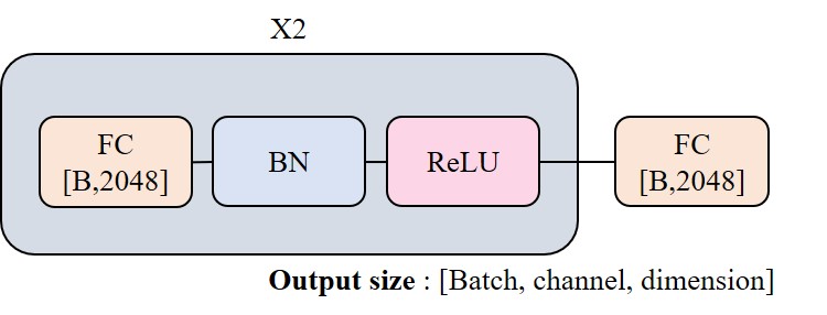
III-B Model Specifications
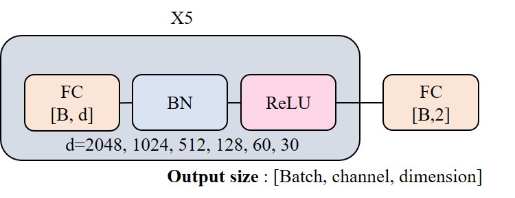
Our model consists of a trajectory encoder , an endpoint encoder , two predictors (, ), and a localization module , as shown in Fig. 6. All components follow a projection-based architecture with 1D convolutions, batch normalization, ReLU activations, and fully connected (FC) layers. For first-stage trajectory augmentation, we apply the following configurations: (1) Additive: , (2) Scaling: , (3) Masking: masked segment length (20–60% of each trajectory). We train using SGD with a cyclic cosine decay schedule (in Table 5) on an NVIDIA RTX 3090. After freezing , we train using the same settings and then train with the Adam optimizer.
III-C Ablation Study
III-C1 1-to-1 Embedding Distance
Given two crowdsourced trajectories and with the same endpoint, let and be their trajectory embeddings from the first-stage encoder , and and be their endpoint embeddings from the second-stage encoder . Let and denote the similarities between the respective pairs. Since both trajectories converge at the same endpoint, we expect .
In Field 1, this condition holds in of cases. Among them, show a minor improvement (), and show a significant improvement (). In the remaining (), most already have high similarity where fall within , and only fall below 0.7. Field 2 shows a similar trend, though the portion of is lower, likely due to reduced WiFi AP density. Nevertheless, only of non-improving cases fall below the threshold. These results validate the effectiveness of our two-stage framework.
|
|
CDF68 | CDF95 | |||||
|
0.8 | 0.7% | 3.19 | 6.58 | ||||
| 0.9 | 9.8% | 2.84 | 5.39 | |||||
|
0.8 | 0.01% | 2.91 | 6.36 | ||||
| 0.9 | 3.3% | 2.45 | 4.93 | |||||
|
0.8 | 0.2% | 10.0 | 20.85 | ||||
| 0.9 | 3.8% | 8.35 | 18.12 | |||||
|
0.8 | 0% | 9.68 | 20.35 | ||||
| 0.9 | 1.2% | 7.69 | 17.36 |
| Model | KNN | LSTM | NCP | FULL | ||||||
| Crowdsourced | 0 | 0 | 0 | 0 | 10k | 200k | 10k | 200k | 10k | 200k |
| Threshold | - | - | - | - | 0.8 | 0.9 | 0.99 | |||
| Training dataset size | 0.5k | 0.6k | 0.5k | 0.5k | 10.5k | 199.8k | 9.6k | 181.2k | 1.4k | 9.8k |
| Position error CDF68 | 7.81 | 7.16 | 8.37 | 6.7 | 5.77 | 4.7 | 5.34 | 4.16 | 5.97 | 11.21 |
| Position error CDF95 | 16.27 | 13.14 | 16.97 | 13.1 | 10.01 | 8.17 | 8.61 | 7.28 | 9.63 | 20.06 |
| Model | KNN | LSTM | NCP | FULL | ||||||
| Crowdsourced | 0 | 0 | 0 | 0 | 10k | 200k | 10k | 200k | 10k | 200k |
| Threshold | - | - | - | - | 0.8 | 0.9 | 0.99 | |||
| Training dataset size | 0.5k | 0.5k | 0.5k | 0.5k | 10.5k | 199.8k | 9.6k | 193.2k | 1.4k | 57.5k |
| Position error CDF68 | 22.95 | 18.47 | 59.19 | 57.81 | 14.98 | 11.53 | 13.34 | 10.32 | 18.64 | 20.3 |
| Position error CDF95 | 61.32 | 35.84 | 77.63 | 75.83 | 23.44 | 21.69 | 22.21 | 19.64 | 37.37 | 38.15 |
III-C2 Accuracy of Pseudo Labels
With effective trajectory and endpoint embeddings, we exploit a small labeled set to assign pseudo labels to the larger crowdsourced dataset , using a similarity threshold . Note that the endpoints in are evenly distributed. Table II reports the results for Field 1. With 1K labeled samples and , the localization errors are m (CDF68) and m (CDF95), with of trajectories left unlabeled. Reducing the threshold to increases errors to m and m, respectively, but nearly all trajectories are labeled (only dropped). This suggests that label quality matters more than quantity, and a higher threshold yields more accurate pseudo labels.
Using only 0.5K labeled samples, we observe the same trend: yields better accuracy than across both CDF68 and CDF95. However, overall performance declines compared to the 1K case, indicating that while quality is critical, quantity still plays a supporting role. Field 2 exhibits similar patterns, but with degraded accuracy due to its larger area and sparser AP density.
III-C3 Effectiveness of the Two-Stage Design
We evaluate the two-stage framework against an endpoint-only baseline (only cut-and-flip augmentation) that skips trajectory embedding and directly learns endpoint representations. As shown in Table II, the two-stage model achieves a strong localization accuracy with 0.5K labeled samples, which is m (CDF68) and m (CDF95) in . In contrast, the endpoint-only model performs poorly regardless of threshold, with errors exceeding m (CDF68) and m (CDF95) in both and . These results highlight the importance of trajectory-level embedding. Without it, the model fails to capture discriminative movement patterns, leading to large localization errors.
III-D Comparisons
We compare our method against several baselines: (i) KNN, (ii) LSTM trained on the labeled set , (iii) NCP, our architecture without pretraining and without using , and (iv) FULL, our complete model. Only FULL takes advantage of the unlabeled crowd-sourced dataset through pseudo labeling.
Table III shows results in field 1 using K. Even without , our FULL model, with pretraining on , achieves better accuracy than LSTM and NCP (e.g., m CDF68 vs. m and m). Adding 10K pseudo-labeled samples from improves accuracy to m (CDF68), and up to m with 200K samples. Varying controls the quality–quantity trade-off where produces the best result, while limits usable data and degrades accuracy.
The results in field 2 (Table IV) show larger errors due to lower label density and sparser AP coverage. However, the trend remains consistent where pseudo-labeled data from substantially improve localization. Optimal performance is achieved again with .
IV Conclusions
We have proposed a two-stage semi-self supervised training for learning representations of unlabeled crowdsourced data. Separating trajectory embedding and endpoint embedding has been proved helpful in predicting the endpoint of a WiFi trajectory. A novel cut-and-flip mechanism is proposed to self-learn the representations of unlabeled crowdsourced trajectories. The framework has been tested on small-scale datasets. The results could greatly reduce laborious data labeling costs. Future work can be directed to more extensive tests and the next-generation WiFi technologies.
Acknowledgement: Y.-C. Tseng’s research was sponsored by NSTC grants 113-2639-E-A49-001-ASP and 113-2634-F-A49-004.
References
- [1] Y. Li, Z. He, Z. Gao, Y. Zhuang, C. Shi, and N. El-Sheimy, “Toward robust crowdsourcing-based localization: A fingerprinting accuracy indicator enhanced wireless/magnetic/inertial integration approach,” IEEE Internet of Things J., vol. 6, no. 2, pp. 3585–3600, 2019.
- [2] A. Poulose and D. S. Han, “Hybrid deep learning model based indoor positioning using Wi-Fi RSSI heat maps for autonomous applications,” MDPI Electronics, vol. 10, no. 1, 2021.
- [3] R. Ayyalasomayajula, A. Arun, C. Wu, S. Sharma, A. R. Sethi, D. Vasisht, and D. Bharadia, “Deep learning based wireless localization for indoor navigation,” in ACM MobiCom, 2020.
- [4] Y. Peng, X. Niu, J. Tang, D. Mao, and C. Qian, “Fast signals of opportunity fingerprint database maintenance with autonomous unmanned ground vehicle for indoor positioning,” MDPI Sensors, vol. 18, no. 10, 2018.
- [5] M. Nabati, H. Navidan, R. Shahbazian, S. A. Ghorashi, and D. Windridge, “Using synthetic data to enhance the accuracy of fingerprint-based localization: A deep learning approach,” IEEE Sensors Lett., vol. 4, no. 4, pp. 1–4, 2020.
- [6] P. Zhang, R. Chen, Y. Li, X. Niu, L. Wang, M. Li, and Y. Pan, “A localization database establishment method based on crowdsourcing inertial sensor data and quality assessment criteria,” IEEE Internet of Things J., vol. 5, no. 6, pp. 4764–4777, 2018.
- [7] Y. Zhuang, Y. Li, H. Lan, Z. Syed, and N. El-Sheimy, “Smartphone-based WiFi access point localisation and propagation parameter estimation using crowdsourcing,” IET Electronic. Lett., vol. 51, no. 17, pp. 1380–1382.
- [8] J. Yang, C.-K. Wen, S. Jin, and X. Li, “Enabling plug-and-play and crowdsourcing SLAM in wireless communication systems,” IEEE Trans. Wireless Commun., vol. PP, pp. 1–1, 08 2021.
- [9] J. Devlin, M.-W. Chang, K. Lee, and K. Toutanova, “BERT: Pre-training of deep bidirectional transformers for language understanding,” in Assoc. for Computational Linguistics Conf.: Human Language Technologies, Vol. 1, Jun. 2019, pp. 4171–4186.
- [10] T. Brown, B. Mann, N. Ryder, M. Subbiah, J. D. Kaplan, P. Dhariwal, and et al., “Language models are few-shot learners,” in NIPS, vol. 33, 2020, pp. 1877–1901.
- [11] A. Radford, J. Wu, R. Child, D. Luan, D. Amodei, I. Sutskever et al., “Language models are unsupervised multitask learners,” OpenAI blog, vol. 1, no. 8, p. 9, 2019.
- [12] M. E. Peters, M. Neumann, M. Iyyer, M. Gardner, C. Clark, K. Lee, and L. Zettlemoyer, “Deep contextualized word representations,” in Assoc. for Computational Linguistics Conf.: Human Language Technologies, Vol. 1, Jun. 2018.
- [13] A. Vaswani, N. Shazeer, N. Parmar, J. Uszkoreit, L. Jones, A. N. Gomez, L. u. Kaiser, and I. Polosukhin, “Attention is all you need,” in NIPS, vol. 30, 2017.
- [14] T. Chen, S. Kornblith, M. Norouzi, and G. Hinton, “A simple framework for contrastive learning of visual representations,” in ICML, 2020.
- [15] K. He, H. Fan, Y. Wu, S. Xie, and R. Girshick, “Momentum contrast for unsupervised visual representation learning,” in IEEE CVPR, 2020.
- [16] J.-B. Grill, F. Strub, F. Altché, C. Tallec, P. H. Richemond, E. Buchatskaya, C. Doersch, B. A. Pires, Z. D. Guo, M. G. Azar, B. Piot, K. Kavukcuoglu, R. Munos, and M. Valko, “Bootstrap your own latent a new approach to self-supervised learning,” in NIPS, 2020.
- [17] X. Chen and K. He, “Exploring simple siamese representation learning,” in IEEE CVPR, 2021, pp. 15 750–15 758.
- [18] M. Caron, I. Misra, J. Mairal, P. Goyal, P. Bojanowski, and A. Joulin, “Unsupervised learning of visual features by contrasting cluster assignments,” in NIPS, vol. 33, 2020, pp. 9912–9924.
- [19] Y.-T. Liu, J.-J. Chen, Y.-C. Tseng, and F. Y. Li, “An auto-encoder multitask LSTM model for boundary localization,” IEEE Sensors J, vol. 22, no. 11, pp. 10 940–10 953, 2022.
- [20] R. d. R. Fontes and C. E. Rothenberg, “Mininet-WiFi: A platform for hybrid physical-virtual software-defined wireless networking research,” in ACM SIG COMM, 2016, p. 607–608.
- [21] R. R. Fontes, S. Afzal, S. H. B. Brito, M. A. S. Santos, and C. E. Rothenberg, “Mininet-WiFi: Emulating software-defined wireless networks,” in IEEE CNSM, 2015, pp. 384–389.
- [22] I. Rhee, M. Shin, S. Hong, K. Lee, S. J. Kim, and S. Chong, “On the levy-walk nature of human mobility,” IEEE/ACM Transactions Networking, vol. 19, no. 3, pp. 630–643, 2011.