Fluctuation-dissipation of the Kuramoto model on fruit-fly connectomes

Abstract

We investigate the distance from equilibrium using the Kuramoto model via the degree of fluctuation-dissipation violation as the consequence of different levels of edge weight anisotropies. This is achieved by solving the synchronization equations on the raw, homeostatic weighted and a random inhibitory edge variant of a real full fly (FF) connectome, containing $\simeq 10^{5}$ neuron cell nodes. We investigate these systems close to their synchronization transition critical points. While the topological(graph) dimension is high: $d\simeq 6$ the spectral dimensions of the variants, relevant in describing the synchronization behavior, are lower than the upper critical dimension: $d_{s}\simeq 2<d_{c}=4$, suggesting relevant fluctuation effects and non mean-field scaling behavior. By measuring the auto-correlations and the auto-response functions for small perturbations we calculate the fluctuation-dissipation ratios (FDR) for the different variants of different anisotropy levels of the FF connectome. Numerical evidence is presented that the FDRs follow the level of anisotropy of these non-equilibrium systems in agreement with the expectations. We also compare these results with those on a symmetric random graph of similar size. We provide a detailed network analysis of the FF connectome and calculate the level of hierarchy, also related to the anisotropy. Finally, we provide some partial results for the periodic forced Kuramoto, the Shinomoto-Kuramoto model.

Introduction

Non-equilibrium systems can be characterized by the violation of the fluctuation-dissipation (vFD) relation [1, 2]. Very recently the vFD in neural systems has been studied by [3, 4] and the relation between vFD and the asymmetry of the interactions has been demonstrated using empirical human neuroimaging data as well as whole-brain models.

Far-from-equilibrium systems often display dynamical scaling, even if the stationary state is very far from being critical [5, 6]. Criticality, often occurring at continuous, second-order phase transitions, is common in nature and beneficial for systems. In neural systems, criticality allows for the generation of working memory, spontaneous long-range interactions, and maximal sensitivity to external signals due to diverging correlations and fluctuations [7, 8, 9]. Information-processing is also optimal near the critical point [10, 11, 12, 8], leading systems to self-organize close to criticality (SOC) [13, 11], or slightly below it to avoid over-excitation. This can also happen in the dynamical, semi-critical so called Griffiths phase [14, 15, 16, 17, 18].

Another important, open question is the topology and the level of anisotropy of neural systems. The modular structure of brain is well known, but whether they follow hierarchical or non-hierarchical organization is debated. To fill this gap we determined the modules of the largest exactly known brain, the full fruit fly connectome by community detecting algorithm and run an up to date anisotropy measuring method, based on directed random walk approach. In this work we investigate the relation of anisotropy and non-equilibrium critical dynamical behavior within the framework of this connectome, using an oscillatory model for the function.

Here summarize in nutshell the fluctuation-dissipation (FD) theory through the relation between the response and the auto-correlation functions. The auto-response function $\mathcal{R}(t,s)$ of an observable $E(t)$ of the system to a small enough perturbation $h$ at time $s$ is given by

$$\mathcal{R}(t,s)=\frac{\delta E_{h}(t,s)}{\delta h}|_{h}\to 0\ ,$$ (1)

whereas the auto-correlation between the start $s$ and measurement $t$ times is defined as

$$A(t,s)=\langle E(t)E(s)\rangle,$$ (2)

here $\langle\cdot\rangle$ states for the ensemble average. At the critical point $A(s,t)$ and $\mathcal{R}(s,t)$ are expected to decay asymptotically in the $t\to\infty$ limit with power-law (PL) tails, which for non-equilibrium systems scale as

$$\mathcal{R}(t/s)\propto s^{-1-a}(t/s)^{-\lambda_{\mathcal{R}}/Z}$$ (3)

$$A(t/s)\propto s^{-b}(t/s)^{-\lambda_{A}/Z}\ ,$$ (4)

where $t\gg s$, $Z$ is the dynamical, $\lambda_{\mathcal{R}}$ is the auto-response, $\lambda_{A}$ is the auto-correlation exponents and $b$, $a$ are the so called aging exponents [5].

The FD theory states that, if a system is in equilibrium, the response function is related to the auto-correlation function of the unperturbed observable by

$$\mathcal{R}(t,s)=\frac{1}{T}\frac{\partial A(t,s)}{\partial s},$$ (5)

where $s<t$, and $T$ is the temperature of the thermal bath. However, if the system is out of equilibrium a way to measure the difference from equilibrium, is through the FD ratio

$$\mathcal{R}(t,s)=\frac{1}{T}X(t,s)\frac{\partial A(t,s)}{\partial s},\$$ (6)

where $\frac{1}{T}X(t,s):=\mathrm{FDR}$ characterizes the distance from equilibrium. If $\lim_{(t/s)\to\infty}X(t,s)=1$, the system is in equilibrium with temperature $T$. Conversely, a non-equilibrium system can be characterized by the deviation of FDR from a constant value. In sections (“Auto-correlation results”), (“Auto-response results”) we calculate this ratio in case of different modifications of the largest currently known connectome, the structural network of a fruit-fly for different levels of re-weighting of the edges, corresponding to different brain states. These states exhibit different levels of anisotropies. Before that we provide network analysis of the the structural connectome and define it’s states, realizing different levels of edges weights corresponding to operation of excitatory and inhibitory mechanisms (“Asymmetry in the interactions”). Following that we introduce the brain toy model. the Shinomoto-Kuramoto equation (“The Shinomoto-Kuramoto model with external force”) we used to model the synchronization mechanism of the oscillatory behavior and determine its critical points for each scenario (“Synchronization transition point results”).

Results

Topology of the full fruit-fly connectome (FF)

Communities

The $Q$ value, characterizing modularity (see Methods) is not independent of the community detection method. If our detection method produces lower modularity than the maximum achieved, it means our algorithm has fallen behind others. Community detection algorithms based on modularity optimization will get the closest to the actual modular properties of the network. We calculated and compared the modularity quotients, using community structures of the FF and the hemibrain (HB) [33], by the Louvain method [19]. The results for these networks are: $Q_{HB}\approx 0.631$, $Q_{FF}\approx 0.6466$, similar to each other despite all the differences and very far from the highly modular ($Q\approx 0.91$–$0.92$) human connetomes.

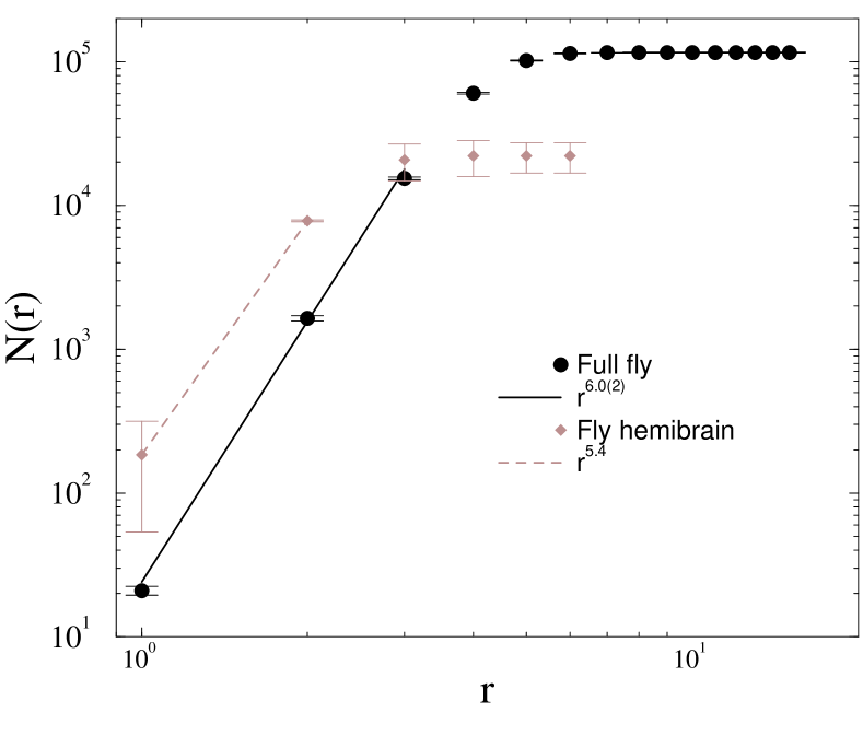
Figure 1: Comparison of the topological dimension measurements of the FF and the hemibrain. Lines show to least square Pl fits, with exponents corresponding to the topological (graph) dimensional estimates.

The FF connectome (v630) [20], obtained from a different fruit-fly species than that of the HB, contains $N_{FF}=124891$ nodes and $L_{FF}=3794615$ edges, out of which the largest single connected component has $N_{FF}=115661$ nodes and $L_{FF}=3719871$ links. Note that the FF connectome is 5 times bigger, yet the number of links that connect them is not that much larger. This results an average node degree of $\langle k\rangle=64.323$ (for the in-degrees it is: $32.161$), the average weighted degree is $\langle w_{FF}\rangle=557.241$. Similarly, to the HB for the FF we found PL tailed global weight distributions characterized by the exponent: $-3.0(1)$, even if glia cells are filtered out. On the other hand the in/out degree (local, weight) distributions can be better fitted via log-normal distributions [21].

Graph (topological) dimension

These measurements are explained in the Section Methods. Note, that finite size cutoff happens very early. Fig. 1 shows the comparison of dimensions, obtained for the hemi-brain (HB) and the full-fly (FF). While we can estimate $d\simeq 5.4$ for the HB, for the FF a somewhat larger dimension: $d\simeq 6.0(2)$ can be obtained. These dimensions suggest the fly connectomes to belong to the mean-field critical behavior, as the upper-critical dimension is $d_{c}=4$ in case of the Kuramoto model [22] and the higher dimensional FF graph. However, the above statement was shown in case of regular, finite dimensional lattices [23, 24].

Asymmetry of the FF connectome variants

To characterize the global graph anisotropy of the edge weight modified versions of the FF we introduced a measure in Sect. Methods, which provides the following values of $a$ of the scenarios as:

• $a=0.163$, for the original FF (o)

• $a=0.1$, for case (i), with $20\%$ random negative weights

• $a=2\times 10^{-5}$, for the renormalized weighs case (w)

In this study we shall compare the dynamical behavior of the Kuramoto model on these networks versions.

Spectral dimension

As Eqs. (10) and (11) hold for small $\lambda$ values, for the fruit-fly connectome with which $N\gg 1$, we extract the densities for the first 1200 smallest eigenvalues for ease of eigenvalue computation without loss of generality. With this method the $d_{s}$ of the HB connectome has already been estimated in [25] and $d^{o}_{s}=3.37$, for the original, $d^{w}_{s}=2.34$, for the weighted dimensions were obtained. The full FF connectome contains $N_{ff}=124.891$ nodes, requiring large computational efforts, therefore, we used the thick-restart Lanczos [26] with sparse matrix representation and accelerated with graphics processing unit (GPU), using the latest version (13.4.0) of the CuPy extension. As we can see on Fig. 2 for (o) and (i) we get $d^{o}_{s}=2.082$, $d^{i}_{s}=2.831$ respectively, within error margins of the log-log fitting, while for (w) a larger value, similarly to HB case, $d^{w}_{s}=2.156$ is obtained. Important to note that these dimensions are smaller than the $d_{c}=4$ threshold of the mean-field behavior [27], thus we may expect different dynamical scaling of the Kuramoto model at the synchronization transition.

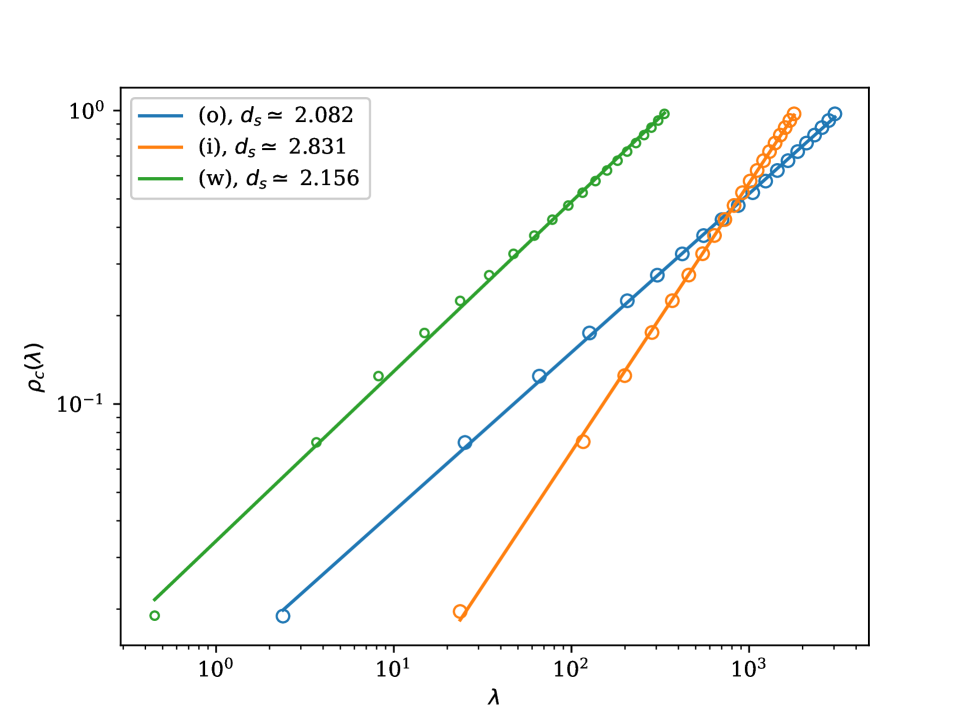
Figure 2: Lowest Laplacian eigenvalues of the Full Fly connectomes for edge weight scenarios (o), (i), (w). The straight lines are PL fittings for the smallest eigenvalues with exponents shown by the legends.

Graph hierarchy

We can see on Fig.3 that the FF communities are larger than the literature reference ones, but their hierarchy value $H$ is somewhat smaller. This result also contributes to the debate whether brain networks are hierarchical modular (HMN) or just simply modular.

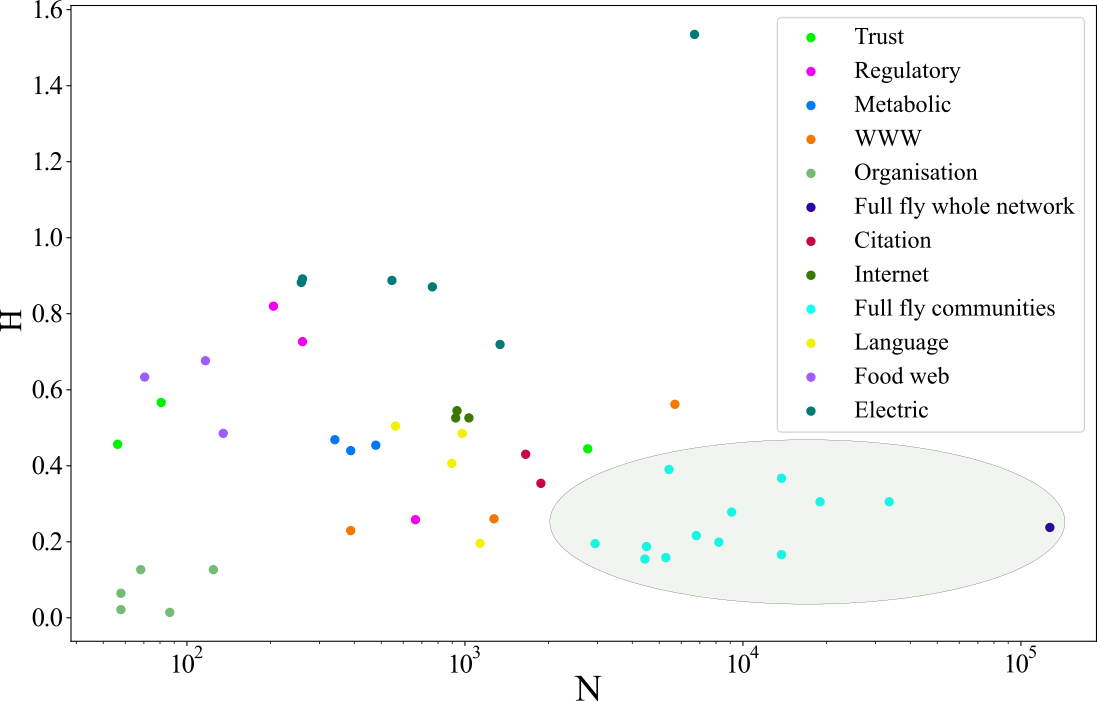
Figure 3: Here, we show the random walk hierarchy measure $H$ (Eq. (12)) of the FF connectome and all of its communities (inside the transparent ellipse) in comparison with other real world networks from [28]. Even the modules are noticeably larger than any other empirical networks considered before, they exhibit rather low level of hierarchy.

Dynamical analysis

Synchronization transition point results

In case of scenario (o) for the Kuramoto equation ($F=0$), we estimated the synchronization transition point to be at $K_{c}=0.0015(5)$, via finding an inflexion curve on the $R(t)$ growth plot (bottom inset of Fig 4), and by the fluctuation peak of $\sigma(R)$ (Fig 4). Note, that mean-field scaling is characterized by $\eta_{MF}=0.75$ [29, 24], as compared to the $\eta\simeq 1$ one can read-off from the right inset of Fig 4 at $K_{c}$, by extrapolating the local slopes to the $1/t\to 0$ limit.

Figure 4: Steady state fluctuation (standard deviation) peak of the $R$, as the function of the global coupling for the ( case o). The lower inset shows the growth of $R(t)$ for different $K$-s, while the right inset the local slopes of the growth of $R(t)$, using incoherent initial state for different $K$ global coupling values as shown by the legends. One can locate a transition at $K_{c}=0.0015(2)$, where the local slopes tend to the $\eta\simeq 1$ via a straight line approximation in the $t\to\infty$ limit.

In case of scenario (w), the transition of the Kuramoto model ($F=0$) happens at a much larger coupling: $K_{c}=1.90(2)$, estimated by the same method, displayed in Fig. 5.

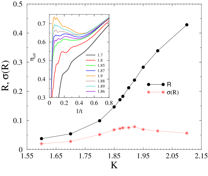
Figure 5: The Kuramoto order parameter (black bullets) and the fluctuation peak (standard deviation) of the $R$ (red stars) as the function of the global coupling for the (case w). The inset shows the local slopes of the growth of $R(t,K)$, from incoherent initial states, for different $K$ global coupling values given by the legends. This suggests a transition at $K_{c}=1.88(2)$, where the local slopes tend to $\eta=0.65(2)$, slightly below the mean-field value $\eta_{MF}=0.75$ via a straight line in the $t\to\infty$ limit. This is in agreement with the fluctuation peak value at $K_{c}\simeq 1.9$ within error margin as one can see at the bottom of the figure.

We have also investigated the $F$ and $K$ dependence of the $\sigma(R)$, i.e the SK order parameter and found that the largest fluctuation value is reached at $K_{c}\simeq 1.88$ close to the critical point without external force, as shown on Fig. 6.

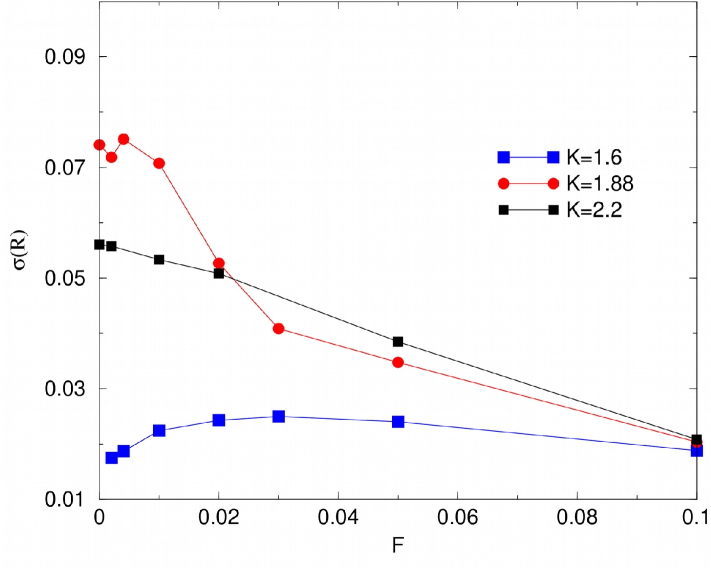
Figure 6: Dependence of the steady state SK order parameter $\sigma(R)$ on the global coupling $K$ and on the force $F$, which shows a maximum at $K_{c}$ and $F=0$.

This means maximal sensitivity of the system happens right at the critical point in the resting state. Periodic external excitations decrease the sensitivity.

Interestingly, in the case of scenario (i), we can observe two fluctuation peaks, which should be the consequence of this highly heterogeneous, directed, glassy network. By considering the inflection point of the growth we provide an estimate for the synchronization $K_{c}\simeq 0.01(5)$ as shown in Fig.7. That means we need stronger couplings to get synchronization with inhibitory links, than in case original raw graph.

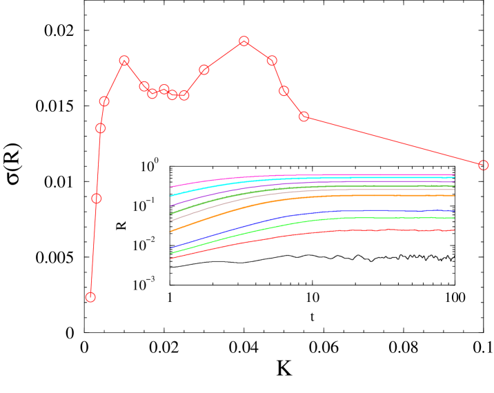
Figure 7: Steady state fluctuation peak of the $R(t\to\infty,K)$ as the function of the global coupling for the ( case i). The inset shows the growth of $R(t)$ for different $K$-s for different $K$ global coupling values: $K=$ 0.0015, 0.003, 0.004, 0.005, 0.01, 0.015, 0.02, 0.03, 0.05, 0.1 (bottom to top curves). One can observe two fluctuation peaks: $K_{c}=0.010(1)$ and $K=0.040(1)$. The temporal behavior in the inset suggests dynamical scaling (straight line) near the lower peak coupling value (orange/blue lines) at $K\simeq 0.01$.

Understanding of this anomalous behavior would require further numerical studies.

Auto-correlation results

The auto-correlation functions were found to exhibit damped oscillatory behavior after averaging over thousands of independent samples, corresponding to different self-frequencies of nodes, as shown on Fig.8. After making the absolute values of $A(t,s=1)$ we can observe an asymptotic PL decay of the tails as shown in the inset of Fig.8, which is in agreement with the critical point expectations for $y:=t/s\to\infty$.

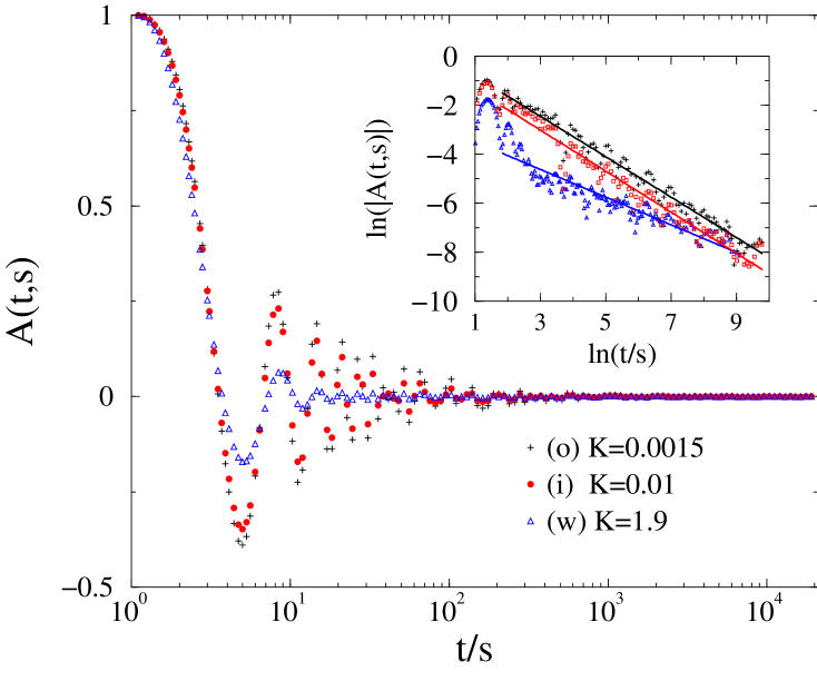
Figure 8: Critical auto-correlation functions for $s=1$ in the Kuramoto model, for different anisotropy scenarios labeled by the legends. Inset: Absolute value of the same on logarithmic scales. Dashed lines show PL fits for the tails.

The fitted tails for $\ln(y)>5$ provide the following functions: $A_{T}(t,s=1)=1.02\times t^{-0.82(2)}$ for (o); $A_{T}(t,s=1)=0.6\times t^{-0.83(2)}$ for (i), while for the weighted case (w) we obtained: $A_{T}(t,s=1)=0.05\times t^{-0.66(5)}$.

After calculating the discrete differences in $s$ as described in the Sect. Methods, we performed rescaling with $s$ and calculated the $\dot{A}(y)$ for each connectome variant, by averaging over the largest $t=258,516$ values to obtain the $y\to\infty$ asymptotic scaling. Figure 9 shows these results, as well as PL fits of the form $A_{0}+y^{A_{1}}$. We used these $\dot{A}_{T}(y)$ tail function parameters to calculate the FDR-s later in Sect. Violation of the fluctuation-dissipation.

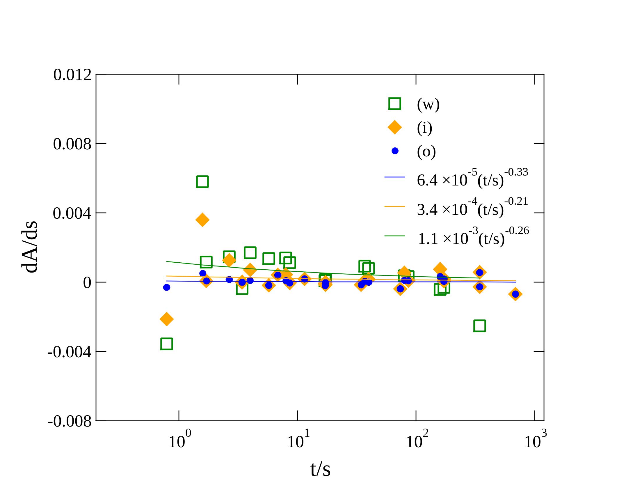
Figure 9: Summary of the $s$ derivatives of the critical auto-correlation functions: $\dot{A}(t,s)$ for scenarios (o) (bullets), (i) (rhombs) and (w) (boxes), deduced from the largest time results: $t=258$ and $516$ displayed by the legends. Lines show power law fittings assuming $A_{0}\times y^{A_{1}}$ forms for scenarios: (o), (i), (w) (top to bottom curves)

Auto-response results

We found different decays for different scenarios. This is in agreement with the spectral dimension finding that these connectomes exhibit $d_{s}<4$, thus the Kuramoto model on these connectomes does not show mean-field like scaling behavior.

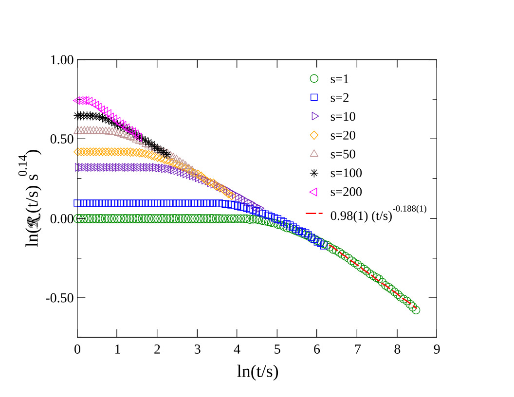
Figure 10: Scaling collapse of the auto-responses ${\cal R}(t,s)_{o}$ in the Kuramoto model for different $s$ values indicated by the legends, in case of graph scenario (o) at the estimated critical point $K_{c}=0.0015$. The dashed line shows a PL fitting for the tail: $\ln(t/s)>5$.

We applied PL fits for the tails for $\ln(y)\geq 5$ and the exponents are shown on the Figures  10 (o), 11 (i) and 12 (w). Remarkable data collapse or curves of different $s$ values could also be achieved, which provides estimates for the short-time aging exponents $1-a$, appearing to be close to $\lambda_{\cal R}/Z$ and help to deduce the asymptotic scaling behavior for $y\gg 1$.

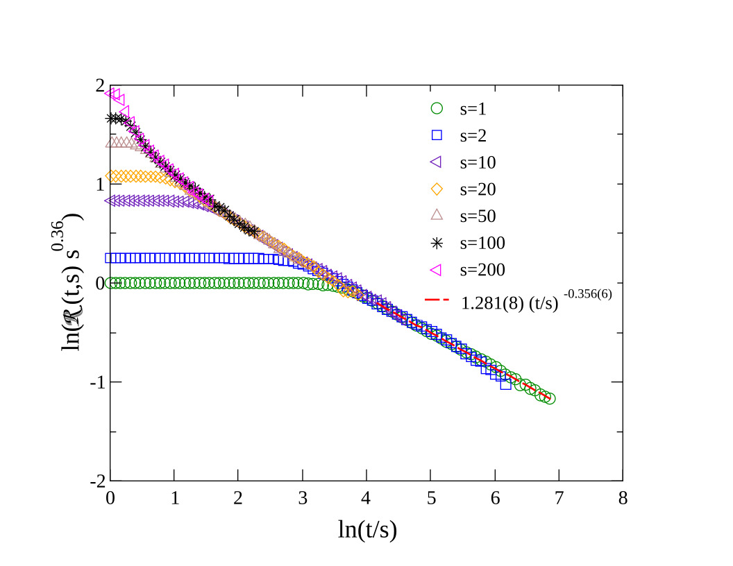
Figure 11: Scaling collapse of the auto-responses ${\cal R}(t,s)_{i}$ in the Kuramoto model for different $s$ values indicated by the legends, in case of scenario (i) at the critical point: $K_{c}=0.01$. The dashed line shows PL fitting for the tail: $\ln(t/s)>4.$

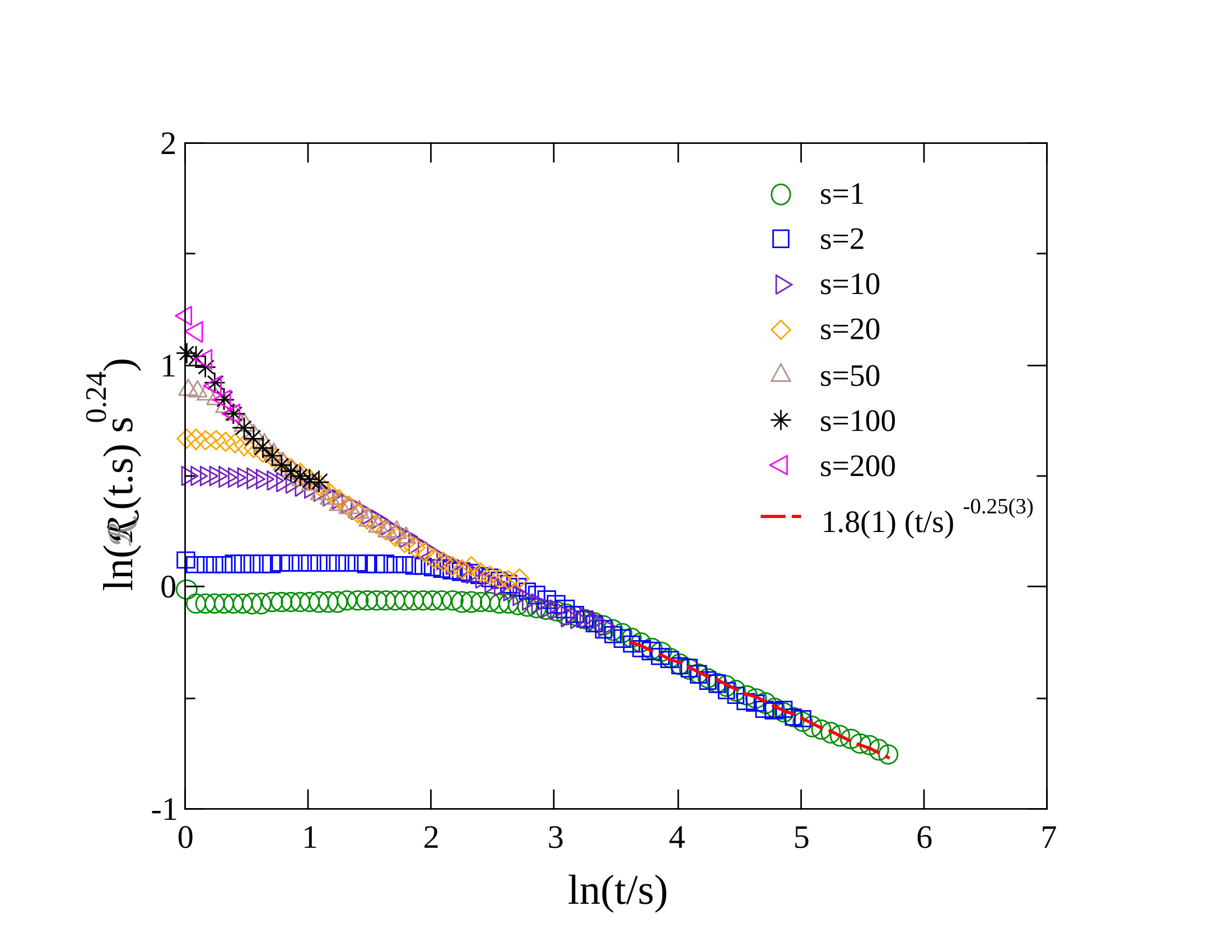
Figure 12: Scaling collapse of the auto-responses ${\cal R}(t,s)_{w}$ in the Kuramoto model for different $s$ values indicated by the legends, in case of scenario (w) at the critical point $K_{c}=1.9$. The dashed line shows PL fitting for the tail: $\ln(t/s)>4$.

Violation of the fluctuation-dissipation

Now we calculate the FDR via Eq. (6) from the numerical results of the previous subsections, using the fitted PL tail functions: $\mathrm{FDR}\simeq X(y)\simeq{R}_{T}(y)/\dot{A}_{T}(y)$ for $y=t/s\to\infty$.

For determining $X_{\infty}$ we assume that at the critical points the FDR denominators ($\dot{A}_{T}(y)$) exhibit PL behavior, similarly as the numerators: ${\cal R}(y)$ asymptotically. The following list summarizes our numerical findings, for FDR, including those for the Erdős-Rényi (ER) random graphs at the Kuramoto model criticality [30], as our reference result.

• $X(y)_{o}\simeq\displaystyle\frac{0.98(1)\times y^{-0.188(1)}}{6.4(1)\times 10^{-5}y^{-0.33(1)}}=1.5(2)10^{4}\times y^{0.14(2)}$

• $X(y)_{i}=\displaystyle\frac{1.28(1)\times y^{-0.35(1)}}{3.4(1)\times 10^{-4}y^{-0.21(1)}}=3.7(2)10^{3}\times y^{-0.14(2)}$

• $X(y)_{w}=\displaystyle\frac{1.8(1)\times y^{-0.25(3)}}{1.1(1)\times 10^{-3}y^{-0.26(1)}}=1.6(2)10^{3}y^{0.01(4)}$

• $X(y)_{ER}=\displaystyle\frac{0.21(2)\times y^{-0.32(2)}}{2.2(2)\times 10^{-5}y^{-0.30(2)}}=0.95(4)10^{4}y^{-0.02(4)}$

As we can see the FDR functions of the FF scenarios follow the expected sequence of anisotropy values: the smaller the anisotropy is, the smaller is the deviation of the FDR function from a constant within our error margins. This is seems to be true for the PL exponent magnitudes as well as for the amplitudes. Note, that at criticality $\lambda_{\mathcal{R}}=\lambda_{A}$ is expected for short-ranged and Gaussian initial correlators, which results in simple constant values for the $\lim_{y\to\infty}X(y)$ [6]. However, we did not use such initial conditions in our calculations displayed here, thus we not expect constant FDR-s even the fitted exponents are small.

For the ER model mean-field critical behavior is expected [30], but according to our knowledge no aging exponents are known [5], thus we show our numerical results for a $N=2^{17}$ sized random graph at $K_{c}\simeq 0.482$ [30] in the Supplementary Material. As this graph exhibits reciprocity of edges, we can consider it to be the most symmetric one of those we investigated here. Also ER is a graph with long-range interactions. Further study of this random graph is under way.

Unfortunately we cannot find such relation between anisotropy and FDR in the external driven case, because away from criticality both the $\dot{A}(t)$ and $\mathcal{R}(t)$ saturate to constant values and their ratio or difference is a constant, that can be related to a temperature of an equilibrium system.

Conclusions and Outlook

In conclusion we have provided numerical evidence for the relation of vFD and the network asymmetry in agreement with the expectations. The higher the link anisotropy is the larger is the FDR, thus the farher the system is from equilibrium. We determined the auto-response and auto-correlations functions at the critical state of the Kuramoto (also for SK) model on the large connectome of the fruit-fly as well as for ER graphs. As the topological dimension of the network is high first we expect close to mean-field critical behavior, however the spectral dimensions, determining the synchronization behavior on heterogeneous, non-regular graphs are found to be smaller than $d_{c}=4$, thus the temporal behavior of the these two-point functions is also non-mean-field like, they exhibit slower decay asymptotically for each anisotropy variant, than in case of the ER network. Note, however that in these strongly heterogeneous systems Griffiths effects [14] may also occur by blurring the phase transition point as in case of other complex networks [31]. The scaling collapses of the auto-response functions imply the relation: $1+a=\lambda_{\mathcal{R}/Z}$, very common in aging systems [5].

The effect of periodic force was shown to decrease the order parameter fluctuations as well as sensitivity to $F$. In terms of the global coupling control parameter $K$, our results indicate a maximal sensitivity at the critical point: $K_{c}$.

We also explored the structure of modules of the FF connectome, via community detection and the by the application of the Czégel-Palla algorithm and we found relatively low level of hierarchical organization.

As for a future work it remains to be seen the module dependence of the above results as well as exploration of the effects of forces on the aging behavior of this complex system. Our method paves the way towards the exploration of the aging behavior of oscillatory system on different regular or random graphs.

Models and Methods

The topology of the FF connectome

Community calculations

The connectome is defined as the structural network of neural connections in the brain [32]. For the "original" hemibrain connectome (HB) we used the data-set (v1.0.1) from [33]. The adjacency matrix, visualized in  [34] where one can see a rather homogeneous, almost structureless network, however it is not random [35]. The degree distribution is much wider than that of a random ER graph and exhibits a fat tail. The analysis in [34] found global weight distribution $p(w)$, with a heavy tails. Assuming a PL form, an exponent $-2.9(2)$ could be fitted for the $w>100$ region.

The modularity quotient of a network is defined by [36]

$$Q=\frac{1}{N\langle{k}\rangle}\sum\limits_{ij}\left(A_{ij}-\frac{k_{i}k_{j}}{N\langle{k}\rangle}\right)\delta(g_{i},g_{j}),$$ (7)

the maximum of this value characterizes how modular a network is, where $A_{ij}$ is the adjacency matrix, $k_{i}$, $k_{j}$ are the node degrees of $i$ and $j$ and $\delta(g_{i},g_{j})$ is $1$ when nodes $i$ and $j$ were found to be in the same community, or $0$ otherwise.

Graph dimension

We estimated the effective graph (topological) $d$ dimension, a generalization of the Euclidean dimension to graphs, by measuring shortest path chemical distances between nodes $r$ via the Breadth-first search algorithm [37]. One can give an estimate for the dimension using the definition $N(r)\sim r^{d}$, where we counted the number of nodes $N(r)$ with chemical distance $r$ or less from randomly selected seeds and calculated averages over the trials.

Spectral dimension

In case of complex networks it turned out that the so-called spectral dimension ($d_{s}$) provides a better measure for the relevancy of fluctuations in the synchronization properties [27, 38]. This is obtained from the eigenvalue spectrum of the graph Laplacian matrix and can be finite in case of complex networks, with infinite topological dimensions [39].

Graph spectral properties of complex networks have been shown to be particularly relevant to network structure [40]. Following Refs. [27, 38], we calculate the normalized Laplacian $L$ with elements

$$L_{ij}=\delta_{ij}-A_{ij}/k_{i}$$ (8)

for unweighted networks, where $k_{i}$ denotes the degree of node $i$. For weighted networks, the elements of the normalized Laplacian are given by

$$L_{ij}=\delta_{ij}-W_{ij}/k_{i}^{\prime}\,,$$ (9)

where $k_{i}^{\prime}=\sum_{j}W_{ji}$ denotes the weighted in-degree of node $i$. The normalized Laplacian has real eigenvalues $0=\lambda_{1}\leq\lambda_{2}\leq\dots\leq\lambda_{N}$, the density of which scales as [41, 27]

$$\rho(\lambda)\simeq\lambda^{d_{s}/2-1}$$ (10)

for $\lambda\ll 1$, where $d_{s}$ is the spectral dimension. The cumulative density is then given by

$$\rho_{c}(\lambda)=\int_{0}^{\lambda}d\lambda^{\prime}\rho(\lambda^{\prime})=\frac{2}{d_{s}}\lambda^{d_{s}/2}.$$ (11)

Anisotropy analysis

Additionally, we have also analyzed the graph anisotropy of communities of the FF using an algorithm by Czégel & Palla  [28], which measures the level of hierarchy via random walks and compared it with that of other well known networks as shown on Fig.3. The random walk hierarchy measure is defined as the inhomogeneity of the stationary distribution of the random walkers:

$$H=\frac{\sigma(\mathbf{p}^{stat})}{\mu(\mathbf{p}^{stat})}\ ,$$ (12)

where $\sigma$ is the standard deviation and $\mu$ is the mean, while the stationary distribution of decaying weighted random walkers is:

$$\mathbf{p}^{stat}=\frac{e^{1/\lambda}-1}{N}\sum_{n=1}^{\infty}\left(e^{-1/\lambda}\mathbf{T}\right)^{n}\mathbf{1}$$ (13)

where $T_{ij}=p(j\rightarrow i)$ is the transition matrix, $\lambda$ is the characteristic distance of a random walker. Transition of random walker: $p(j\rightarrow i)=\frac{w_{ij}}{\sum_{l}w_{lj}}\frac{w_{ij}}{\sum_{l}w_{il}}$ If update rules for $f$ random walkers are :

$$p_{i}(t)\rightarrow p_{i}(t)+\frac{f}{N};$$ (14)

$$p_{i}(t+1)=\sum_{j=1}^{N}T_{ij}p_{j}(t);$$ (15)

$$p_{i}(t+1)\rightarrow\frac{p_{i}(t+1)}{1+f}$$ (16)

Asymmetry in the interactions

As the FF original (o) structural connectome links are directed i.e. dendrites or axons, we could manipulate the level of asymmetry in the interactions without altering the topology by changing the egde weights in the following ways:

• (i) modeling inhibitions, by flipping signs of weights of $20\%$ of randomly selected edges: $W^{\prime}_{ij}=-W_{ij}$ .

• (w) modeling a local homeostasis, by renormalization of incoming link weights : $W^{\prime}_{ij}=W_{ij}/\sum_{j}W_{ij}$.

In reality both mechanism is related to the synaptic depression or inhibitions. Note, that in the FF connectome part of the nodes are glia cells, still we assume they follow the same communication structure as neurons. To quantify a measure of this anisotropy we introduced the following quantity:

$$a=1/N\sum_{i,j}^{N}(W_{ij}-W_{ji})$$ (17)

The Shinomoto-Kuramoto model with external force

We used an extended variation of the Kuramoto model of interacting oscillators [22] to study the synchronization. Oscillators with phases $\theta_{j}(t)$, $j=1,2\dots,N$ are placed on $N$ nodes of a network. They evolve according to the following set of dynamical equations

$$\dot{\theta}_{j}(t) = \omega_{j}^{0}+K\sum_{k=1}^{k=N}W_{jk}\sin[\theta_{k}(t)-\theta_{j}(t)]$$

$$+ F\sin(\theta_{j}(t))\ ,$$

where $\omega_{j}^{0}$ is the so-called self-frequency of the $j$-th oscillator, which is drawn from a Gaussian distribution, with zero mean and unit variance. The summation is performed over adjacent nodes, coupled by the $W_{jk}$ weighted adjacency matrix. In the Shinomoto extension [42] of the Kuramoto, (SK) we have a periodic force term, proportional to a coupling $F$ to describe external excitation. The global coupling $K$ is the control parameter of the model by which we can tune the system between asynchronous and synchronous states.

To locate the synchronization transition we solved the set of Eqs.The Shinomoto-Kuramoto model with external force using the Bulirsch-Stoer (BS) adaptive stepper, with step size $\delta=0.01$. The adaptive BS stepper [43, 44], which adjusts step size and degreee of function approximation to ensure a local absolute error and relative errors $\nu\leq{10^{-9}}$. We used the implementation in boost::odeint [45] with the VexCL backend [46] for support for CUDA GPUs. To find the synchronization transition we started from random initial distributions of $\theta_{j}(0)$ values, but the two-point function calculations were run from $\theta_{j}(0)\simeq 0$. In principle both initial conditions lead to the same steady state, but locating PL decay of $R(t)$ at $K_{c}$ is hard as $R(t)\to\sqrt{N}>0$ in the steady state. This is not a problem in case of measuring the two-point functions. The $t=0$ frequencies were set to be equal to the intrinsic values: $\dot{\theta}_{j}(0)=\omega_{j}^{0}$. The Kuramoto phase order parameter

$$z(t_{k})=r(t_{k})\exp\left[i\theta(t_{k})\right]=1/N\sum_{j}\exp\left[i\theta_{j}(t_{k})\right]\ .$$ (19)

was calculated at discrete time steps: $t_{k}=1+1.08^{k}$, $k=1,2,3...$ to save memory space when we are looking after the asymptotic behavior. Sample averages over different initial $\omega_{j}^{0}$ configurations were taken

$$R(t_{k})=\langle r(t_{k})\rangle$$ (20)

However, for calculating the two-point functions we had a CPU code available only, where we used the standard Runge-Kutta (RK4) solver from Numerical Recipes [47].

In the steady state, which was determined by visual inspection of the $R(t_{k},K)$ growth results from zero, we measured the standard deviations: $\sigma(R(t_{k}\to\infty,K))$ to locate $K_{c}$ as the fluctuations known to exhibit a maximum there in case of the Kuramoto model. Alternatively, half values of $R(t_{k}\to\infty,K))$ also provide an estimate for $K_{c}$.

Synchronization transition point determination

We determined the synchronization transition points of each variants: (o), (w), (i) by early time dependent runs as well as by steady state analysis. The time dependent solutions were started from fully phase disordered states and followed up to $t_{max}=300$ time steps. The sets of equations (The Shinomoto-Kuramoto model with external force) were solved numerically for $10^{3}-10^{4}$ independent initial conditions and the Kuramoto order parameter is calculated. The $R(t_{k},K)$ is non-zero above the critical coupling strength $K>K_{c}$, tends to $\propto\sqrt{1/N}$ for $K<K_{c}$, or exhibits an algebraic growth law at $K_{c}$:

$$R(t,N)=N^{-1/2}t^{\eta}f(t/N^{Z})\ ,$$ (21)

where $\eta$ is an initial growth exponent in statistical physics of non-equilibrium critical phenomena [48]. Applying a standard local slope analysis [48], defined by the logarithmic derivatives of the growth Eq. (21) at the discrete time-steps $t_{k}$, near the transition point

$$\eta_{\mathrm{eff}}=\frac{\ln R(t_{k+4})-\ln R(t_{k})}{\ln(t_{k+4})-\ln(t_{k})}\ ,$$ (22)

we estimated $K_{c}$ as well as the exponent $\eta$. Here we used the discrete time derivative step size $4$, to lessen fluctuations. In general the knowledge of the corrections to scaling allows to select a proper rescaling of the horizontal axis and one can observe a linear inflexion curve at $K_{c}$, separating the up and down veering ones, which correspond to the super and sub-critical phases. Here one can also extrapolate to the real $\eta$ exponent in the $t\to\infty$ limit. But in general, we lack the knowledge of the scaling corrections and we just try the rescaling intuitively, assuming $1/t$ usually, which corresponds to the critical behavior of simplest known non-equilibrium models.

Physical aging behavior

For analyzing the violation of FDT we measured the following difference function in Eq.(1) for the responses:

$$E_{h}(t,s)=1/N\sum_{i=1}^{N}\cos(\theta^{s}_{i}(t)-\theta_{i}(t))$$ (23)

of the angle variables $\theta_{i}(t)$ of the original and the perturbed replicas $\theta^{s}_{i}(t)$, as the response for an external small perturbation committed at the start time $s$. Similarly the real valued auto-correlations of oscillators are calculated as [49]

$$A(t,s)=1/N\sum_{i=1}^{N}\cos(\theta_{i}(t)-\theta_{i}(s)])\ .$$ (24)

In this study we applied single random perturbations at all sites : $\theta^{\prime}_{i}=\theta_{i}+h\xi_{i}$, where $\xi_{i}$ is a random variable, drawn from a zero centered Gaussian distribution and measured the auto-responses by Eq.(1) with $h=0.001$ and determined it’s start time derivatives.

Measuring two-point functions

The auto-correlator (and the response) function calculations for different $s$-values : $s=0.5,1,2,4,10,20,40,50,100,200$, were performed by a C code, which handled these functions in parallel, up to $t_{max}\leq 2000$. They were re-run for hundreds of independent initial self-frequency distributions, usually starting from phase synchronized states, and averaged over finally. We also performed tests by starting from random phase distributions, but in that case the fluctuation effects were stronger.

From these extensive calculations we determined the $s$ derivatives of the correlators: $dA(t,s)/ds:=\dot{A}(t,s)$. For simplicity we reduced the two-point functions to be variables of $t/s=y$, which is expected to be the main variable in aging system at criticality [5], providing the autocorrelation and auto-response exponents in the $y\to\infty$ limit, as shown in Eq. 3.

Supplementary Material

Here we show our aging and FDR results for random ER graphs with average degree $\langle k\rangle=4$. Most calculations were done for $N=2^{17}$ at $K=0.482$, which was obtained for the Kuramoto model in such networks [30]. We tried this both for the phase ordered and disordered initial conditions, but for the ordered (phase-correlated, frequency uncorrelated) case the ${\cal R}(y)$ seems go to a non-zero saturation value for $y\to\infty$ as some recent works found for the auto-correlator, in case of quenches to the ordered phase [50]. Assuming such saturation value (${\cal R}(y\to\infty)=0.02$), we have a rough estimate: $\lambda_{\cal R}/Z=\lambda_{A}/Z\simeq 0.65(5)$ for for this initial condition. Furthermore, the $\dot{A}(y)$ function seems to grow with $y$, unlike for the other cases considered here, which provides a very uncertain estimate for the FDR. Further investigation of this is under way and will be published somewhere else.

In the case of random (fully uncorrelated) phases and self-frequencies we obtained a reasonable scaling within the computing possibilities as shown in Figs.. 13 and 14.

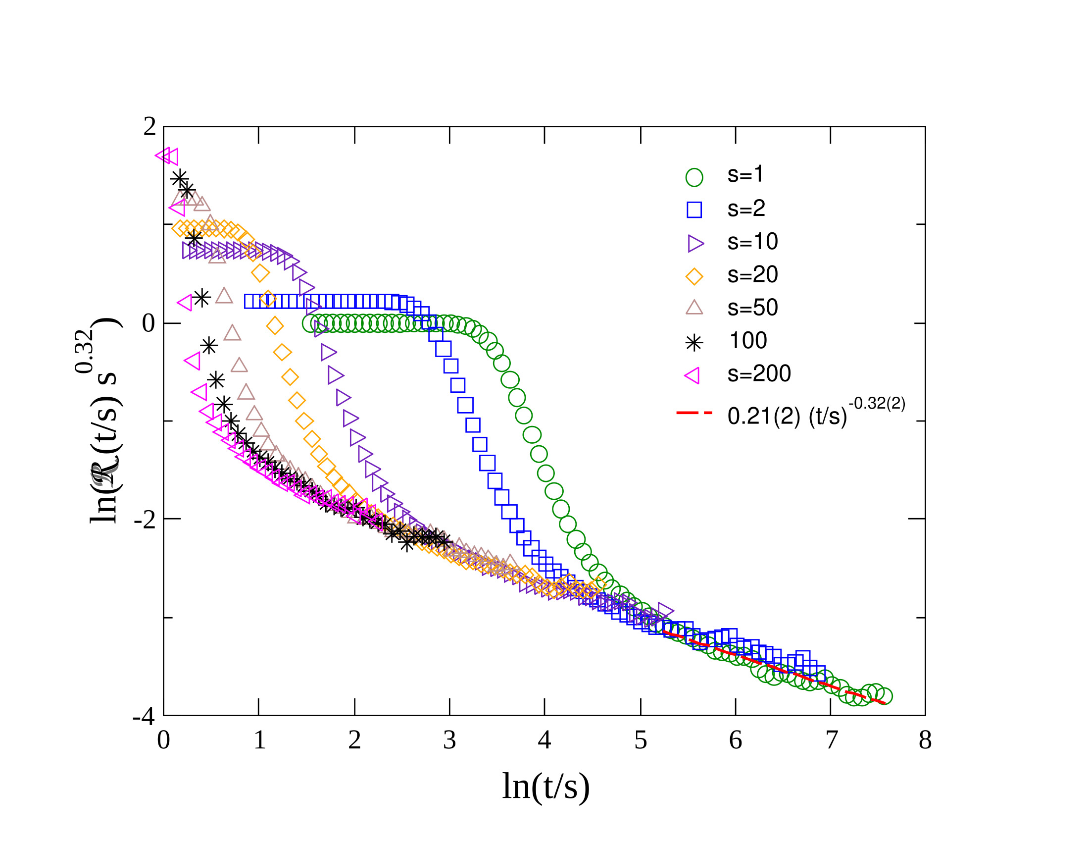
Figure 13: Scaling collapse of the auto-responses in the Kuramoto model for $s$ values indicated by the legends, in case of the ER graph at the critical point $K_{c}\simeq 0.482$. The dashed line shows a PL fitting for the tail: $\ln(t/s)>5$, with an exponent: $\lambda_{R}/Z=0.32(2)$

Here averaging was performed for $\simeq 600$ realizations up to $t_{max}=2000$.

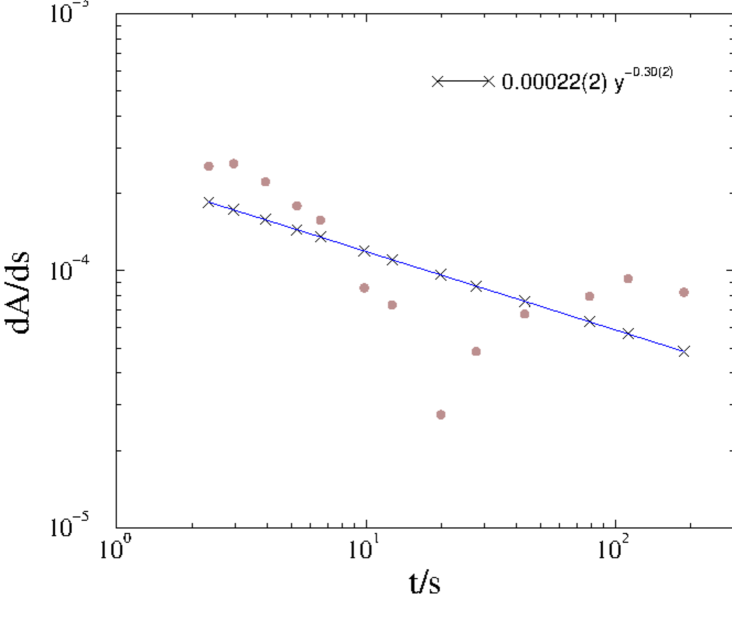
Figure 14: Here we see the $s$ derivatives of the auto-correlations: $\dot{A}(t,s)$ of the critical Kuramoto on ER graph in case of phase disordered initial state, deduced from the results of $t=120$ and $258$ as shown by the bullets. The line shows a power law fitting assuming with a PL exponent $-0.30(2)$

As the fitted tail exponents of $R(y)$ and $\dot{A}(y)$ are very close in the FDR ratio, they almost cancel out, suggesting closeness to the equilibrium in case of this reciprocal and symmetric graph with the Kuramoto dynamics.

References

- [1] Cugliandolo, L. F., Dean, D. S. & Kurchan, J. Fluctuation-dissipation theorems and entropy production in relaxational systems. \JournalTitlePhys. Rev. Lett. 79, 2168–2171, DOI: 10.1103/PhysRevLett.79.2168 (1997).
- [2] Marconi, U. M. B., Puglisi, A., Rondoni, L. & Vulpiani, A. Fluctuation–dissipation: Response theory in statistical physics. \JournalTitlePhysics Reports 461, 111–195, DOI: https://doi.org/10.1016/j.physrep.2008.02.002 (2008).
- [3] Deco, G., Lynn, C. W., Sanz Perl, Y. & Kringelbach, M. L. Violations of the fluctuation-dissipation theorem reveal distinct nonequilibrium dynamics of brain states. \JournalTitlePhys. Rev. E 108, 064410, DOI: 10.1103/PhysRevE.108.064410 (2023).
- [4] Monti, J. M., Perl, Y. S., Tagliazucchi, E., Kringelbach, M. L. & Deco, G. Fluctuation-dissipation theorem and the discovery of distinctive off-equilibrium signatures of brain states. \JournalTitlePhys. Rev. Res. 7, 013301, DOI: 10.1103/PhysRevResearch.7.013301 (2025).
- [5] Henkel, M. & Pleimling, M. Non-Equilibrium Phase Transitions: Volume 2: Ageing and Dynamical Scaling Far from Equilibrium. Theoretical and Mathematical Physics (Springer Netherlands, 2011).
- [6] Henkel, M. Generalised time-translation-invariance in simple ageing. In Dobrev, V. (ed.) Lie Theory and Its Applications in Physics, 93–109 (Springer Nature Singapore, Singapore, 2025).
- [7] Cocchi, L., Gollo, L. L., Zalesky, A. & Breakspear, M. Criticality in the brain: A synthesis of neurobiology, models and cognition. \JournalTitleProgress in Neurobiology 158, 132–152, DOI: https://doi.org/10.1016/j.pneurobio.2017.07.002 (2017).
- [8] Muñoz, M. A. Colloquium: Criticality and dynamical scaling in living systems. \JournalTitleRev. Mod. Phys. 90, 031001, DOI: 10.1103/RevModPhys.90.031001 (2018).
- [9] Ódor, G., Gastner, M. T., Kelling, J. & Deco, G. Modelling on the very large-scale connectome. \JournalTitleJournal of Physics: Complexity 2, 045002, DOI: 10.1088/2632-072x/ac266c (2021).
- [10] Kinouchi, O. & Copelli, M. Optimal dynamical range of excitable networks at criticality. \JournalTitleNature Physics 2, 348–352, DOI: 10.1038/nphys289 (2006).
- [11] Chialvo, D. R. Emergent complex neural dynamics. \JournalTitleNature Physics 6, 744–750 (2010).
- [12] Larremore, D. B., Shew, W. L. & Restrepo, J. G. Predicting criticality and dynamic range in complex networks: Effects of topology. \JournalTitlePhys. Rev. Lett. 106, 058101, DOI: 10.1103/PhysRevLett.106.058101 (2011).
- [13] Bak, P., Tang, C. & Wiesenfeld, K. Self-organized criticality: An explanation of the 1/f noise. \JournalTitlePhys. Rev. Lett. 59, 381–384, DOI: 10.1103/PhysRevLett.59.381 (1987).
- [14] Griffiths, R. B. Nonanalytic Behavior Above the Critical Point in a Random Ising Ferromagnet. \JournalTitlePhys. Rev. Lett. 23, 17–19, DOI: 10.1103/PhysRevLett.23.17 (1969).
- [15] Muñoz, M. A., Juhász, R., Castellano, C. & Ódor, G. Griffiths Phases on Complex Networks. \JournalTitlePhys. Rev. Lett. 105, 128701 (2010).
- [16] Moretti, P. & Muñoz, M. A. Griffiths phases and the stretching of criticality in brain networks. \JournalTitleNature Communications 4, 2521, DOI: 10.1038/ncomms3521 (2013).
- [17] Ódor, G., Dickman, R. & Ódor, G. Griffiths phases and localization in hierarchical modular networks. \JournalTitleScientific Reports 5, 14451 (2015).
- [18] Ódor, G. Critical dynamics on a large human open connectome network. \JournalTitlePhysical Review E 94, 062411 (2016).
- [19] Blondel, V. D., Guillaume, J.-L., Lambiotte, R. & Lefebvre, E. Fast unfolding of communities in large networks. \JournalTitleJournal of Statistical Mechanics: Theory and Experiment 2008, P10008 (2008).
- [20] Flywire connectome data (2023).
- [21] Cirunay, M., Ódor, G. & Papp, I. Scale-free behavior of weight distributions of connectomes (2024). 2407.17220.
- [22] Kuramoto, Y. Chemical Oscillations, Waves, and Turbulence. Springer Series in Synergetics (Springer Berlin Heidelberg, 2012).
- [23] Hong, H., Park, H. & Choi, M. Collective synchronization in spatially extended systems of coupled oscillators with random frequencies. \JournalTitlePhysical Review E - Statistical, Nonlinear, and Soft Matter Physics 72, DOI: 10.1103/PhysRevE.72.036217 (2005).
- [24] Ódor, G., Deng, S. & Kelling, J. Frustrated synchronization of the kuramoto model on complex networks. \JournalTitleEntropy 26, DOI: 10.3390/e26121074 (2024).
- [25] Abrams, D. M. & Strogatz, S. H. Chimera states for coupled oscillators. \JournalTitlePhys. Rev. Lett. 93, 174102, DOI: 10.1103/PhysRevLett.93.174102 (2004).
- [26] Wu, K. & Simon, H. Thick-restart lanczos method for large symmetric eigenvalue problems. \JournalTitleSIAM Journal on Matrix Analysis and Applications 22, 602–616, DOI: 10.1137/S0895479898334605 (2000). https://doi.org/10.1137/S0895479898334605.
- [27] Millán, A. P., Torres, J. J. & Bianconi, G. Complex network geometry and frustrated synchronization. \JournalTitleScientific reports 8, 1–10 (2018).
- [28] Czégel, D. & Palla, G. Random walk hierarchy measure: What is more hierarchical, a chain, a tree or a star? \JournalTitleScientific Reports 5, 17994, DOI: 10.1038/srep17994 (2015).
- [29] Choi, C., Ha, M. & Kahng, B. Extended finite-size scaling of synchronized coupled oscillators. \JournalTitlePhysical Review E - Statistical, Nonlinear, and Soft Matter Physics 88, DOI: 10.1103/PhysRevE.88.032126 (2013).
- [30] Juhász, R., Kelling, J. & Ódor, G. Critical dynamics of the Kuramoto model on sparse random networks. \JournalTitleJournal of Statistical Mechanics: Theory and Experiment 2019, 053403, DOI: 10.1088/1742-5468/ab16c3 (2019).
- [31] Attwell, D. & Laughlin, S. B. An energy budget for signaling in the grey matter of the brain. \JournalTitleJournal of Cerebral Blood Flow & Metabolism 21, 1133–1145, DOI: 10.1097/00004647-200110000-00001 (2001). PMID: 11598490.
- [32] Sporns, O., Tononi, G. & Kötter, R. The Human Connectome: A Structural Description of the Human Brain. \JournalTitlePLOS Computational Biology 1, e42, DOI: 10.1371/journal.pcbi.0010042 (2005).
- [33] The hemibrain dataset (v1.0.1) (2020).
- [34] Ódor, G., Deco, G. & Kelling, J. Differences in the critical dynamics underlying the human and fruit-fly connectome. \JournalTitlePhys. Rev. Research 4, 023057, DOI: 10.1103/PhysRevResearch.4.023057 (2022).
- [35] Scheffer, L. K. Graph properties of the adult drosophila central brain, DOI: 10.1101/2020.05.18.102061 (2020).
- [36] Newman, M. E. J. Modularity and community structure in networks. \JournalTitleProc Natl Acad Sci U S A 103, 8577–8582 (2006).
- [37] Lee, C. Y. An algorithm for path connections and its applications. \JournalTitleIRE Transactions on Electronic Computers EC-10, 346–365, DOI: 10.1109/TEC.1961.5219222 (1961).
- [38] Millán, A. P., Torres, J. J. & Bianconi, G. Synchronization in network geometries with finite spectral dimension. \JournalTitlePhysical Review E 99, 022307 (2019).
- [39] Poggialini, A., Villegas, P., Muñoz, M. A. & Gabrielli, A. Networks with many structural scales: A renormalization group perspective. \JournalTitlePhys. Rev. Lett. 134, 057401, DOI: 10.1103/PhysRevLett.134.057401 (2025).
- [40] Chung, F. R. Spectral graph theory, vol. 92 (American Mathematical Soc., 1997).
- [41] Burioni, R. & Cassi, D. Universal properties of spectral dimension. \JournalTitlePhysical review letters 76, 1091 (1996).
- [42] Shinomoto, S. & Kuramoto, Y. Phase Transitions in Active Rotator Systems. \JournalTitleProgress of Theoretical Physics 75, 1105–1110, DOI: 10.1143/PTP.75.1105 (1986).
- [43] Bulirsch, R. & Stoer, J. Numerical treatment of ordinary differential equations by extrapolation methods. \JournalTitleNumerische Mathematik 8, 1–13 (1966).
- [44] P., D. Order and stepsize control in extrapolation methods. \JournalTitleNumerische Mathematik 41, 399–422 (1983).
- [45] Ahnert, K. & Mulansky, M. Boost::odeint.
- [46] Demidov, D. Vexcl.
- [47] Press, W., Teukolsky, S., Vetterling, W. & Flannery, B. Numerical Recipes 3rd Edition: The Art of Scientific Computing (Cambridge University Press, 2007).
- [48] Ódor, G. Universality in nonequilibrium lattice systems: Theoretical foundations (World Scientific, 2008).
- [49] Acebrón, J., Bonilla, L., Vicente, C., Ritort, F. & Spigler, R. The kuramoto model: A simple paradigm for synchronization phenomena. \JournalTitleReviews of Modern Physics 77, 137–185, DOI: 10.1103/RevModPhys.77.137 (2005).
- [50] Christiansen, H., Majumder, S., Janke, W. & Henkel, M. Finite-size effects in aging can be interpreted as sub-aging (2025). 2501.04843.