Scale-free behavior of weight distributions of connectomes

Abstract

To determine the precise link between form and function, brain studies primarily concentrate on the anatomical wiring of the brain and its topological properties. In this work, we investigate the weighted degree and connection length distributions of the KKI-113 and KKI-18 human connectomes, the fruit fly, and of the mouse retina. We found that the node strength (weighted degree) distribution behavior differs depending on the considered scale. On the global scale, the distributions are found to follow a power-law behavior, with a roughly universal exponent close to 3. However, this behavior breaks at the local scale as the node strength distributions of the KKI-18 follow a stretched exponential, and the fly and mouse retina follow the log-normal distribution, respectively which are indicative of underlying random multiplicative processes and underpins non-locality of learning in a brain close to the critical state. However, for the case of the KKI-113 and the H01 human (1mm³) datasets, the local weighted degree distributions follow an exponentially truncated power-law, which may hint at the fact that the critical learning mechanism may have manifested at the node level too.

1 Introduction

In neuroscience, networks-based analysis is heavily needed as the brain is a complex system made up of many interacting neurons [1]. Understanding the structure of these connections is crucial as form is believed to be highly linked with function [2]. The objective description of the nodes’ and edges’ contributions to the network as a whole is made possible by the network metrics. Regardless of how widely dispersed or how closely spaced apart they are, nodes with similar qualities can be grouped into a single structurally defined class [3].

In literature, one may find many attempts to investigate how the morphological and topological quantities related to neuronal development. For example, earlier works on the structural neural circuits of the cerebral cortex characterized the cortex as a mixing device whose corticocortical connections are primarily determined by chance and may be further refined during the learning process [4]. An even older model of neural networks, which Beurle thought might be shaped by learning and plasticity, was based on random connectivity, an unstructured substrate, in parallel with these neuroanatomical concepts [5]. Recently models were proposed, in which network optimization is taken into account, for example, Lynn et a [6] proposed a model in which following a random edge pruning new link is added either by a preferential attachment or randomly. This provides heavy-tailed connection strengths in agreement with the connectomes they considered.

Others have even looked at combined topological and spatial properties of neural networks by making an analogous physical construct of connectomes, which they called contactomes [7], and found that optimization with certain boundary conditions leads to degree and distance distributions close to the neural connectomes in the fruit fly, mouse, and human and unveil a simple set of shared organizing principles across these organisms.

While neuronal distance distributions are known to follow exponential rule [8], degree distributions exhibit more fat-tailed like distribution tails, typically stretched exponential [9]. Scale-free behavior was found at the global level of weights in case of large human white matter boundles [10] and in case of neural links of the hemibrain [11].

It was previously hypothesized that functional brain networks follow scale-free behaviors characterized by the presence of power-laws [12, 13]. Power-laws signal a certain amount of self-organization, either through replication (as in biological/metabolic networks) or growth and preferential attachment (as in sociological/technological networks) [14, 15]. Moreover, it has been proposed that the so-called scale-free property enables effective communication using a limited number of core nodes that serve as information flow hubs such as in the case of transportation or airline networks [16]. In statistical physics, power laws are important because they appear when there is a change from an ordered to an unordered phase in the absence of a distinctive length scale. The brain functions close to this crucial region, according to theoretical and empirical evidence [17, 18, 19, 20, 21].

In this work, we investigate how critical learning mechanisms affect the weight and strength distributions of node connections of human and non-human connectomes on both the global and the local scale. To serve as a developmental comparison, we compare a fruit fly larva to that of an adult fruit fly brain.

2 Methodology

The connectome is defined as the structural network of neural connections in the brain [22]. At the size of a single neuron, existing imaging methods are unable to fully resolve the roughly $\approx 10^{11}$ neurons that make up the human brain. In this work, we employed coarse-grained networks, acquired using diffusion tensor imaging, including $\approx 10^{6}$ nodes which is found to agree well with ground-truth data from histology tract tracing [23, 24]. Such large, whole-brain network data are obtained from the Open Connectome Project repository and have been previously analyzed [9]. Here, we consider three connectome datasets: KKI-113, KKI-18, fruit fly, and the mouse retina. Table 1 shows the network properties of these datasets.

Table 1: Properties of the Giant Connected Components (GCC) of the networks considered

Dataset	No. of Nodes	No. of Edges
KKI-113	799,133	48,096,501
KKI-18	797,759	46,524,003
H01 Human (1mm3)	13,579	76,004
Mouse retina	1,076	577,350
Fly (Hemibrain)	21,662	3,413,160
Fly (Hemibrain reciprocated)	16,804	3,251,362
Fly (Full brain)	124,778	3,794,527
Fly (Larva)	2,952	110,677

The KKI-113 network contains $799,113$ nodes and $48,096,500$ weighted and directed edges. On the other hand, the KKI-18 contains $836,733$ nodes and $46,524,003$ weighted and directed connections [25, 26]. Additionally, the human H01 (1mm³) dataset which contains $13,579$ nodes and $76,004$ edges [7]. The enormous number of nodes results from the usage of various parcellations that are closer to voxel resolution. For instance, the brain masks of a conventional aligned MRI with 1mm resolution include about 1.8 million voxels. Finally, to serve as a comparison, we also consider a fly’s full brain with $124,778$ nodes and $3,794,527$ edges; [27] a fly hemibrain [28] (with $21,662$ nodes and $3,413,160$ edges) connectomes and its bidirectional version (with $16,804$ nodes and $3,251,362$ reciprocal edges). Additionally, to investigate the changes in a fly’s brain, we included a fly larva dataset [29] with $2,952$ nodes and $110,677$ edges. Finally, we also include the mouse retina data set, with only $10,76$ nodes and $577,350$ weighted and directed edges [30].

The global node strength $w_{i}$ refers to the number of edges that surround a particular node $i$. In weighted networks, the node strength is the generalization of the node degree, or how strongly a node is connected to the rest of the nodes in the networks [31]. Additionally, we also present results on the distribution of the voxel Euclidean distances of the largest human connectome, the KKI-113 in addition to the previously reported topological properties for other human connectomes [9]. We take particular interest in the global and local weight distributions of these connectomes.

The weighted node out-degree/strength $s_{i}^{out}$ is the sum of the edge weights for outgoing edges incident to that node [31]. Here, the weights $w_{ji}$ (or $w_{ij}$) correspond to the number of connecting fibers between two nodes in the network.

$$s_{i}^{out}=\sum_{j}a_{ij}w_{ij}$$ (1)

Similarly, the weighted in-degree/strength $s_{i}^{in}$ is the sum of the incoming edge weights for links incident to that node.

$$s_{i}^{in}=\sum_{j}a_{ji}w_{ji}$$ (2)

3 Results

3.1 Human white matter

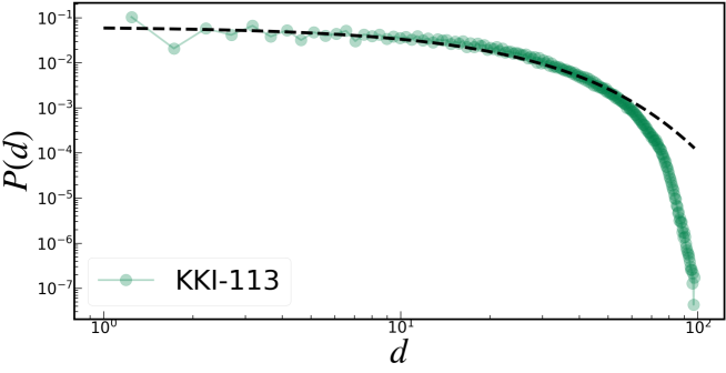
Figure 1: The neuronal distance of KKI-113 is found to follow an exponential decay with a distance scale of $d_{0}=15.71$ mm.

To describe the spatial arrangement of KKI-113, we regard nodes, whose location coordinates $(x,y,z)$ correspond to its center. Here, we computed the Euclidean distance between them and obtained the distribution displayed in Figure 1. In literature, neuronal distances are known to follow the exponential rule $p(d)\propto e^{-d/d_{0}}$  [8]. Previous works have hypothesized that the establishment and maintenance of synapses in neural connectomes is connected to wiring cost, which aligns with the concept of exponential decay [32, 33, 34]. By visual inspection, the distribution of the neuronal distances for KKI-113 seems to agree with such a concept with a characteristic value of $d_{0}=15.71$ mm corresponding to the mean of the data. As one may observe the tail is found to decay faster. This may be due to the limitations of the Diffusion Tensor Imaging which was employed for data acquisition wherein there is a possibility of underestimating long-distance connections [35, 36] and overestimating local connections [37] as in the case of the typical global tractography approach in which streamlines weighted with their corresponding fiber lengths are traced to connect pairs of given voxels [38]. Although more recent work on the use of diffusion MRI tractography and histological tract-tracing applied on ferret brain have shown good agreement between anatomical experiments and the estimates done for the case of mouse and monkey [24] increasing confidence in the technique, we believe that the observed faster decay for the case of KKI-113 was due to this imaging limitation and the fact that the human brain is far more complex and contains more white matter than any other nonhuman primates [39], which may have caused the difficulty in delineating neuronal connections, especially at large distances. Moreover, it has been suggested that in larger brains, long-range connections may require greater axon diameters in order to sustain fast neural transmission [40, 41] and that certain types of high-cost connectivity may be less common in larger brains [42].

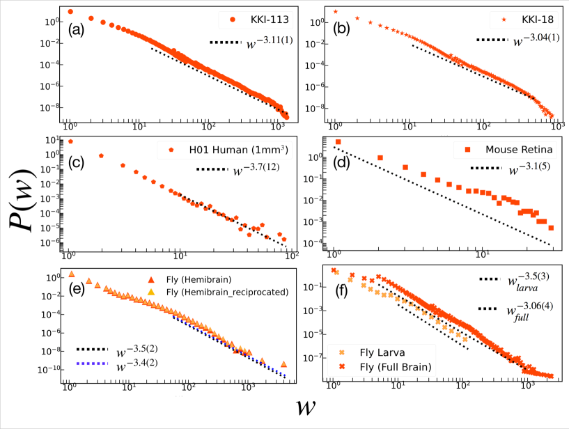
Figure 2: The weight distributions of (a) KKI-113 (b) KKI-18 (c) H01 Human (1mm³) (d) Mouse Retina (e)Fly (Hemibrain) (f) Fly (Full Brain) and that of a larva’s all follow power-law behaviors in the global scale.

Table 2: Global weight distributions fitting parameters

Dataset	PL exponent, $\alpha$	KS Distance, $D$
KKI-113	3.11(1)	0.040
KKI-18	3.04(1)	0.052
H01 Human (1mm3)	3.7(12)	0.057
Mouse Retina	3.1(5)	0.087
Fly (Hemibrain) [FHB]	3.5(2)	0.013
Fly (Hemibrain reciprocated) [FHBR]	3.4(2)	0.019
Fly (Full Brain) [FFB]	3.06(4)	0.030
Fly (Larva) [FL]	3.5(3)	0.070

Although individual neurons in the brain can only carry out relatively simple computations on their own, cell networks in the brain can undertake sophisticated operations that result in adaptive behaviors. In critical dynamics, scale-invariant metrics can be used to characterize the scale-invariant structure. The power laws observed in the system’s characteristic distribution have been identified as common indicators of criticality among various metrics. Criticality has been hypothesized to govern the dynamics of nervous system activity because of its many properties that maximize information processing. Power-law distribution analysis is a tool used to look into the criticality of nervous system data [43].

Figure 2 shows the global weight distributions of the KKI-113, KKI-18, human H01 (1mm³), mouse retina, and the hemi- and full brain of fruit flies, and that of a fruit fly larva. We employed the statistical framework of Clauset et.al. [44] to identify and measure power-law behavior. While there are contentions on the accuracy of the method in detecting power-laws, which can be affected by factors like the range of data being fitted, we have checked the goodness-of-fit by computing the Kolmogorov-Smirnov (K-S) distance $D$ and the standard error coefficient $\sigma$. The exponent which minimizes this value is displayed on the Figure. As previously noted, scale-free behavior may be generated via self-organization or via preferential attachment growth [14, 15] which allows for effective communication using a limited number of core nodes that serve as information hubs [16].

Note that the global weight distribution of the KKI-18 (Figure 2(b)) has been previously investigated [10], with a power-law fit of $\alpha=3.05(5)$. This was obtained for data with a size of $N=41,523,931$. This time, however, we obtained a more complete graph with $N=46,524,003$, such that the power-law exponent varied slightly with an exponent of $\alpha=3.04(1)$. In Figure 2(e)-(f), we can observe that the power-law exponents pertaining to that of the fruit fly data sets, $\alpha_{full}<\alpha_{hemi}<\alpha_{larva}$, where the larva has the largest exponent value (steepest), which meant high probability of finding nodes that have fewer links or weaker connections to its neighbors which is consistent with the fact that at this stage, the fruit fly is still in its formative stages of development. Moreover, this state of the larva network where there is a lack of large values of edge weights, may be thought of as its ”pre-learning” phase, where neuroplasticity has not occurred yet. Finally, the opposite can be observed for the full brain of an adult fruit fly which has the lowest value of power-law exponent. This means a lower probability of low-value weights and more likelihood of finding high-edge weights as indicated by its fat tail. The presence of high-edge weights may be an indication of the structural and functional reinforcements that have occurred throughout the phases of a fly’s development.

Figure 3: Local weighted degree (node strength) distributions do not follow a power-law behavior anymore. The weighted local in/out-degree of the KKI-113 are shown to behave as an exponentially truncated power-law (shown in (a)-(c)). Meanwhile, KKI-18 follows a stretched exponential ((d)-(f)). The human H01 (1mm³) distributions ((g)-(i)), on the other hand, follow an exponentially truncated power-law. Finally, the weighted degree distributions of the mouse retina ((j)-(l)), and the hemi- ((m)-(o)), full brain ((p)-(r)) of a fruit fly and that of a larva having considerably smaller spatial sizes, all follow log-normal distributions.

Table 3: Local strength distributions fitting parameters

Dataset Fitting Function Parameters $s_{in}$ $s_{out}$ $s_{total}=s_{in}+s_{out}$ KKI-113 Exp. Truncated PL $C=1.17$ $s_{o}=0.189$ $\beta=0.150$ $\kappa=1371$ $C=1.17$ $s_{o}=0.189$ $\beta=0.150$ $\kappa=1378$ $C=1.17$ $s_{o}=0.189$ $\beta=0.147$ $\kappa=1682$ KKI-18 Stretched Exp. $A_{o}=104.12$ $\gamma=0.44$ $A_{o}=89.03$ $\gamma=0.41$ $A_{o}=209.48$, $c=0.45$ H01 Human (1mm³) Exp. Truncated PL $C=1.20$ $s_{o}=1.17$ $\beta=0.281$ $\kappa=40.9$ $C=1.20$ $s_{o}=1.17$ $\beta=0.281$ $\kappa=41.3$ $C=1.20$ $s_{o}=-0.031$ $\beta=0.203$ $\kappa=61.2$ Mouse Retina Lognormal $\mu=5.96$, $\sigma=0.81$ $\mu=5.77$, $\sigma=1.09$ $\mu=6.62$, $\sigma=0.85$ Fly (Hemibrain) [FHB] Lognormal $\mu=4.75$, $\sigma=0.79$ $\mu=4.71$, $\sigma=0.84$ $\mu=5.45$, $\sigma=0.78$ Fly (Hemibrain reciprocated) [FHBR] Lognormal $\mu=4.97$, $\sigma=0.77$ $\mu=4.94$, $\sigma=0.80$ $\mu=5.70$, $\sigma=0.72$ Fly (Full Brain) [FFB] Lognormal $\mu=2.22$, $\sigma=1.59$ $\mu=2.36$, $\sigma=1.50$ $\mu=3.02$, $\sigma=1.48$ Fly (Larva) [FL] Lognormal $\mu=3.41$, $\sigma=0.68$ $\mu=3.43$, $\sigma=0.65$ $\mu=4.12$, $\sigma=0.63$

Figure 3 shows the local in-, out-, and total (in+out) node strength distributions for all datasets considered. For the case of KKI-113 (shown in Figure 3(a)-(c)) and the human H01 (1mm³) datasets, the strength distributions are found to follow an exponentially truncated power-law, also consistent with other large human connectomes [9]. We believe that this is in accordance with the critical learning mechanisms that have been observed at the global weight distributions (see Figure 2) and can manifest on the node-level too. The truncation may be due to some physical constraints. For example, Mossa et. al. attributed the truncation on the degree distributions of the World Wide Web (WWW) and the University of Notre Dame domain, to the limitation in information-processing capabilities of the nodes. As there is a cost associated with information-processing, there was a need to filter incoming information based on interest. By doing so, the new nodes in the network only process a subset of the information from existing nodes [45]. As the brain itself is an information-processing unit, we believe that this may also explain the truncation in the local weighted degree distributions of the KKI-113 and the H01 (1mm³) datasets, wherein neuronal connections and exchanges only occur with a subset of local neighbors. Additionally, in systems that restrict the maximum number of linkages a node can have, such as the local neighborhood being considered, the scale-free characteristic is not to be expected. The ability of the nodes to link to an arbitrary number of other nodes is necessary for the scale-free property to appear.

Stretched exponential and lognormal distributions may arise from multiplicative processes. In fact, in some cases, Laherre and Sornette proposed the stretched exponential as an alternative to the power-law [46]. With multiplicative phenomena, one instance can multiply rapidly, triggering a cascade. When something is of this nature, individual instances are not independent of one another. These behaviors can be expected to arise from a high level of connectivity. Here, we observe that such distributions not only describe the possible types of events or cascade that flow through these connections i.e. electrical signal, infection, etc., but this time, they describe the level of connectivity itself (i.e. weighted degree). As shown in Figure 3, local node strengths ($s_{in}$, $s_{out}$, and $s_{tot}$) of the KKI-18 [(d)-(f)], the mouse retina [(j)-(l)] and the fruit fly [(m)-(r)], are found to follow the stretched exponential or log-normal distributions, respectively. The former is consistent with a previous work on other large human connectomes [9]. We surmise that this multiplicative creation of connections has resulted from neuroplasticity or the brain’s ability to reorganize functionally and structurally as a response to external stimuli [47, 48, 49]. Such connections are the physical reinforcements that were created during the different stages of development of the human and mouse.

The formation of synapses in the brain is thought to have begun with mostly undirected ”exploratory” extension, which is followed by selective consolidation and contact dissolution in an early developmental model. The first process might be termed random, whereas the second process transmits specificity since it is primarily driven by neural activity or biochemical interactions between participating cells [50]. As the brain connections were first thought to be random and later shaped by learning and plasticity [4, 5], this may explain the observed lognormal behaviors that hint at the underlying random multiplicative processes that have occurred in the system.

It may appear difficult for spatially embedded networks to exhibit scale-free behavior because of the inherent limitations imposed by basic spatial and metabolic constraints [3] on the density and number of connections that may be maintained at any given node. An exponential and exponentially truncated power-law was seen in different spatial networks, including transportation networks [51, 52], which we have also observed as in the case of the human connectomes, KKI-113, KKI-18, and H01 (1mm³) as shown in Figure 3(a)-(i). However, for even more constrained brain networks such as the case of the mouse and fly, we may not observe distributions of connections that are near to scale-free.

The distributions of the mouse and that of the fly (hemi, larva, and full brain) follow the lognormal trend which deviates a little bit from the normal Gaussian and exponential due to occurrences of large connections but whose tails are not as fat as a power-law’s. We may then consider these networks to have connection strengths that are homogeneous single-scale and not scale-free [3] as indicated by their well-defined mean and standard deviation (and consequently variance). Notice, however, that for the datasets following log-normal behaviors, the parameters $\mu$ and $\sigma$ (the mean and standard deviation of the natural logarithm of the strengths) for the in and out strength distributions are close in value which may hint at the degree of symmetry or reciprocity of the connections at the local scale. This so-called reciprocity of pathways and connectivity has also been observed in the macaque visual cortex [53] and mammalian cortex [54]. This is also shown in case of the Full-fly, see [55] This may be a manifestation of specificity in the form of link consolidation [50]. Expectantly, the values of such parameters for the total (in + out) strength distributions will be slightly larger.

Table 4: Summary of source and sink nodes

Dataset No. source nodes Max. $s_{out}$ $\left<s_{out}\right>$ No. sink nodes Max. $s_{in}$ $\left<s_{in}\right>$ KKI-113 6,684 2,100 26.55 5,686 536 18.03 KKI-18 2,270 1,663 52.54 2,410 1,300 53.68 H01 Human (mm³) 2,109 42 4.63 2,145 42 4.33 Mouse retina 1 3,977 3,977 61 913 255.08 Fly (Hemibrain) 0 - - 46 250 62.20 Fly (Hemibrain reciprocated) 3 17 9.67 1 3 3 Fly (Full brain) 8,565 640 18.85 8,809 766 18.62 Fly (Larva) 58 18 7.66 43 38 16.74

We further witness the concept of specificity in the development of the fruit fly. Comparing the parameters of a larva [29] and that of a full-grown fly [55], we observe that the $\mu_{FFB}<\mu_{FL}$ and that $\sigma_{FFB}>\sigma_{FL}$. The decrease ($\mu_{FFB}<\mu_{FL}$) in the characteristic node strength in the adult fly brain may be due to the dissolution of connections due to some metabolic processes and other constraints [50]. The larger characteristic node strength (degree/connections) in the larva may be because it is still in the random exploratory stages of forming neural connections. Additionally, these connection strengths cannot vary much from each other (smaller $\sigma$) as the larva only has very few nodes to connect to with such connections not yet being reinforced due to external stimuli and factors [47, 48, 49]. The opposite is true for the full brain of the adult fruit fly which contains more nodes and a larger spatial span of connections.

3.2 Mouse retina

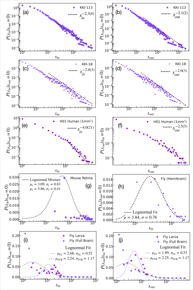
Figure 4: The weighted in and out strengths of source and sink nodes of (a)-(b) KKI-113, (c)-(d) KKI-18, (e)-(f) H01 Human (1mm³), (g) mouse retina (in-strength only), (h) Fly (Hemibrain) (in-strength only) and (i)-(j) Fly (Larva and Full brain).

Each network node’s contributions to the overall design of a brain network can be measured once it has been defined. The network participation indices which Kotter and Stephan studied, showed areas of relatively densely connected nodes that were receiving (referred to as ”receivers”) and emitting (referred to as ”senders”) connections [56]. There are instances when these participatory network metrics they mentioned—like extremely central nodes also have high degree. Information transit may be connected to these network participation metrics [3]. In the following, we explore how the distributions of nodes with purely incoming and outgoing edges contribute to the network.

Table 4 summarizes source (nodes with only outgoing edges) and sink (nodes with only incoming edges) nodes with their corresponding average in or out strengths for all the datasets being considered. For KKI-113, (pure) source, and sink nodes make up approximately 0.84 % and 0.71 % of the network, respectively. On the other hand, KKI-18 is made up of 0.27 % source nodes and 0.29 % sink nodes. The human H01 (mm³) dataset consists of 15.53% source nodes and 15.80% sink nodes. For the non-human connectomes, we find cases of either having little to no source or sink nodes, such as the case of the mouse retina (with only one source node) and a fly hemibrain, both uni- and bidirectional edges dataset, contain only a few sink nodes. This may be due to the fact, that the mouse retina and the fly hemibrain, are only sections of an entire organism’s neuronal network. Notice, however, that although these non-human connectomes have fewer nodes, they have very high connectivity to the rest of their neighbors as indicated by their relatively high average node strengths. Meanwhile, for a fly larva, being only in its developmental stages, the source and sink nodes comprise 0.02% and 0.01% of its entire network. Finally, for the full fruit fly brain, we can observe that its source nodes comprise 6.89 % of its neuronal network, while its sink nodes make up 7.06% of it.

Even though Tables 1 and 4 indicate that these nodes only comprise a small fraction of the networks, some of these nodes serve as hubs, which is evident in the large value of maximum $s_{in}$ and $s_{out}$. Because of this, they can be crucial for neural integration and brain communication, making them important participants in cognitive processes. Furthermore, at times of stress, these network regions are prone to disconnecting and malfunctioning [57]. For example, mapping the locations of sources and sinks in a mouse brain revealed that the prefrontal cortex and other higher-order brain regions are the main neuronal output sources for the rest of the brain, while the basal ganglia are important receivers of incoming projections [58]. In this work, we slightly touch on the topic of source and sink in the neuronal networks of humans (KKI-113, KKI-18), the mouse, and a fruit fly. This time, we explore the mouse retina and investigate the strength distributions of the source and sink nodes. Additionally, as in the case of humans, sources are found to be high-influence nodes which inhibit the sink nodes from going to epileptic seizures [59].Figure 4 shows the probability distributions of the node strengths of the source ($P(s_{out}|s_{in}=0$)) and sink ($P(s_{in}|s_{out}=0$)) nodes in the network datasets being considered.

Interestingly, for the human connectomes KKI-113, KKI-18, and the human H01 (1mm³) datasets, the strength distributions of these sources and sinks follow power-law tails which have exponents slightly above 2. Note that for the strength distribution of the H01 source nodes, find a sharp knee-point (at $s_{in}\approx 11$) in its distribution followed by a steep tail (with exponent $\alpha\approx 4$). This sharp transition can signal finite-size limitations since we are looking into a 1mm³-sized region. However, for the case of non-human connectomes (Figure 4(e)-(h)), we observe lognormal behaviors of source and sink nodes strengths.

Table 5: Source-Sink node strength fitting parameters

Dataset Sources ($s_{in}=0$) Sinks ($s_{out}=0$) Fitting Parameters Fitting Parameters KKI-113 PL $\alpha=2.3(4)$, $D=0.056$ PL $\alpha=2.1(2)$, $D=0.056$ KKI-18 PL $\alpha=2.0(3)$, $D=0.082$ PL $\alpha=2.0(3)$, $D=0.081$ H01 Human (1mm³) PL $\alpha=4.0(21)$, $D=0.039$ PL $\alpha=2.5(5)$, $D=0.075$ Mouse Retina - - Lognormal Mixture $\mu_{1}=3.09$ $\sigma_{1}=0.83$ $\mu_{2}=5.86$ $\sigma_{2}=0.41$ Fly (Hemibrain) [FHB] - - Lognormal $\mu=3.84$ $\sigma=0.76$ Fly (Hemibrain reciprocated) [FHBR] - - - - Fly (Full Brain) [FFB] Lognormal $\mu=2.24$ $\sigma=1.17$ Lognormal $\mu=2.25$ $\sigma=1.17$ Fly (Larva) [FL] Lognormal $\mu=2.68$ $\sigma=0.52$ Lognormal $\mu=1.89$ $\sigma=0.53$

The mouse retina is expectantly smaller with only over a thousand nodes and around half a million edges. By examining the distributions of nodes with either only incoming or outgoing edges, we found that there is only one node in the network that has no incoming edges (identified to be Node $0$ with $s_{0}^{out}=3977$). Such voxel may be part of the retina that is closest to the mouse’s brain which distributes information to all other neighboring nodes in the network. Additionally, looking at the sink nodes, qualitatively it was observed that after the first peak, there is another rise in the trend before it goes down again. Note that events following lognormal behaviors are independent random variables with mean and standard deviation values that are also independent of each other which means that it does not matter how we regroup our data. Having said this, we closely inspect the data by splitting it into two: $s_{in}\leq 97$ and $s_{in}>97$. This value was selected because the intermediate bins are empty signaling a decay of the previous mode and the rise of the second modal curve. Here, we saw that each range of data would follow a lognormal trend and as a whole, the entire dataset follows a bimodal lognormal distribution (or lognormal mixture). Such behavior can model the first-order kinetics of chemicals when mixed [60]. Additionally, the modes of a lognormal mixture represent the subsequent waves of a pandemic [61]. Lastly, it was discovered that the distribution might also represent market volatility structures [62]. In this context, the lognormal mixture observed in the mouse retina dataset implies clustering and differences in the concentration of connections within the mouse retina. Here, we observe that there is a high probability of finding sparsely connected regions; and the occurrence of densely connected portions (with more than 100 incoming edges) of sink nodes. According to earlier research [54], synaptic strengths in the rat visual cortex follow a lognormal distribution with a heavy tail, indicating a higher-than-expected abundance of strong synaptic connections. Furthermore, stronger connections tend to be more heavily clustered [3], which may account for the datapoint concentration at the lognormal mixture’s second peak.

Finally, for the case of the fruit fly datasets (hemibrain, larva, and full brain), the in and out strengths of the source and sink nodes still obey the lognormal behavior, which may be hinted from the behavior of the local weight distributions shown in Figure 3(j)-(l). Similar to the in and out node strength distributions we can still find that the $\mu_{FFB}<\mu_{FL}$ and that $\sigma_{FFB}>\sigma_{FL}$ (shown in Figure 3(m)-(o). We believe that the same underlying mechanisms are responsible for these observations.

4 Possible explanation for PLs of global weight distributions

Long-time learning and memory were shown to be induced via the long-term potentiation (LTP) synaptic plasticity, which is related to the longevity of neighboring neuron pair firing activity [63]. LTP results from coincident activity of pre- and post-synaptic elements, bringing about a facilitation of chemical transmission, that can persist for periods of weeks or months.

At criticality the distribution of a single node activity duration time $P(t_{A})$ can be expressed as follows

$$\int_{t_{A}}^{\infty}P(t_{A})\mathrm{d}t=C_{AA}(t_{A})\,,$$ (3)

via the auto-correlation function $C_{AA}(t_{A})\propto t_{A}^{-\lambda/Z}$, where $\lambda$ is the auto-correlation exponent, and $Z$ is the dynamical exponent of the critical process [64]. This gives rise to $P(t_{A})\sim t_{A}^{-\tau_{t}}=t_{A}^{-\lambda/Z-1}$ and the exponent relation $\tau_{t}=\lambda/Z+1$. For a generic universality class considered to describe brain criticality [17], the Directed Percolation (DP) in the mean-field limit the auto-correlation function decays asymptotically as $t^{-\lambda/Z}=t^{-4}$ [65], thus $\tau_{t}=5$ could be expected. In $d=2$ spatial dimensions this is $\lambda/Z=2.5(3)$ [65], providing an estimate $\tau_{t}=3.5(3)$ for the DP class.

However, it is still an open question if the critical brain would belong to the mean-field DP universality class or to other and if non-universal scaling [66, 67], corresponding to a Griffiths phase [68] or to an external drive [69, 70]. In the case of the Shinomoto-Kuramoto model, possessing periodic external forces, to describe the task phase of the fruit-fly brain it was shown that PDF-s of the activation periods decay with non-universal power-laws characterized by exponents $\tau_{t}\simeq 2$, depending on the strength of the excitation [70]. Similar behavior was found for the Hurst and beta exponents, which describe auto-correlations. A community dependence has also been confirmed via fMRI and BOLD signal measurements [71] for humans.

Thus, assuming that synaptic weights $w_{ij}$, obtained by LTP, are proportional with the activity duration times $\tau_{AA}\sim\tau_{A}$ we can expect that their probability distributions exhibit the same PL tails characterized by $\tau_{t}$.

5 Summary

In summary, we have investigated the weight distributions of various human and animal connectomes, to search for power-law-tailed PDFs, which can be related to the learning mechanism of the brain in a critical state. These are the largest, publicly available neural graphs. We found that the global weight distributions can be fitted by PL tails, characterized by exponents slightly above 3, the node strength PDF-s decay faster, stretched exponentially, or via log-normal way. The whole brain human fiber tracks, obtained by MRI with deterministic tractography, using the Fiber Assignment by Continuous Tracking algorithm methods [72] exhibit the most PL-like behavior, even the node strengths of the source and sink nodes are like that.

We have compared these results of adult (human and animal) connectomes with that of an untrained, larva fly and found that the latter has a narrow PDF, that starts in the same way as the adult fly. This suggests that a certain degree of learning happens already in premature brain development or the initial axon growth mechanisms could also lead to fat tails in the connection strengths [6]. This should be studied more, using other connectomes obtained in the early phase of neural growth.

We provided a possible model and a scaling relation, which connects the critical auto-correlation function to the LTF plasticity mechanism, that can explain the PL-s we observe. Thus we rely on the mutual relationship between structural and functional connectomes and claim that non-local learning is dictated by a brain state close to criticality. But in the lack of the true whole-brain function model, we can’t give a precise exponent estimate.

Finally, we have also determined the white matter fiber tract distance distributions of the large KKI-113 human connectome. We found that it follows the exponential rule up to centimeter size, but breaks down and decays faster for longer lengths. Note, that the distances are calculated from the x,y, and z coordinates of nodes as we don’t know the real wire lengths.

Data availability

The fitted data currently available for a request from the authors.

6 Supplementary Materials

In this section, we present in detail the methods (i.e.binning, statistical fitting) employed in our analyses.

6.1 Data Binning

6.1.1 The Logarithmic and Linear Binning

In this work, we employed both linear and logarithmic binning to our data. We did this because we are dealing with datasets of varying sizes. Figure 5 shows a schematic of the log binning employed.

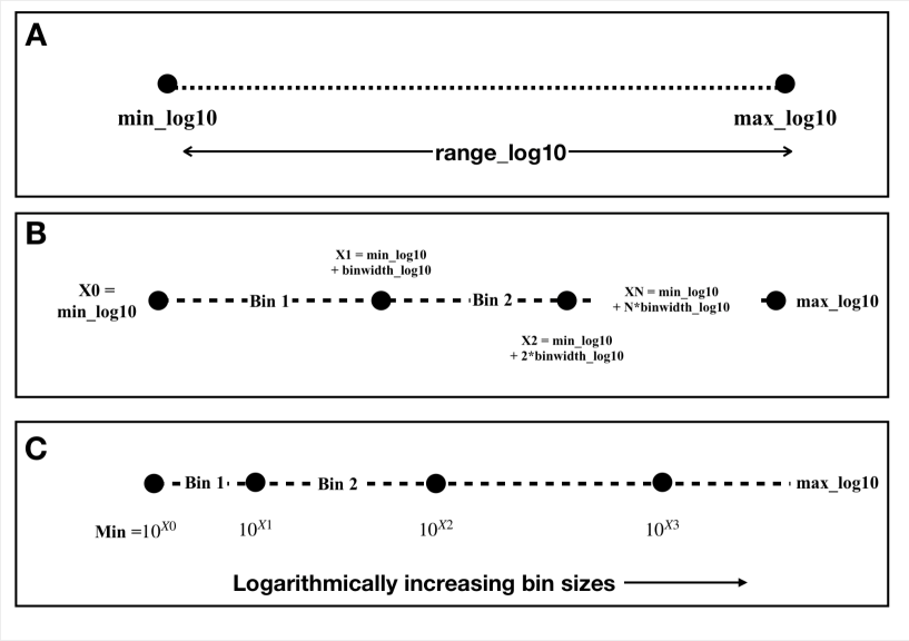
Figure 5: Schematic of Logarithmic Binning. (a) To be equally spaced in the log scale, the range of the data is defined by taking the difference of the log of the minimum and maximum of data (b) The range of data is divided by the number of bins set. The more data points, the larger the number of bins (c) How it looks like in the linear scale.

Since the datasets vary in size, the number of bins set also varies. In general, the number of bins set ensures that there are no empty bins to avoid erratic trends. The choice of binning, either linear or logarithmic, is based on the number of data points $N$ and maximum value. For the case of linear binning, the same schematics apply except that we don’t take the log of the data points.

In the following, we listed the type of binning employed for every dataset presented in the main text.

6.1.2 Global weights distribution

Table 6: Summary of global weights data and employed binning

Dataset	Number of datapoints, $N$	Max. value	Type of binning
KKI-113	48,096,501	1,377.0	Logarithmic
KKI-18	46,524,003	854.0	Logarithmic
H01 Human (1mm3)	76, 004	89	Logarithmic
Mouse Retina	577,350	29.0	Linear
Fly (Hemibrain)	3,413,160	4,299.0	Logarithmic
Fly (Hemibrain reciprocated)	3,251,362	4,299	Logarithmic
Fly (Full brain)	3,794,527	2,358.0	Logarithmic
Fly (Larva)	110,677	121.0	Linear

6.1.3 Local node strengths distribution

Table 7: Summary of node in-strength data and employed binning

Dataset	Number of datapoints, $N$	Max. value	Type of binning
KKI-113	1,598,266	4,977.0	Logarithmic
KKI-18	752,358	38,243.0	Logarithmic
H01 Human (1mm3)	13,579	94	Logarithmic
Mouse Retina	1,076	5,000.0	Linear
Fly (Hemibrain)	21,662	2,708.0	Logarithmic
Fly (Hemibrain reciprocated)	16,804	4224.0	Logarithmic
Fly (Full brain)	124,778	23,036.0	Logarithmic
Fly (Larva)	2,952	210.0	Linear

Table 8: Summary of node out-strength data and employed binning

Dataset	Number of datapoints, $N$	Max. value	Type of binning
KKI-113	1,598,266	5,010.0	Logarithmic
KKI-18	749,667	55, 441.0	Logarithmic
H01 Human (1mm3)	13, 579	95.0	Logarithmic
Mouse Retina	1, 076	6,880.0	Linear
Fly (Hemibrain)	21, 662	5,044.0	Logarithmic
Fly (Hemibrain reciprocated)	16,804	4,378.0	Logarithmic
Fly (Full brain)	124,778	12,898.0	Logarithmic
Fly (Larva)	2, 952	160.0	Linear

Table 9: Summary of node total (in + out) node strength data and employed binning

Dataset	Number of datapoints, $N$	Max. value	Type of binning
KKI-113	1,598,266	6, 285.0	Logarithmic
KKI-18	797, 759	73, 451.0	Logarithmic
H01 Human (1mm3)	13, 579	159.0	Logarithmic
Mouse Retina	1, 076	7, 853.0	Linear
Fly (Hemibrain)	21, 662	7,511.0	Logarithmic
Fly (Hemibrain reciprocated)	16,804	6,394.0	Logarithmic
Fly (Full brain)	124,778	26, 593.0	Logarithmic
Fly (Larva)	2, 952	331.0	Linear

Table 10: Summary of source and sink node strength data and employed binning

Dataset Sources $s_{in}=0$ Sinks $s_{out}=0$ Type of binning No. of datapoints, $N$ Max. value No. of datapoints, N Max. value KKI-113 6684 2110.0 5,686 536 Logarithmic KKI-18 2270 1663.0 2,410 1,300 Logarithmic H01 Human (1mm³) 2,109 42 2,145 42 Logarithmic Mouse Retina 1 3977.0 61 913 Linear (sinks only) Fly (Hemibrain) - - 46 250 Linear Fly (Hemibrain reciprocated) 3 17.0 1 3 - Fly (Full Brain) 8,565 640.0 8,809 766 Logarithmic Fly (Larva) 58 18.0 43 38 Linear

6.2 The Power-Law

Functional brain networks have been proposed to exhibit scale-free behaviors with power-laws present [12, 13]. Power-laws indicate a specific degree of self-organization, either by growth and preferred attachment or replication, as in biological/metabolic networks [14, 15]. When there is a transition from an ordered to an unordered phase without a characteristic length scale, power laws play a crucial role in statistical physics. Both theoretical and practical data support the notion that the brain functions near this important area [19, 20, 18, 17].

The power-law is of the form

$$P(x)=Cx^{-\alpha}$$ (4)

where $C$ is the scaling factor, and $\alpha$ is the power-law exponent. In this work, we fitted our data (Figure 2 and Figure 4) by employing the methods of Clauset et.al. [44] implemented by Alstott in Python [73].

For an integer variable (such as the number of edges emanating from a node), the power-law can be expressed as

$$P(x)=\frac{x^{-\alpha}}{\zeta(\alpha,x_{min})}$$ (5)

where $\zeta(\alpha,x_{min})$ is the generalized Hurwitz zeta function [44] given by the expression,

$$\zeta(\alpha,x_{min})=\frac{(x_{min}-\frac{1}{2})^{-\alpha+1}}{\alpha-1}\left[1+\mathcal{O}(x_{min}^{-2})\right]$$ (6)

As the power-law exponent may vary depending on the range of data being fitted (as sometimes only a region display a linear trend on the log-log space), we also computed for the Kolmogorov-Smirnov distance $D$,

$$D_{\alpha}=max_{x}|P_{empirical}(x)-P(x)_{\alpha}|$$ (7)

where $P_{empirical}(x)$ and $P(x)_{\alpha}$ denote the cumulative density functions of the data and the power law with exponent $\alpha$.

Additionally, we also computed the marginal error of our power-law fit, for the discrete case, we have

$$\sigma=\frac{1}{\sqrt{N\left[\frac{\zeta^{\prime\prime}(\alpha,x)}{\zeta(\alpha,x)}-\left(\frac{\zeta^{\prime}(\alpha,x)}{\zeta(\alpha,x)}\right)^{2}\right]}}$$ (8)

where $N$ is the number of datapoints and $\alpha$ is the powerlaw exponent.

6.3 The Stretched Exponential

To account quantitatively for many reported natural fat tail distributions in nature and economy, Laherrere and Sornette [46] proposed the stretched exponential 9 as an alternative to the power-law.

$$P(x)dx=c\left(\frac{x^{c-1}}{A_{o}^{c}}\right)e^{\left[(\frac{-x}{A_{o}})^{c}\right]}dx$$ (9)

such that the cumulative distribution is

$$P_{c}(x)=e^{\left[(\frac{-x}{A_{o}})^{c}\right]}$$ (10)

Stretched exponentials are characterized by an exponent $c<1$, in which the exponent $c$ is the inverse of the number of generations (or products) in a multiplicative process. The borderline $c=1$ corresponds to the usual exponential distribution. For $c<1$, the distribution 10 presents a clear curvature in a log-log plot while exhibiting a relatively large apparent linear behavior, all the more so, the smaller $c$ is. It can thus be used to account both for a limited scaling regime and a cross-over to non-scaling. When using the stretched exponential pdf, the rationale is that the deviations from a power law description are fundamental and not only a finite-size correction.

Among its numerous benefits is its economy—it has only two movable parameters with definite physical meaning. Moreover, it originates from a straightforward and universal mechanism concerning multiplicative processes.

To find the fitting for the in, out, and total strength distributions, here I computed for the best fitting parameters $A_{o}$ and $c$ (exponent) of the stretched exponential by using the mean and standard deviation of the data and scanning through a range of values for $c$ (from 0.1 to 0.9999).

Adapting from the Appendix section of [46], this section shows the derivation of the condition for the data to follow a stretched exponential. We start with the mean of the stretched exponential 9 given by

$$<x>=x_{o}\left(\frac{1}{c_{o}}\right)\Gamma\left(\frac{1}{c_{o}}\right)$$ (11)

and its variance is

$$\sigma^{2}=x_{o}^{2}\left(\frac{2}{c_{o}}\right)\Gamma\left(\frac{2}{c_{o}}\right)-<x>^{2}$$ (12)

From  11:

$$x_{o}=\frac{c_{o}<x>}{\Gamma\left(\frac{1}{c_{o}}\right)}$$ (13)

Plug-in 13 to  12 we get:

$$\sigma^{2}=\frac{c_{o}^{2}<x>^{2}}{\Gamma^{2}\left(\frac{1}{c_{o}}\right)}\left(\frac{2}{c_{o}}\right)\Gamma\left(\frac{2}{c_{o}}\right)-<x>^{2}$$ (14)

Simplifying 14 by factoring out $<x>$ we get,

$$\sigma^{2}=\left[2c_{o}\frac{\Gamma\left(\frac{2}{c_{o}}\right)}{\Gamma\left(\frac{1}{c_{o}}\right)}-1\right]<x>^{2}$$ (15)

Transpose $<x>^{2}$ to the other side,

$$\frac{\sigma^{2}}{<x>^{2}}=\left[2c_{o}\frac{\Gamma\left(\frac{2}{c_{o}}\right)}{\Gamma\left(\frac{1}{c_{o}}\right)}-1\right]$$ (16)

Add 1 to both sides of 16,

$$\frac{\sigma^{2}}{<x>^{2}}+1=\left[2c_{o}\frac{\Gamma\left(\frac{2}{c_{o}}\right)}{\Gamma\left(\frac{1}{c_{o}}\right)}\right]$$ (17)

Divide everything by 2 and rearrange,

$$\left[c_{o}\frac{\Gamma\left(\frac{2}{c_{o}}\right)}{\Gamma\left(\frac{1}{c_{o}}\right)}\right]=\frac{\sigma^{2}}{2<x>^{2}}+\frac{1}{2}$$ (18)

If we let the LHS of 18 be,

$$F_{o}=\left[c_{o}\frac{\Gamma\left(\frac{2}{c_{o}}\right)}{\Gamma\left(\frac{1}{c_{o}}\right)}\right]$$ (19)

and the RHS be some constant $F_{o}$ which is a function of $\sigma$, the standard deviation and $<x>$ is the mean of the data.

$$F=\frac{\sigma^{2}}{2<x>^{2}}+\frac{1}{2}$$ (20)

Here, if the conditions $f=|F-F_{o}|=0$ and $c<1$ are met, then the data follow a stretched exponential trend.

6.4 The Exponential Truncated Power-Law

In this work, we used the exponential truncated power-law of the form

$$P(x)=C(x+x_{o})^{-\beta}\;\exp(-x/\kappa)$$ (21)

from the work of Gonzalez and Barabási [74]. Simply put, an exponentially truncated power-law is a power law multiplied by an exponential function. Since they applied this to displacements $r$ in cities, we replaced the variable $r$ with $x$ to make it into a more general form. Here, the parameter $\beta$ is the power-law exponent that is valid for small values of $s$, and $\kappa$ is the cut-off value. To determine the fitting parameters $s_{o}$, $\beta$, and $\kappa$, we employed the curve_fit() function from Python’s scipy.stats. To check the goodness-of-fit of our data to the said distribution, we compute for the $R^{2}$ value, defined as

$$R^{2}=1-\frac{SS_{res}}{SS_{tot}}$$ (22)

where $SS_{res}$ is the residual sum of squares

$$SS_{res}=\sum_{i}(y_{i}-f_{i})^{2}$$ (23)

where $y_{i}$ is the observed data associated with a fitted or predicted value $f_{i}$. On the other hand, the total sum of squares $SS_{tot}$ is given by

$$SS_{res}=\sum_{i}(y_{i}-\bar{y})^{2}$$ (24)

where $\bar{y}$ is the mean of the data.

6.5 The Lognormal Distribution

Based on earlier research [54], synaptic strengths in the rat visual cortex follow a lognormal distribution with a heavy tail, indicating a higher-than-expected abundance of strong synaptic connections. Here, we opted to fit the node strength distributions of the mouse retina with a lognormal distribution as well.

The lognormal distribution is a continuous probability distribution of a random variable whose logarithm is normally distributed. A log-normal process is the statistical realization of the multiplicative product of many independent random variables, each of which is positive.

$$P(x)=\frac{1}{x\sigma\sqrt{2\pi}}\exp\left(\frac{-(ln\;x-\mu)^{2}}{2\sigma^{2}}\right)$$ (25)

where $\mu$ is the expected value (or mean) and $\sigma$ is the standard deviation of the variable’s natural logarithm, not the expectation and standard deviation of observed variable $x$ itself.

$$\mu=ln\;\left(\frac{\mu_{x}^{2}}{\sqrt{\mu_{x}^{2}+\sigma^{2}}}\right)$$ (26)

$$\sigma=ln\;\left(1+\frac{\sigma_{x}^{2}}{\mu_{x}^{2}}\right)$$ (27)

where $\mu_{x}$ and $\sigma_{x}$ are the mean and standard deviation of the data.

References

- [1] Dániel L Barabási, Ginestra Bianconi, Ed Bullmore, Mark Burgess, SueYeon Chung, Tina Eliassi-Rad, Dileep George, István A Kovács, Hernán Makse, Thomas E Nichols, et al. Neuroscience needs network science. Journal of Neuroscience, 43(34):5989–5995, 2023.
- [2] William B Kristan and Paul Katz. Form and function in systems neuroscience. Current biology, 16(19):R828–R831, 2006.
- [3] Olaf Sporns. Networks of the Brain. MIT press, 2016.
- [4] Valentino Braitenberg and Almut Schüz. Cortex: statistics and geometry of neuronal connectivity. Springer Science & Business Media, 2013.
- [5] Raymond L Beurle. Properties of a mass of cells capable of regenerating pulses. Philosophical Transactions of the Royal Society of London. Series B, Biological Sciences, pages 55–94, 1956.
- [6] Christopher W. Lynn, Caroline M. Holmes, and Stephanie E. Palmer. Heavy-tailed neuronal connectivity arises from hebbian self-organization. Nature Physics, 20(3):484–491, Mar 2024.
- [7] Anastasiya Salova and István A Kovács. Combined topological and spatial constraints are required to capture the structure of neural connectomes. arXiv preprint arXiv:2405.06110, 2024.
- [8] Mária Ercsey-Ravasz, Nikola T Markov, Camille Lamy, David C Van Essen, Kenneth Knoblauch, Zoltán Toroczkai, and Henry Kennedy. A predictive network model of cerebral cortical connectivity based on a distance rule. Neuron, 80(1):184–197, 2013.
- [9] Michael T Gastner and Géza Ódor. The topology of large open connectome networks for the human brain. Scientific reports, 6(1):27249, 2016.
- [10] Géza Ódor. Critical dynamics on a large human open connectome network. Physical Review E, 94(6):062411, 2016.
- [11] Géza Ódor, Gustavo Deco, and Jeffrey Kelling. Differences in the critical dynamics underlying the human and fruit-fly connectome. Physical Review Research, 4(2):023057, 2022.
- [12] Victor M Eguiluz, Dante R Chialvo, Guillermo A Cecchi, Marwan Baliki, and A Vania Apkarian. Scale-free brain functional networks. Physical review letters, 94(1):018102, 2005.
- [13] Martijn P van den Heuvel, Cornelis J Stam, Maria Boersma, and HE Hulshoff Pol. Small-world and scale-free organization of voxel-based resting-state functional connectivity in the human brain. Neuroimage, 43(3):528–539, 2008.
- [14] Albert-László Barabási and Réka Albert. Emergence of scaling in random networks. science, 286(5439):509–512, 1999.
- [15] Filip Piekniewski. Robustness of power laws in degree distributions for spiking neural networks. In 2009 International Joint Conference on Neural Networks, pages 2541–2546. IEEE, 2009.
- [16] Riccardo Zucca, Xerxes D Arsiwalla, Hoang Le, Mikail Rubinov, Antoni Gurguí, and Paul Verschure. The degree distribution of human brain functional connectivity is generalized pareto: A multi-scale analysis. BioRxiv, page 840066, 2019.
- [17] John M Beggs and Dietmar Plenz. Neuronal avalanches in neocortical circuits. Journal of neuroscience, 23(35):11167–11177, 2003.
- [18] Claus-C Hilgetag, Gully APC Burns, Marc A O’Neill, Jack W Scannell, and Malcolm P Young. Anatomical connectivity defines the organization of clusters of cortical areas in the macaque and the cat. Philosophical Transactions of the Royal Society of London. Series B: Biological Sciences, 355(1393):91–110, 2000.
- [19] Woodrow L Shew and Dietmar Plenz. The functional benefits of criticality in the cortex. The neuroscientist, 19(1):88–100, 2013.
- [20] Ariel Haimovici, Enzo Tagliazucchi, Pablo Balenzuela, and Dante R Chialvo. Brain organization into resting state networks emerges at criticality on a model of the human connectome. Physical Review Letters, 110(17):178101, 2013.
- [21] Gerald Hahn, Adrian Ponce-Alvarez, Cyril Monier, Giacomo Benvenuti, Arvind Kumar, Frédéric Chavane, Gustavo Deco, and Yves Frégnac. Spontaneous cortical activity is transiently poised close to criticality. PLOS Computational Biology, 13:1–29, 05 2017.
- [22] Olaf Sporns, Giulio Tononi, and Rolf Kötter. The human connectome: a structural description of the human brain. PLoS computational biology, 1(4):e42, 2005.
- [23] Bennett A Landman, Alan J Huang, Aliya Gifford, Deepti S Vikram, Issel Anne L Lim, Jonathan AD Farrell, John A Bogovic, Jun Hua, Min Chen, Samson Jarso, et al. Multi-parametric neuroimaging reproducibility: a 3-t resource study. Neuroimage, 54(4):2854–2866, 2011.
- [24] Céline Delettre, Arnaud Messé, Leigh-Anne Dell, Ophélie Foubet, Katja Heuer, Benoit Larrat, Sebastien Meriaux, Jean-Francois Mangin, Isabel Reillo, Camino de Juan Romero, et al. Comparison between diffusion mri tractography and histological tract-tracing of cortico-cortical structural connectivity in the ferret brain. Network Neuroscience, 3(4):1038–1050, 2019.
- [25] Open connectome project, 2015. https://neurodata.io.
- [26] Michael T. Gastner and Géza Ódor. The topology of large Open Connectome networks for the human brain. Scientific Reports, 6(1):27249, June 2016.
- [27] Flywire connectome data, 2023. https://codex.flywire.ai/api/download.
- [28] The hemibrain dataset (v1.0.1), 2020.
- [29] Michael Winding, Benjamin D. Pedigo, Christopher L. Barnes, Heather G. Patsolic, Youngser Park, Tom Kazimiers, Akira Fushiki, Ingrid V. Andrade, Avinash Khandelwal, Javier Valdes-Aleman, Feng Li, Nadine Randel, Elizabeth Barsotti, Ana Correia, Richard D. Fetter, Volker Hartenstein, Carey E. Priebe, Joshua T. Vogelstein, Albert Cardona, and Marta Zlatic. The connectome of an insect brain. Science, 379(6636):eadd9330, 2023.
- [30] 2024. https://neurodata.io/project/connectomes.
- [31] Alain Barrat, Marc Barthelemy, Romualdo Pastor-Satorras, and Alessandro Vespignani. The architecture of complex weighted networks. Proceedings of the national academy of sciences, 101(11):3747–3752, 2004.
- [32] Yong-Yeol Ahn, Hawoong Jeong, and Beom Jun Kim. Wiring cost in the organization of a biological neuronal network. Physica A: Statistical Mechanics and its Applications, 367:531–537, 2006.
- [33] Ed Bullmore and Olaf Sporns. The economy of brain network organization. Nature reviews neuroscience, 13(5):336–349, 2012.
- [34] Beth L Chen, David H Hall, and Dmitri B Chklovskii. Wiring optimization can relate neuronal structure and function. Proceedings of the National Academy of Sciences, 103(12):4723–4728, 2006.
- [35] Longchuan Li, James K Rilling, Todd M Preuss, Matthew F Glasser, Frederick W Damen, and Xiaoping Hu. Quantitative assessment of a framework for creating anatomical brain networks via global tractography. NeuroImage, 61(4):1017–1030, 2012.
- [36] Van J Wedeen, RP Wang, Jeremy D Schmahmann, Thomas Benner, Wen-Yih Isaac Tseng, Guangping Dai, Deepak N Pandya, Patric Hagmann, Helen D’Arceuil, and Alex J de Crespigny. Diffusion spectrum magnetic resonance imaging (dsi) tractography of crossing fibers. Neuroimage, 41(4):1267–1277, 2008.
- [37] Saad Jbabdi and Heidi Johansen-Berg. Tractography: where do we go from here? Brain connectivity, 1(3):169–183, 2011.
- [38] Holger Finger, Marlene Bönstrup, Bastian Cheng, Arnaud Messé, Claus Hilgetag, Götz Thomalla, Christian Gerloff, and Peter König. Modeling of large-scale functional brain networks based on structural connectivity from dti: comparison with eeg derived phase coupling networks and evaluation of alternative methods along the modeling path. PLoS computational biology, 12(8):e1005025, 2016.
- [39] P Thomas Schoenemann, Michael J Sheehan, and L Daniel Glotzer. Prefrontal white matter volume is disproportionately larger in humans than in other primates. Nature neuroscience, 8(2):242–252, 2005.
- [40] Jan Karbowski. Global and regional brain metabolic scaling and its functional consequences. BMC biology, 5:1–11, 2007.
- [41] James L Ringo, Robert W Doty, Steven Demeter, and Patrice Y Simard. Time is of the essence: a conjecture that hemispheric specialization arises from interhemispheric conduction delay. Cerebral Cortex, 4(4):331–343, 1994.
- [42] Kimberley A Phillips, Cheryl D Stimpson, Jeroen B Smaers, Mary Ann Raghanti, Bob Jacobs, Anastas Popratiloff, Patrick R Hof, and Chet C Sherwood. The corpus callosum in primates: processing speed of axons and the evolution of hemispheric asymmetry. Proceedings of the Royal Society B: Biological Sciences, 282(1818):20151535, 2015.
- [43] Jesse Tinker and Jose Luis Perez Velazquez. Power law scaling in synchronization of brain signals depends on cognitive load. Frontiers in systems neuroscience, 8:73, 2014.
- [44] Aaron Clauset, Cosma Rohilla Shalizi, and Mark EJ Newman. Power-law distributions in empirical data. SIAM review, 51(4):661–703, 2009.
- [45] Stefano Mossa, Marc Barthelemy, H Eugene Stanley, and Luis A Nunes Amaral. Truncation of power law behavior in “scale-free” network models due to information filtering. Physical Review Letters, 88(13):138701, 2002.
- [46] Jean Laherrere and Didier Sornette. Stretched exponential distributions in nature and economy:“fat tails” with characteristic scales. The European Physical Journal B-Condensed Matter and Complex Systems, 2:525–539, 1998.
- [47] Jordan Grafman. Conceptualizing functional neuroplasticity. Journal of communication disorders, 33(4):345–356, 2000.
- [48] Richard J Davidson and Bruce S McEwen. Social influences on neuroplasticity: stress and interventions to promote well-being. Nature neuroscience, 15(5):689–695, 2012.
- [49] Bruce S McEwen. Redefining neuroendocrinology: epigenetics of brain-body communication over the life course. Frontiers in Neuroendocrinology, 49:8–30, 2018.
- [50] James D Jontes and Stephen J Smith. Filopodia, spines, and the generation of synaptic diversity. Neuron, 27(1):11–14, 2000.
- [51] Luıs A Nunes Amaral, Antonio Scala, Marc Barthelemy, and H Eugene Stanley. Classes of small-world networks. Proceedings of the national academy of sciences, 97(21):11149–11152, 2000.
- [52] Roger Guimera, Stefano Mossa, Adrian Turtschi, and LA Nunes Amaral. The worldwide air transportation network: Anomalous centrality, community structure, and cities’ global roles. Proceedings of the National Academy of Sciences, 102(22):7794–7799, 2005.
- [53] Daniel J Felleman and David C Van Essen. Distributed hierarchical processing in the primate cerebral cortex. Cerebral cortex (New York, NY: 1991), 1(1):1–47, 1991.
- [54] Sen Song, Per Jesper Sjöström, Markus Reigl, Sacha Nelson, and Dmitri B Chklovskii. Highly nonrandom features of synaptic connectivity in local cortical circuits. PLoS biology, 3(3):e68, 2005.
- [55] Sven Dorkenwald, Arie Matsliah, Amy R Sterling, Philipp Schlegel, Szi-chieh Yu, Claire E. McKellar, Albert Lin, Marta Costa, Katharina Eichler, Yijie Yin, Will Silversmith, Casey Schneider-Mizell, Chris S. Jordan, Derrick Brittain, Akhilesh Halageri, Kai Kuehner, Oluwaseun Ogedengbe, Ryan Morey, Jay Gager, Krzysztof Kruk, Eric Perlman, Runzhe Yang, David Deutsch, Doug Bland, Marissa Sorek, Ran Lu, Thomas Macrina, Kisuk Lee, J. Alexander Bae, Shang Mu, Barak Nehoran, Eric Mitchell, Sergiy Popovych, Jingpeng Wu, Zhen Jia, Manuel Castro, Nico Kemnitz, Dodam Ih, Alexander Shakeel Bates, Nils Eckstein, Jan Funke, Forrest Collman, Davi D. Bock, Gregory S.X.E. Jefferis, H. Sebastian Seung, Mala Murthy, and . Neuronal wiring diagram of an adult brain. bioRxiv, 2023.
- [56] Rolf Kötter and Klaas E Stephan. Network participation indices: characterizing component roles for information processing in neural networks. Neural Networks, 16(9):1261–1275, 2003.
- [57] Martijn P Van den Heuvel and Olaf Sporns. Network hubs in the human brain. Trends in cognitive sciences, 17(12):683–696, 2013.
- [58] Ludovico Coletta, Marco Pagani, Jennifer D Whitesell, Julie A Harris, Boris Bernhardt, and Alessandro Gozzi. Network structure of the mouse brain connectome with voxel resolution. Science advances, 6(51):eabb7187, 2020.
- [59] Kristin M Gunnarsdottir, Adam Li, Rachel J Smith, Joon-Yi Kang, Anna Korzeniewska, Nathan E Crone, Adam G Rouse, Jennifer J Cheng, Michael J Kinsman, Patrick Landazuri, et al. Source-sink connectivity: A novel interictal eeg marker for seizure localization. Brain, 145(11):3901–3915, 2022.
- [60] August Andersson. Mechanisms for log normal concentration distributions in the environment. Scientific reports, 11(1):16418, 2021.
- [61] Paolo S Valvo. A bimodal lognormal distribution model for the prediction of covid-19 deaths. Applied Sciences, 10(23):8500, 2020.
- [62] Damiano Brigo and Fabio Mercurio. Lognormal-mixture dynamics and calibration to market volatility smiles. International Journal of Theoretical and Applied Finance, 5(04):427–446, 2002.
- [63] S. F. Cooke and T. V. P. Bliss. Plasticity in the human central nervous system. Brain, 129(7):1659–1673, 05 2006.
- [64] G. Ódor. Universality in nonequilibrium lattice systems: Theoretical foundations. World Scientific, 2008.
- [65] Malte Henkel, Haye Hinrichsen, and Sven Lübeck. Non-equilibrium phase transitions, volume 1. Springer, 2008.
- [66] Miguel A. Muñoz. Colloquium: Criticality and dynamical scaling in living systems. Rev. Mod. Phys., 90:031001, Jul 2018.
- [67] Géza Ódor, Michael T Gastner, Jeffrey Kelling, and Gustavo Deco. Modelling on the very large-scale connectome. Journal of Physics: Complexity, 2(4):045002, oct 2021.
- [68] Robert B. Griffiths. Nonanalytic Behavior Above the Critical Point in a Random Ising Ferromagnet. Phys. Rev. Lett., 23(1):17–19, July 1969.
- [69] Daniel J. Korchinski, Javier G. Orlandi, Seung-Woo Son, and Jörn Davidsen. Criticality in spreading processes without timescale separation and the critical brain hypothesis. Phys. Rev. X, 11:021059, Jun 2021.
- [70] Géza Ódor, István Papp, Shengfeng Deng, and Jeffrey Kelling. Synchronization transitions on connectome graphs with external force. Frontiers in Physics, 11, March 2023.
- [71] Jeremi K. Ochab, Marcin Watorek, Anna Ceglarek, Magdalena Fafrowicz, Koryna Lewandowska, Tadeusz Marek, Barbara Sikora-Wachowicz, and Pawel Oswiecimka. Task-dependent fractal patterns of information processing in working memory. Scientific Reports, 12(1), October 2022.
- [72] Susumu Mori, Barbara J Crain, Vadappuram P Chacko, and Peter CM Van Zijl. Three-dimensional tracking of axonal projections in the brain by magnetic resonance imaging. Annals of Neurology: Official Journal of the American Neurological Association and the Child Neurology Society, 45(2):265–269, 1999.
- [73] Jeff Alstott, Ed Bullmore, and Dietmar Plenz. powerlaw: a python package for analysis of heavy-tailed distributions. PloS one, 9(1):e85777, 2014.
- [74] Marta C Gonzalez, Cesar A Hidalgo, and Albert-Laszlo Barabasi. Understanding individual human mobility patterns. nature, 453(7196):779–782, 2008.