Quantum null energy condition in quenched 2d CFTs

Abstract

The quantum null energy condition (QNEC) is a lower bound on the expectation value of the null-null component of the energy-momentum tensor in terms of null variations of the entanglement entropy. A stronger version of the QNEC (the primary QNEC) is expected to hold in $1+1$ dimensional conformal field theories (CFT). QNEC has been shown to impose non-trivial quantum thermodynamic restrictions on irreversible entropy production in quenches in $1+1$ dimensional holographic CFTs. It is therefore natural to study if QNEC imposes similar bounds in other quench setups. In this paper we study QNEC in the Calabrese-Cardy global and local joining quenches using standard CFT techniques. In the global quench we show that the primary QNEC must hold at sufficiently early times and find that it imposes bounds on the four point correlators of twist fields in a boundary state. This is a constraint on the set of boundary states that satisfy the primary QNEC. Furthermore, we find that a violation of the primary QNEC implies a violation of the averaged null energy condition (ANEC) in a conformally transformed frame. In the local quench we find similar bounds on four point correlators from both the primary and the usual QNEC.

1 Introduction

Quantum information theory has played a crucial role in unraveling many aspects of the structure of quantum field theory and quantum gravity Faulkner:2022mlp . One interesting recent development has been the quantum null energy condition (QNEC), a quasi-local lower bound on the energy-momentum tensor in Poincaré invariant quantum field theories (QFT). A very general information-theoretic argument for QNEC was presented in Wall:2017blw . The argument is essentially captured by Landauer’s proclamation that information is physical Landauer:1961 ; Landauer:1991 , i.e., some minimum energy is required to store (erase) a given amount of information Reeb_2014 .

QNEC was first conjectured as a special non-gravitational ($G_{N}$-independent) limit of the Quantum Focusing Conjecture Bousso:2015mna . It has been proven for free quantum field theories (QFTs) Bousso:2015wca ; Malik:2019dpg , holographic QFTs with AdS duals Koeller:2015qmn , and for general Poincaré-invariant QFTs Balakrishnan:2017bjg . More rigorous proofs using half-sided modular inclusion properties of operator algebras have also been provided Ceyhan:2018zfg ; Hollands:2025glm .

It is interesting to ask if QNEC imposes non-trivial constraints on the dynamics of out-of-equilibrium many-body systems described by QFTs. In earlier work Kibe:2021qjy ; Banerjee:2022dgv ; Kibe:2024icu , we found that non-violation of the QNEC imposes upper and lower bounds on irreversible entropy production after a global quench in holographic conformal field theories (CFT). These bounds were argued to be a non-trivial generalization of the classical second law of thermodynamics and were already expected from general quantum information theory arguments PhysRevLett.105.170402 . It is therefore natural to investigate QNEC in a variety of other quenches and examine the bounds imposed on these quenches.

This paper describes results of calculations of the QNEC for quenches in $1+1$ dimensional CFTs. The QNEC is Bousso:2015mna

$$Q_{\pm}\coloneqq 2\pi\langle T_{\pm\pm}\rangle-\partial_{\pm}^{2}S_{\rm EE}\geq 0,$$ (1)

where $\langle T_{\pm\pm}\rangle$ is the expectation value of the two non-zero components of the energy-momentum tensor of the CFT at an arbitrary spacetime point $p$ with $+(-)$ denoting the future directed right (left) moving null directions, $S$ is the entanglement entropy of any spacelike interval with one end-point at $p$, and $\partial_{\pm}S$ is the rate of change of entropy when the end-point $p$ is deformed along the $\pm$ directions while the other end-point is kept fixed.

In $1+1$-dimensional CFTs, a stronger QNEC,

$$\mathcal{Q}_{\pm}\coloneq 2\pi\langle T_{\pm\pm}\rangle-\left(\partial_{\pm}^{2}S+\frac{6}{c}\left(\partial_{\pm}S\right)^{2}\right)\geq 0,$$ (2)

is implied by the inequality (1) Bousso:2015mna ; Wall:2011kb . The argument for this stronger inequality is as follows. The quantity $\mathcal{Q}_{\pm}$ transforms like a conformal primary and one can transform to a conformal frame where the $\partial_{+}S$ term vanishes. The transformation $y\to f(y)$ that achieves this can be found by solving

$$S^{\prime}(f)=f^{\prime}(y)^{-2}\left(\frac{c}{12}S^{\prime}(y)+\frac{f^{\prime\prime}(y)}{f^{\prime}(y)}\right)=0.$$ (3)

The QNEC (1) must hold in this new frame if the assumptions in the proof by Ceyhan and Faulkner (CF) Ceyhan:2018zfg hold. Since $\mathcal{Q}_{\pm}$ transforms like a primary, we will henceforth refer to (2) as primary QNEC. We will usually refer to $Q_{\pm}$ in (1) as the weak QNEC in the rest of paper.

In this paper, we investigate both the primary and weak QNECs in a global Calabrese:2005in and a local joining Calabrese:2007mtj quench using standard CFT techniques. In both the quenches, we find that the primary QNEC imposes non-trivial bounds on four-point correlators of the theory. The details of the results depend on the quench protocol. For the global quench, we show that one of the primary QNECs must hold, and that it imposes non-trivial bounds on the dynamics. The weak QNEC is satisfied at all times and for all entangling regions in the global quench. For the local quench, we are unable to satisfactorily demonstrate that the primary QNEC holds. However, in this case we find non-trivial bounds from the weak QNEC which approach the bounds from the primary QNEC in a specific limit.

An outline of the paper follows. In Section 2, we study the global quench setup. We provide a somewhat detailed overview of the computation of entanglement entropy for this case since the calculations are very similar in the other case. We then obtain the energy-momentum tensor using the anomalous transformation of the vanishing energy-momentum tensor on the plane. With the entanglement entropy and energy-momentum tensor known, QNEC is derived by just taking derivatives. We then proceed to check if the assumptions of the CF proof are satisfied, in particular we check for the finiteness of the averaged null energy (ANE) operator that moves only one of the end-points of the entangling region. In Section 3, we follow exactly the same path for the local joining quench. We conclude with discussions about our results and their implications in Section 4.

2 Global quench

We first consider the global quenches in $1+1$ dimensional CFTs described in Calabrese:2005in , where the Hamiltonian of the system is changed suddenly, for example by a sudden change in a coupling constant. The system is prepared in a translation invariant eigenstate $\ket{\psi_{0}}$ of the Hamiltonian $H_{0}$. The system is quenched at time $t=0$ by changing the Hamiltonian to $H$, which is assumed to be critical and described by a conformal field theory. The short distance divergences are regulated by modifying the state as $e^{-\epsilon H}\ket{\psi_{0}}$. Under renormalization group flow the translation invariant state $\ket{\psi_{0}}$ flows to a conformally invariant boundary state $\ket{B}$. Therefore, for studying the post-quench dynamics for scales much larger than $\epsilon$ one can replace $\ket{\psi_{0}}$ with $\ket{B}$.

2.1 Entanglement entropy

The Rènyi entropies for the post-quench state can be calculated using the prescription from Calabrese:2005in ; Calabrese:2004eu . The $n^{th}$ Rènyi entropy of a single interval $A$ is given by a twist anti-twist field correlator on the upper half plane (UHP) as

$$S^{(n)}_{A}={\rm Tr}(\rho^{n}_{A}) =a(n)\braket{\Phi_{n}(z_{1})\Phi_{-n}(z_{2})}_{\text{UHP}}$$ (4)

$$={\left(|z_{1}-z_{2}||\bar{z}_{1}-\bar{z}_{2}||\eta|\right)^{-2n\Delta_{n}}}\tilde{\mathcal{F}}_{n}(\eta),$$

where $z_{1,2}$ are the end-points of the interval, and $a(n)$ is a coordinate independent theory-dependent proportionality constant. We have absorbed $a(n)$ into the definition of $\tilde{\mathcal{F}}_{n}$ in the second equality above. $\Phi_{n,-n}$ are twist fields with scaling dimension $\Delta_{n}=\frac{c}{24}(1-\frac{1}{n^{2}})$ and $\tilde{\mathcal{F}}_{n}$ is a function of the conformal cross ratio

$$\eta=\frac{(z_{1}-\bar{z}_{1})(z_{2}-\bar{z}_{2})}{(z_{1}-\bar{z}_{2})(z_{2}-\bar{z}_{1})}\,,$$

and depends on the full operator content of the theory. For $n=1$ we have

$${\rm Tr}(\rho_{A})=\tilde{\mathcal{F}}_{1}(\eta),$$ (5)

and the normalization of the density matrix fixes

$$\tilde{\mathcal{F}}_{1}(\eta)=1.$$ (6)

We note that $\tilde{\mathcal{F}}_{n}(\eta)\approx 1$ when $\eta\approx 0,1$ Calabrese:2009qy . The entanglement entropy is

$$S_{A}=-\partial_{n}S^{(n)}_{A}\Big{|}_{n=1}.$$ (7)

This can be easily calculated in the UHP coordinates to be

$$S_{A}=-\frac{c}{6}\log\left[\frac{1}{(z_{1}-z_{2})(\bar{z}_{1}-\bar{z}_{2})}+\frac{1}{(z_{1}-\bar{z}_{1})(\bar{z}_{2}-z_{2})}\right]-\partial_{n}\tilde{\mathcal{F}}_{n}(\eta)|_{n=1}\ .$$ (8)

The reduced density matrix after the global quench is defined via the Eucliden path integral on a strip geometry with width $2\epsilon$ and a branch cut on the interval $A$ of interest. The transformation

$$w=\frac{2\epsilon}{\pi}\log z,$$ (9)

maps the UHP to the strip. Using the transformation of the correlator of primary fields (4) to map it to the strip and analytically continuing the Euclidean time to $\tau=\epsilon+it$, we can readily express the Rènyi entropies in terms of the Minkowski coordinates of the end-points of the interval. After analytic continuation we have $w=-x^{-}$ and $\bar{w}=x^{+}$. The entanglement entropy (8) can be expressed in terms of the light-cone coordinates $x^{\pm}_{1,2}$ of the end-points of the interval as

$$S_{A} =-\frac{c}{6}\log\left[-\frac{\pi^{2}\cosh\left(\frac{\pi(x_{2}^{+}+x_{1}^{-})}{4\epsilon}\right)\cosh\left(\frac{\pi(x_{1}^{+}+x_{2}^{-})}{4\epsilon}\right)\operatorname{sech}\left(\frac{\pi(x_{1}^{+}+x_{1}^{-})}{4\epsilon}\right)\operatorname{sech}\left(\frac{\pi(x_{2}^{+}+x_{2}^{-})}{4\epsilon}\right)}{16\epsilon^{2}\sinh\left(\frac{\pi(x_{2}^{+}-x_{1}^{+})}{4\epsilon}\right)\sinh\left(\frac{\pi(x_{2}^{-}-x_{1}^{-})}{4\epsilon}\right)}\right]$$ (10)

$$\qquad-\partial_{n}\tilde{\mathcal{F}}_{n}(\eta)|_{n=1},$$

where the cross ratio is

$$\eta=\frac{\left(e^{\frac{\pi(x_{1}^{-}+x_{1}^{+})}{2\epsilon}}+1\right)\left(e^{\frac{\pi(x_{2}^{-}+x_{2}^{+})}{2\epsilon}}+1\right)}{e^{\frac{\pi(x_{1}^{-}+x_{2}^{-}+x_{1}^{+}+x_{2}^{+})}{2\epsilon}}+e^{\frac{\pi(x_{1}^{-}+x_{2}^{+})}{2\epsilon}}+e^{\frac{\pi(x_{2}^{-}+x_{1}^{+})}{2\epsilon}}+1}\,.$$ (11)

We note however that this form of the entropy should not be used to calculate the derivatives that appear in $Q_{\pm},\mathcal{Q}_{\pm}$. We need to differentiate first in the UHP coordinates and only analytically continue when we have obtained the quantity of interest.

Due to translation invariance, there is no loss of generality in choosing the end-points to be

$$x_{1}^{+}=t-\frac{l}{2},\quad x_{1}^{-}=t+\frac{l}{2},\qquad x_{2}^{+}=t+\frac{l}{2},\quad x_{2}^{-}=t-\frac{l}{2}.$$ (12)

For $\epsilon\ll l,t$

$$\eta\approx e^{-\frac{\pi(l-2t)}{2\epsilon}}\sim 0\qquad\quad\ \ \text{when }t<\frac{l}{2}\,,$$

$$\eta\approx 1-e^{-\frac{\pi(2t-l)}{2\epsilon}}\sim 1\qquad\text{when }t>\frac{l}{2}\,.$$ (13)

These imply

$$\tilde{\mathcal{F}}_{n}(\eta) \approx 1+\eta\tilde{\mathcal{F}}_{n}^{\prime}(0),\qquad\qquad\ \,\text{for }l>2t,$$ (14)

$$\tilde{\mathcal{F}}_{n}(\eta) \approx 1+(\eta-1)\tilde{\mathcal{F}}_{n}^{\prime}(1),\qquad\text{for }l<2t,$$ (15)

where prime denotes a derivative with respect to $\eta$. We have not kept higher order terms in the above expansion of $\tilde{\mathcal{F}}$ since we find that they contribute at subleading order in the QNEC.

Energy-momentum tensor

The energy-momentum tensor can be calculated using the Schwarzian derivative of the map from the UHP vacuum to the strip and using the fact that the expectation value of the energy-momentum tensor vanishes in the UHP vacuum. The transformation of the energy-momentum tensor is

$$\braket{T(z)}=\left(\frac{\partial z}{\partial w}\right)^{-2}\left(\braket{T(w)}+\frac{c}{24\pi}{\rm Sch}(z,w)\right),$$ (16)

where

$${\rm Sch}(z,w)=\frac{z^{\prime\prime\prime}(w)}{z^{\prime\prime}(w)}-\frac{3}{2}\left(\frac{z^{\prime\prime}(w)}{z^{\prime}(w)}\right)^{2}$$

is the Schwarzian derivative. We obtain $\braket{T(w)}$ by setting $\braket{T(z)}=0$ in the above expression. The energy-momentum tensor in the lightcone coordiates is

$$\braket{T_{++}(x^{+})}=\braket{T_{--}(x^{-})}=\frac{c\pi}{192\epsilon^{2}}\,.$$ (17)

2.2 QNEC

Using the energy-momentum tensor and the expression for the entanglement entropy one can calculate the left hand side of the QNEC inequalities $\mathcal{Q}_{\pm}$ (2) at both end-points in an expansion with $\epsilon\ll t,l$. When $t<\frac{l}{2}$, we have

$$\mathcal{Q_{+}}(1)=\mathcal{Q}_{-}(2) \approx\frac{\pi^{2}}{2\epsilon^{2}}e^{-\frac{\pi(l-2t)}{2\epsilon}}\left(\frac{c}{6}+\partial_{n}\tilde{\mathcal{F}}^{\prime}_{n}(0)|_{n=1}\right),$$ (18)

$$\mathcal{Q_{+}}(2)=\mathcal{Q_{-}}(1) \approx\frac{\pi^{2}}{2\epsilon^{2}}e^{-\frac{\pi(l+2t)}{2\epsilon}}\left(\frac{c}{6}+\partial_{n}\tilde{\mathcal{F}}^{\prime}_{n}(0)|_{n=1}\right),$$ (19)

and for $t>\frac{l}{2}$, we have

$$\mathcal{Q_{+}}(1)=\mathcal{Q}_{-}(2) \approx\frac{\pi^{2}}{2\epsilon^{2}}e^{\frac{\pi(l-2t)}{2\epsilon}}\left(\frac{c}{6}-\partial_{n}\tilde{\mathcal{F}}^{\prime}_{n}(1)|_{n=1}\right),$$ (20)

$$\mathcal{Q_{+}}(2)=\mathcal{Q_{-}}(1) \approx\frac{\pi^{2}}{2\epsilon^{2}}e^{-\frac{\pi(l+2t)}{2\epsilon}}\left(\frac{c}{6}-\partial_{n}\tilde{\mathcal{F}}^{\prime}_{n}(1)|_{n=1}\right).$$ (21)

Here, the $1(2)$ in parantheses after $\mathcal{Q}_{\pm}$ indicate that the null variations of the entanglement entropy are computed at the first (second) end-point of the interval. Demanding that $\mathcal{Q}_{\pm}(1,2)\geq 0$ implies that

$$\frac{c}{6}+\partial_{n}\tilde{\mathcal{F}}^{\prime}_{n}(0)|_{n=1}\geq 0,\quad\text{and }\quad\frac{c}{6}-\partial_{n}\tilde{\mathcal{F}}^{\prime}_{n}(1)|_{n=1}\geq 0.$$ (22)

We have only kept the leading terms in the above QNEC expansions. The subleading terms are exponentially suppressed relative to the leading term. We also find that the weak QNEC (1) is always satisfied in this case and is the following at leading order:

$$Q_{\pm}(1,2)\approx\langle T_{\pm\pm}\rangle=\frac{c\pi}{192\epsilon^{2}}\,.$$ (23)

The sub-leading terms in $Q_{\pm}$ are exponentially suppressed relative to the leading term.

Note that a naive calculation that ignores the contribution of the theory-dependent function $\tilde{\mathcal{F}}$ would lead to QNEC inequalities that are identically satisfied. The naive QNEC answer can be obtained by setting $\tilde{\mathcal{F}}_{n}$ to zero in the above expressions. Although the contribution of $\tilde{\mathcal{F}}_{n}$ to the entropy is subleading, the null derivatives of this function contribute at leading order in the QNEC. Finally, we note that the QNEC is saturated for a semi-infinite interval, i.e. when $l\to\infty$ in (19), which is the answer obtained in Mezei:2019sla .

2.3 Averaged null energy

The general proof of QNEC Ceyhan:2018zfg assumes that the state in which we compute the QNEC has finite relative entropy with respect to the vacuum, and that the averaged null energy (ANE) of the state,

$$\braket{\mathcal{P}}=\int_{-\infty}^{\infty}\braket{T_{\pm\pm}}dx^{\pm}\,,$$ (24)

is finite. Note that the ANE operator generates translations of the end-point of the half line along the $\pm$ direction. The results we have obtained for the global quench do not depend on the details of the Hamiltonians $H_{0,1}$ and the eigenstate $\ket{\psi_{0}}$. We expect that one can engineer the quench such that the $t=0$ boundary state has finite relative entropy with respect to the CFT vacuum, for example if the two Hamiltonians $H_{0,1}$ are infinitesimally close.

In order to check the finiteness of the ANE, we must transform to the conformal frame where the first variation of the entropy vanishes and the CF proof can be applied. The conformal transformation that achieves this is (3)

$$y\to f(y),\quad f^{\prime}(y)=\alpha\exp\left(-\frac{12}{c}S(y)\right),$$ (25)

where $\alpha$ is an arbitrary constant, which we choose to be positive, and $S(y)$ is the entanglement entropy in the $y$ frame.

The entanglement entropy as a function of $x^{-}$ at the first end-point is

$$S(x^{-}) =-\frac{c}{6}\log\left[-\frac{\pi^{2}\cosh\left(\frac{\pi(x_{2}^{+}+x^{-})}{4\epsilon}\right)\cosh\left(\frac{\pi(x_{1}^{+}+x_{2}^{-})}{4\epsilon}\right)\operatorname{sech}\left(\frac{\pi(x_{1}^{+}+x^{-})}{4\epsilon}\right)\operatorname{sech}\left(\frac{\pi(x_{2}^{+}+x_{2}^{-})}{4\epsilon}\right)}{16\epsilon^{2}\sinh\left(\frac{\pi(x_{2}^{+}-x_{1}^{+})}{4\epsilon}\right)\sinh\left(\frac{\pi(x_{2}^{-}-x^{-})}{4\epsilon}\right)}\right]$$ (26)

$$\qquad-\partial_{n}\tilde{\mathcal{F}}_{n}(\eta)|_{n=1},$$

where we take the coordinates of the second end-point $x_{2}^{\pm}$ as well as $x_{1}^{+}$ to be fixed. Recall that the contribution of the function $\tilde{\mathcal{F}}_{n}$ to the entropy is subleading although it contributes to the primary QNEC. Using the expression for $f^{\prime}$ (25) and the entanglement entropy as a function of $x^{-}$, we can explicitly obtain the expression for $f(x^{-})$.

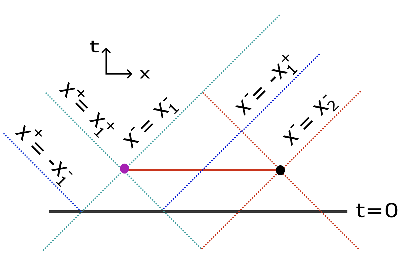
(a)

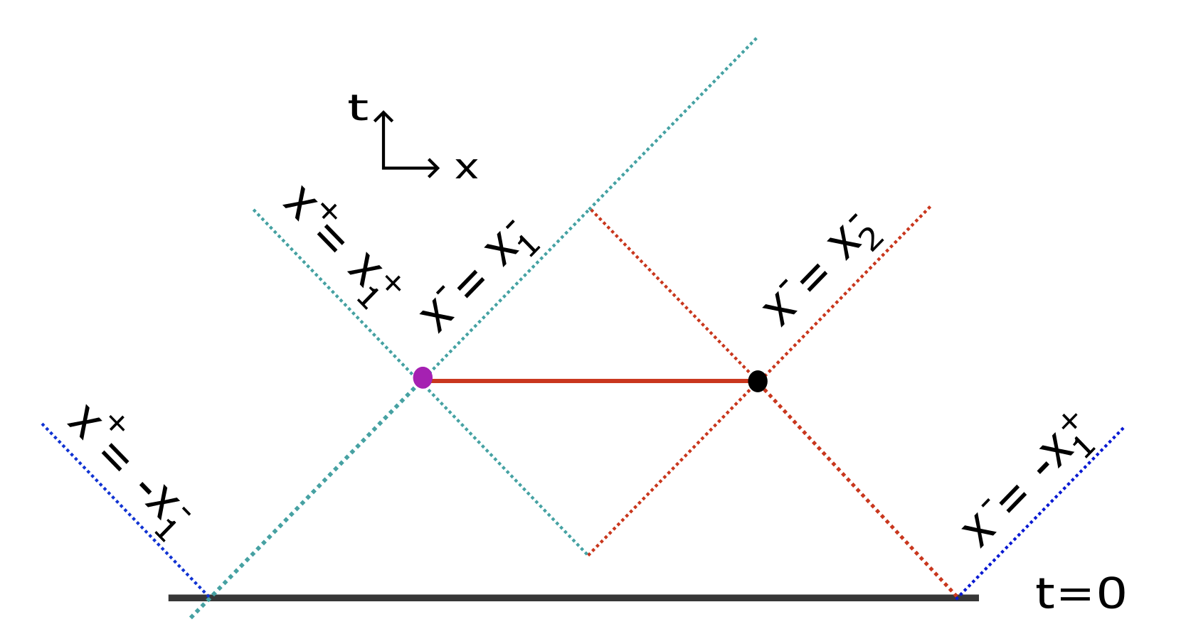
(b)

Figure 1: Figure to illustrate the limits of the ANE integrals. The interval of interest is shown in red with end-points marked in magenta and black. The QNEC is evaluated at the magenta point. The ANE operators are integrated along the cyan null directions. The null coordinates should be integrated for $t>0$. This leads to a lower bound of $x^{+}=-x_{1}^{-}$ and $x^{-}=-x_{1}^{+}$. (a) The case when $x_{2}^{-}<-x_{1}^{+}$. For the global quench this is when $t<\frac{l}{2}$. (b) The case when $x_{2}^{-}>-x_{1}^{+}$, corresponding to $t>\frac{l}{2}$ in the global quench.

From Fig. 1 it is easy to see that the $x^{-}$ coordinate, for the null cut at the first end-point of the interval, ranges from

$$x^{-}\in\left[\frac{l}{2}-t,\infty\right),$$ (27)

where the lower bound corresponds to the boundary at $t=0$.

Similarly, we can define $S(x^{+})$, which is needed to define the map $\bar{f}(x^{+})$ to a frame where the derivative of the entropy with respect to $x^{+}$ vanishes, by fixing the coordinates $x_{2}^{\pm}$ and $x_{1}^{-}$. In this case, we can again see from Fig. 1 that

$$x^{+}\in\left[-\frac{l}{2}-t,\infty\right).$$ (28)

We find that

$$\bar{f}(x_{2}^{+})\to\infty,\quad f(x_{2}^{-})\to\infty$$ (29)

Thus the ANE operator in the $f$-frame,

$$\int\braket{T(f)}df,$$ (30)

generates null deformations of the first end-point but doesn’t affect the second end-point. By transforming coordinates, we find

$$\braket{T(f)}= \ \left(\braket{T(x^{-})}+\frac{c}{24\pi}{\rm Sch}(f(x^{-}),x^{-})\right)f^{\prime}(x^{-})^{-2}$$

$$= \ \frac{1}{2\pi}\left(2\pi\braket{T(x^{-})}-\partial_{-}^{2}S(x^{-})+\frac{6}{c}(\partial_{-}S(x^{-}))^{2}\right)f^{\prime}(x^{-})^{-2},$$ (31)

$$= \ \frac{1}{2\pi}\mathcal{Q}_{-}(x^{-})f^{\prime}(x^{-})^{-1}$$ (32)

where we have used (25) to obtain the second equality.

To check whether our calculations and results satisfy the assumptions of the CF proof of QNEC, we need to check that the following is finite

$$\braket{\mathcal{\tilde{P}_{-}}}\coloneqq\frac{1}{2\pi}\int_{\frac{l}{2}-t}^{\infty}dx^{-}\mathcal{Q}_{-}(x^{-})f^{\prime}(x^{-})^{-1}.$$ (33)

A similar analysis applies for the anti-holomorphic part, for which we need to check finiteness of

$$\braket{\mathcal{\tilde{P}_{+}}}\coloneqq\frac{1}{2\pi}\int_{-\frac{l}{2}-t}^{\infty}dx^{+}\mathcal{Q}_{+}(x^{+})\bar{f}^{\prime}(x^{+})^{-1}.$$ (34)

Note that the derivatives that appear in the above integrals are non-negative, see (25). From this it is clear that QNEC violation for all $x^{\pm}$ would imply that the averaged null energy is negative, thus violating the averaged null energy condition (ANEC) in the $f$-frame.

We can explicitly compute the primary QNEC $\mathcal{Q}_{-}$ for arbitrary $x^{-}_{1}$ and fixed $x_{1}^{+},x_{2}^{\pm}$ with $t<\frac{l}{2}$. In this case the cross ratio $\eta$ remains approximately $0$ for the entire range of the integral and a theory independent analysis is therefore possible. Series expanding this expression in small $\epsilon$ we find that the integrand of $\braket{\mathcal{\tilde{P}}_{-}}$ is proportional to

$$\frac{c}{6}+\partial_{n}\tilde{\mathcal{F}}^{\prime}_{n}(0)|_{n=1},$$ (35)

with the proportionality constant being a non-negative function of $x^{-}$. The integral can be readily computed using the small $\epsilon$ expansion as

$$\braket{\mathcal{\tilde{P}_{-}}}=e^{\frac{-(l-4t)}{2\epsilon}}\frac{\epsilon^{3}}{\alpha\pi^{3}}\left(\frac{c}{6}+\partial_{n}\tilde{\mathcal{F}}^{\prime}_{n}(0)|_{n=1}\right)$$ (36)

The finiteness of this integral implies that the CF proof should apply and the primary QNEC $\mathcal{Q}_{-}\geq 0$ should be valid in this setup. A violation of the QNEC bound (22) implies that the ANEC is violated in the $f$-frame where the first null variation of the entanglement entropy vanishes.

When $t>\frac{l}{2}$, the range of the integral (33) crosses $x^{-}=0$. Similarly, the integral in the ANE (34) for the $+$ null direction crosses $x^{+}=0$ for both $t<\frac{l}{2}$ and $t>\frac{l}{2}$. Our analysis doesn’t shed light on the validity of the CF proof for $\mathcal{Q}_{\pm}$ in these cases. This is because the CFT description for the quench breaks down when $x^{\pm}$ are comparable to the cutoff $\epsilon$. The cutoff is related to the correlation length of the critical lattice system and the CFT description is valid at scales much larger than the correlation length Calabrese:2005in . Furthemore, the cross ratio $\eta$ as a function of $x^{+}$ varies from $0$ to $1$ along the range of the integral. As a function of $x^{-}$, when $t>\frac{l}{2}$, $\eta$ ranges from $2$ to $1$ along the range of the integral. The integral is then theory dependent, since we would need to know the function $\tilde{\mathcal{F}}_{n}$ explicitly for $\eta$ away from $0$ and $1$. It is thus not clear from our theory-independent CFT analysis if the CF proof in the $f$-frame and the primary QNEC apply to this setup in these cases.

We conclude this section by emphasising that the primary QNEC bounds (22) should be thought of as imposing constraints on the set of allowed boundary states such that these states satisfy the ANEC in a conformally transformed frame, where the first variation of the entanglement entropy, with respect to the $x^{-}$ direction, vanishes. Since a violation of QNEC implies a violation of causality under modular evolution Balakrishnan:2017bjg , we can also think of the bound (22) on the four point function as a modular causality restriction on the set of boundary states. Similar bounds on the three point correlators of the theory were found by demanding that the ANEC be satisfied Hofman:2008ar .

3 Local joining quench

In this section we consider the QNEC in a local joining quench Calabrese:2007mtj . Consider cutting a $1+1$ dimensional CFT at $x=0$ into two half lines $L$ and $R$. Prepare the half-line vacua on $L$ and $R$. The two halves are joined at time $t=0$. The state just before joining is simply the tensor product of the two half line vacua $\ket{0}_{L}\otimes\ket{0}_{R}$. The state after joining is evolved in time using the CFT Hamiltonian on the full line. Entanglement entropy can be calculated using a correlation function on the right half plane, similarly as described in the previous section.

The reduced density matrix of an interval can be computed using an Euclidean path integral on the plane with two slits on the imaginary time axis at $x=0$. One slit runs from Euclidean time $\tau=-\infty$ to $-\epsilon-it$ and the other runs from $\epsilon-it$ to $\infty$. The slits indicate that the two half lines are decoupled. As in the previous section, we also have a branch cut along the interval of interest. This plane with slits can be mapped to the half plane ${\rm Re}(z)>0$ via

$$z(w)=\frac{w}{\epsilon}+\sqrt{\frac{w^{2}}{\epsilon^{2}}+1}.$$ (37)

The Rènyi entropies and hence the entanglement entropy can be obtained using the correlator (4) on the half plane. The cross-ratio is now

$$\eta=\frac{(z_{1}+\bar{z}_{1})(z_{2}+\bar{z}_{2})}{(\bar{z}_{1}+z_{2})(z_{1}+\bar{z}_{2})},$$ (38)

and the entanglement entropy is

$$S_{A}=\frac{c}{6}\log\left[(z_{1}-z_{2})(\bar{z}_{1}-\bar{z}_{2})\eta\right]-\partial_{n}\tilde{\mathcal{F}}_{n}(\eta)|_{n=1}\ .$$ (39)

This can again be analytically continued to obtain expressions in terms of the lightcone coordinates. However, as noted for the global quench, we should first compute null derivatives and only then analytically continue to real time. Unlike the global quench, this subtlety in analytic continuation is important for the local quench because of the branch cut in the square root map between the $z$ and $w$ coordinates. The energy-momentum tensor is computed using the Schwarzian derivative of the above map and is

$$\braket{T_{\pm\pm}(x^{\pm})}=\frac{c}{16\pi}\frac{\epsilon^{2}}{({x^{\pm}}^{2}+\epsilon^{2})^{2}}.$$ (40)

Note that $\epsilon$ regulates the width of the energy-momentum tensor. In the $\epsilon\to 0$ limit this results in a $\delta$-function shockwave localized on the lightcone.

3.1 QNEC

One can evaluate the QNEC using the above expressions for entropy and energy-momentum tensor. There are various different choices for the entangling interval. For example, the interval can include or exclude the point $x=0$ where the two halves are joined. We take the end-points of the interval to be

$$x_{1}^{+}=t+l_{1},\quad x_{1}^{-}=t-l_{1},\qquad x_{2}^{+}=t+l_{2},\quad x_{2}^{-}=t-l_{2}.$$ (41)

Without loss of generality, we can assume that $l_{2}>l_{1}$. The cross-ratio $\eta$ varies depending on the choices for signs of the null coordinates. When $\eta$ is not close to zero or one, a theory-independent analysis is not possible. The two cases where a theory-independent analysis is possible are illustrated in Fig. 2.

If $x_{1,2}^{\pm}$ are all positive, i.e., when $t\pm l_{2}>0,t\pm l_{1}>0$, as indicated by the red interval in Fig. 2, we find that the conformal cross ratio $\eta\approx 1+\mathcal{O}(\epsilon^{4})$. In this case, we can evaluate the derivatives of entanglement entropy in a theory-independent manner. We get,

$$\mathcal{Q}_{1}^{-}= \ \frac{\epsilon^{2}}{4(t-l_{1})^{4}}\frac{2(t-l_{1})(t-l_{2})}{(t+l_{1})(t+l_{2})}\left(\frac{c}{6}-\partial_{n}\tilde{\mathcal{F}}_{n}^{\prime}(1)|_{n=1}\right),$$ (42)

$$\mathcal{Q}_{2}^{-}= \ \frac{\epsilon^{2}}{4(t-l_{2})^{4}}\frac{2(t-l_{1})(t-l_{2})}{(t+l_{1})(t+l_{2})}\left(\frac{c}{6}-\partial_{n}\tilde{\mathcal{F}}_{n}^{\prime}(1)|_{n=1}\right),$$ (43)

$$\mathcal{Q}_{1,2}^{+}= \ \frac{\epsilon^{2}(t+l_{2})}{2(t-l_{1})(t+l_{1})^{3}(t-l_{2})}\left(\frac{c}{6}-\partial_{n}\tilde{\mathcal{F}}_{n}^{\prime}(1)|_{n=1}\right)$$ (44)

Imposing $\mathcal{Q}_{1,2}^{\pm}\geq 0$ leads to the same bound on $\partial_{n}\tilde{\mathcal{F}}_{n}^{\prime}(1)|_{n=1}$ as the global quench (22). Note that the weak QNEC is always satisfied for this interval and is independent of $\tilde{\mathcal{F}}_{n}$ at leading order.

The other case where a theory-independent analysis is possible is when $x_{1}^{+}<0$ and the other lightcone coordinates are all positive (blue interval in Fig. 2). Note that since we have $l_{2}>l_{1}$, this case is only possible when $l_{1}<0$. The QNEC expressions for this case also involve $\left(\partial_{n}\tilde{\mathcal{F}}_{n}^{\prime}(1)|_{n=1}\right)^{2}$ at the leading order

$$\mathcal{Q}_{1}^{-}= \ \Bigg{(}\frac{c}{6}\frac{4(t-l_{1})^{2}(t-l_{2})(t+l_{1})}{l_{1}(l_{2}-l_{1})\epsilon^{2}}-\frac{4(t-l_{1})(t-l_{2})(t+l_{1})(l_{1}^{2}-3l_{1}l_{2}+3l_{1}t-l_{2}t)}{l_{1}(l_{2}-l_{1})(l_{2}+l_{1})\epsilon^{2}}\partial_{n}\tilde{\mathcal{F}}_{n}^{\prime}(1)|_{n=1}$$

$$\ -\frac{4(t+l_{1})^{2}(t-l_{2})^{2}}{(l_{2}+l_{1})^{2}\epsilon^{2}}\left(\partial_{n}\tilde{\mathcal{F}}_{n}^{\prime}(1)|_{n=1}\right)^{2}\Bigg{)}\frac{\epsilon^{2}}{4(t-l_{1})^{4}}.$$ (45)

It is easy to see that the above quadratic equation in $\partial_{n}\tilde{\mathcal{F}}_{n}^{\prime}(1)|_{n=1}$ is negative at $\partial_{n}\tilde{\mathcal{F}}_{n}^{\prime}(1)|_{n=1}\to\pm\infty$. Then, $\mathcal{Q}_{1}^{-}\geq 0$ requires that $\partial_{n}\tilde{\mathcal{F}}_{n}^{\prime}(1)|_{n=1}$ is bounded by the roots of $\mathcal{Q}^{-}_{1}=0$. We find that the larger root approaches its minimum value $\frac{c}{6}$ as $t\to-l_{1}$ and the smaller root approaches its maximum $-\frac{c}{6}$ as $t\to l_{2}$, leading to the following bounds

$$\frac{c}{3}\geq\frac{c}{6}-\partial_{n}\tilde{\mathcal{F}}_{n}^{\prime}(1)|_{n=1}\geq 0.$$ (46)

The lower bound above is the same as that obtained in the global quench (22), whereas the upper bound is a new result for the local quench. Similarly, we obtain

$$\mathcal{Q}_{1}^{+}= \ \frac{\epsilon^{2}}{4(t+l_{1})^{4}}\Bigg{(}\frac{4\partial_{n}\tilde{\mathcal{F}}_{n}^{\prime}(1)|_{n=1}(l_{1}-l_{2})(l_{1}+t)^{3}(l_{2}-t)\left(l_{1}^{2}-3l_{1}l_{2}+3l_{1}t-l_{2}t\right)}{l_{1}\epsilon^{2}(l_{1}+l_{2})^{3}(l_{1}-t)}$$ (47)

$$\ -\frac{4\left(\partial_{n}\tilde{\mathcal{F}}_{n}^{\prime}(1)|_{n=1}\right)^{2}(l_{1}-l_{2})^{2}(l_{1}+t)^{4}(l_{2}-t)^{2}}{\epsilon^{2}(l_{1}+l_{2})^{4}(l_{1}-t)^{2}}+\frac{2c(l_{1}-l_{2})(l_{1}+t)^{3}(l_{2}-t)}{3l_{1}\epsilon^{2}(l_{1}+l_{2})^{2}}\Bigg{)},$$

$$\mathcal{Q}_{2}^{-}= \ \frac{\epsilon^{2}}{4(t-l_{2})^{4}}\Bigg{(}\frac{8cl_{1}(l_{1}+t)(l_{2}-t)^{3}}{3\epsilon^{2}(l_{1}-l_{2})(l_{1}+l_{2})^{2}}-\frac{16l_{1}^{2}\left(\partial_{n}\tilde{\mathcal{F}}_{n}^{\prime}(1)|_{n=1}\right)^{2}(l_{1}+t)^{2}(l_{2}-t)^{4}}{\epsilon^{2}(l_{1}+l_{2})^{4}(l_{1}-t)^{2}}$$

$$\ +\frac{16l_{1}\partial_{n}\tilde{\mathcal{F}}_{n}^{\prime}(1)|_{n=1}(l_{1}+t)(l_{2}-t)^{3}\left(l_{1}^{2}-3l_{1}l_{2}+3l_{1}t-l_{2}t\right)}{\epsilon^{2}(l_{1}-l_{2})(l_{1}+l_{2})^{3}(l_{1}-t)}\Bigg{)},$$ (48)

$$\mathcal{Q}_{2}^{+}= \ \frac{4}{\epsilon^{2}}\Bigg{(}\frac{2c(l_{1}-l_{2})(l_{1}+t)^{3}(l_{2}-t)}{3l_{1}\epsilon^{2}(l_{1}+l_{2})^{2}}-\frac{4\left(\partial_{n}\tilde{\mathcal{F}}_{n}^{\prime}(1)|_{n=1}\right)^{2}(l_{1}-l_{2})^{2}(l_{1}+t)^{4}(l_{2}-t)^{2}}{\epsilon^{2}(l_{1}+l_{2})^{4}(l_{1}-t)^{2}}$$

$$\ +\frac{4\partial_{n}\tilde{\mathcal{F}}_{n}^{\prime}(1)|_{n=1}(l_{1}-l_{2})(l_{1}+t)^{3}(l_{2}-t)\left(l_{1}^{2}-3l_{1}l_{2}+3l_{1}t-l_{2}t\right)}{l_{1}\epsilon^{2}(l_{1}+l_{2})^{3}(l_{1}-t)}\Bigg{)}.$$ (49)

We analyse the QNECs above in the same way as $\mathcal{Q}_{1}^{-}$ (45) and obtain the same bounds (46).

We also calculate the weak QNEC in this case. Unlike the global quench, we find that even the weak QNEC imposes bounds on $\partial_{n}\tilde{\mathcal{F}}_{n}^{\prime}(1)|_{n=1}$. When $x_{1,2}^{\pm}$ are all positive, all the weak QNEC inequalities evaluate to the same form and are trivially satisfied,

$$Q_{1,2}^{\pm}= \ \frac{c}{6(l_{1}-l_{2})^{2}}>0.$$ (50)

For the other interval where a theory-independent analysis is possible, with $x_{1}^{+}<0,x_{1}^{-}>0,x_{2}^{\pm}>0,$ we get the following,

$$Q_{1}^{-}= \ \frac{c}{24}\left(\frac{1}{l_{1}^{2}}+\frac{4}{(l_{1}-l_{2})^{2}}-\frac{4}{(l_{1}-t)^{2}}\right)+\frac{2(l_{1}+t)(l_{2}-t)}{(l_{1}+l_{2})(l_{1}-t)^{3}}\partial_{n}\tilde{\mathcal{F}}_{n}^{\prime}(1)|_{n=1}$$

$$Q_{1}^{+}= \ \frac{c}{24}\left(\frac{1}{l_{1}^{2}}-\frac{4}{(l_{1}+l_{2})^{2}}+\frac{4}{(l_{1}+t)^{2}}\right)+\frac{2(l_{1}-l_{2})(l_{2}-t)}{(l_{1}+l_{2})^{3}(l_{1}-t)}\partial_{n}\tilde{\mathcal{F}}_{n}^{\prime}(1)|_{n=1}$$ (51)

$$Q_{2}^{-}= \ \frac{1}{6(l_{1}+l_{2})^{3}}\left(\frac{c(l_{1}+l_{2})\left(l_{1}^{4}-2l_{1}^{2}l_{2}^{2}+4l_{1}l_{2}(l_{2}-t)^{2}+l_{2}^{4}\right)}{(l_{1}-l_{2})^{2}(l_{2}-t)^{2}}-\frac{24l_{1}(l_{1}+t)}{l_{1}-t}\partial_{n}\tilde{\mathcal{F}}_{n}^{\prime}(1)|_{n=1}\right)$$

$$Q_{2}^{+}= \ \frac{c}{6(l_{2}+t)^{2}}$$

The solution of, e.g., $Q_{1}^{-}=0$ for $\partial_{n}\tilde{\mathcal{F}}_{n}^{\prime}(1)|_{n=1}$ is dimensionless. If we choose the dimensionless variables to be say $l_{2}/l_{1}$ and $t/l_{1}$, we further notice that the range of these coordinates is finite due to the choice of our entangling region. By searching numerically over this compact range, we find that the strongest bounds from these inequalities in fact approach the same bounds (46) as those from the primary QNEC. This happens for intervals where $t,l_{2}\to-l_{1}$, i.e., intervals where both end-points are close to the two shock-waves, but $x_{1}^{+}<0$ and $x_{2}^{-}>0$. As expected, the weak QNEC bounds are always weaker than the bounds from the primary QNEC.

The weak QNEC bounds are only obtained for the blue region in Fig. 2. This region crosses the shock-wave, and the red region that trivially satisfies the weak QNEC does not cross any shocks.

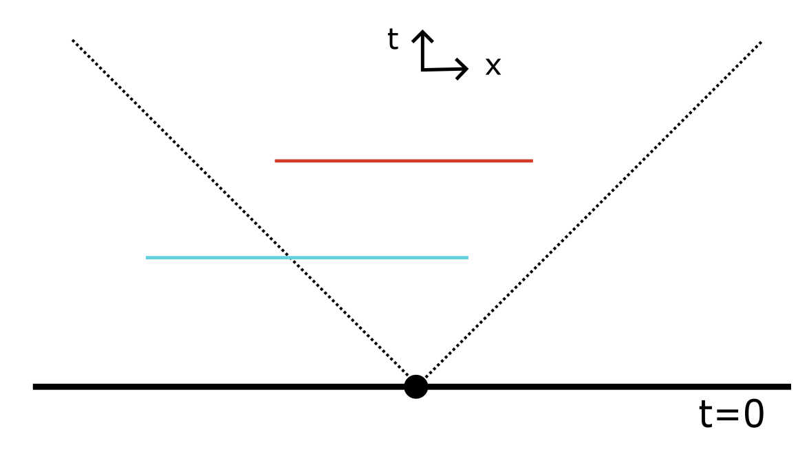
Figure 2: A plot to illustrate the entangling regions where a theory-independent primary QNEC can be calculated. The black circle indicates the point $x=0$ where the two half lines are joined. The dashed lines are the (regulated) shockwaves propagating along the null directions. Note that the red interval trivially satisfies the weak QNEC, whereas the blue interval leads to non-trivial bounds from the weak QNEC.

3.2 Averaged null energy

We expect that the post local quench state has finite relative entropy with respect to the CFT vacuum since it is in the identity sector – the fusion of two identities can only produce identity and descendants Stephan:2011kcw . It is easy to see that the ANE for the weak QNEC is finite whenever the integral doesn’t cross $x^{\pm}=0$. Thus the CF proof should hold for $Q_{-}$ in the case with $x_{1}^{-}<0,x_{1}^{+}>0,x_{2}^{\pm}>0.$

To understand if the primary QNEC holds, we must perform a similar analysis as that performed in Sec. 2.3 and verify if the ANE is finite. We need to evaluate the following integrals (see (33), (34))

$$\braket{\mathcal{\tilde{P}_{-}}} \coloneqq\frac{1}{2\pi}\int_{-l_{1}-t}^{\infty}dx^{-}\mathcal{Q}_{-}(x^{-})f^{\prime}(x^{-})^{-1}$$ (52)

$$\braket{\mathcal{\tilde{P}_{+}}} \coloneqq\frac{1}{2\pi}\int_{l_{1}-t}^{\infty}dx^{+}\mathcal{Q}_{+}(x^{+})\bar{f}^{\prime}(x^{+})^{-1}.$$ (53)

In the cases where a theory independent analysis of QNEC is possible, we find that a theory-independent analysis of the ANE is not possible. Either the cross-ratio is not near 0 or 1, or the range of the integral crosses $x^{\pm}=0$ where the CFT description breaks down. Therefore, in the local quench we are unable to evaluate the ANEs relevant to the primary QNEC and check for their finiteness without invoking an explicit theory. This implies that we cannot establish that the primary QNEC must hold for this quench. It would be interesting to study QNEC and the ANE in this quench for some explicit theories.

4 Discussion

CFT

The quantum null energy condition has been proven in a variety of contexts Bousso:2015wca ; Malik:2019dpg ; Koeller:2015qmn ; Balakrishnan:2017bjg . QNEC was proven in general Poincaré invariant quantum field theories for null cuts, in states with finite averaged null energy (ANE) and finite relative entropy with respect to the vacuum state by Ceyhan and Faulkner Ceyhan:2018zfg . Out of these two restrictions, finite relative entropy is essential for the QNEC to be well defined.

In order to understand our results in the context of the Ceyhan-Faulkner proof, we have tried to examine if the setups studied here satisfy the two assumptions made in the proof. We have argued for the finiteness of relative entropies of the out-of-equilibrium states we study here, and have computed the ANE whenever it is well defined in a theory-independent way.

For the global quench we find that the primary QNEC imposes bounds on the theory dependent function $\partial_{n}\tilde{\mathcal{F}}_{n}$, and hence on the two point functions of twist fields on the UHP. In the case where a theory-independent analysis is possible (36), we find that whenever the primary QNEC bounds are satisfied then $0<\braket{\tilde{\mathcal{P}}}<\infty$, and a violation of these bounds implies a violation of the ANEC in a conformally transformed frame. The ANEC has been proven for general quantum field theories Klinkhammer:1991ki ; Kelly:2014mra ; Faulkner:2016mzt ; Hartman:2016lgu ; Kravchuk:2018htv , although the presence of boundaries needs some care Fewster:2006uf . Our bounds can be thought of as additional restrictions on the allowed boundary states, arising from the ANEC and also from causality in modular time Balakrishnan:2017bjg .

As far as we are aware the function $\tilde{\mathcal{F}}_{n}$ has not been calculated explicitly for non-integer $n$ in any theory. For example, the function $\mathcal{F}_{n}$ which appears in the four point correlator on the plane has been calculated for integer $n$ for the Luttinger liquid Calabrese:2009ez , however the analytic continuation to non-integer $n$ is not straightforward. Our bounds from QNEC place restrictions on the analytic continuations of related functions $\tilde{\mathcal{F}}_{n}$ that are allowed for non-integer $n\gtrsim 1$. It would be interesting to explicitly compute the analytically continued $\tilde{\mathcal{F}}$ in some theories in consistency with the bounds we have derived.

For the local quench, we again find bounds on $\partial_{n}\tilde{\mathcal{F}}_{n}$ from primary QNEC. Furthermore, in this setup, the weak QNEC also imposes bounds on $\partial_{n}\tilde{\mathcal{F}}_{n}$, that are weaker than the primary QNEC but approach those bounds in a certain limit. We cannot calculate the ANE for the primary QNEC in a theory independent manner for any interval in the local quench, and therefore cannot comment on the validity of the CF proof to this setup.

Holography

We have performed our calculations of QNEC entirely within CFT, without assuming an Einstein gravity dual. Our results will also hold in the large central charge and sparse spectrum limit, i.e., when an Einstein dual exists for the CFT. The holographic proof of QNEC Koeller:2015qmn is applicable to the quenches considered here. Therefore, we should also understand the QNEC violations we find in the context of the holographic proof.

The bulk dual of the global quench, in the UHP coordinates, is simply vacuum AdS₃ with an end-of-the-world brane corresponding to the boundary at $t=0$. The bulk dual for the post local quench state discussed here is a locally AdS₃ Bañados geometry Banados:1998gg with an end of the world brane. In the local quench the regime where we find non-trivial bounds corresponds to bulk geodesics that intersect the end of the world brane. This can be deduced from the entanglement entropy, which is different from the entropy for the connected geodesic in a Bañados geometry. The holographic QNEC follows from bulk entanglement wedge nesting. As discussed in a footnote in Wall:2012uf , consistency theorems (such as nesting) for extremal surfaces that compute holographic entanglement entropy can fail in spacetimes with boundaries at a finite distance. For example, violations of strong sub-additivity of holographic entanglement entropy have been found in cases where the bulk duals are at a finite radial cutoff Sanches:2016sxy ; Grado-White:2020wlb . Thus, our results do not contradict the holographic proof of QNEC. We also note that Banerjee:2024wtl do not find any violations of QNEC for $T\bar{T}$-deformation of 2d CFTs, implying that the presence of finite boundaries does not necessarily imply violations of QNEC. It wil be interesting to relate the recent discussion of entanglement wedge nesting in the presence of end of the world branes in Saraswat:2025gxp with our results for QNEC.

Future directions

In this paper we have considered the simplest local joining quench where two half-line vacua are connected suddenly. More general setups where the two half-lines have different temperatures have been studied Bernard:2016nci . Interesting steady-state formation has been observed in such setups, which have also been studied holographically in Erdmenger:2017gdk . It would be interesting to examine QNEC in these setups.

A Rènyi generalization of the QNEC Lashkari:2018nsl , which uses the sandwiched Rènyi divergences, has been proven for free field theories Moosa:2020jwt ; Roy:2022yzm . However, it is still unclear if the Rènyi QNEC is valid more generally. The quenches studied in this work are a natural place to explicitly compute and test the Rènyi QNEC in non-trivial out-of-equilibrium states using both holography and purely CFT techniques.

Furthermore, using the map between the Temperley-Lieb and Virasoro algebras Koo:1993wz it might be possible to understand the implications of QNEC directly on spin chains. This can likely shed some further light on the QNEC violations we find in this paper.

Acknowledgements

We would like to thank Thomas Faulkner for valuable discussions and for pointing us to the correct ANE operator that should be checked for finiteness. We would also like to thank Aron Wall for helpful correspondence. We are also grateful to Adwait Gaikwad, Sam van Leuven, Ayan Mukhopadhyay, and Ronak Soni for helpful discussions. The research of PR is supported by an NRF Freestanding Postdoctoral Fellowship. PR would like to thank Chennai Mathematical Institute for their generous hospitality during the initial stages of this work.

References

- (1) T. Faulkner, T. Hartman, M. Headrick, M. Rangamani and B. Swingle, Snowmass white paper: Quantum information in quantum field theory and quantum gravity, in Snowmass 2021, 3, 2022 [2203.07117].
- (2) A.C. Wall, Lower Bound on the Energy Density in Classical and Quantum Field Theories, Phys. Rev. Lett. 118 (2017) 151601 [1701.03196].
- (3) R. Landauer, Irreversibility and heat generation in the computing process, IBM Journal of Research and Development 5 (1961) 183.
- (4) R. Landauer, Information is physical, Physics Today 44 (1991) 23 [https://pubs.aip.org/physicstoday/article-pdf/44/5/23/8304036/23_1_online.pdf].
- (5) D. Reeb and M.M. Wolf, An improved landauer principle with finite-size corrections, New Journal of Physics 16 (2014) 103011.
- (6) R. Bousso, Z. Fisher, S. Leichenauer and A.C. Wall, Quantum focusing conjecture, Phys. Rev. D 93 (2016) 064044 [1506.02669].
- (7) R. Bousso, Z. Fisher, J. Koeller, S. Leichenauer and A.C. Wall, Proof of the Quantum Null Energy Condition, Phys. Rev. D 93 (2016) 024017 [1509.02542].
- (8) T.A. Malik and R. Lopez-Mobilia, Proof of the quantum null energy condition for free fermionic field theories, Phys. Rev. D 101 (2020) 066028 [1910.07594].
- (9) J. Koeller and S. Leichenauer, Holographic Proof of the Quantum Null Energy Condition, Phys. Rev. D 94 (2016) 024026 [1512.06109].
- (10) S. Balakrishnan, T. Faulkner, Z.U. Khandker and H. Wang, A General Proof of the Quantum Null Energy Condition, JHEP 09 (2019) 020 [1706.09432].
- (11) F. Ceyhan and T. Faulkner, Recovering the QNEC from the ANEC, Commun. Math. Phys. 377 (2020) 999 [1812.04683].
- (12) S. Hollands and R. Longo, A New Proof of the QNEC, 2503.04651.
- (13) T. Kibe, A. Mukhopadhyay and P. Roy, Quantum Thermodynamics of Holographic Quenches and Bounds on the Growth of Entanglement from the Quantum Null Energy Condition, Phys. Rev. Lett. 128 (2022) 191602 [2109.09914].
- (14) A. Banerjee, T. Kibe, N. Mittal, A. Mukhopadhyay and P. Roy, Erasure Tolerant Quantum Memory and the Quantum Null Energy Condition in Holographic Systems, Phys. Rev. Lett. 129 (2022) 191601 [2202.00022].
- (15) T. Kibe, A. Mukhopadhyay and P. Roy, Generalized Clausius inequalities and entanglement production in holographic two-dimensional CFTs, 2412.13256.
- (16) S. Deffner and E. Lutz, Generalized clausius inequality for nonequilibrium quantum processes, Phys. Rev. Lett. 105 (2010) 170402.
- (17) A.C. Wall, Testing the Generalized Second Law in 1+1 dimensional Conformal Vacua: An Argument for the Causal Horizon, Phys. Rev. D 85 (2012) 024015 [1105.3520].
- (18) P. Calabrese and J.L. Cardy, Evolution of entanglement entropy in one-dimensional systems, J. Stat. Mech. 0504 (2005) P04010 [cond-mat/0503393].
- (19) P. Calabrese and J. Cardy, Entanglement and correlation functions following a local quench: a conformal field theory approach, J. Stat. Mech. 0710 (2007) P10004 [0708.3750].
- (20) P. Calabrese and J.L. Cardy, Entanglement entropy and quantum field theory, J. Stat. Mech. 0406 (2004) P06002 [hep-th/0405152].
- (21) P. Calabrese and J. Cardy, Entanglement entropy and conformal field theory, J. Phys. A 42 (2009) 504005 [0905.4013].
- (22) M. Mezei and J. Virrueta, The Quantum Null Energy Condition and Entanglement Entropy in Quenches, 1909.00919.
- (23) D.M. Hofman and J. Maldacena, Conformal collider physics: Energy and charge correlations, JHEP 05 (2008) 012 [0803.1467].
- (24) J.-M. Stéphan and J. Dubail, Local quantum quenches in critical one-dimensional systems: entanglement, the Loschmidt echo, and light-cone effects, J. Stat. Mech. 2011 (2011) P08019 [1105.4846].
- (25) G. Klinkhammer, Averaged energy conditions for free scalar fields in flat space-times, Phys. Rev. D 43 (1991) 2542.
- (26) W.R. Kelly and A.C. Wall, Holographic proof of the averaged null energy condition, Phys. Rev. D 90 (2014) 106003 [1408.3566].
- (27) T. Faulkner, R.G. Leigh, O. Parrikar and H. Wang, Modular Hamiltonians for Deformed Half-Spaces and the Averaged Null Energy Condition, JHEP 09 (2016) 038 [1605.08072].
- (28) T. Hartman, S. Kundu and A. Tajdini, Averaged Null Energy Condition from Causality, JHEP 07 (2017) 066 [1610.05308].
- (29) P. Kravchuk and D. Simmons-Duffin, Light-ray operators in conformal field theory, JHEP 11 (2018) 102 [1805.00098].
- (30) C.J. Fewster, K.D. Olum and M.J. Pfenning, Averaged null energy condition in spacetimes with boundaries, Phys. Rev. D 75 (2007) 025007 [gr-qc/0609007].
- (31) P. Calabrese, J. Cardy and E. Tonni, Entanglement entropy of two disjoint intervals in conformal field theory, J. Stat. Mech. 0911 (2009) P11001 [0905.2069].
- (32) M. Banados, Three-dimensional quantum geometry and black holes, AIP Conf. Proc. 484 (1999) 147 [hep-th/9901148].
- (33) A.C. Wall, Maximin Surfaces, and the Strong Subadditivity of the Covariant Holographic Entanglement Entropy, Class. Quant. Grav. 31 (2014) 225007 [1211.3494].
- (34) F. Sanches and S.J. Weinberg, Holographic entanglement entropy conjecture for general spacetimes, Phys. Rev. D 94 (2016) 084034 [1603.05250].
- (35) B. Grado-White, D. Marolf and S.J. Weinberg, Radial Cutoffs and Holographic Entanglement, JHEP 01 (2021) 009 [2008.07022].
- (36) A. Banerjee and P. Roy, Bounds on deformation from entanglement, JHEP 10 (2024) 064 [2404.16946].
- (37) K. Saraswat, Constraints from Entanglement Wedge Nesting for Holography at a Finite Cutoff, 2501.15024.
- (38) D. Bernard and B. Doyon, Conformal field theory out of equilibrium: a review, J. Stat. Mech. 1606 (2016) 064005 [1603.07765].
- (39) J. Erdmenger, D. Fernandez, M. Flory, E. Megias, A.-K. Straub and P. Witkowski, Time evolution of entanglement for holographic steady state formation, JHEP 10 (2017) 034 [1705.04696].
- (40) N. Lashkari, Constraining Quantum Fields using Modular Theory, JHEP 01 (2019) 059 [1810.09306].
- (41) M. Moosa, P. Rath and V.P. Su, A Rényi quantum null energy condition: proof for free field theories, JHEP 01 (2021) 064 [2007.15025].
- (42) P. Roy, Proof of the Rényi quantum null energy condition for free fermions, Phys. Rev. D 108 (2023) 045010 [2212.02331].
- (43) W.M. Koo and H. Saleur, Representations of the Virasoro algebra from lattice models, Nucl. Phys. B 426 (1994) 459 [hep-th/9312156].