Evaluating the faithfulness of PDF uncertainties in the presence of inconsistent data

Abstract

We critically assess the robustness of uncertainties on parton distribution functions (PDFs) determined using neural networks from global sets of experimental data collected from multiple experiments. We view the determination of PDFs as an inverse problem, and we study the way the neural network model tackles it when inconsistencies between input datasets are present. We use a closure test approach, in which the regression model is applied to artificial data produced from a known underlying truth, to which the output of the model can be compared and its accuracy can be assessed in a statistically reliable way. We explore various phenomenologically relevant scenarios in which inconsistencies arise due to incorrect estimation of correlated systematic uncertainties. We show that the neural network generally corrects for the inconsistency except in cases of extreme uncertainty underestimation. When the inconsistency is not corrected, we propose and validate a procedure to detect inconsistencies.

1 Introduction

The accurate estimate of uncertainties on Parton Distribution Functions (PDFs) is necessary for precision phenomenology, see Amoroso:2022eow ; Ubiali:2024pyg for recent reviews. Because PDFs are extracted by comparing to experimental data theory predictions obtained using them, their determination falls into the general category of inverse problems, i.e. problems in which a model is inferred starting from a finite set of observations, which are both noisy and sometimes incompatible with one another. Machine Learning is currently widely used in this context see Refs. Guest:2018yhq ; Albertsson:2018maf ; Plehn:2022ftl for comprehensive reviews.

The NNPDF collaboration uses machine learning techniques for the determination of PDFs and their uncertainties, by combining a parametrization of PDFs through a feed–forward neural network with a Monte Carlo importance sampling procedure to propagate the data uncertainty in the space of PDFs. The faithfulness of a regression model’s uncertainties can be assessed by means of a closure test. In the context of PDFs, this has been first done by NNPDF in Ref. Ball:2014uwa , following a suggestion in Ref. demortier and previous studies in Ref. Watt:2012tq . A detailed theoretical discussion of the statistical underpinnings of the closure testing methodology is given in Ref. DelDebbio:2021whr . Similar studies have been recently also performed in the context of PDF fitting methodologies based on a fixed polynomial parametrization and Hessian approach for uncertainty propagation in parameter space Harland-Lang:2024kvt . The idea of closure tests is to apply the regression model to artificial data generated from a known underlying truth. In this case the underlying law of Nature (i.e. the PDFs) is known. The model is however run without exploiting this knowledge, as would be the case in a realistic situation. By performing the procedure repeatedly it is possible to test whether the distribution of results about the underlying truth faithfully reproduces their nominal uncertainties (including their correlation), thereby validating the accuracy of the model uncertainty estimate.

Closure tests so far have been performed on a set of consistent artificial data, meaning that the theory predictions and the uncertainties that are used in the generation of the data are the same ones that the model then uses for regression. However, in a realistic case both theory prediction and uncertainty could be inconsistent. The former case corresponds to a situation in which the theory used in regression is the Standard Model (SM), while the data actually contain physics beyond the SM. This situation has been studied in Refs. Hammou:2023heg ; Costantini:2024xae ; Hammou:2024xuj , in which closure tests were used to investigate whether in such a situation possible new physics would be detected. The latter case corresponds to a situation in which the actual statistical distribution of data differs from the covariance matrix that is supposed to describe them, for instance because some sources of systematic uncertainty have not been correctly estimated.

In this work we explore what happens when inconsistencies of experimental origin are present in the training dataset. The use of closure tests in a context in which an inconsistency is injected in the data in a controlled way allows testing the behavior of the model in a situation that may well happen in real-world situations. As by-products of our investigation, we consolidate and improve the closure test methodology, and we validate a procedure aimed at singling out inconsistent datasets, improving over a previously proposed procedure NNPDF:2021njg .

The paper is organised as follows. In Sect. 2 we summarise our methodology: first, we briefly review the NNPDF methodology for PDF determination, then we summarise the principles of closure testing it in the approach of Refs. Ball:2014uwa ; DelDebbio:2021whr , and finally we discuss how inconsistencies can be introduced in the closure testing methodology. In Sect. 3 we present results in different representative inconsistency scenarios that differ both in the degree of inconsistency introduced, in the relative size of the inconsistent dataset compared to the global dataset, and in the presence or absence of other consistent datasets similar in nature to the inconsistent one, specifically assessing the extent to which the model manages to correct for the inconsistency. In Sect. 4 we construct and validate a diagnostic tool that can be used to detect situations in which the inconsistency is not corrected, improving upon a methodology previously proposed and adopted by the NNPDF collaboration in Ref. NNPDF:2021njg .

2 Closure tests and inconsistent data

We discuss here the idea of closure testing the impact of inconsistent data. We start by presenting in Sect. 2.1 a brief review of the way PDFs and their uncertainties are obtained within the NNPDF approach, in Sect. 2.2 we then briefly summarise the way closure tests can be used to test it, specifically by defining suitable statistical estimators, and finally in Sect. 2.3 we present the way the effect of data inconsistencies can be studied through closure tests.

2.1 The NNPDF approach to PDF determination

The NNPDF approach uses the Monte Carlo (MC) replica method for the propagation of experimental and model uncertainties onto the PDF functional space. The MC replica method consists in determining a set of fit outcomes to approximate the posterior probability distribution of the PDF model given a set of experimental input data. The input data are in turn represented as a MC sample of $N_{\rm rep}$ pseudodata replicas whose distribution (typically a multivariate normal) reproduces the covariance matrix of the experimental data. The fit outcomes are determined by comparing to the data replicas predictions that depend on PDFs via a forward map ${\cal G}$. The MC replica method shares similarities with the parametric bootstrap Hall1992TheBA approach in statistical literature, see Ref. Costantini:2024wby for an analytical expression for the posterior distribution of the model derived from this method.

Following the notation of Ref. DelDebbio:2021whr , if we assume that the observational noise of the experimental data can be approximated as a vector drawn from a multivariate normal distribution with a given covariance matrix $C$, the central experimental values, $y_{0}$, are given by

$$y_{0} =f+\eta,$$ (1)

where $f\in\mathbb{R}^{N_{\rm data}}$ is the vector of true, thus unknown, observable values and $\eta$ is the observational noise drawn from a Gaussian $\mathcal{N}(0,C)$ centred on zero with covariance matrix $C$. This covariance matrix contains both statistical uncertainties (mostly but not always uncorrelated) and systematic uncertainties (mostly correlated). Note that some systematic uncertainties are actually of theoretical origin, in that they affect the relation of the quantity that is actually measured to the experimental (pseudo)-observable for which theory predictions are obtained. Examples are electroweak corrections, sometimes already subtracted by experimental collaborations in order to obtain their published data, or nuclear corrections that relate nuclear to proton structure functions. The vector $\eta$ accordingly induces correlations among data points that reflect those contained in the $C$ matrix.

In the NNPDF approach, pseudodata replicas of the data are generated by augmenting $y_{0}$ with noise $\epsilon^{(k)}$

$$\mu^{(k)} =y_{0}+\epsilon^{(k)}=f+\eta+\epsilon^{(k)},\quad k=1,...,N_{\rm rep},$$ (2)

where $k$ is the replica index and $N_{\rm rep}$ is the number of pseudodata replicas. Each instance of the noise $\epsilon^{(k)}$ is drawn independently from the same multi-Gaussian distribution $\mathcal{N}(0,C)$, which the observational noise is drawn from. This implies that the covariance of any two data points over the replica sample in the limit of large $N_{\rm rep}$ tends to the corresponding $C$ matrix element.

An optimal model replica is then determined for each data replica by minimizing a loss function computed on a training subset of data and stopping the training conditionally on the loss computed on the remaining (validation) data subset. Namely, by determining for each replica $k$ the values $u_{*,k}$ of the parameters $u$ of a model $w(u)$ of the PDFs $w$ such that

$$u_{*,k} =\operatorname*{argmin}_{u_{k}}\left[\chi_{\rm val}^{2(k)}|\operatorname*{argmin}_{u_{k}}\chi_{\rm tr}^{2(k)}\right],\quad k=1,...,N_{\rm rep},$$ (3)

where $\chi_{\rm tr}^{2(k)}$ and $\chi_{\rm val}^{2(k)}$ are the training and validation loss, and the notation means that the minimum validation loss is picked conditional to the minimisation of the training loss.

The loss function is chosen as a maximum likelihood estimator, namely

$$\chi^{2(k)}(C) =\frac{1}{N_{\rm data}}\left({\cal G}(w(u_{k}))-\mu^{(k)}\right)^{T}C^{-1}\left({\cal G}(w(u_{k}))-\mu^{(k)}\right),$$ (4)

where ${\cal G}(w)$ is the forward map, that maps the PDF $w$ to the measured observable to which the pseudodata replica $\mu^{(k)}$ values Eq. (2) refer to. The forward map is constructed by evolving the PDF to the appropriate scale and folding them with partonic cross-sections to get observables. The training and validation losses $\chi_{\rm tr}^{2(k)}$ and $\chi_{\rm val}^{2(k)}$ are respectively defined by only including in Eq. (4) the data in the respective subset. The final outcome of the procedure is thus a set of PDF model replicas $w(u_{*,k})$ from which the predicted PDFs can be determined as

$$w^{\rm pred}=\mathbb{E}_{\epsilon}\left[w(u_{*,k})\right],$$ (5)

where here and henceforth $\mathbb{E}_{\epsilon}$ denotes the average over the replica sample. Similarly, one can determine the prediction for any set of PDF-dependent physical observables as

$${\cal G}^{\rm pred}=\mathbb{E}_{\epsilon}\left[{\cal G}(w(u_{*,k}))\right].$$ (6)

Uncertainties on the predictions and their correlations can be further determined from higher moments of the distribution $w(u_{*,k})$ of PDF replicas. In particular, the predicted PDF uncertainties are given by the diagonal elements of the covariance matrix

$$\left(C_{\rm PDF}\right)_{ij}=\frac{N_{\rm reps}}{N_{\rm reps}-1}\mathbb{E}_{\epsilon}\left[\left({\cal G}(u_{*,k})_{i}-\mathbb{E}_{\epsilon}{\cal G}(u_{*,k})_{i}\right)\left({\cal G}(u_{*,k})_{j}-\mathbb{E}_{\epsilon}{\cal G}(u_{*,k})_{j}\right)\right]$$ (7)

whose off-diagonal elements provide the PDF-induced correlations.

The model adopted by NNPDF is a feed-forward neural network, whose weights and thresholds are the parameters $u$. The architecture, initialisation and activation function of the neural network are determined through a hyperoptimisation procedure. The loss minimisation is performed using a gradient descent algorithm. The algorithm and its parameters are also part of the hyperoptimisation.

In order to compute quantities of physical interest, it is necessary to invert the covariance matrix $C_{\rm PDF}$, which has dimension $N_{\rm data}\times N_{\rm data}$, and is computed from the underlying PDFs. The full dataset contains several thousand datapoints. On the other hand, it is known Carrazza:2015aoa ; PDF4LHCWorkingGroup:2022cjn that for current PDF sets an accurate representation of the full PDF covariance matrix can be obtained by means of a Hessian representation with a much smaller number of eigenvectors, between $50$ and $100$ Carrazza:2015hva ; Carrazza:2015aoa ; Carrazza:2016htc . This means that the full $C_{\rm PDF}$ matrix is necessarily poorly conditioned. Namely, the condition number, defined as

$$\kappa(C_{\rm PDF})=\frac{|\lambda_{\rm max}(C_{\rm PDF})|}{|\lambda_{\rm min}(C_{\rm PDF})|},$$ (8)

where $\lambda_{\rm max}$ and $\lambda_{\rm min}$ are respectively the largest and smallest eigenvalue of the covariance matrix $C_{\rm PDF})$, is very large. Furthermore, even the restriction of $C_{\rm PDF}$ to individual datasets, with a number of datapoints of order of a hundred, or even ten, is generally poorly conditioned, because individual datasets are typically correlated only to a small number of PDFs or PDF combinations in a limited kinematic region (see e.g. Forte:2010dt ).

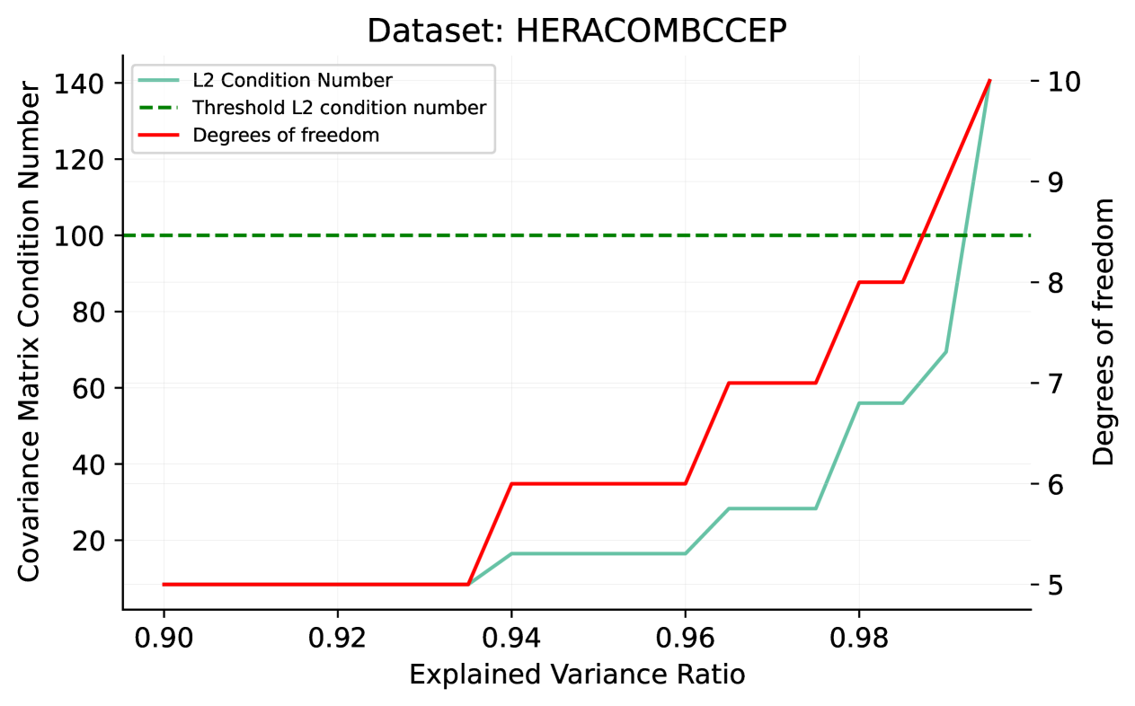
Figure 1: Condition number for the HERA I+II inclusive CC dataset (see Table 1 ) as a function of the explained variance ratio, namely the ratio of the traces of the regularised to full covariance matrix.

This problem can be addressed by only retaining the contribution to the covariance matrix of the eigenvectors with largest eigenvalues, i.e., to regularize it through a Principal Component Analysis (PCA). The PCA requires a criterion in order to determine how many eigenvectors should be kept, by balancing accuracy against stability. We will require the trace of the regularised covariance matrix to differ at most by 1% from the trace of the starting matrix. This roughly corresponds to condition number $\kappa(\rho_{\rm PDF})\lesssim 100$, as illustrated in Fig. 1, where we plot the condition number vs. the ratio of the traces of the regularised to full covariance matrix, computed for the data included in a specific dataset (see Table 1 below). When dealing with the covariance matrix of the full dataset, we will apply this criterion to the correlation matrix rather than to the covariance matrix, in order to deal with eigenvectors that are dimensionless and normalised and can thus be compared even when referring to heterogeneous observables.

2.2 The closure test and its statistical estimators

The closure test is based on assuming knowledge of the true PDFs $w^{0}$, so that the true experimental values $f$ of Eq. (1) are given by $f={\cal G}(w^{0})$. This knowledge is not shared by the NNPDF algorithm, so the accuracy of the result $w^{\rm pred}$ Eq. (5) can be tested by comparing it to the truth $w^{0}$.

Specifically, closure test experimental data are generated according to Eq. (1) with $f=G(w^{0})$

$$y_{0} ={\cal G}(w^{0})+\eta,$$ (9)

where the observational noise $\eta$ is pseudo-randomly generated from the assumed distribution. We refer to the closure test data for short (following Ref. Ball:2014uwa ) as Level-1 ($L_{1}$) data. The power of the closure test consists in the fact that it is possible to generate several $L_{1}$ data, and run the full methodology on each of them, thereby obtaining several instances of predicted model and model uncertainties, all based on different “runs of the universe” (i.e. $L_{1}$ data) based on a fixed underlying truth.

We thus produce $N_{\rm fit}$ sets of $L_{1}$ data. For each of those we perform a full PDF determination, thereby ending up with $N_{\rm fit}$ PDF sets, each made of $N_{\rm rep}$ PDF replicas. Henceforth we will consistently use the index $(l)$ to label the $N_{\rm fit}$ instances of $L_{1}$ data and corresponding PDF sets, and the index $k$ to label the $N_{\rm rep}$ replicas in each of these $N_{\rm fit}$ PDF set. We can then construct estimators that assess whether the PDF uncertainties in Eq. (7) are faithful. The main estimator that we consider is the normalised bias. This measures the actual mean square deviation of the prediction from the truth in units of its predicted standard deviation. The normalised bias for each of the $N_{\rm fit}$ PDF sets is defined as

$$B^{(l)}(C_{\rm PDF}) =\frac{1}{N_{\rm data}}\sum_{i,j=1}^{N_{\rm data}}\left(\mathbb{E}_{\epsilon}{\cal G}(u_{*,k}^{(l)})_{i}-f_{i}\right)(\overline{C}_{\rm PDF})_{ij}^{-1}\left(\mathbb{E}_{\epsilon}{\cal G}(u_{*,k}^{(l)})_{j}-f_{j}\right),$$ (10)

where, as in Eq. (1), $f_{i}$ are the components of the vector of true values of the $N_{\rm data}$ observables; $\overline{C}_{\rm PDF}$ is the average PDF covariance matrix

$$\left(\overline{C}_{\rm PDF}\right)_{ij}=\mathbb{E}_{\eta}\left(C^{(l)}_{\rm PDF}\right)_{ij},$$ (11)

where $\mathbb{E}_{\eta}$ here and henceforth denotes the average over the $N_{\rm fit}$ instances of $L_{1}$ data.

The reason why in Eq. (10), the average covariance matrix is used instead of the covariance matrix $\left(C^{(l)}_{\rm PDF}\right)_{ij}$ for the $l$-th $L_{1}$ data instance is that the covariance matrix for the full dataset computed for individual instances of $L_{1}$ data is numerically unstable, so it is impossible to achieve our target value of the explained variance ratio. The problem goes away when considering the average covariance matrix in Eq. (11). We have checked that for individual datasets, for which our desired target of accuracy can be achieved, the PCA covariance matrix computed for individual instances of $L_{1}$ data varies little, with percent-level differences between the covariance matrix $\left(C^{(l)}_{\rm PDF}\right)_{ij}$ computed for each $L_{1}$ instance and the average $\left(\overline{C}_{\rm PDF}\right)_{ij}$. We conclude that hence replacing individual covariance matrices with their average does not affect our results in a significant way, while solving the numerical instability issue.

The meaning of the normalised bias is manifest by rewriting it in the basis of eigenvectors of the PDF covariance matrix $C^{(l)}_{\rm PDF}$:

$$B^{(l)}(\overline{C}_{\rm PDF}) =\frac{1}{N_{\rm data}}\sum_{i=1}^{N_{\rm data}}\frac{({\Delta^{(l)}_{i}})^{2}}{({\sigma_{\rm PDF}}_{i})^{2}},$$ (12)

where ${\sigma_{\rm PDF}}_{i}$ is the $i$-th eigenvalue of $\overline{C}_{\rm PDF}$ and $\Delta^{(l)}_{i}$ is the projection of the vector $\big{(}\mathbb{E}_{\epsilon}{\cal G}(u_{*,k}^{(l)})_{j}-f_{j}\big{)}$ along the $i$-th normalised eigenvector $v^{(i)}_{j}$ of $\overline{C}_{\rm PDF}$:

$$\Delta^{(l)}_{i}=\sum_{j=1}^{N_{\rm data}}\left(\mathbb{E}_{\epsilon}{\cal G}(u_{*,k}^{(l)})_{j}-f_{j}\right)v^{(i)}_{j}.$$ (13)

If uncertainties are Gaussian and faithful, for each eigenvector $i$ the distribution of $\Delta^{(l)}_{i}$ over the $N_{\rm fits}$ is a univariate Gaussian. The simplest test that this is the case is to compute the variance of this Gaussian, namely the root-mean square normalised bias

$$R_{b}=\sqrt{\mathbb{E}_{\eta}B^{(l)}(\overline{C}_{\rm PDF})},$$ (14)

where the average runs over $L_{1}$ instances $l=1,\ldots,N_{\rm fit}$. For faithful (Gaussian) uncertainties $R_{b}$ is the variance of an univariate Gaussian so $R_{b}=1$. We will henceforth refer to $R_{b}$ as the normalised bias.

The indicator $R_{b}$ is very close to the bias-variance ratio $R_{bv}$ that was used as a closure test indicator in Refs. Ball:2014uwa ; DelDebbio:2021whr ; NNPDF:2021uiq , the difference being that in the bias-variance ratio the experimental $C$ covariance matrix appears, instead of the PDF covariance matrix $C_{\rm PDF}$ Eq. (7). Whereas both estimators must equal one for a consistent methodology, the new estimator $R_{b}$ has certain advantages, that are discussed in Appendix A, essentially related to the fact that the bias-variance ratio, unlike the new estimator $R_{b}$, gives equal weight to experimentally uncorrelated data even when they include very different numbers of data points, so when computing its value small datasets and their fluctuations weigh disproportionately.

A more detailed way of testing that $\Delta^{(l)}_{i}$ are Gaussianly distributed is to consider the $n$-th quantile of their distributions over $L_{1}$ data, namely

$$\xi_{n\sigma}=\frac{1}{N_{\rm fits}}\frac{1}{N_{\rm data}}\sum_{i=1}^{N_{\rm data}}\sum_{l=1}^{N_{\rm fits}}I_{[-n,n]}\bigg{(}\frac{(\Delta^{(l)}_{i})^{2}}{({\sigma_{\rm PDF}}_{i})^{2}}\bigg{)},$$ (15)

where $I_{A}(x)$ denotes the indicator function of the interval $A$, which is equal to one if its argument lies within the interval $A$, and zero otherwise. For a Gaussian distribution, $\xi_{1}=0.68$ (to two significant digits). A yet more detailed test consists of comparing directly $\Delta^{(l)}_{i}$ to a normal Gaussian distribution with mean 0 and variance 1.

2.3 Modeling inconsistencies

In a realistic situation it may happen that some sources of experimental systematics are overlooked or underestimated for a given dataset. In this case, the measured experimental values for this dataset may deviate from the true value by an amount that is not reflected by the experimental covariance matrix. This will then generate tensions between this dataset and the rest of the data. We dub such a dataset “inconsistent”. It is interesting to ask how the NNPDF methodology behaves in such case, and whether the inconsistency can be detected.

To study this situation in a closure test, we model the inconsistency as follows. We separate off the uncorrelated and correlated parts of the experimental covariance matrix $C$

$$\left(C\right)_{ij}=\delta_{ij}\sigma_{i}^{(\rm uncorr)}\sigma_{j}^{(\rm uncorr)}+\sum_{k=1}^{N_{\rm corr}}\sigma_{i,k}^{(\rm corr)}\sigma_{j,k}^{(\rm corr)},$$ (16)

where $\sigma_{i}^{\rm(uncorr)}$ and $\sigma_{i}^{\rm(corr)}$ denote respectively the uncorrelated and correlated systematics. We then define a rescaled covariance matrix

$$\left(C^{\lambda}\right)_{ij}=\delta_{ij}\sigma_{i}^{(\rm uncorr)}\sigma_{j}^{(\rm uncorr)}+\sum_{k=1}^{N_{\rm corr}}\lambda_{i,k}\sigma_{i,k}^{(\rm corr)}\lambda_{j,k}\sigma_{j,k}^{(\rm corr)}$$ (17)

in which correlated uncertainties have been rescaled.

This then allows the modeling of a situation in which the correlated systematics have been incorrectly estimated either for some sources of uncertainty, or for some data, or both. To this purpose, we generate $L_{1}$ closure test data according to Eq. (9) using shifts $\eta$ based on the covariance matrix $C$ Eq. (16). This corresponds to the “true” data uncertainties Eq. (1) that the closure test simulates. However, we then determine PDFs using the rescaled matrix $C^{\lambda}$ everywhere in the NNPDF methodology of Sect. 2.1: we generate pseudodata replicas using Eq. (2) with $\epsilon^{(k)}$ drawn from a Gaussian distribution $\mathcal{N}(0,C^{\lambda})$, and we determine the optimal model by minimising the loss function $\chi^{2}(C^{\lambda})$ Eq. (4). This corresponds to the incorrectly estimated uncertainties. A simple visualisation of this situation for a pair of data for which all $\lambda_{i,k}=0$ is provided in Fig. 2, where on the left we show data generated using a nontrivial covariance matrix, with the corresponding true error ellipse, while on the right each datapoint is shown with the uncorrelated error circle obtained by setting all correlated uncertainties to zero.

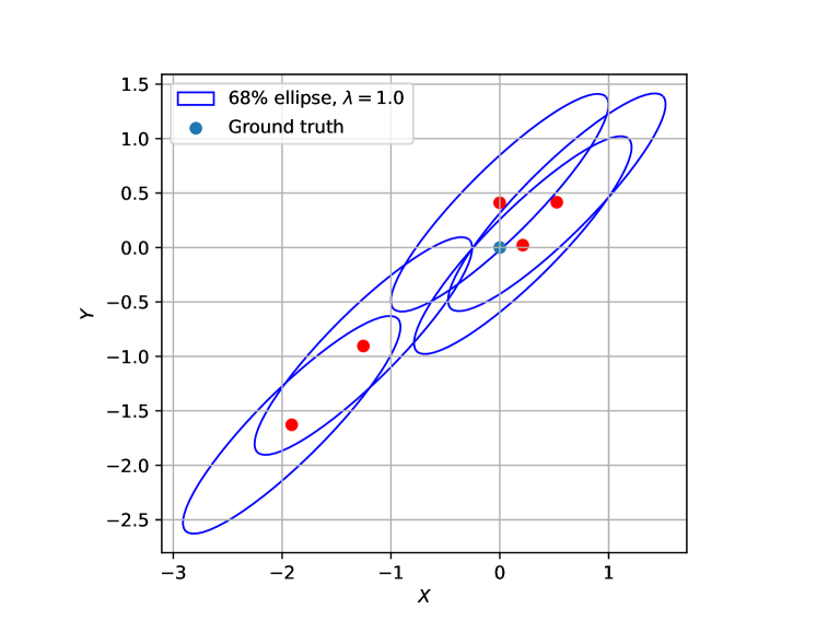
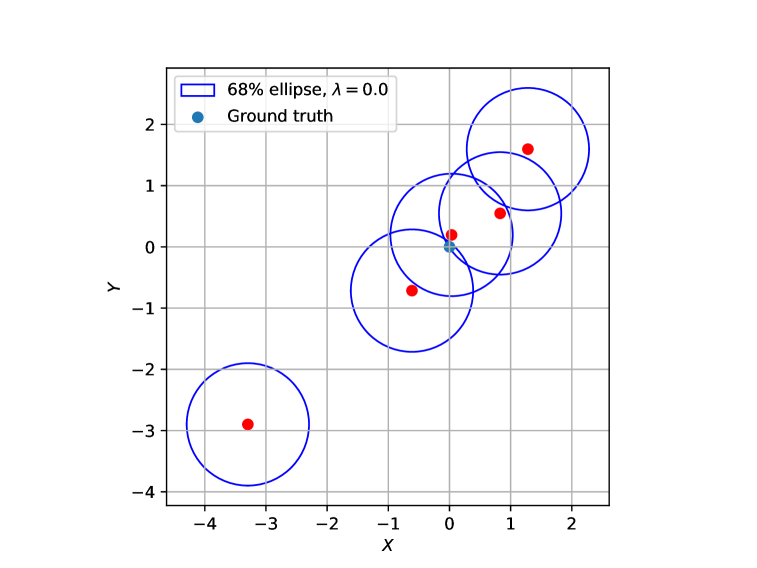
Figure 2: Data points for a pair of observables generated with a nontrivial correlated covariance matrix, shown on the left with their correct error ellipse, and on the right with an error circle in which all correlated uncertainties have been set to zero.

It is important to understand that each datapoint in Fig. 2 corresponds to a different run of the universe. This means that in a real PDF determination only one occurrence is actually realised: it is only within the closure test that one has a distribution of events. This means that our model of inconsistency reproduces both the situation in which an uncertainty has been incorrectly estimated, but also the situation in which datapoints are systematically offset from their true values, because each particular instance of $L_{1}$ data corresponds to a specific value of the nuisance parameter associated to each correlated systematics, i.e. to a systematic shift.

3 Results

We will now present the results of this study. First, we summarise the settings that we have adopted and introduce the three inconsistency scenarios that we have considered, then we present results for each scenario.

3.1 Settings and scenarios

We have performed a number of closure tests with various inconsistency scenarios, starting each time from a baseline consistent closure test. In all cases, for ease of comparison with previous work we adopt the same underlying truth adopted for the closure test of Ref. DelDebbio:2021whr , namely a specific random replica from the NNPDF4.0 set. Individual NNPDF replicas have more structure than the average over replicas, so this choice is somewhat more general than that of any current best-fit PDF. We perform $N_{\rm fit}=25$ closure tests, each based on a different randomly generated set of $L_{1}$ data, and each containing $N_{\rm rep}=100$ replicas. Previous studies NNPDF:2021njg suggest that these sample sizes are sufficient to ensure reliable results; as in these previous references, uncertainties associated to the finite size of the samples will be estimated through a bootstrap procedure (see App. B for details).

We specifically consider three inconsistency scenarios, in each of which we divide the dataset into two subsets, one used for PDF determination (in-sample data) and the other used for testing the accuracy of predictions (out-of-sample data). The two samples are in each case constructed in such a way that the in-sample and out-of-sample datasets are equally representative of the full dataset in terms of kinematics. We furthermore introduce inconsistencies in each case in a different subset of the in-sample data. The scenarios differ in the choice of full dataset and inconsistent dataset. In all cases, the inconsistency is introduced following Eq. (17): the baseline consistent case corresponds to choosing $\lambda=1$, and an increasingly strong inconsistency is introduced by choosing increasingly small values of $\lambda$, until with $\lambda=0$ we end up with a situation similar to that depicted in Fig. 2 (right), in which all correlated uncertainties are set to zero in the covariance matrix used in the PDF determination. Results shown for the statistical indicators follow in all cases the definitions given in Sect. 2.2.

The three scenarios illustrate three possible situations. The first is a determination of PDFs based only on DIS data, in which all the in-sample neutral-current (NC) HERA data are made inconsistent. This illustrates a case of bulk inconsistency, in which the majority of the data that determine the PDFs are inconsistent. The second is a determination based on a global dataset, in which we introduce the inconsistency in a single double-differential Drell-Yan dataset. This is representative of a situation in which the inconsistency is localised in a single, though highly precise and relevant, dataset. The third is again based on a global PDF determination, in which we make single-inclusive jet data inconsistent. This is illustrative of the inconsistency being present in a dataset that almost entirely determines one specific PDF (in this case the gluon at medium $x$).

3.2 Bulk inconsistency: Deep Inelastic Scattering

The first scenario, of a bulk inconsistency, is a PDF determination using DIS data only. The datasets correspond to all the DIS data used for the NNPDF4.0 NNPDF:2021njg PDF determination, with the same kinematic cuts. They are listed in Table 1, where the split between in-sample and out-of-sample is also indicated. The kinematic coverage and data split are displayed in Fig. 3, which shows that the in- and out-of-sample datasets have similar coverage.

Datasets	$N_{\text{data}}$	$R_{b}$
		$\lambda=1.0$	$\lambda=0.7$	$\lambda=0.4$	$\lambda=0.0$
NMC $F_{2}^{d}/F_{2}^{p}$ Arneodo:1996kd	121	0.8	0.7	0.8	1.0
SLAC $F_{2}^{p}$ Whitlow:1991uw	33	0.7	0.7	0.8	1.1
SLAC $F_{2}^{d}$ Whitlow:1991uw	34	0.8	0.8	0.8	0.9
BCDMS $F_{2}^{p}$ Benvenuti:1989rh	333	0.8	0.8	0.8	1.1
BCDMS $F_{2}^{d}$ Benvenuti:1989rh	248	0.9	0.9	0.9	1.1
CHORUS $\sigma_{CC}^{\nu}$ Onengut:2005kv	416	0.8	0.9	0.8	0.9
CHORUS $\sigma_{CC}^{\bar{\nu}}$ Onengut:2005kv	416	0.9	1.0	1.0	1.2
NuTeV $\sigma_{CC}^{\nu}$ (dimuon) Goncharov:2001qe ; MasonPhD	39	0.8	0.9	0.9	1.2
HERA I+II $\sigma_{\rm CC}^{e^{+}p}$ Abramowicz:2015mha	39	0.9	1.0	1.0	1.3
HERA I+II $\sigma_{\rm NC}^{\rm charm}$ H1:2018flt	37	1.0	1.1	1.1	1.2
$(^{*})$ HERA I+II $\sigma_{\rm NC}^{e^{-}p}$ $E_{p}=320$ GeV Abramowicz:2015mha	159	0.9	1.0	1.2	2.2
$(^{*})$ HERA I+II $\sigma_{\rm NC}^{e^{+}p}$ $E_{p}=575$ GeV Abramowicz:2015mha	254	0.8	0.9	1.3	2.4
$(^{*})$ HERA I+II $\sigma_{\rm NC}^{e^{+}p}$ $E_{p}=820$ GeV Abramowicz:2015mha	70	0.8	0.9	1.2	2.3
$(^{*})$ HERA I+II $\sigma_{\rm NC}^{e^{+}p}$ $E_{p}=920$ GeV Abramowicz:2015mha	377	0.9	0.9	1.3	2.4
Total (in-sample)	2576	0.9	1.0	1.1	1.7
NMC $\sigma^{{\rm NC},p}$ Arneodo:1996qe	204	0.9	0.9	1.1	1.6
NuTeV $\sigma_{CC}^{\bar{\nu}}$ (dimuon) Goncharov:2001qe ; MasonPhD	37	0.8	0.9	0.9	1.1
HERA I+II $\sigma_{\rm NC}^{e^{+}p}$ $E_{p}=460$ GeV Abramowicz:2015mha	204	0.9	1.0	1.4	2.7
HERA I+II $\sigma_{\rm CC}^{e^{-}p}$ Abramowicz:2015mha	42	0.9	1.0	1.2	1.4
HERA I+II $\sigma_{\rm NC}^{\rm bottom}$ H1:2018flt	26	0.9	1.0	1.2	1.9
Total (out-sample)	513	0.9	0.9	1.1	1.9
Total	3089	0.9	1.0	1.1	1.6

Table 1: Datasets included in the DIS-only inconsistent closure test. The in-sample datasets are in the upper part and the out-of-sample datasets in the lower part of the table. The inconsistent datasets are denoted by an asterisk and collected at the bottom of the upper part of the table. For each dataset we indicate the number of data points after kinematic cuts, and give the value of the normalised bias $R_{b}$, Eq. (14), obtained in a closure test as a function of $\lambda$. All instances in which $R_{b}>1$ are highlighted in boldface.

The inconsistency is introduced in all of the HERA neutral-current inclusive structure function data, starting with consistent $\lambda=1$ and then with increasingly small $\lambda=0.7,\,0.6,\,0.4,\,0.2,\,0$. The inconsistent datasets are flagged in Table 1 and Fig. 3. The total number of inconsistent datapoints is $N_{\rm inc}=860$ out of $N_{\rm data}=2576$ in-sample datapoints.

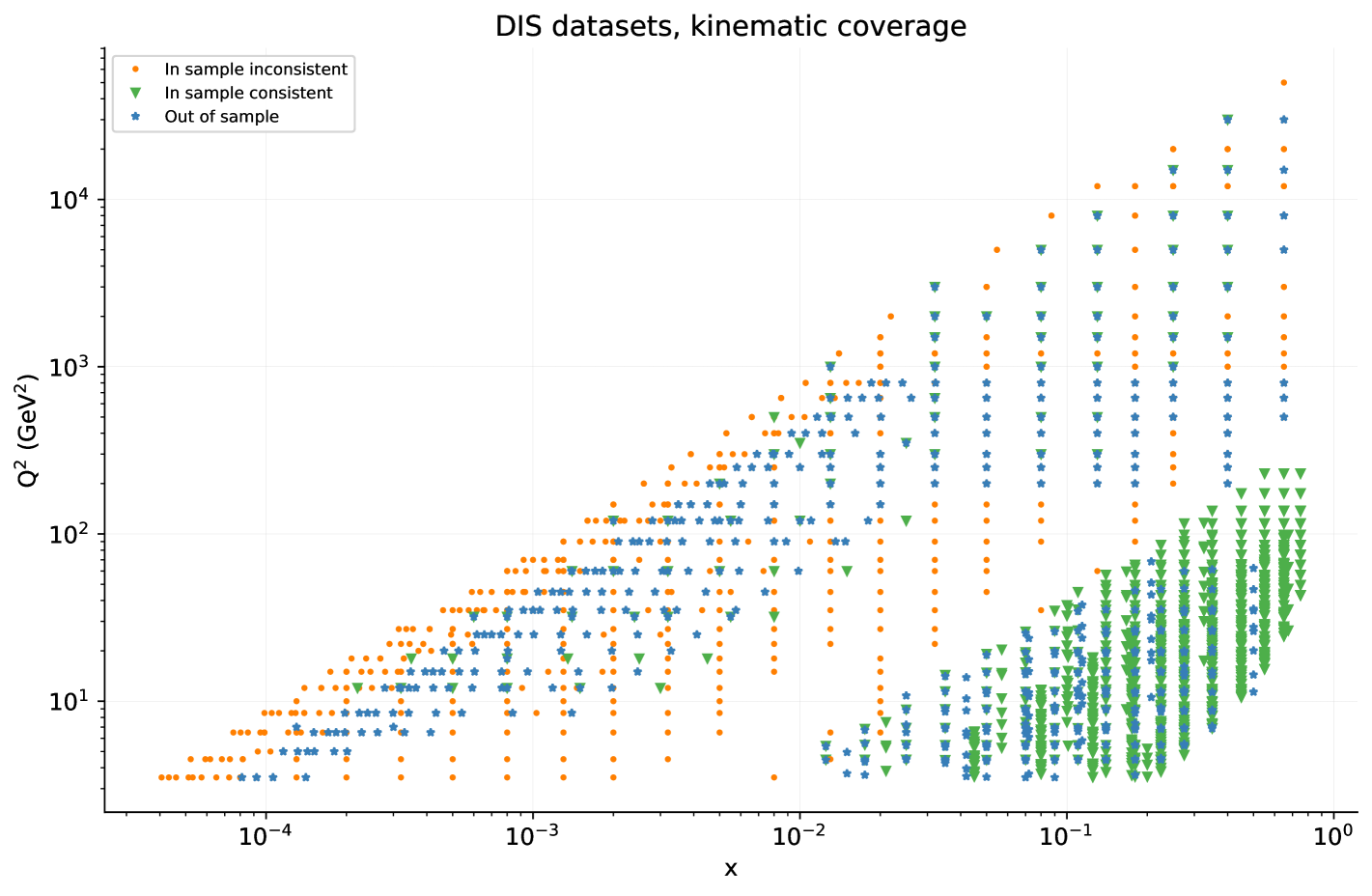
Figure 3: Kinematic coverage of the data of Table 1 in the $(x,Q^{2})$ plane. In-sample consistent data are denoted by green inverted triangles, in-sample inconsistent by orange dots, and out-of-sample by blue stars.

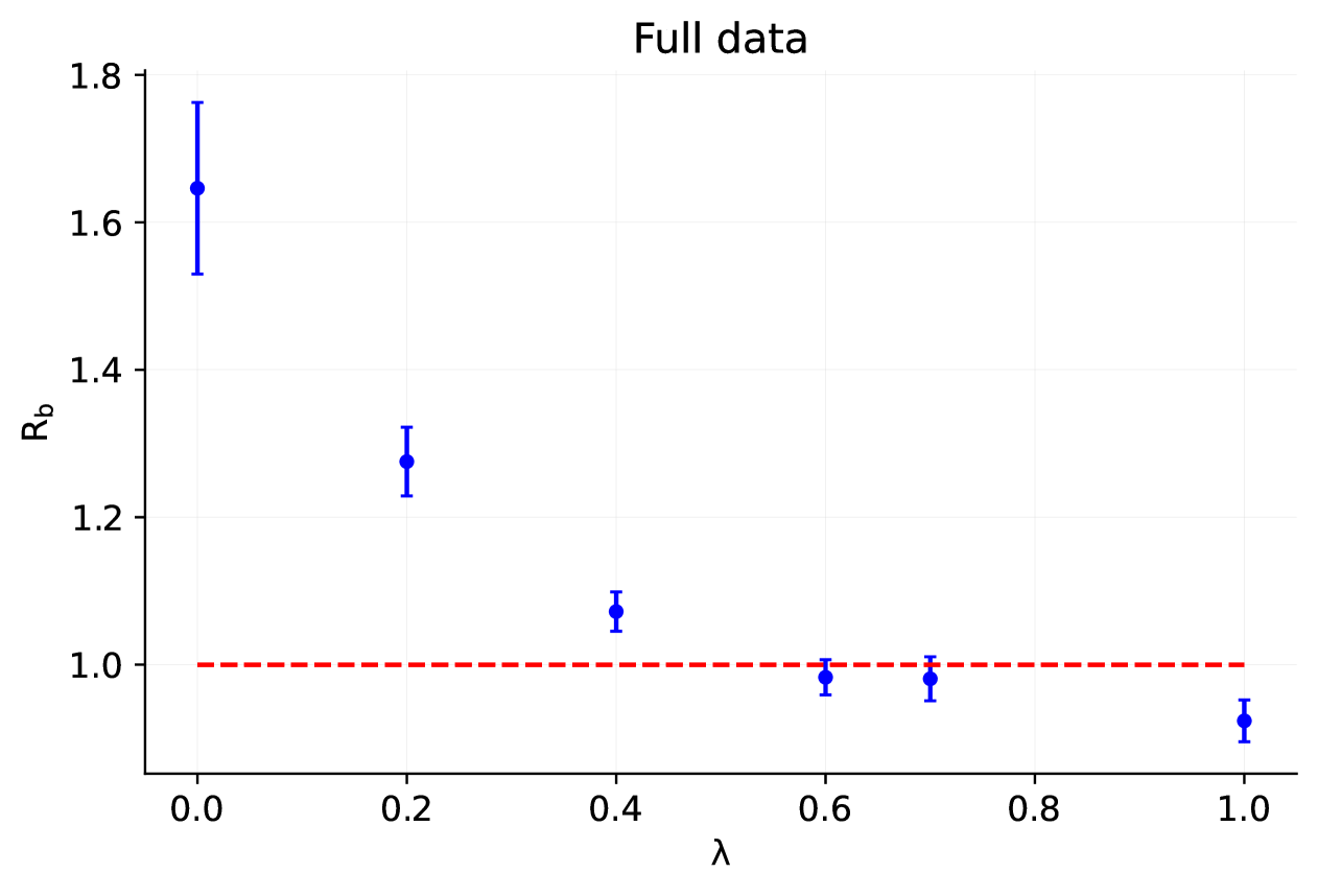
Figure 4: The normalised bias $R_{b}$ Eq. (14), as given in Table 1 for the full dataset (both in-sample and out-of-sample), as a function of $\lambda$. The uncertainty shown reflects the finite size of the replica sample, estimated by bootstrap (see App. B for details).

The values of the normalised bias $R_{b}$, Eq. (14), found in various cases are collected in Table 1 both for all individual datasets and the total dataset. All values for which $R_{b}>1$ are highlighted in boldface. The values for the full dataset are also displayed in Fig. 4 as a function of $\lambda$. The uncertainty on each value is determined by bootstrap (see App. B for details). In Table 2 we also collect the values of the $\xi_{1\sigma}$ quantile estimator Eq. (15). Finally, the normalised distribution of relative differences $\delta_{i}^{(l)}$ Eq. (13) is displayed in Fig. 5 for the fully consistent $\lambda=1$ case, the intermediate case $\lambda=0.4$, and the extreme inconsistency $\lambda=0$.

It is interesting to observe that, in the consistent $\lambda=1$ case, $R_{b}\lesssim 1$, and accordingly $\xi_{1\sigma}\gtrsim 0.68$, indicating that uncertainties are somewhat overestimated. Note that the bias-variance ratio $R_{b}$ was instead found to equal one within uncertainty in Ref. NNPDF:2021njg , however, as mentioned in Sect. 2.2 (see also App. A), the normalised bias is a somewhat more accurate estimator as it is less subject to fluctuations between different datasets.

The most remarkable feature of the behavior of the normalised bias and corresponding quantile estimator for the total dataset is that, contrary to what one might expect, they display very nonlinear behavior when viewed as a function of $\lambda$: for $\lambda\geq 0.4$ they are almost flat, indicating that, despite the inconsistency, PDF uncertainties remain faithful, but then when $\lambda$ approaches zero $R_{b}$ sharply rises and $\xi_{1\sigma}$ rapidly drops, indicating substantial uncertainty underestimate.

$\lambda$	$\xi_{1\sigma}$
1.0	0.72 $\pm$ 0.02
0.7	0.69 $\pm$ 0.02
0.6	0.69 $\pm$ 0.02
0.4	0.64 $\pm$ 0.02
0.2	0.60 $\pm$ 0.02
0.0	0.52 $\pm$ 0.03

Table 2: The $\xi_{1\sigma}$ quantile estimator, Eq. (15), as a function of $\lambda$. The uncertainty shown reflects the finite size of the replica sample, (see App. B for details).

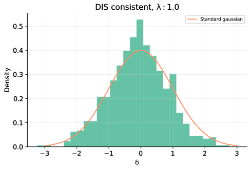
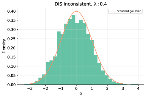
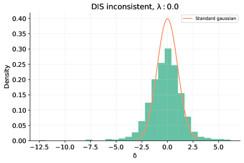
Figure 5: The normalised distribution of relative differences $\delta_{i}^{(l)}$ in the observables space, Eq. (13), for $\lambda=1$ (left), $\lambda=0.4$ (centre) and $\lambda=0$ (right). In all cases, a univariate zero-mean Gaussian distribution is plotted for reference.

Coming now to individual datasets, we can see from Table 1 that for $\lambda>0.4$ essentially all datasets remain consistent, while for $\lambda=0.4$ all in-sample data remain consistent while marginal inconsistency starts appearing both in the inconsistent datasets, as well as in out-of-sample datasets that probe similar kinematics. When $\lambda=0$ almost all in-sample and all out-of-sample datasets display significant inconsistencies. Quite in general, the fact that in-sample and out-of-sample datasets behave in a similar way shows that the model is effective at generalising. To better illustrate the behavior of individual datasets, in Fig. 6 we also show graphically some of the results of Table 1 (with additional values of $\lambda$, to ease visualization).

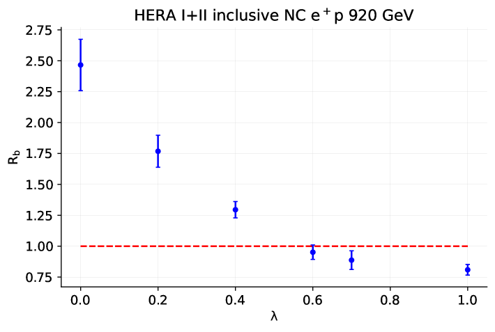
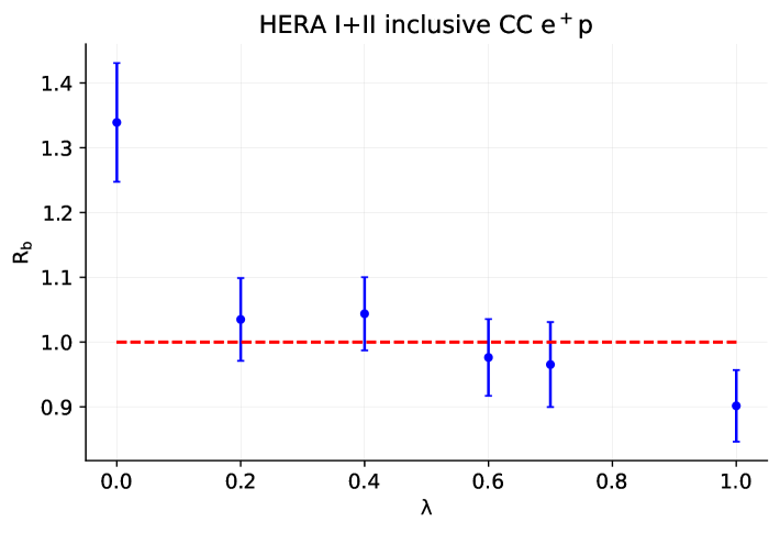
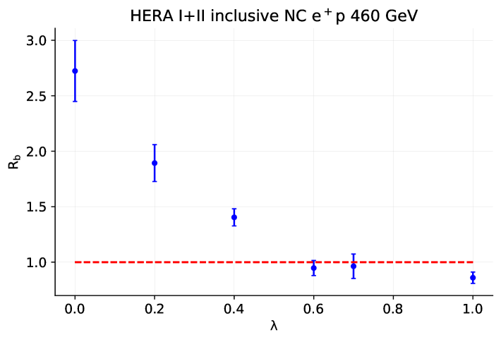
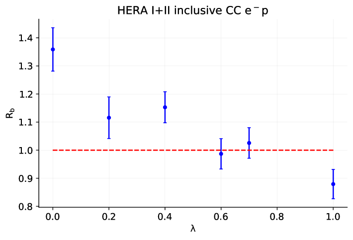
Figure 6: Same as Fig. 4, but now for some individual datasets: HERA I+II $\sigma_{\rm NC}^{e^{+}p}$ $E_{p}=920$ GeV (in-sample, inconsistent, top left); HERA I+II $\sigma_{\rm CC}^{e^{+}p}$ (in-sample, consistent, top right); HERA I+II $\sigma_{\rm NC}^{e^{+}p}$ $E_{p}=420$ GeV and HERA I+II $\sigma_{\rm CC}^{e^{-}p}$ (both out-of-sample, bottom).

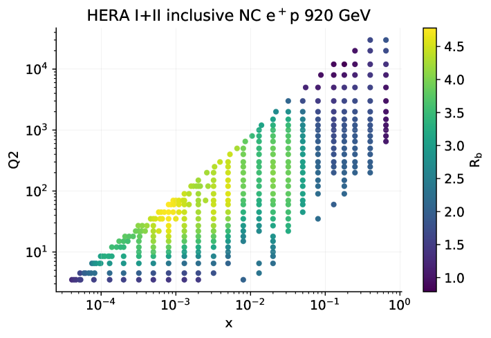
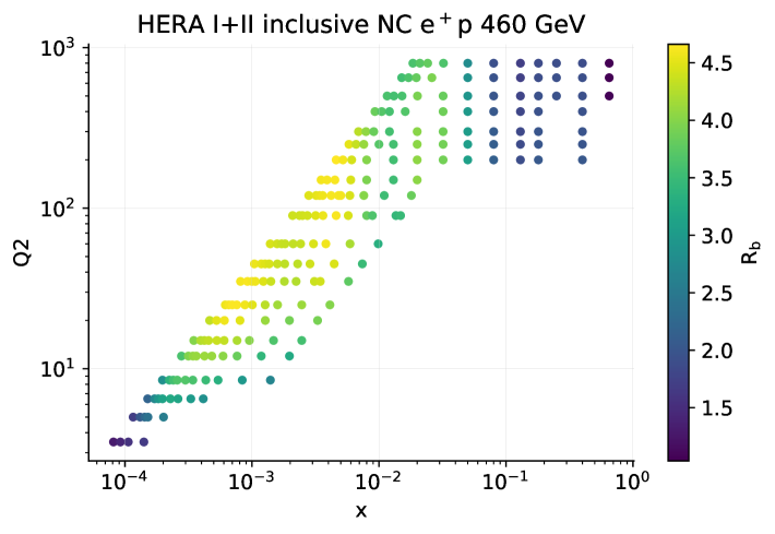
Figure 7: Scatter plot of the normalised bias $R_{b}$ for individual datapoints included in the two HERA I+II $\sigma_{\rm NC}^{e^{+}p}$ datasets shown in the left column of Fig. 6 in the maximally inconsistent scenario ($\lambda=0$): $E_{p}=920$ GeV (left), in-sample, inconsistent and $E_{p}=460$ GeV (right), out-of-sample.

Finally, we look at individual datapoints. This misses the information on PDF-induced correlations, but it allows for a more fine-grained understanding of the behavior of the PDF model. In Fig. 7 we show the normalised bias $R_{b}$ for each datapoint in the maximally inconsistent $\lambda=0$ scenario, for the two HERA I+II dataset $\sigma_{\rm NC}^{e^{+}p}$ datasets shown in the left column of Fig. 6, which are both affected by the inconsistency: $E_{p}=920$ GeV (top left in Fig. 6, left in Fig. 7), in-sample, directly affected, and $E_{p}=460$ GeV (bottom left in Fig. 6, left in Fig. 7), out-of-sample and thus indirectly affected. It is clear that the pattern of inconsistency is quite similar for both datasets. This can be understood by studying the correlation between data and individual PDFs (see App. C): the PDFs that are most strongly correlated to the inconsistent dataset will be affected, and in turn lead to inconsistent predictions for data that are also strongly correlated to them. In this case indeed both datasets are strongly correlated to the gluon (see App. C). It should be noted however that the similarity is also partly due to the fact that in both cases datapoints with $10^{-3}\lesssim x\lesssim 10^{-2}$ have the smallest statistical uncertainties and thus the effect of the inconsistency is more clearly visible.

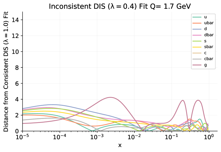
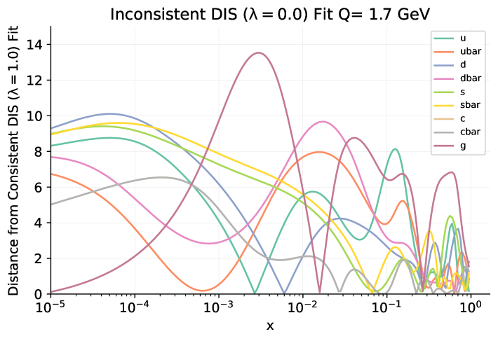
Figure 8: Distance between the PDFs obtained in an inconsistent and consistent fit to the same underlying data. Results are shown for $\lambda=0.4$ (left) and $\lambda=0$ (right).

In conclusion, it is interesting to ask how the PDFs behave upon introducing an inconsistency, both in the case (such as for $\lambda=0.4$) in which the model largely corrects for the inconsistency, and in the case (such as for $\lambda=0$) in which it does not. In Fig. 8 we plot the distance between the central values of all PDFs determined from a consistent and inconsistent fit to the same underlying $L_{1}$ data, which hence correspond to one particular random fluctuation of the data about the true underlying value. In the inconsistent case, the fluctuations are not reflected correctly by the size of the uncertainty used for fitting, which is smaller than what it ought to be. The distance (defined in App. B of Ref. Ball:2014uwa ) is the mean-square difference of central values in units of the standard deviation of the mean, so that $d=1$ corresponds to statistical equivalence; with $N_{\rm rep}=100$ replicas a one-sigma shift corresponds to $d=10$. Results are shown both for $\lambda=0.4$ and $\lambda=0$. It is clear that for $\lambda=0.4$ the PDFs found in a consistent and inconsistent fit are almost statistically equivalent, with at most a localized quarter sigma deviation in the gluon. On the contrary, for $\lambda=0$ there is clear inconsistency.

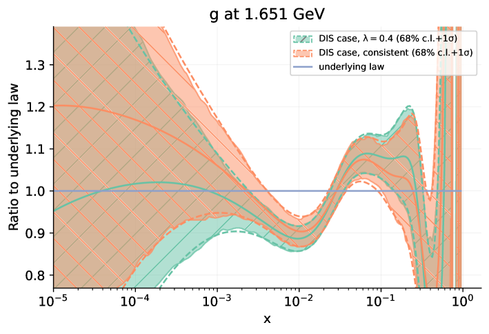
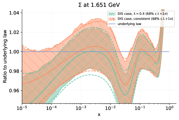
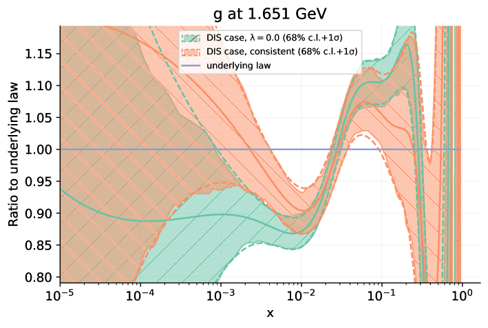
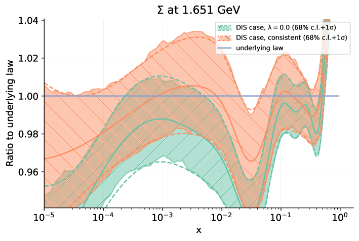
Figure 9: Comparison between the inconsistent and consistent closure test results, shown as a ratio to the true underlying law. The gluon (left) and singlet (right) are shown, for $\lambda=0.4$ (top row) and $\lambda=0$ (bottom row).

This then begs the question of whether the inconsistency is due to shrinking of uncertainties with fixed bias, or increased bias with shrinking uncertainty, or both, and how when $\lambda=0.4$ the model corrects for this. In order to address this question, in Fig. 9 we directly compare the gluon and singlet PDF, shown as a ratio to the true underlying law. It is clear that with $\lambda=0.4$ the model leads to results that are essentially unchanged in comparison to the consistent case, except perhaps a marginal reduction in uncertainty, which explains the increase of $R_{b}$ by about 10% in comparison to the fully consistent case, and a change in the central value of the gluon which is compatible with a statistical fluctuation. When $\lambda=0$ instead, there is a certain shift in central value, but more importantly a significant reduction in uncertainty. This means that, when $\lambda=0.4$, the model does correct for the underestimated uncertainty in the inconsistent data, by not reducing the PDF uncertainty despite the reduced data uncertainty. When $\lambda=0$, it does not and the PDF uncertainty shrinks, resulting in underestimated uncertainties on the PDFs. The behavior of other PDFs is similar, though the largest effects are seen in the gluon and quark singlet combinations.

3.3 Single dataset inconsistency: Drell-Yan

We now consider the full NNPDF4.0 dataset NNPDF:2021njg . This is an extensive global collection of data, which includes, on top of all of the DIS datasets listed in Table 1, also a wide set of hadronic data, which are collected for ease of reference in Tables 3-4. Because we will use the same dataset for the inconsistency scenarios discussed in this section and also in Sect. 3.4 below, which are based on different in-sample and out-of-sample partitions, we indicate in Tables 3-4 whether each dataset is in-sample or out-of-sample, and whether it is affected by an inconsistency, in either of the two scenarios discussed in this section and the next. In all cases the DIS data of Tab. 1 are split between in-sample and out-of-sample as indicated in that table, and always treated as consistent. The kinematic coverage and in- and out-of-sample split for the closure test discussed in this Section are displayed in Fig. 10.

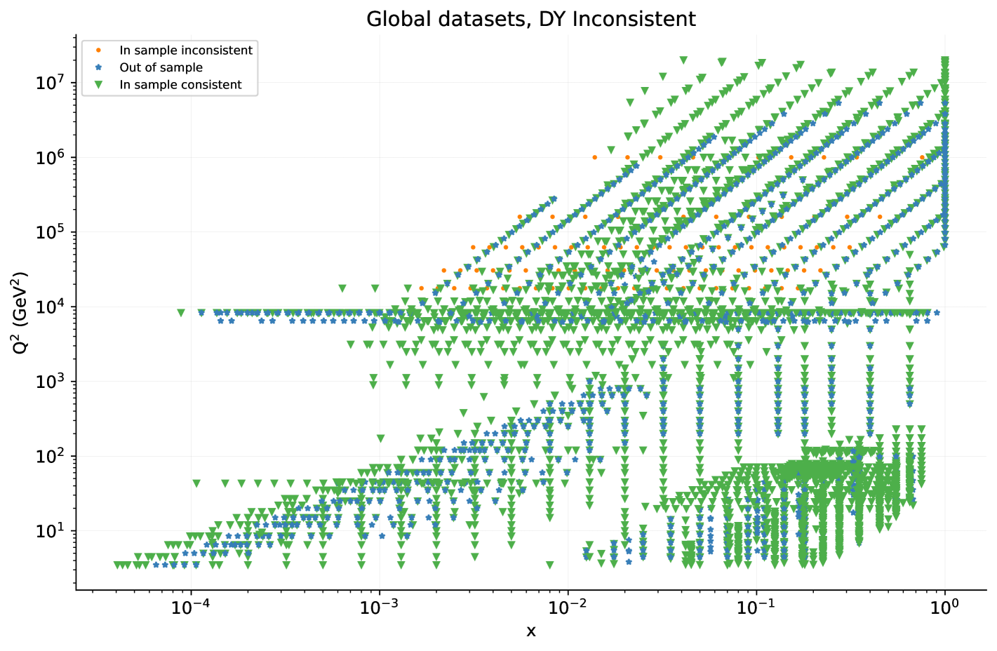
Figure 10: Same as Fig. 3 for the datasets included in the closure test discussed in Sect. 3.3.

Datasets	$N_{\text{data}}$	in/out sample	Inconsistency
DY E866 $\sigma^{p}_{\rm DY}$	29	in
DY E605 $\sigma^{p}_{\rm DY}$	85	in
DY E906 $\sigma^{d}_{\rm DY}/\sigma^{p}_{\rm DY}$ (SeaQuest)	6	in
D0 $Z$ rapidity	28	in
D0 $W\rightarrow\mu\nu$ asymmetry ($\mathcal{L}=7.3$ fb-1)	9	in
ATLAS $W,Z$ 7 TeV ($\mathcal{L}=35$ pb-1)	30	in
ATLAS low mass DY 7 TeV	6	in
ATLAS $W,Z$ 7 TeV ($\mathcal{L}=4.6$ pb-1) CF	15	in
ATLAS low-mass DY 2D 8 TeV	60	in
ATLAS $\sigma_{W,Z}$ 13 TeV	3	in
ATLAS $W^{-}$+jet 8 TeV	15	in
ATLAS $Z$ $p_{T}$ 8 TeV $(p_{T},m_{ll})$	44	in
ATLAS $Z$ $p_{T}$ 8 TeV $(p_{T},y_{Z})$	48	in
CMS $W$ electron asymmetry 7 TeV	11	in
CMS DY 2D 7 TeV	110	in
CMS $W$ rapidity 8 TeV	22	in
LHCb $Z\rightarrow ee$ 7 TeV	9	in
LHCb $Z\rightarrow ee$ 8 TeV ($\mathcal{L}=2$ fb-1)	17	in
LHCb $W,Z\rightarrow\mu$ 8 TeV	30	in
ATLAS high-mass DY 2D 8 TeV	48	in	$\checkmark^{\text{DY}}$
ATLAS $W,Z$ 7 TeV ($\mathcal{L}=4.6$ pb-1) CC	46	out${}^{\text{JETS}}\,$ in${}^{\text{DY}}$
DY E866 $\sigma^{d}_{\rm DY}/2\sigma^{p}_{\rm DY}$ (NuSea) H1:2018flt	15	out${}^{\text{JETS}}\,$ in${}^{\text{DY}}$
CDF $Z$ rapidity	28	out${}^{\text{JETS}}\,$ in${}^{\text{DY}}$
CMS $Z$ $p_{T}$ 8 TeV	28	in${}^{\text{JETS}}\,$ out${}^{\text{DY}}$
LHCb $Z\rightarrow ee$ 13 TeV	16	out

Table 3: Hadronic data entering the global NNPDF4.0 dataset, and used together with the DIS data of Table 1 for the closure tests of Sects. 3-4. On top of the number of datapoints we indicate whether each dataset has been included in or out of sample, and whether it is affected by an inconsistency, with DY denoting the closure test of Sect. 3.3 and JETS denoting the closure test of Sect. 3.4.

Datasets	$N_{\text{data}}$	in/out sample	Inconsistency
ATLAS dijets 7 TeV, R=0.6	90	in
ATLAS direct photon production 13 TeV	53	in
ATLAS single $t$ $R_{t}$ 7 TeV	1	in
ATLAS single $t$ $R_{t}$ 13 TeV	1	in
ATLAS single $t$ 7 TeV ($1/\sigma d\sigma/dy_{t}$)	3	in
ATLAS single $t$ 7 TeV ($1/\sigma d\sigma/dy_{\bar{t}}$)	3	in
ATLAS single $t$ 8 TeV ($1/\sigma d\sigma/dy_{\bar{t}}$)	3	in
ATLAS $\sigma_{tt}^{\rm tot}$ 13 TeV ($\mathcal{L}=139$ fb-1)	1	in
ATLAS $t\bar{t}$ $l+\text{jets}$ 8 TeV ($1/\sigma d\sigma/dy_{t}$)	4	in
ATLAS $t\bar{t}$ $l+\text{jets}$ 8 TeV ($1/\sigma d\sigma/dy_{t\bar{t}}$)	4	in
ATLAS $t\bar{t}$ $2l$ 8 TeV ($1/\sigma d\sigma/dy_{t\bar{t}}$)	4	in
CMS dijets 7 TeV	54	in
CMS $\sigma_{tt}^{\rm tot}$ 7, 8, 13 TeV	3	in
CMS $t\bar{t}$ $l+\text{jets}$ 8 TeV ($1/\sigma d\sigma/dy_{t\bar{t}}$)	9	in
CMS $t\bar{t}$ $2l$ 13 TeV ($d\sigma/dy_{t}$)	10	in
CMS $t\bar{t}$ $l$+ jets 13 TeV ($d\sigma/dy_{t}$)	11	in
CMS single $t$ 7 TeV ($\sigma_{t}+\sigma_{\bar{t}}$)	1	in
CMS single $t$ 8 TeV $R_{t}$	1	in
CMS single $t$ 13 TeV $R_{t}$	1	in
ATLAS single-inclusive jets 8 TeV, R=0.6	171	in	$\checkmark^{\text{JETS}}$
LHCb $W,Z\rightarrow\mu$ 7 TeV	29	out
LHCb $Z\rightarrow\mu\mu$ 13 TeV	15	out
ATLAS $W^{+}$+jet 8 TeV	15	out
CMS $W$ muon asymmetry 7 TeV	11	out
ATLAS $\sigma^{tot}_{tt}$ 7 TeV	1	out
ATLAS $\sigma^{tot}_{tt}$ 8 TeV	1	out
ATLAS single $t$ 8 TeV ($1/\sigma d\sigma/dy_{t}$)	3	out
CMS $\sigma_{tt}^{\rm tot}$ 5 TeV	1	out
CMS $t\bar{t}$ 2D $2l$ 8 TeV ($1/\sigma d\sigma/dy_{t}dm_{t\bar{t}}$)	15	out
CMS single-inclusive jets 8 TeV	185	out∗

Table 4: Table 3 continued.

We consider the case in which the inconsistency is introduced in a single dataset, namely the double differential high-mass Drell-Yan cross section at LHC measured by ATLAS at $\sqrt{s}=8\,\text{TeV}$ Aad:2016zzw . As for the DIS case, we introduce different degrees of inconsistency, parametrized by the value of $\lambda$. The total number of in-sample datapoints is $N_{\text{data}}=3772$ , while the dataset which is made inconsistent only includes $N_{\text{inc}}=48$ datapoints. However, because all correlated uncertainties affecting this data are affected by the inconsistency, and some of them (such as the luminosity uncertainty) are actually correlated to other datasets, the total number of data that are affected by the inconsistency, at least to some extent, is $N_{\text{tot, inc}}=607$.

The values of the normalised bias $R_{b}$ are collected in Table 5, with values for which $R_{b}>1$ highlighted in boldface. We show values for all of the out-of-sample data, for the inconsistent in-sample ATLAS data, and only for the consistent in-sample data for which $R_{b}>1$ for at least one value of $\lambda$. The values of $R_{b}$ for the full dataset are plotted as a function of $\lambda$ in Fig. 11, the values of the $\xi_{1\sigma}$ are in Table 6 and the normalised distribution of relative differences $\delta_{i}^{(l)}$ is in Fig. 12 for the fully consistent $\lambda=1$ case, the intermediate case $\lambda=0.4$, and the extreme inconsistency $\lambda=0$.

Datasets	$N_{\text{data}}$	$R_{b}$
		$\lambda=1.0$	$\lambda=0.8$	$\lambda=0.4$	$\lambda=0.0$
DY E866 $\sigma^{p}_{\rm DY}$	29	0.9	0.9	0.9	1.6
ATLAS $W,Z$ 7 TeV ($\mathcal{L}=35$ pb-1)	30	0.7	0.7	0.9	1.6
ATLAS low-mass DY 2D 8 TeV	60	0.8	0.9	0.9	1.8
ATLAS $Z$ $p_{T}$ 8 TeV $(p_{T},m_{ll})$	44	0.9	1.0	1.5	2.8
CMS $Z$ $p_{T}$ 8 TeV	28	0.8	0.9	1.0	1.7
(*) ATLAS high mass DY 8 TeV ATLAS_2016	48	0.9	1.0	1.3	2.5
Total (in-sample)	3772	0.8	0.9	0.9	1.5
HERA I+II $\sigma_{\rm CC}^{e^{+}p}$ Abramowicz:2015mha	39	0.9	1.0	1.0	1.1
HERA I+II $\sigma_{\rm NC}^{e^{\pm}p}$ $E_{p}=575$ GeV Abramowicz:2015mha	254	0.7	0.7	0.8	0.8
NMC $F_{2}^{d}/F_{2}^{p}$ Arneodo:1996kd	121	0.9	0.9	0.9	0.8
NuTeV $\sigma_{CC}^{\nu}$ (dimuon) Goncharov:2001qe ; MasonPhD	39	1.0	1.1	1.1	1.1
LHCb $W,Z\rightarrow\mu$ 7 TeV LHCb:2015okr	29	0.9	0.9	1.0	1.4
LHCb $Z\rightarrow\mu\mu$ 13 TeV LHCb:2016fbk	15	0.9	0.9	1.0	1.1
ATLAS $W^{+}$+jet 8 TeV ATLAS:2017irc	15	0.7	0.7	1.0	1.5
CMS $W$ muon asymmetry 7 TeV CMS:2013pzl	11	0.7	0.7	0.7	0.8
ATLAS $\sigma^{tot}_{tt}$ 8 TeV ATLAS:2014nxi	1	0.92	0.8	0.9	0.9
ATLAS high mass DY 7 TeV ATLAS:2013xny	5	0.3	0.4	0.7	1.6
ATLAS single $t$ 8 TeV ($1/\sigma d\sigma/dy_{t}$) ATLAS:2017rso	3	0.9	0.9	0.8	0.9
CMS $\sigma_{tt}^{\rm tot}$ 5 TeV CMS:2017zpm	1	0.8	0.8	0.9	0.7
CMS $t\bar{t}$ 2D $2l$ 8 TeV ($1/\sigma d\sigma/dy_{t}dm_{t\bar{t}}$) CMS:2017iqf	15	0.7	0.7	0.8	0.8
CMS single-inclusive jets 8 TeV CMS:2016lna	185	0.7	0.7	0.7	0.9
Total (out-sample)	734	0.9	0.9	1.0	1.3
Total	4506	0.9	0.9	1.0	1.2

Table 5: Normalised bias $R_{b}$, Eq. (14), as a function of $\lambda$, for the closure test discussed in Sect. 3.3. As in Table 1, the in-sample datasets are in the upper part and the out-of-sample in the lower part of the table, with the inconsistent datasets denoted by an asterisk and collected at the bottom of the upper part of the table. Only the in-sample datasets for which $R_{b}>1$ for at least one value of $\lambda$ are included.

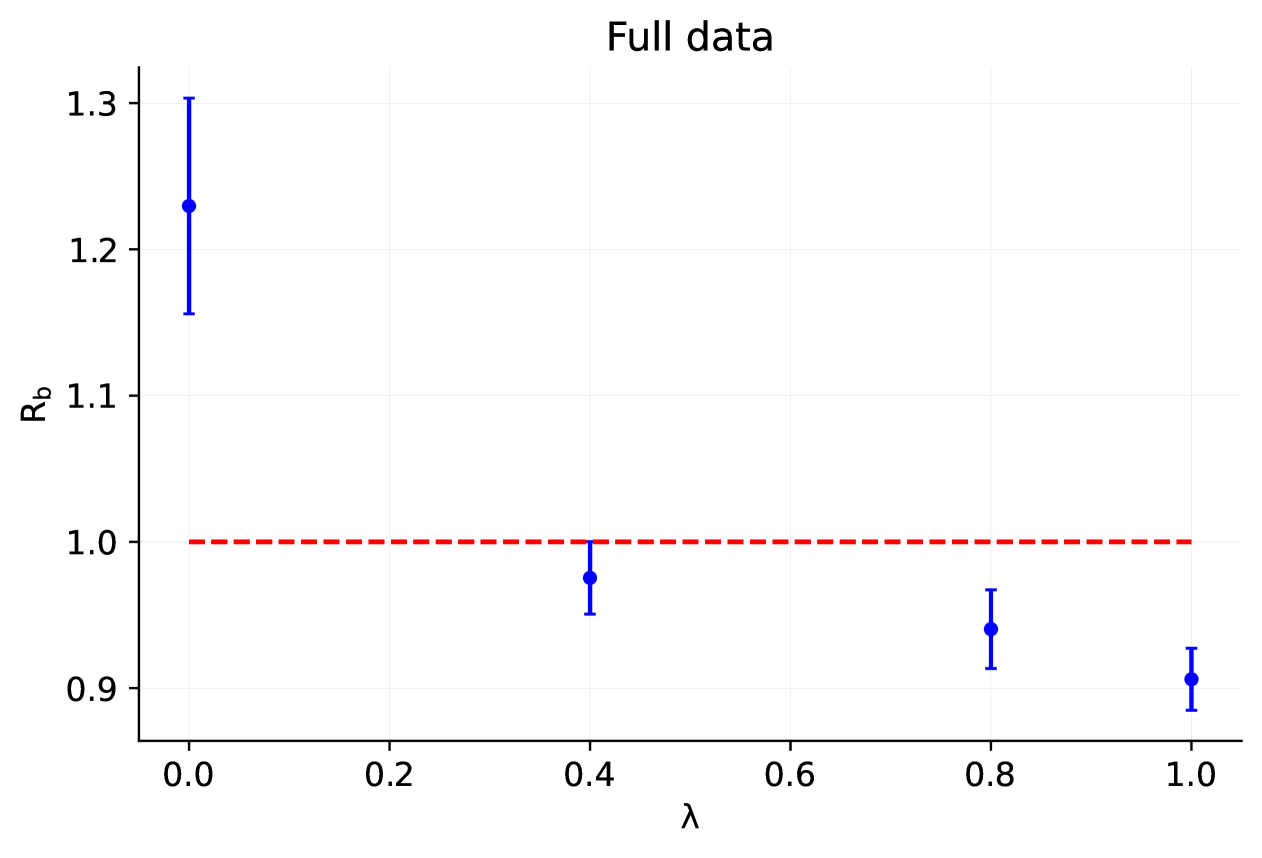
Figure 11: Same as Fig. 4 for the closure test of Sect. 3.3.

$\lambda$	$\xi_{1\sigma}$
$1.00$	$0.74\pm 0.02$
$0.80$	$0.71\pm 0.02$
$0.40$	$0.69\pm 0.02$
$0.00$	$0.63\pm 0.03$

Table 6: Same as Table 2 for the closure test of Sect. 3.3.

The same qualitative behaviour that was seen in the closure test of Sect. 3.2 is observed: namely, for $\lambda\gtrsim 0.4$ the model largely corrects for the inconsistency and all the estimators are qualitatively similar in the consistent and inconsistent case, while when $\lambda=0$ the inconsistency shows up clearly. Quite in general, even in the most inconsistent case, the effect of the inconsistency is milder than in the case discussed in the previous Sect. 3.2, as is especially clear comparing the distribution of relative differences $\delta_{i}^{(l)}$ Eq. (13) respectively shown in Fig.5 and in Fig.12.

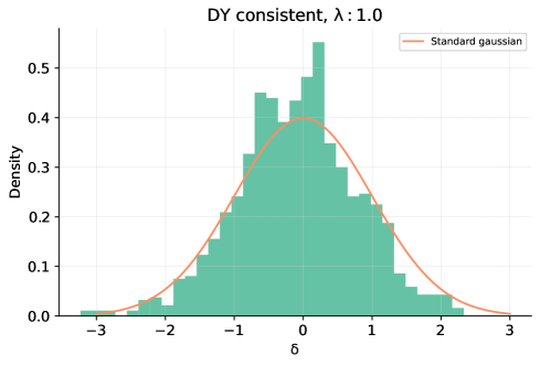
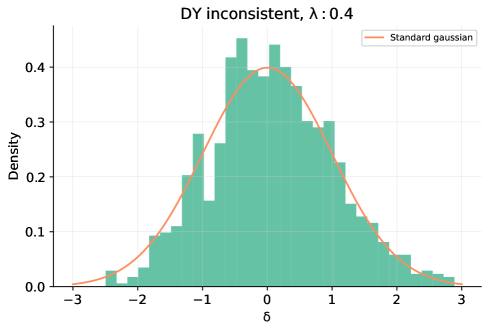
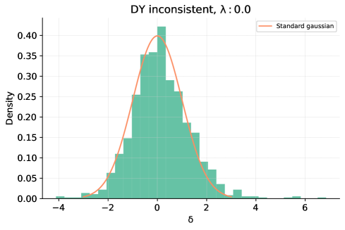
Figure 12: Same as Fig. 5 for the closure test of Sect. 3.3.

Looking at individual datasets, the normalised bias $R_{b}$ remains below one and thus faithful for almost all datasets even with $\lambda=0.4$, the only exceptions being the dataset which is made inconsistent, and one particular Drell-Yan transverse momentum distribution, which starts showing some degree of inconsistency. Interestingly, all out-of-sample datasets remain faithful, with two marginal exceptions of $R_{b}\sim 1.1$, meaning that the inconsistency has not affected the reliability of predictions. Specifically, the out-of-sample ATLAS $\sqrt{s}=7$ TeV DY dataset, which is closely related to the inconsistent dataset, and indeed shows the higher degree of inconsistency in the maximally inconsistent $\lambda=0$ case, remains completely consistent when $\lambda=0.4$.

We finally look specifically at the inconsistent dataset and the out-of-sample dataset which displays the largest inconsistency in the maximally inconsistent $\lambda=0$ case, namely the aforementioned ATLAS $\sqrt{s}=7$ TeV DY dataset. For these datasets in Fig. 13 we show the normalised bias as a function of $\lambda$, and in Fig. 14 the normalised bias for each individual datapoint. The behaviour of the normalised bias as a function of $\lambda$ for these datasets is in fact quite similar to that of the full dataset shown in Fig. 11. This means that the model generalises well, with no significant difference between in-sample, out-of-sample data that are most correlated to the in-sample ones, and the rest of the data.

The behaviour of the normalised bias for individual datapoints shows that both in sample and out of sample the largest inconsistency is found in the low-mass bins and the region $10^{-2}\lesssim x\lesssim 10^{-1}$. In this region, the data are most strongly correlated to the antiquark distributions (see App. C), which are thus driving the inconsistent behaviour.

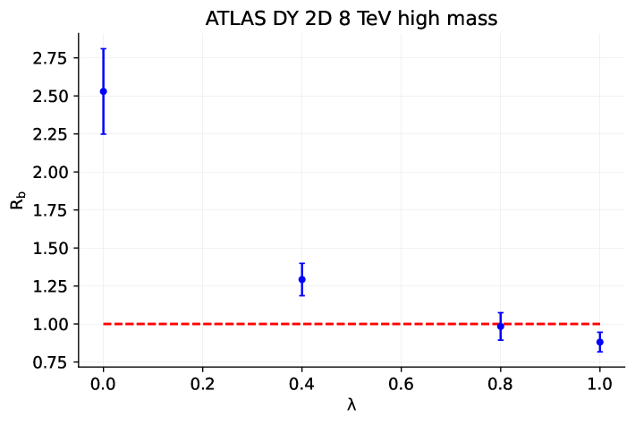
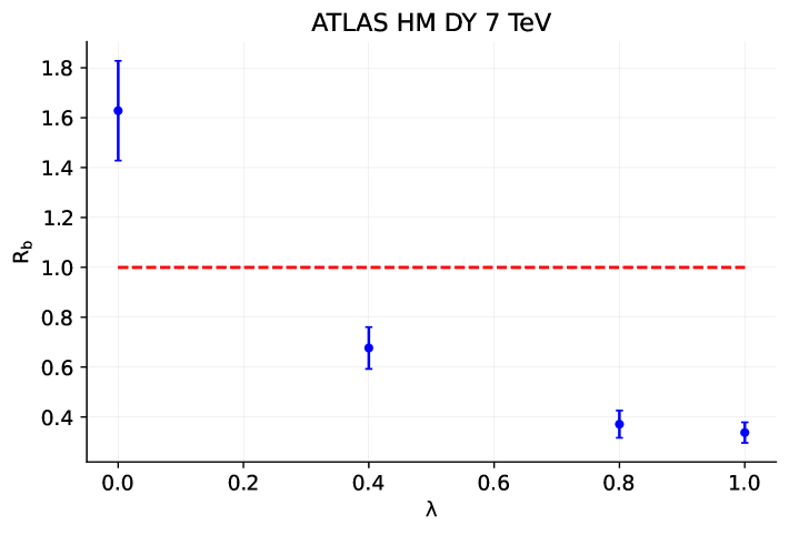
Figure 13: Same as Fig. 11 but now for the inconsistent ATLAS $\sqrt{s}=8$ TeV DY dataset (left) and the ATLAS $\sqrt{s}=7$ TeV DY dataset which shows the largest out-of-sample inconsistency when $\lambda=0$ (right).

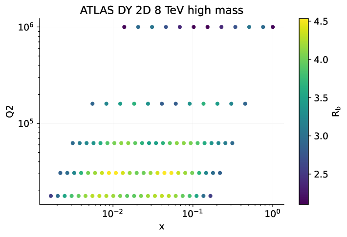
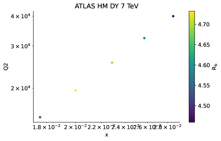
Figure 14: Same as Fig. 7 but for the two datasets shown in Fig. 13 (left and right, respectively).

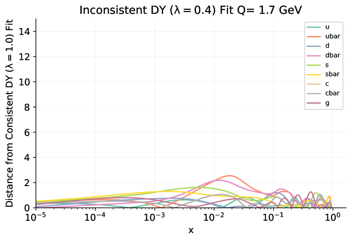
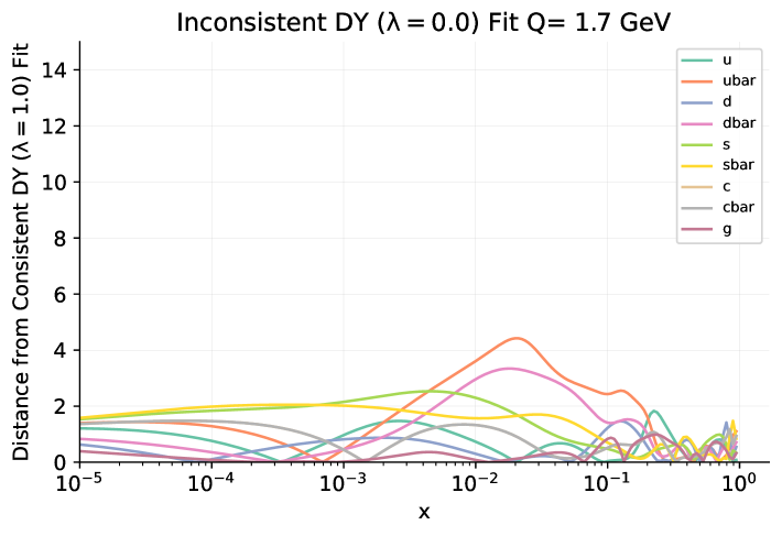
Figure 15: Same as Fig. 8 for the closure test of Sect. 3.3.

In order to check that this is indeed the case, in Fig. 15 we plot the distance between the central values of all PDFs determined from a consistent and inconsistent fit to the same underlying data, both for $\lambda=0.4$ and $\lambda=0$. It is clear that when $\lambda=0$ indeed it is the up and down antiquark distributions that display a statistically significant distance from the consistent ones, with all other PDFs being essentially unaffected. On the other hand when $\lambda=0.4$ it is clear that there is no statistically significant difference between PDFs found in the consistent and inconsistent cases, so indeed the model is correcting for the inconsistency.

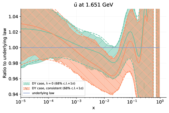
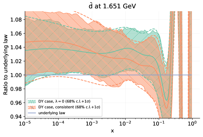
Figure 16: Comparison between the inconsistent and consistent closure test results, shown as a ratio to the true underlying law. The antiup (left) and antidown (right) are shown, in the maximally inconsistent $\lambda=0$ case.

Furthermore, inspection of the PDFs shows that, while when $\lambda=0.4$ the PDFs are essentially unchanged between the consistent and inconsistent case, when $\lambda=0$ (see Fig. 16) the PDF uncertainties are unchanged, but especially the antiup and antidown PDFs undergo a significant shift. The difference in comparison to the case of bulk inconsistency (recall Fig. 9) where the central value moved little but the uncertainty was shrinking can be understood as the consequence of the fact that in that case there was a large amount of different data all controlling the same PDFs (specifically the gluon) and with, in the inconsistent case, underestimated uncertainty, thereby leading to uncertainty reduction. In this case instead there is only one dataset that has a high impact on specific PDFs, with data that are randomly offset by an amount which is larger that their nominal uncertainty. This leads to a corresponding significant offset of the PDFs but without significant uncertainty reduction given the scarcity of the inconsistent data.

3.4 High-impact inconsistency: jets

We finally consider the case in which, as in the previous section, the inconsistency is introduced in a single dataset for a global PDF determination, but now choosing a dataset that has the dominant impact on a specific PDF in a well-defined kinematic region: namely single-inclusive jets that have the dominant impact on the gluon in the intermediate $x$ region.

In particular, we introduce the inconsistency in the ATLAS $\sqrt{s}=8$ TeV single-inclusive jet data Aaboud:2017dvo . The corresponding CMS measurement is kept out-of-sample, so that all the in-sample data for this process are inconsistent. However, the in-sample dataset includes other datasets that are also strongly correlated to the gluon in a similar region, specifically dijet and top pair production. The full in-sample and out-of-sample partition is shown in Tables 3-4, and displayed in Fig. 17. We have $N_{\text{data}}=3793$ in-sample datapoints, with $N_{\text{inc}}=171$ ATLAS inconsistent data, and keeping into account their correlation to other datasets, overall $N_{\text{tot, inc}}=607$ datapoints affected by the inconsistency.

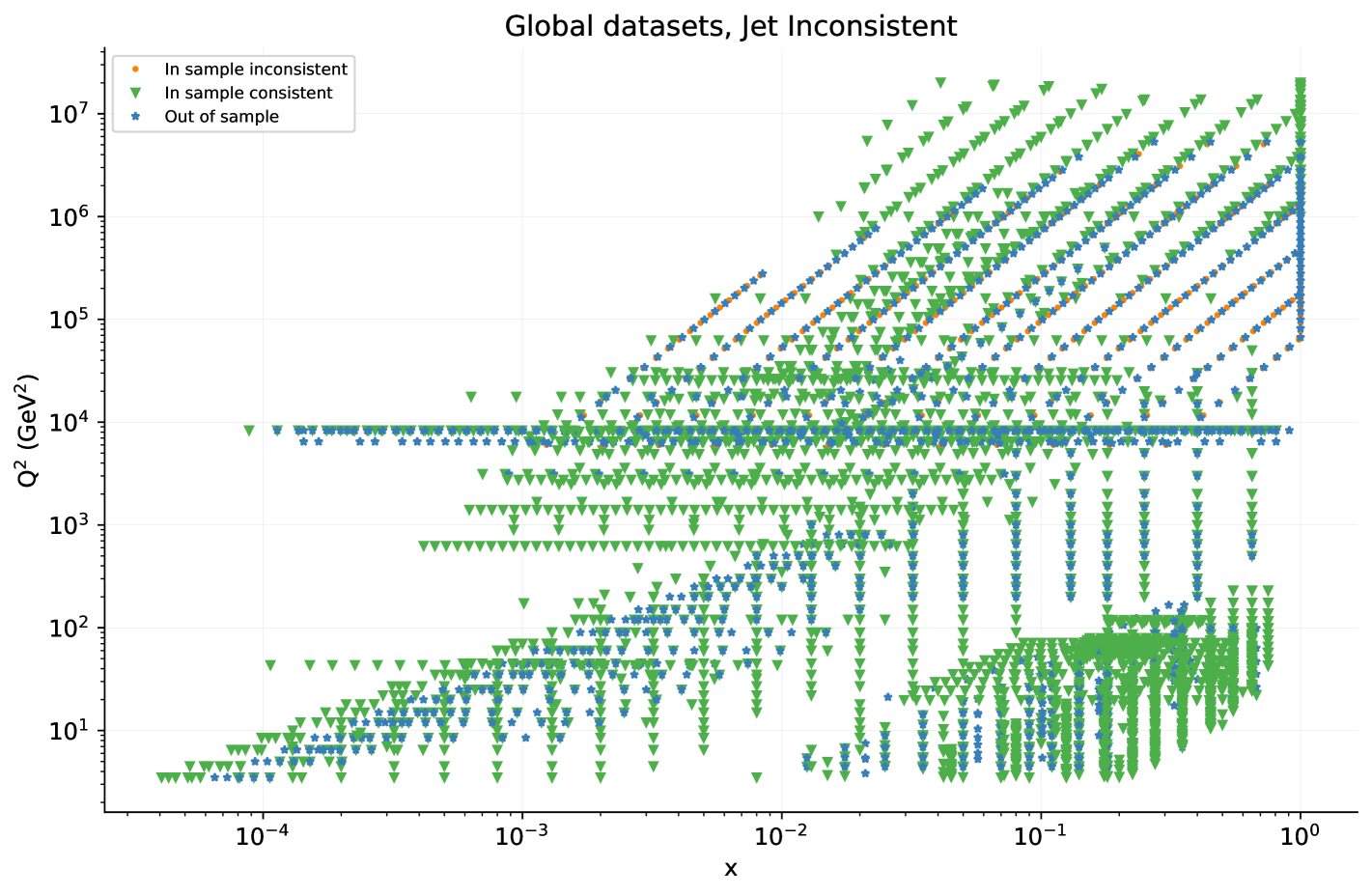
Figure 17: Same as Fig. 3 for the datasets included in the closure test discussed in Sect. 3.4.

Datasets	$N_{\text{data}}$	$R_{b}$
		$\lambda=1.0$	$\lambda=0.6$	$\lambda=0.33$	$\lambda=0.00$
CMS $t\bar{t}\;l+$ jets, 8 TeV ($1/\sigma d\sigma/dy_{tt}$)	10	0.8	0.9	1.0	3.6
ATLAS direct photon production 13 TeV	53	0.8	0.8	1.3	2.0
ATLAS $t\bar{t}\;l+$ jets, 8 TeV ($1/\sigma d\sigma/dy_{tt}$)	5	0.7	0.8	1.0	3.3
NMC $\sigma^{NC,p}$	292	0.9	0.9	1.0	1.6
ATLAS high mass DY 2D 8 TeV	48	0.9	0.9	0.9	1.2
(*) ATLAS jets $8$ TeV, $R=0.6$	171	0.8	0.9	1.1	2.3
Total (in-sample)	3793	0.9	0.9	1.0	2.5
HERA I+II $\sigma_{\rm CC}^{e^{+}p}$ Abramowicz:2015mha	39	1.0	0.8	1.0	1.2
HERA I+II $\sigma_{\rm NC}^{e^{\pm}p}$ $E_{p}=575$ GeV Abramowicz:2015mha	254	0.8	0.8	0.7	1.6
NMC $F_{2}^{d}/F_{2}^{p}$ Arneodo:1996kd	121	0.7	0.7	0.8	0.9
NuTeV $\sigma_{CC}^{\nu}$ (dimuon) Goncharov:2001qe ; MasonPhD	39	0.9	1.0	1.0	1.1
LHCb $W,Z\rightarrow\mu$ 7 TeV LHCb:2015okr	29	0.8	0.9	0.9	1.1
LHCb $Z\rightarrow\mu\mu$ 13 TeV LHCb:2016fbk	15	0.8	0.8	0.8	1.4
ATLAS $W,Z$ 7 TeV ($\mathcal{L}=4.6$ pb-1) CC ATLAS:2016nqi	46	0.7	0.6	0.6	0.9
ATLAS $W^{+}$+jet 8 TeV ATLAS:2017irc	15	0.8	0.8	1.0	3.2
ATLAS high mass DY 7 TeV ATLAS:2013xny	5	1.0	0.9	1.0	1.2
CMS $W$ muon asymmetry 7 TeV CMS:2013pzl	11	0.7	0.7	0.7	0.7
DY E866 $\sigma^{d}_{\rm DY}/2\sigma^{p}_{\rm DY}$ (NuSea) H1:2018flt	15	0.8	0.8	0.8	0.9
CDF $Z$ rapidity CDF:2010vek	15	0.7	0.8	0.7	0.9
ATLAS $\sigma^{tot}_{tt}$ 7 TeV ATLAS:2016nqi	1	0.7	0.8	1.0	5.9
ATLAS $\sigma^{tot}_{tt}$ 8 TeV ATLAS:2017irc	1	0.7	0.7	1.0	5.3
ATLAS single $t$ 8 TeV ($1/\sigma d\sigma/dy_{t}$) ATLAS:2017rso	3	1.0	1.0	1.0	1.5
CMS $\sigma_{tt}^{\rm tot}$ 5 TeV CMS:2017zpm	1	0.7	0.9	1.2	5.4
CMS $t\bar{t}$ 2D $2l$ 8 TeV ($1/\sigma d\sigma/dy_{t}dm_{t\bar{t}}$) CMS:2017iqf	15	0.7	0.8	1.0	4.7
CMS single-inclusive jets 8 TeV CMS:2016lna	185	0.7	0.9	1.1	2.3
Total (out-sample)	823	0.9	0.9	1.0	2.8
Total	4616	0.9	0.9	1.0	2.5

Table 7: Same as Table 5 for the closure test of Sect. 3.4. As in Table 5, only in-sample datasets for which $R_{b}>1$ for at least one value of $\lambda$ are shown.

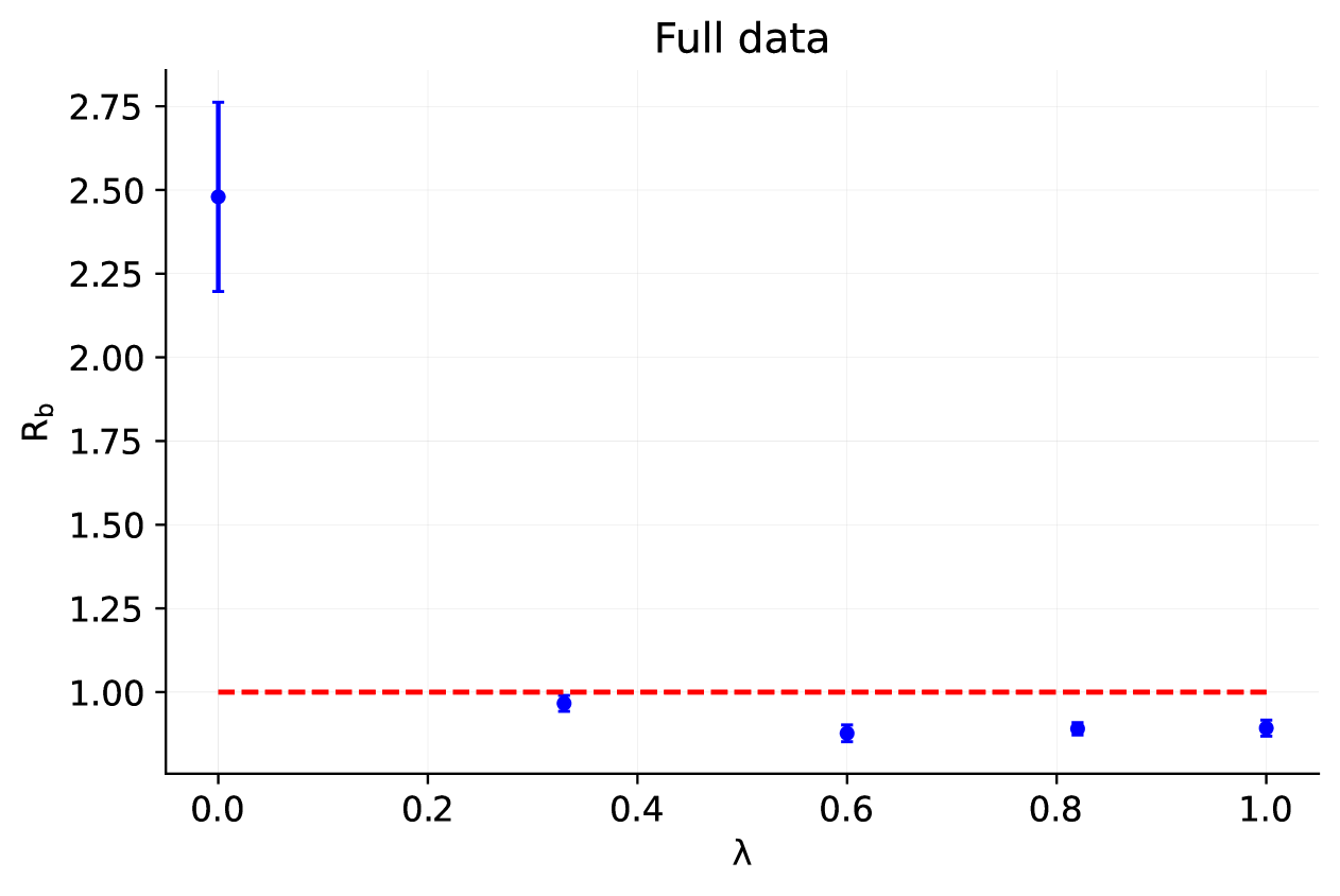
Figure 18: Same as Fig. 4 for the closure test of Sect. 3.4.

The values of the normalised bias $R_{b}$ are collected in Tab. 7. The normalised bias $R_{b}$ is plotted as a function of $\lambda$ in Fig. 18, the values of the quantile $\xi_{1\sigma}$ are collected in Table 8, and the normalised $\delta_{i}^{(l)}$ distribution is shown in Fig. 19 for $\lambda=1$, $\lambda=0.4$, and $\lambda=0$. In this case the dramatic change of behaviour of the normalised bias as $\lambda$ decreases is even more apparent and in fact it extends to even smaller $\lambda$: when $\lambda\gtrsim 0.3$, $R_{b}$ is completely flat and equal to its consistent value, while when $\lambda=0$ it is quite high, in fact even larger than in the case of bulk inconsistency shown in Fig. 4. The same behaviour is displayed by $\xi_{1\sigma}$ and the $\delta_{i}^{(l)}$ distribution.

$\lambda$	$\xi_{1\sigma}$
$1.00$	$0.75\pm 0.02$
$0.82$	$0.74\pm 0.01$
$0.60$	$0.74\pm 0.02$
$0.33$	$0.70\pm 0.02$
$0.00$	$0.45\pm 0.04$

Table 8: Same as Tab. 2 for the closure test of Sect. 3.4.

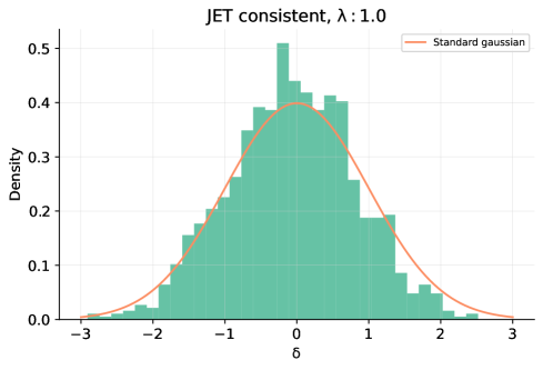
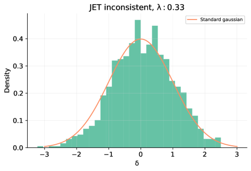
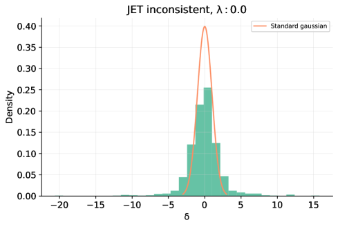
Figure 19: Same as Fig. 5 for the closure test of Sect. 3.4 (but with $\lambda=0.33$ for the central plot).

Coming now to individual datasets, Table 7 shows that when $\lambda\gtrsim 0.3$ the normalised bias is always faithful, with only a marginal sign of inconsistency (with uncertainties underestimated at the 10-20% level) when $\lambda=0.33$, and then only for the inconsistent in-sample dataset, and for a couple out-of-sample datasets that are most strongly correlated to it: specifically the corresponding CMS measurement, and one datapoint for the total top pair production cross section. This indicates that all PDFs are essentially unchanged in this inconsistent case in comparison to the consistent result. On the other hand, when $\lambda=0$ all processes that are highly correlated to the gluon PDF, specifically jets and top pair production (see App. C), and even (though to a lesser extent) HERA DIS data, show large inconsistencies, with uncertainties underestimated by a factor that can be as large as five, indicating large inconsistencies in the gluon PDF.

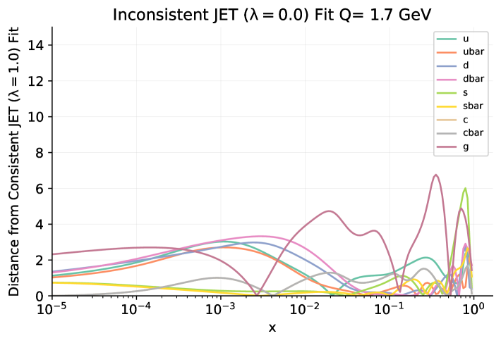
Figure 20: Same as Fig. 8 for the closure test of Sect. 3.4.

This behaviour of the PDFs is indeed seen when determining the distance between results found in the inconsistent and consistent cases (see Fig. 20). When $\lambda=0.33$ (left) all distances are compatible with a statistical fluctuation, while when $\lambda=0$ distances as large as two- or three-sigma are seen for all PDFs. A direct comparison of the gluon PDF (see Fig. 21, left) shows that the large distance is due to the fact that in the inconsistent case the gluon shows a large deviation from its true value, but with no significant increase in its uncertainty in comparison to the consistent case. A similar trend can be observed from the right plot of Fig. 21 in the singlet PDFs, $\Sigma=\sum_{i}(q_{i}+\bar{q}_{i})$, which is directly coupled to the gluon via DGLAP evolution equations, and therefore also shows a sizable deviation from the true value in the inconsistent case, although to the one-sigma level.

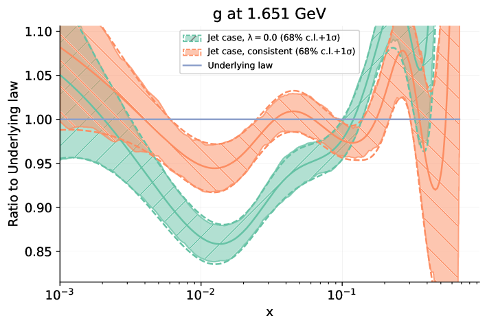
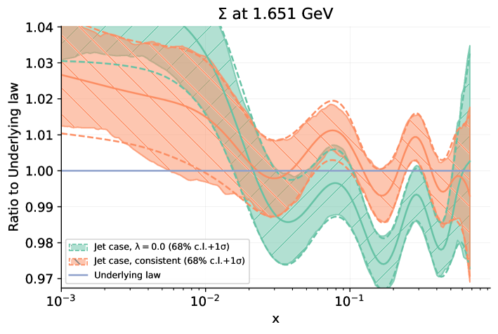
Figure 21: Comparison between the gluon PDF (left) and singlet PDF (right) obtained in the inconsistent and consistent closure tests, shown as a ratio to the true underlying law.

4 Flagging inconsistencies

The main result of the study, presented in Sect. 3, is that in all the scenarios that we investigated the neural net corrects for inconsistencies, leading to faithful uncertainties, unless the inconsistency is extreme. Whereas it is unlikely that extreme inconsistencies such as the one considered in Sect. 3.2 with $\lambda=0$ might be realistic, a situation such as those considered in Sects. 3.3-3.4, in which an individual dataset is severely inconsistent, are well possible. While the specific scenario we examined, in which all correlated uncertainties are missed, is somewhat simplistic, an extreme inconsistency could manifest itself, e.g. if a dominant source of systematics was missed altogether. This then raises the question of whether in such a case the inconsistency could be detected in a real-life scenario.

Clearly, this cannot be done by looking at the normalised bias, given that, as explained in Sect. 2, this quantity can only be computed if the underlying theory is known and more sets of $L_{1}$ data, corresponding to different runs of the universe, are available. Of course, in a real-life situation, the underlying law is not known and only one run of the universe is available via the actual experimental data: so is it possible to detect inconsistent datasets included in a global PDF analysis? In this section we address this question, and use the closure test as a means to optimise a procedure that can be used in a realistic case, taking as a starting point a procedure that was suggested in Ref. NNPDF:2021njg .

4.1 Testing for inconsistencies

In order to construct consistency indicators to be used in an actual PDF fit we consider the closure test of Sect. 3.2, based on $N_{\rm fit}=25$ instances of $L_{1}$ data and we compute $N_{\rm fit}$ independent values of $\chi^{2}_{i}$ for each dataset $i$. Next, we define the $n_{\sigma}$ estimator as the normalised deviation of the $\chi^{2}$ from its mean, i.e.

$$n_{\sigma}^{(i)}=\frac{\chi^{2}_{i}-N_{\rm data}^{(i)}}{\sqrt{2/N_{\rm data}^{(i)}}}\,,$$ (18)

where $i$ is the dataset index (note that the standard deviation is $\sqrt{2/N_{\rm data}}$ because the $\chi^{2}$ Eq. (4) is normalised to the number of datapoints). In a closure test, we define the mean value

$$\mu_{i}=\left\langle n_{\sigma}^{(i)}\right\rangle_{N_{\rm fit}}$$ (19)

of $n_{\sigma}^{(i)}$ over the $N_{\rm fit}$ instances.

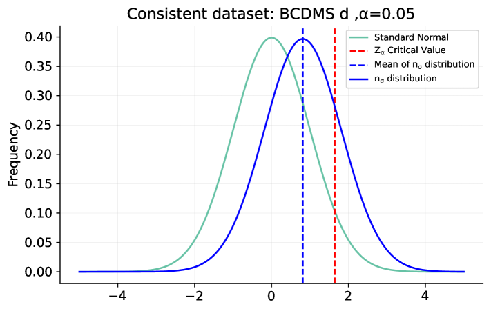
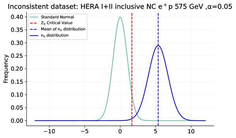
Figure 22: Distribution of $n_{\sigma}$ values in the closure test of Sect. 3.2, with maximal $\lambda=0$ inconsistency. Results are shown both for a consistent and an inconsistent dataset: BCDMS $F_{2}^{d}$ Benvenuti:1989rh (consistent, left panel) and HERA I+II $\sigma_{\rm NC}^{e^{\pm}p}$ $E_{p}=575$ GeV Abramowicz:2015mha (inconsistent, right panel). An univariate standard normal is also shown for comparison with a vertical line indicating its 95% quantile.

We then flag a dataset as inconsistent if the condition $S_{1}$ is satisfied, namely

$$S_{1}:\qquad\mu_{i}>Z,$$ (20)

where $Z$ is some suitable threshold value. Note that we consider $\mu_{i}>0$ because we are interested in flagging cases in which uncertainties are underestimated. Given that the distribution of $n_{\sigma}^{(i)}$ tends to a standard normal in the $N_{\rm data}^{(i)}\rightarrow\infty$ limit, we can think of $Z$ as being approximately a standard normal quantile. In Fig. 22 we display the distribution of $n_{\sigma}^{(i)}$ values found in the closure test of Sect. 3.2 both for a consistent (left) and inconsistent (right) dataset in the case of maximal inconsistency, $\lambda=0$. For reference we also show a standard normal, with a vertical line indicating its 95% confidence quantile.

Clearly, a low value of $Z$ leads to flagging the inconsistency in a larger fraction of cases (true positives, henceforth), but at the cost of also flagging as inconsistent a consistent dataset (false positives, henceforth), and conversely. We accordingly wish to construct a selection procedure that maximises true positives while minimising false positives. Inspection of Fig. 22 suggests that no choice of $Z$ leads to a satisfactory compromise: for instance it is clear from the plot that choosing a 95% confidence level would lead to a very large fraction of false positives, i.e. the consistent BCDMS experiment would be flagged as inconsistent in a significant fraction of cases. This suggests that a more efficient selection criterion is needed, that does not merely rely on the value of $n_{\sigma}$.

4.2 Dataset weighting

In Ref. NNPDF:2021njg it was suggested to detect inconsistencies based on a two-stage procedure. In a first stage, a dataset is flagged as tentatively inconsistent if it satisfies the criterion $S_{1}$, Eq. (20), with a suitable choice of $Z$ (as well as other criteria). In a second stage a new PDF determination is performed, in which the tentatively inconsistent dataset is assigned a large weight, i.e. the loss function Eq. (4) is replaced by the weighted loss

$$\chi^{2}_{\rm weighted}=\frac{1}{N_{\rm data}-N_{\rm data}^{(j)}}\,\sum_{j=1,j\neq i}^{N_{\rm exp}}\,N_{\rm data}^{(j)}\,\chi^{2}_{j}\,+\,w^{(i)}\chi^{2}_{i},$$ (21)

with

$$w^{(i)}=N_{\rm data}/N_{\rm data}^{(i)}.$$ (22)

This means that the putatively inconsistent $i$-th dataset now carries the same weight as all the rest of the data.

If after minimisation the weighted loss remains above threshold, namely if the condition $S_{2}$ is satisfied,

$$S_{2}:\qquad n_{\sigma}^{{\rm weighted},(i)}>Z,$$ (23)

or if the loss $\chi^{2}_{j}$ of any other dataset $j\neq i$ deteriorates more than the given threshold, namely if the condition $S_{3}$ is satisfied,

$$S_{3}:\qquad n_{\sigma}^{{\rm weighted},(j)}-n_{\sigma}^{(j)}>Z\qquad\forall j\neq i,$$ (24)

then dataset $i$ is considered inconsistent. However, if neither condition $S_{2}$ nor $S_{3}$ is satisfied, i.e. if in the weighted fit experiment $i$ is now well reproduced, without significant deterioration of the fit quality for all other experiments, the flag is removed and dataset $i$ is considered consistent. Note that criterion $S_{3}$ is based on the deviation between the weighted and unweighted values of the loss for dataset $j$, rather than its deviation from zero: namely, what is tested is not the absolute consistency of experiment $j$, but rather its compatibility with experiment $i$. Note also that in Ref. NNPDF:2021njg a precise threshold value in Eqs. (23-24) was not specified, and the criterion was applied in a somewhat loose way. Note finally that in principle one might choose a different $Z$ value in each of these equations and also in Eq. (20), though for simplicity we choose a single threshold value.

In the context of a closure test we can assess quantitatively this procedure. To this purpose, we examine the closure test of Sect. 3.2 with $\lambda=0$. Specifically, we consider the HERA I+II $\sigma_{\rm NC}^{e^{\pm}p}$ $E_{p}=575$ GeV Abramowicz:2015mha inconsistent dataset, and the consistent NMC $F_{2}^{d}/F_{2}^{p}$ dataset Arneodo:1996kd . The specific choice of inconsistent dataset is motivated by the fact that the measurement taken with a proton beam energy of $E_{p}=575$ GeV is the least precise of the inconsistent datasets, hence we expect the effect of the inconsistency to be more realistic. We then look at the loss distribution for each of these two datasets over the $N_{\rm fits}$ sets of $L_{1}$ data both in the unweighted case, or when each of them is weighted in turn. In Fig. 23 we plot as a function of the threshold $Z$ the probability of a true negative (consistent experiment not flagged as inconsistent) and of a true positive (inconsistent experiment flagged as inconsistent), when each of the conditions $S_{1}$ Eq. (20), $S_{2}$ Eq. (23) , or $S_{3}$ Eq. (24) is applied separately.

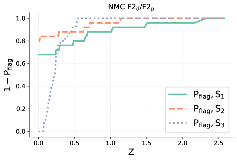
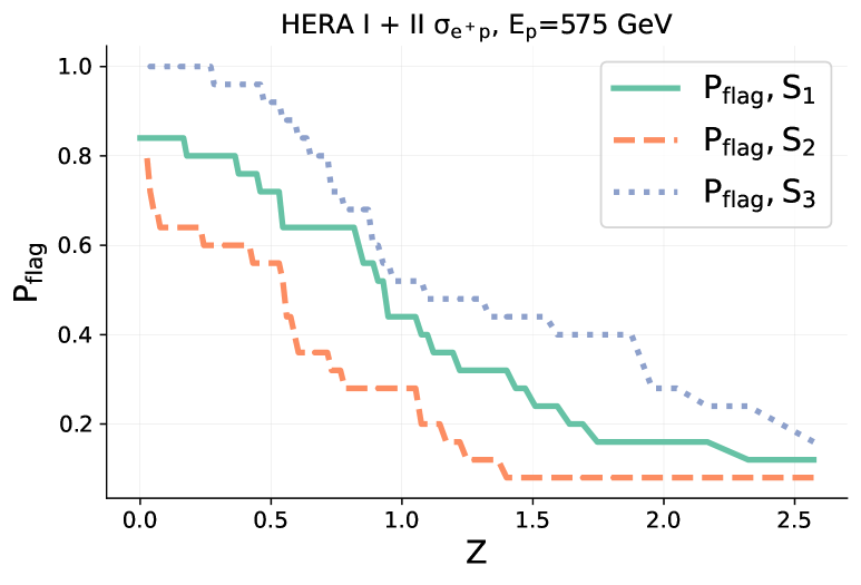
Figure 23: Probability of a true negative (left) and a true positive (right) as a function of the value of the $Z$ threshold. The true negative (consistent experiment not flagged as inconsistent) refers to the NMC $F_{2}^{d}/F_{2}^{p}$ consistent dataset Arneodo:1996kd ; the true positive (inconsistent experiment flagged as such) to the inconsistent HERA I+II $\sigma_{\rm NC}^{e^{\pm}p}$ $E_{p}=575$ GeV dataset Abramowicz:2015mha . The three curves correspond to flagging a dataset as inconsistent when it satisfies either of the three conditions $S_{1}$ Eq. (20), $S_{2}$ Eq. (23) , or $S_{3}$ Eq. (24).

First, we see that indeed, as expected, and discussed at the end of Sect. 4.1, there is a trade-off in that increasing $Z$ increases the probability of true negatives but decreases the probability of true positives, and conversely. Furthermore, we note that condition $S_{2}$ is a more restrictive version of condition $S_{1}$, since giving a higher weight a given dataset can only improve its $\chi^{2}$. Indeed, for fixed $Z$, $S_{2}$ in comparison to $S_{1}$ gives more true negatives, but fewer true positives: effectively, condition $S_{2}$ behaves in a way which is quite similar to that which is obtained using $S_{1}$, but with a larger $Z$ value. Also as noted in Sect. 4.1, neither of these selection criteria seems to lead to a reasonable compromise for any value of $Z$: for instance, choosing $S_{3}$ with $Z\sim 0.5$ (or equivalently $S_{2}$ with $Z\sim 1$) leads to a good fraction of true negatives, around 90%, but an unacceptably small fraction of true positives, smaller than 60% .

On the other hand, selection based on condition $S_{3}$ seems rather more promising, as for most $Z$ values (except very small ones $Z\lesssim 0.5$) it gives both a larger true positive but also a larger true negative rate than conditions $S_{1}$ or $S_{2}$. This suggests that an optimal selection criterion can be constructed by exploiting a suitable combination of criteria that includes condition $S_{3}$.

4.3 Optimal inconsistency detection

As mentioned in Sect. 4.2, in Ref. NNPDF:2021njg it was suggested that inconsistencies could be detected by sequentially applying criteria $S_{1}$ and then $S_{2}$ and $S_{3}$. However, Fig. 23 suggests that a more effective procedure could be to always check for $S_{3}$, even when a dataset has not been flagged as inconsistent by $S_{1}$. Indeed, it is clear from the plot on the left of the figure that, unless a very low value of $Z\lesssim 0.3$ is chosen, there is little chance of $S_{3}$ leading to a false positive even if one does not also require criterion $S_{1}$. On the other hand, whatever the value of $Z$, $S_{3}$ is always more effective in catching true positives.

In order to illustrate this, we compare in Fig. 24 the true and false positive rates based on using three different criteria, namely: flag dataset $i$ as inconsistent if

• $C_{1}$: condition $S_{1}$ is satisfied (same as shown in Fig. 23);

• $C_{2}$: condition $S_{1}$ is satisfied, and in a weighted fit either $S_{2}$ or $S_{3}$ are satisfied (same as in Ref. NNPDF:2021njg );

• $C_{3}$: in a weighted fit either $S_{2}$ or $S_{3}$ are satisfied.

Note that the difference between $C_{2}$ and $C_{3}$ is that in $C_{2}$ a weighted fit is only run for a given dataset when condition $S_{1}$ is satisfied, while in $C_{3}$ a weighted fit is always run for all datasets, and its result are used to flag inconsistencies. Criterion $C_{3}$ is accordingly more computationally intensive as it requires as many weighted fits as there are datasets.

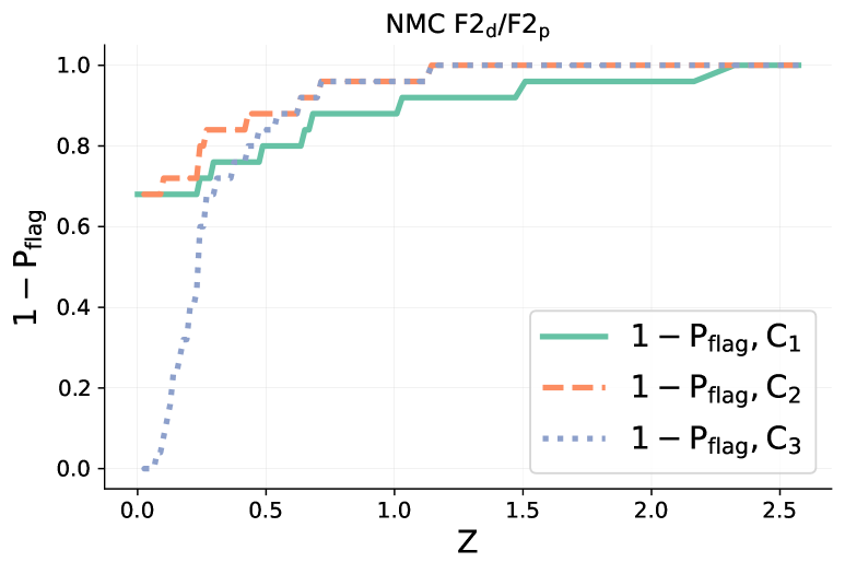
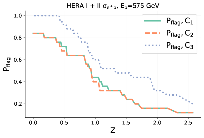
Figure 24: Same ad Fig. 23 but now flagging a dataset as inconsistent using the three criteria $C_{1}$-$C_{3}$ (see text). Criterion $C_{1}$ coincides with $S_{1}$ of Fig. 23, while $C_{2}$ was adopted in Ref. NNPDF:2021njg ).

It is clear that criterion $C_{2}$ used in Ref. NNPDF:2021njg for $Z\gtrsim 0.5$ is somewhat more efficient than purely using criterion $C_{1}$ in terms of true negatives, though equally inefficient in detecting true positives. On the other hand, criterion $C_{3}$ for $Z\gtrsim 0.5$ is equally efficient in detecting true negatives as criteria $C_{1}$ and $C_{2}$, and only fails for very small $Z$ values, where even a small deterioration in fit quality in other datasets upon performing a weighted fit would lead to flagging the dataset as inconsistent. But on the other hand there is a very considerable improvement in efficiency in flagging true negatives, so that for instance a value of $Z\approx 0.5$ would lead to 90% efficiency both for true positive and true negatives.

We conclude that selection based on criterion $C_{3}$ provides a reliable way of identifying genuinely inconsistent datasets. Of course, the precise value of $Z$ should be determined on a case-by-case basis, it will in general depend on the nature of the full global dataset, and should be determined by repeating this analysis for all included datasets with a dedicated closure test.

5 Summary

The possibility that tensions and incompatibilities between experimental measurements may significantly affect the reliability of PDFs and their uncertainty has been often stressed (see e.g. Ablat:2024muy ). In this work, we have investigated this issue using the powerful tool of closure testing, by studying the impact of data inconsistency on PDF determination through the NNPDF methodology in a fully controlled setting. While closure tests had been previously used as a tool to validate the NNPDF methodology, this was done so far assuming perfect theory and fully reliable data uncertainties. The analysis of situations in which an inconsistency is built in the input dataset in a controlled way has enabled us perform this validation under conditions that are closer to real-world situations. Indeed, the scenarios that we have investigated cover a broad spectrum of realistic situations, ranging from bulk inconsistency, in which the majority of the data that determine the PDFs are inconsistent, to an inconsistency localised in a single, though highly precise and relevant, dataset, or a single dataset that almost entirely determines one specific PDF.

Our results demonstrate that the NNPDF methodology manages to correct for moderate to medium inconsistencies, leading to faithful PDFs and uncertainties that generalise correctly to data that are not part of the input dataset, even when they are correlated strongly to the inconsistent data used for PDF determination. Focussing on the effect of inconsistencies of experimental origin, we have learnt that the effect of the inconsistency is visible and distorts the PDFs only when the underestimate of experimental systematic uncertainties is strong, and then only in regions in which experimental measurements are systematics-dominated. We have further developed a procedure in order to detect cases in which uncorrected inconsistencies are present. Taken together, these results provide a reassuring indication that as more data are included in global PDF determination, thereby making PDFs more precise, it will be possible to achieve an accuracy that matches the level of precision.

A natural development of our study is to extend it to more realistic situations, specifically by considering specific critical experimental measurements and systematic uncertainties through a direct involvement of the experimental community. The other natural line of development is to use the same technique to study the impact of inconsistencies of theoretical rather than experimental origin, specifically the fact that predictions are always obtained through a truncation of perturbation theory, thereby leading to systematic shifts whose size is difficult to estimate reliably. These developments will be the object of future studies. In fact, the flexibility of the closure test methodology and the public availability of the NNPDF code NNPDF:2021uiq will facilitate these studies by any interested party.

Appendix A The normalized bias and the bias-variance ratio

The main estimator that we used in this work in order to assess the faithfulness of uncertainties is the normalised bias $R_{b}$ defined in Eq. (14). This differs from the bias-variance ratio used as an estimator in previous studies Ball:2014uwa ; NNPDF:2021njg ; DelDebbio:2021whr . The bias-variance ratio is defined by first introducing the bias and variance, respectively given by (using the notation of Sect. 2.2)

$$B^{(l)}(C) =\left(\mathbb{E}_{\epsilon}{\cal G}(u_{*,k})-f\right)^{T}C^{-1}\left(\mathbb{E}_{\epsilon}{\cal G}(u_{*,k})-f\right),$$ (25)

$$V^{(l)}(C) =\mathbb{E}_{\epsilon}\left[\left(\mathbb{E}_{\epsilon}{\cal G}(u_{*,k})-{\cal G}(u_{*,k})\right)^{T}C^{-1}\left(\mathbb{E}_{\epsilon}{\cal G}(u_{*,k})-{\cal G}(u_{*,k})\right)\right].$$ (26)

One can then define a bias-variance ratio for the $l$-th instance of $L_{1}$ data

$$R^{(l)}_{bv}=\frac{B^{(l)}(C)}{V^{(l)}(C)},$$ (27)

and the bias-variance ratio indicator is then the average root-mean square bias-variance ratio, namely

$$R_{bv}=\sqrt{\frac{\mathbb{E}_{\eta}B^{(l)}(C)}{\mathbb{E}_{\eta}V^{(l)}(C)}}.$$ (28)

Note that if one replaces the experimental covariance matrix $C$ with the average PDF covariance matrix $\overline{C}_{\rm PDF}$ Eq. (11) then the bias-variance ratio coincides with the normalised bias. In fact, the bias-variance ratio for the $l$-th instance is given by

$$R_{bv}^{(l)}(\overline{C})=\frac{1}{N_{\rm data}}\sum_{i=1}^{N_{\rm data}}\frac{(\hat{\Delta}^{(l)}_{i})^{2}}{(\hat{\sigma}_{{\rm PDF}i})^{2}},$$ (29)

to be compared to Eq. (12), where now $\hat{\sigma}_{{\rm PDF}i}$ and $\hat{\Delta}^{(l)}_{i}$ are respectively the $i$-th eigenvalue and projection of the vector $\left(\mathbb{E}_{\epsilon}{\cal G}(u_{*,k}^{(l)})_{j}-f_{j}\right)$ along the $i$-th normalised eigenvector $\hat{v}^{(i)}_{j}$ of $\overline{C}$. In other words, the normalised bias Eq. (12) and the bias variance ratio Eq. (29) are both equal to the ratio of the measured deviation from truth over its expected value, but the former in the basis of eigenvectors of the PDF covariance matrix, and the latter in the basis of eigenvectors of the experimental covariance matrix.

The normalised bias provides a more stable measure of faithfulness when there are datasets that contain significantly different numbers of datapoints. This can be understood considering a simple toy scenario. Assume that there are only two uncorrelated datasets. The bias is then given by

$$B^{(l)}(C)=B_{1}^{(l)}(C)+B_{2}^{(l)}(C),$$ (30)

where $B^{(l)}_{i}$ is the bias computed for the $i$-th dataset. Assume now that dataset one contains 3 datapoints and dataset two contains 300 datapoints. The purely statistical fluctuation of the bias between different $L_{1}$ instances in a closure test is ten times larger for dataset one than it is for dataset two. In a particular instance in which the bias for dataset one is ten times larger than that of dataset two it will completely dominate the determination of the bias despite having a much smaller number of datapoints. This does not happen when using the normalised bias because in this case the fluctuations about the underlying truth are directly measured in the PDF eigenvector basis, and thus correctly normalised by the Principal Component Analysis in terms of the projection of the bias for individual datapoints along the direction of the underlying relevant PDF eigenvectors.

Appendix B The bootstrap algorithm

All closure test indicators, such as the normalized bias $R_{b}$, have been obtained using 25 samples of 100 replicas. In order to estimate the uncertainty related to the finite number of samples and to the finite size of each replica sample we have used the bootstrap method Efron:1979bxm ; Efron:1986hys . We summarise here its implementation. Given $n$ samples of $m$ replicas $F_{i}$ the algorithm involves the following steps:

1. Bootstrap sample generation: randomly select with replacement $n$ samples out of the $n$ available samples. Within each selected sample randomly select again with replacement, $m$ replicas out of the $m$ available replicas. This process creates a bootstrap sample comprising $n$ samples of $m$ replicas $F^{*}_{i}$.

2. Bootstrapped calculation: compute the value $R_{b}^{*}$ of the desired quantity, e.g. the normalised bias $R_{b}$ using the bootstrapped sample of bootstrapped replicas.

3. Repetition: repeat steps 1 and 2 for a total of $k$ iterations, generating $k$ instances of $R_{b}^{*(k)}$ of $R_{b}^{*}$. We choose $k=100$.

4. Inference: estimate the bootstrapped value and uncertainty of the indicator as the means and variance of the sample of bootstrapped instances:

   $$\mathbb{E}^{*}[R_{b}^{*}] =\frac{1}{k}\sum_{i=1}^{k}{R_{b}^{*(k)}},$$ (31)

   $$\text{Var}^{*}(R_{b}^{*}) =\frac{1}{k-1}\sum_{i=1}^{k}\bigg{(}{R_{b}^{*(k)}}-\mathbb{E}^{*}[R_{b}^{*}]\bigg{)}^{2}.$$ (32)

Appendix C Correlation between PDFs and observables

In order to understand how the inconsistency in different data potentially affects individual PDFs it is useful to consider the correlation between PDFs and observables, defined in Ref. Carrazza:2016htc (see also Ref. Ball:2021dab ):

$$\rho(j,x,{\cal O})\equiv\frac{N_{\rm rep}}{N_{\rm rep}-1}\left(\frac{\langle f_{j}(x,Q)\,{\cal O}\rangle_{\rm rep}-\langle f_{j}(x,Q)\rangle_{\rm rep}\langle{\cal O}\rangle_{\rm rep}}{\Delta_{\rm PDF}f(x,Q)\,\Delta_{\rm PDF}{\cal O}}\right),$$ (33)

where $f_{j}(x,Q)$ is a PDF of the $j$-th flavor and ${\cal O}$ is a specific PDF-dependent observable.

In Fig. 25 we display this correlation choosing as an observable the neutral-current deep-inelastic reduced cross-section, ${\cal O}=\sigma_{\rm NC}^{e^{+}p}(x,Q^{2})$. The correlation is computed between PDFs and datapoint in the HERA I+II $E_{p}=920$ GeV dataset (see Tab. 1); each curve provides the correlation with an individual datapoint, with $Q^{2}=60$ GeV² (left) and $Q^{2}=75$ GeV² (right) and the $x$ value for each datapoint shown as a color scale, plotted versus the PDF $x$ value with $Q=1.651$ GeV². The chosen dataset is among those in which an inconsistency was introduced, and the bins shown are those in which the larges values of the normalized bias was found: see Sect. 3.2 for a discussion. The correlation has been computed using the $\lambda=1$ PDF set of Sect. 3.2.

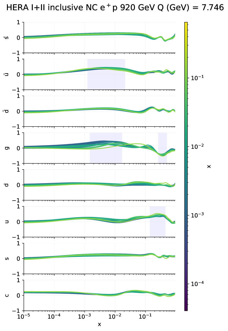
Figure 25: The correlation coefficient $\rho$ Eq. (33) between the closure test PDFs of the $\lambda=1$ set of Sect. 3.2, and the neutral-current deep-inelastic reduced cross-section $,{\cal O}=\sigma_{\rm NC}^{e^{+}p}(x,Q^{2})$. The correlation coefficient is plotted vs. the $x$ value of the PDF for PDFs at the parametrisation scale $Q_{0}=1.651$ GeV. Each curve corresponds to a datapoint in the HERA I+II dataset of Tab. 1, with $Q^{2}=60$ GeV² ($E_{p}=920$ GeV data, left panel) or $10\leq Q^{2}\leq 30$ GeV² ($E_{p}=460$ GeV data, right panel) and the value of $x$ shown by the color coding. The region in which $\rho>0.7\rho_{\rm max}$ is highlighted.

In Fig. 26 we display the correlation computed using the $\lambda=1$ PDF set of Sect. 3.3, now shown for the single dataset in which the inconsistency is introduced, and for the out-of-sample dataset that is mostly affected by it, namely the ATLAS high-mass Drell-Yan measurements at $8$ and $7$ TeV respectively, also shown in Fig. 14. In this case, each curve for the $8$ TeV dataset refers to a dilepton rapidity bin, averaged over all values of the gauge boson virtuality, and for the $7$ TeV to an invariant mass bin.

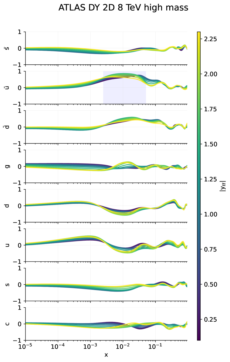
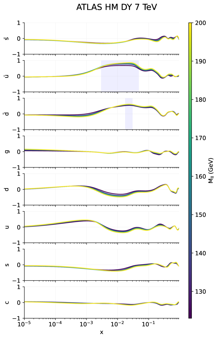
Figure 26: Same as Fig. 25, for the closure test PDFs of Sect. 3.3 and ATLAS high-mass Drell-Yan measurements at $8$ and $7$ TeV respectively. For the $8$ TeV dataset (left) each curve refers to a dilepton rapidity bin, averaged over all values of the gauge boson virtuality, and for the $7$ TeV dataset (right) to an invariant mass bin.

We finally show in Fig. 27 the correlations for the closure test PDFs of Sect. 3.4, also in this case for the dataset in which the inconsistency is introduced, and for the out-of-sample dataset that is mostly affected by it, namely respectively ATLAS single-inclusive jets and the CMS $t\bar{t}$ double differential cross section at $8$ TeV.

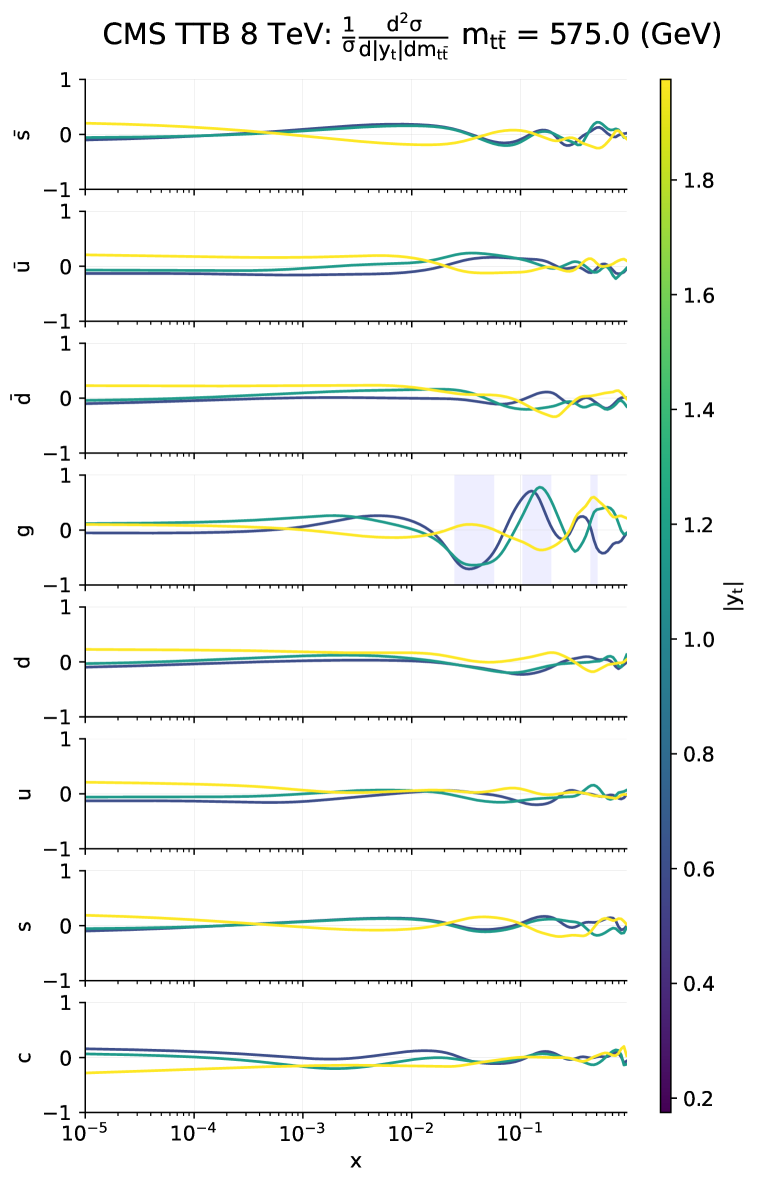
Figure 27: Same as Fig. 25, for the closure test PDFs of Sect. 3.4 and ATLAS single-inclusive jets (left) and CMS $t\bar{t}$ double differential cross section at $8$ TeV (right), with individual curves corresponding to fixed $k_{T}$ in the former case, and to fixed top rapidity averaged over top pair invariant mass in the latter case.

References

- (1) S. Amoroso et al., Snowmass 2021 Whitepaper: Proton Structure at the Precision Frontier, Acta Phys. Polon. B 53 (2022), no. 12 12–A1, [arXiv:2203.13923].
- (2) M. Ubiali, Parton Distribution Functions and Their Impact on Precision of the Current Theory Calculations, 4, 2024. arXiv:2404.08508.
- (3) D. Guest, K. Cranmer, and D. Whiteson, Deep Learning and its Application to LHC Physics, Ann. Rev. Nucl. Part. Sci. 68 (2018) 161–181, [arXiv:1806.11484].
- (4) K. Albertsson et al., Machine Learning in High Energy Physics Community White Paper, J. Phys. Conf. Ser. 1085 (2018), no. 2 022008, [arXiv:1807.02876].
- (5) T. Plehn, A. Butter, B. Dillon, T. Heimel, C. Krause, and R. Winterhalder, Modern Machine Learning for LHC Physicists, arXiv:2211.01421.
- (6) NNPDF Collaboration, R. D. Ball et al., Parton distributions for the LHC Run II, JHEP 04 (2015) 040, [arXiv:1410.8849].
- (7) L. Demortier, Proceedings, PHYSTAT 2011 Workshop on Statistical Issues Related to Discovery Claims in Search Experiments and Unfolding, CERN,Geneva, Switzerland 17-20 January 2011, ch. Open Issues in the Wake of Banff 2011. 2011.
- (8) G. Watt and R. S. Thorne, Study of Monte Carlo approach to experimental uncertainty propagation with MSTW 2008 PDFs, JHEP 1208 (2012) 052, [arXiv:1205.4024].
- (9) L. Del Debbio, T. Giani, and M. Wilson, Bayesian approach to inverse problems: an application to NNPDF closure testing, Eur. Phys. J. C 82 (2022), no. 4 330, [arXiv:2111.05787].
- (10) L. A. Harland-Lang, T. Cridge, and R. S. Thorne, A Stress Test of Global PDF Fits: Closure Testing the MSHT PDFs and a First Direct Comparison to the Neural Net Approach, arXiv:2407.07944.
- (11) E. Hammou, Z. Kassabov, M. Madigan, M. L. Mangano, L. Mantani, J. Moore, M. M. Alvarado, and M. Ubiali, Hide and seek: how PDFs can conceal new physics, JHEP 11 (2023) 090, [arXiv:2307.10370].
- (12) M. N. Costantini, E. Hammou, Z. Kassabov, M. Madigan, L. Mantani, M. Morales Alvarado, J. M. Moore, and M. Ubiali, SIMUnet: an open-source tool for simultaneous global fits of EFT Wilson coefficients and PDFs, arXiv:2402.03308.
- (13) E. Hammou and M. Ubiali, Unravelling New Physics Signals at the HL-LHC with Low-Energy Constraints, arXiv:2410.00963.
- (14) NNPDF Collaboration, R. D. Ball et al., The path to proton structure at 1% accuracy, Eur. Phys. J. C 82 (2022), no. 5 428, [arXiv:2109.02653].
- (15) P. Hall, The bootstrap and edgeworth expansion, 1992.
- (16) M. N. Costantini, M. Madigan, L. Mantani, and J. M. Moore, A critical study of the Monte Carlo replica method, arXiv:2404.10056.
- (17) S. Carrazza, S. Forte, Z. Kassabov, J. I. Latorre, and J. Rojo, An Unbiased Hessian Representation for Monte Carlo PDFs, Eur. Phys. J. C75 (2015), no. 8 369, [arXiv:1505.06736].
- (18) PDF4LHC Working Group Collaboration, R. D. Ball et al., The PDF4LHC21 combination of global PDF fits for the LHC Run III, J. Phys. G 49 (2022), no. 8 080501, [arXiv:2203.05506].
- (19) S. Carrazza, J. I. Latorre, J. Rojo, and G. Watt, A compression algorithm for the combination of PDF sets, Eur. Phys. J. C75 (2015) 474, [arXiv:1504.06469].
- (20) S. Carrazza, S. Forte, Z. Kassabov, and J. Rojo, Specialized minimal PDFs for optimized LHC calculations, Eur. Phys. J. C76 (2016), no. 4 205, [arXiv:1602.00005].
- (21) S. Forte, Parton distributions at the dawn of the LHC, Acta Phys.Polon. B41 (2010) 2859, [arXiv:1011.5247].
- (22) NNPDF Collaboration, R. D. Ball et al., An open-source machine learning framework for global analyses of parton distributions, Eur. Phys. J. C 81 (2021), no. 10 958, [arXiv:2109.02671].
- (23) New Muon Collaboration, M. Arneodo et al., Accurate measurement of and , Nucl. Phys. B487 (1997) 3–26, [hep-ex/9611022].
- (24) L. W. Whitlow, E. M. Riordan, S. Dasu, S. Rock, and A. Bodek, Precise measurements of the proton and deuteron structure functions from a global analysis of the SLAC deep inelastic electron scattering cross-sections, Phys. Lett. B282 (1992) 475–482.
- (25) BCDMS Collaboration, A. C. Benvenuti et al., A High Statistics Measurement of the Proton Structure Functions and from Deep Inelastic Muon Scattering at High , Phys. Lett. B223 (1989) 485.
- (26) CHORUS Collaboration, G. Onengut et al., Measurement of nucleon structure functions in neutrino scattering, Phys. Lett. B632 (2006) 65–75.
- (27) NuTeV Collaboration, M. Goncharov et al., Precise measurement of dimuon production cross-sections in Fe and Fe deep inelastic scattering at the Tevatron, Phys. Rev. D64 (2001) 112006, [hep-ex/0102049].
- (28) D. A. Mason, Measurement of the strange - antistrange asymmetry at NLO in QCD from NuTeV dimuon data, . FERMILAB-THESIS-2006-01.
- (29) ZEUS, H1 Collaboration, H. Abramowicz et al., Combination of measurements of inclusive deep inelastic scattering cross sections and QCD analysis of HERA data, Eur. Phys. J. C75 (2015), no. 12 580, [arXiv:1506.06042].
- (30) H1, ZEUS Collaboration, H. Abramowicz et al., Combination and QCD analysis of charm and beauty production cross-section measurements in deep inelastic scattering at HERA, Eur. Phys. J. C78 (2018), no. 6 473, [arXiv:1804.01019].
- (31) New Muon Collaboration, M. Arneodo et al., Measurement of the proton and deuteron structure functions, and , and of the ratio , Nucl. Phys. B483 (1997) 3–43, [hep-ph/9610231].
- (32) ATLAS Collaboration, G. Aad et al., Measurement of the double-differential high-mass Drell-Yan cross section in pp collisions at TeV with the ATLAS detector, JHEP 08 (2016) 009, [arXiv:1606.01736].
- (33) ATLAS Collaboration, Measurement of the double-differential high-mass drell-yan cross section in pp collisions at s = 8 tev with the atlas detector, Journal of High Energy Physics 2016 (Aug., 2016).
- (34) LHCb Collaboration, R. Aaij et al., Measurement of the forward boson production cross-section in collisions at TeV, JHEP 08 (2015) 039, [arXiv:1505.07024].
- (35) LHCb Collaboration, R. Aaij et al., Measurement of the forward Z boson production cross-section in pp collisions at TeV, JHEP 09 (2016) 136, [arXiv:1607.06495].
- (36) ATLAS Collaboration, M. Aaboud et al., Measurement of differential cross sections and cross-section ratios for boson production in association with jets at TeV with the ATLAS detector, JHEP 05 (2018) 077, [arXiv:1711.03296]. [Erratum: JHEP 10, 048 (2020)].
- (37) CMS Collaboration, S. Chatrchyan et al., Measurement of the Muon Charge Asymmetry in Inclusive Production at 7 TeV and an Improved Determination of Light Parton Distribution Functions, Phys. Rev. D 90 (2014), no. 3 032004, [arXiv:1312.6283].
- (38) ATLAS Collaboration, G. Aad et al., Measurement of the production cross-section using events with b-tagged jets in pp collisions at = 7 and 8 with the ATLAS detector, Eur. Phys. J. C 74 (2014), no. 10 3109, [arXiv:1406.5375]. [Addendum: Eur.Phys.J.C 76, 642 (2016)].
- (39) ATLAS Collaboration, G. Aad et al., Measurement of the high-mass Drell–Yan differential cross-section in pp collisions at sqrt(s)=7 TeV with the ATLAS detector, Phys. Lett. B 725 (2013) 223–242, [arXiv:1305.4192].
- (40) ATLAS Collaboration, M. Aaboud et al., Fiducial, total and differential cross-section measurements of -channel single top-quark production in collisions at 8 TeV using data collected by the ATLAS detector, Eur. Phys. J. C 77 (2017), no. 8 531, [arXiv:1702.02859].
- (41) CMS Collaboration, A. M. Sirunyan et al., Measurement of the inclusive cross section in pp collisions at TeV using final states with at least one charged lepton, JHEP 03 (2018) 115, [arXiv:1711.03143].
- (42) CMS Collaboration, A. M. Sirunyan et al., Measurement of double-differential cross sections for top quark pair production in pp collisions at TeV and impact on parton distribution functions, Eur. Phys. J. C 77 (2017), no. 7 459, [arXiv:1703.01630].
- (43) CMS Collaboration, V. Khachatryan et al., Measurement and QCD analysis of double-differential inclusive jet cross sections in pp collisions at TeV and cross section ratios to 2.76 and 7 TeV, JHEP 03 (2017) 156, [arXiv:1609.05331].
- (44) ATLAS Collaboration, M. Aaboud et al., Measurement of the inclusive jet cross-sections in proton-proton collisions at TeV with the ATLAS detector, JHEP 09 (2017) 020, [arXiv:1706.03192].
- (45) ATLAS Collaboration, M. Aaboud et al., Precision measurement and interpretation of inclusive , and production cross sections with the ATLAS detector, Eur. Phys. J. C 77 (2017), no. 6 367, [arXiv:1612.03016].
- (46) CDF Collaboration, T. A. Aaltonen et al., Measurement of of Drell-Yan pairs in the Mass Region from Collisions at TeV, Phys. Lett. B 692 (2010) 232–239, [arXiv:0908.3914].
- (47) A. Ablat et al., New results in the CTEQ-TEA global analysis of parton distributions in the nucleon, Eur. Phys. J. Plus 139 (2024), no. 12 1063, [arXiv:2408.04020].
- (48) B. Efron, Bootstrap Methods: Another Look at the Jackknife, Annals Statist. 7 (1979), no. 1 1–26.
- (49) B. Efron and R. Tibshirani, An introduction to the bootstrap, Statist. Sci. 57 (1986), no. 1 54–75.
- (50) R. D. Ball, S. Forte, and R. Stegeman, Correlation and combination of sets of parton distributions, Eur. Phys. J. C 81 (2021), no. 11 1046, [arXiv:2110.08274].