LTH 1397, P3H-25-020, TTP25-007, ZU-TH 19/25
Three-loop large-$N_{c}$ virtual corrections to $gg\to HH$ in the forward limit

Abstract

We compute the three-loop form factors for $gg\to HH$ in the limit of vanishing transverse momentum of the Higgs boson which provides a reasonable approximation of the cross section. In our calculations we adopt the large-$N_{c}$ limit, which already includes non-trivial non-planar Feynman diagrams. We discuss the results for top quark masses in the pole and $\overline{\rm MS}$ schemes and show that the scheme dependence is significantly reduced at next-to-next-to-leading order.

1 Introduction

Higgs boson pair production is one of the processes which will get a lot of attention in the upcoming years – both from the experimental and the theory side. The main production channel is via gluon fusion which shows a sizable dependence on the top quark mass. As a consequence, there is a relatively strong dependence on the top quark mass renormalization scheme as has been discussed in Refs. [1, 2]. It amounts up to 20% after including the next-to-leading order (NLO) corrections into the theory predictions. In order to reduce this uncertainty it is necessary to move to next-to-next-to-leading order (NNLO), which involves both virtual corrections to $gg\to HH$ and real radiation contributions with one or two additional massless partons in the final state.

The strong scheme dependence at NLO has its origin in the two-loop virtual corrections. The contribution which is most important for its reduction is the three-loop virtual correction to the $gg\to HH$ form factors. Here $m_{t}$ has to be renormalized at the two-loop level. Sample Feynman diagrams are shown in Figs. 1 and 2. In this paper we advance the findings of Ref. [3], where light-fermion contributions have been considered (see Fig. 1(b)) to the next step and compute the complete dependence on the top quark mass in the forward limit for vanishing transverse momenta of the Higgs bosons, albeit restricting to the contributions with one closed top quark loop and also to the large-$N_{c}$ (where $N_{c}$ stands for the number of colours in QCD) approximation, see Fig. 2(a) to (c) for sample Feynman diagrams. This allows us to estimate the reduction of the uncertainty due to the top quark mass renormalization scheme. One-particle reducible contributions as, e.g., shown in Fig. 1(a) have been computed in Ref. [4] using semi-analytic methods in the whole phase space. One-particle irreducible contributions as shown in Fig. 1(c) are not known beyond the large-$m_{t}$ limit.

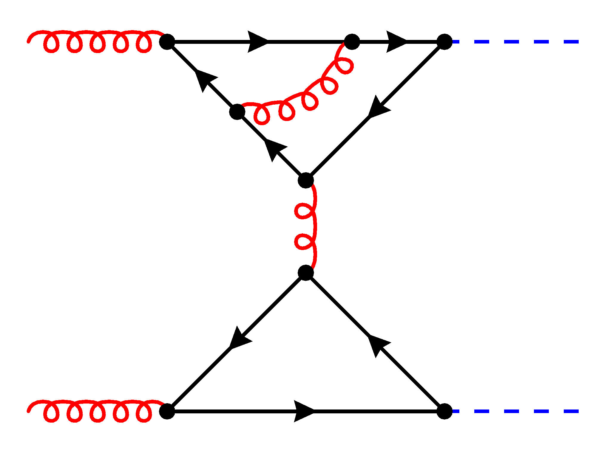
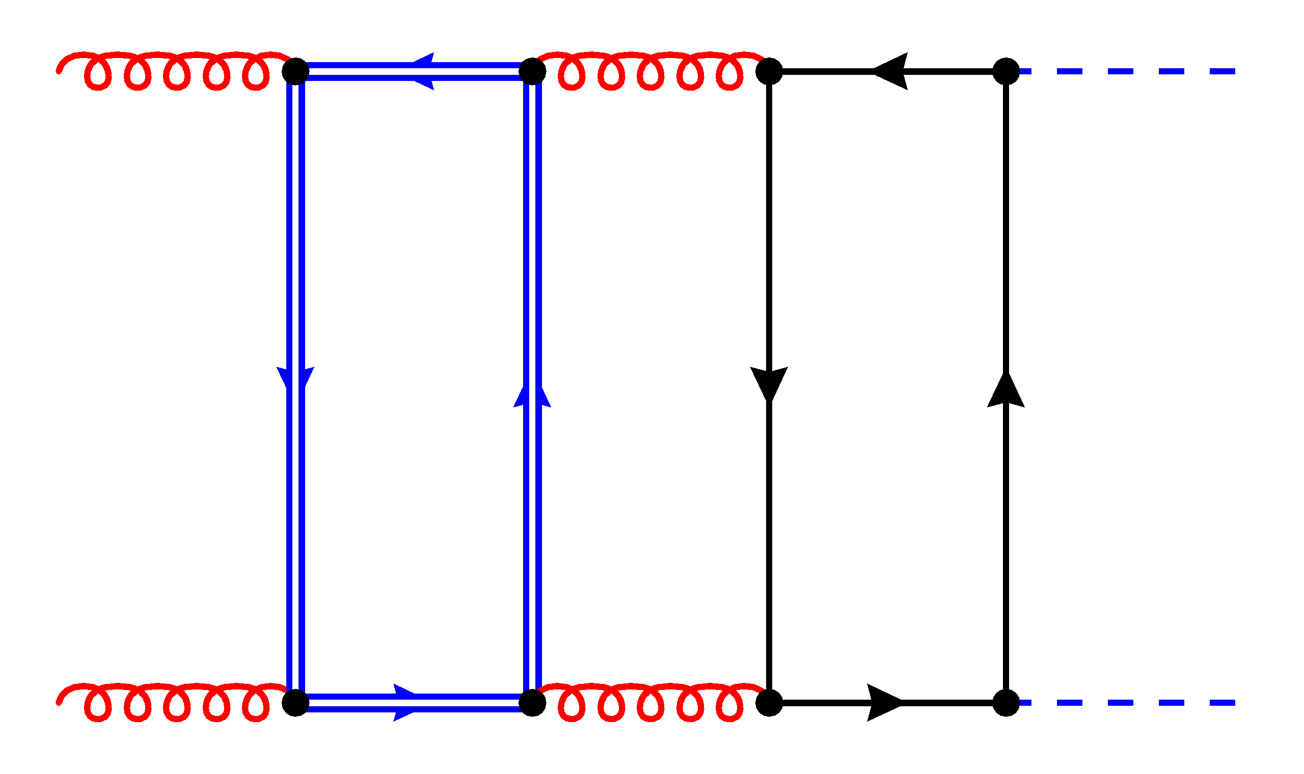
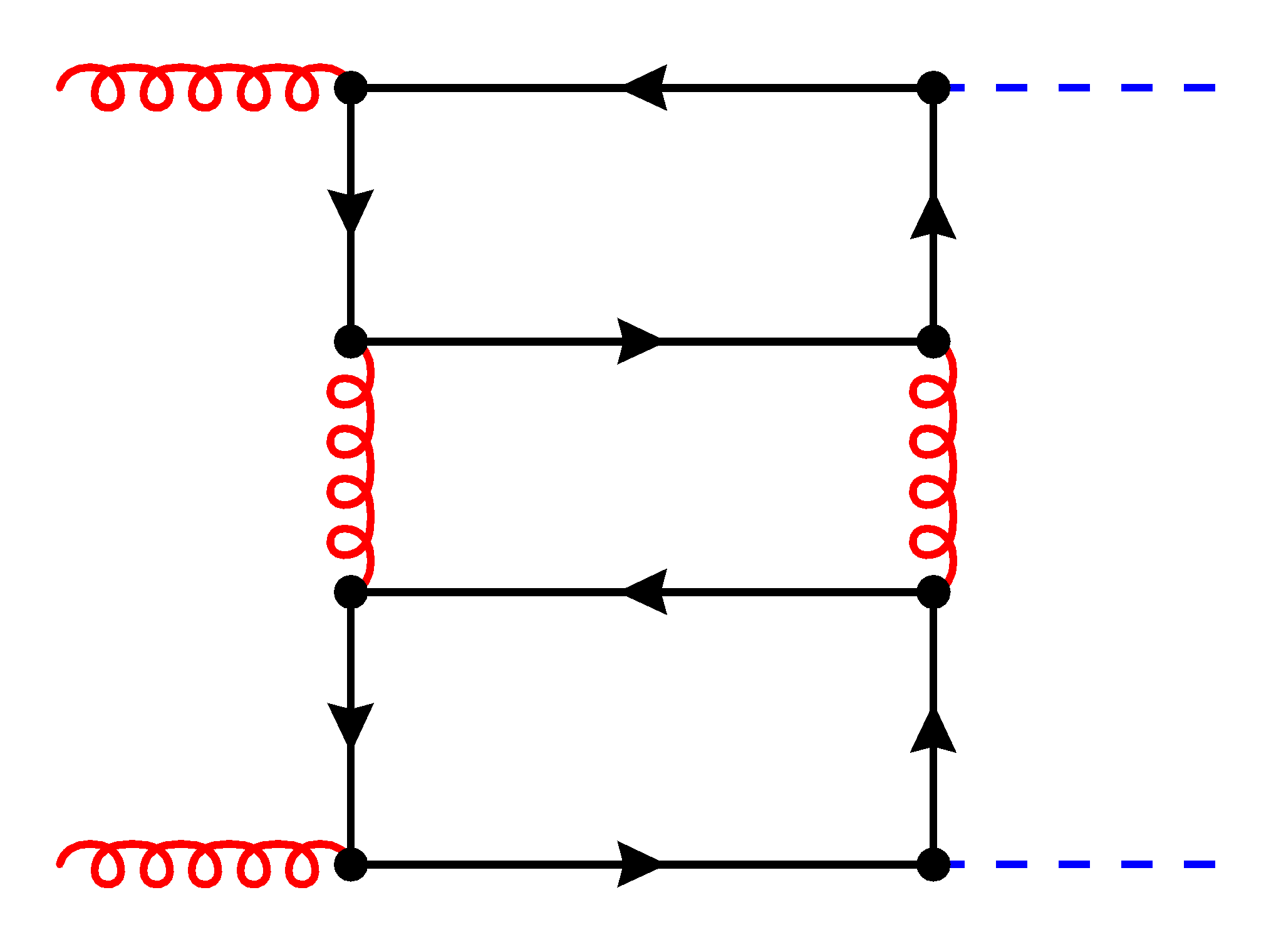
(a)                 (b)                 (c)

Figure 1: Sample Feynman diagrams of contributions which are not computed in the present paper. The contributions shown represent: (a) reducible contributions, (b) contributions with one closed light quark loop, (c) contributions with two closed top quark loops. Curly (red) lines correspond to gluons, single (black) lines to the top quark, double (blue) lines to a massless quark and dashed (blue) lines to the Higgs boson.

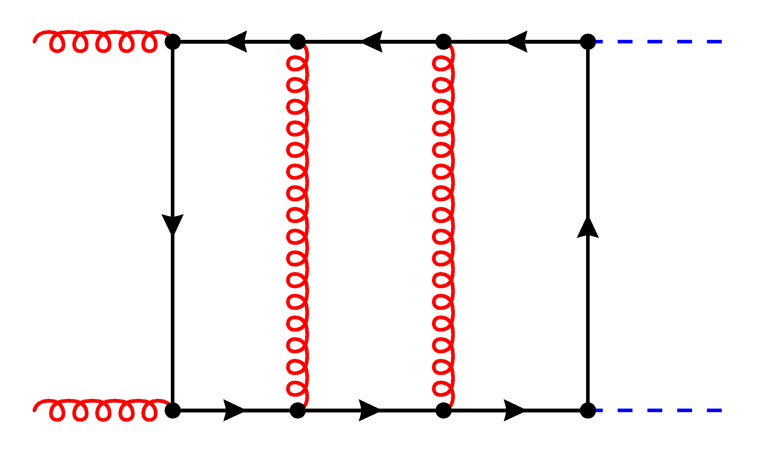
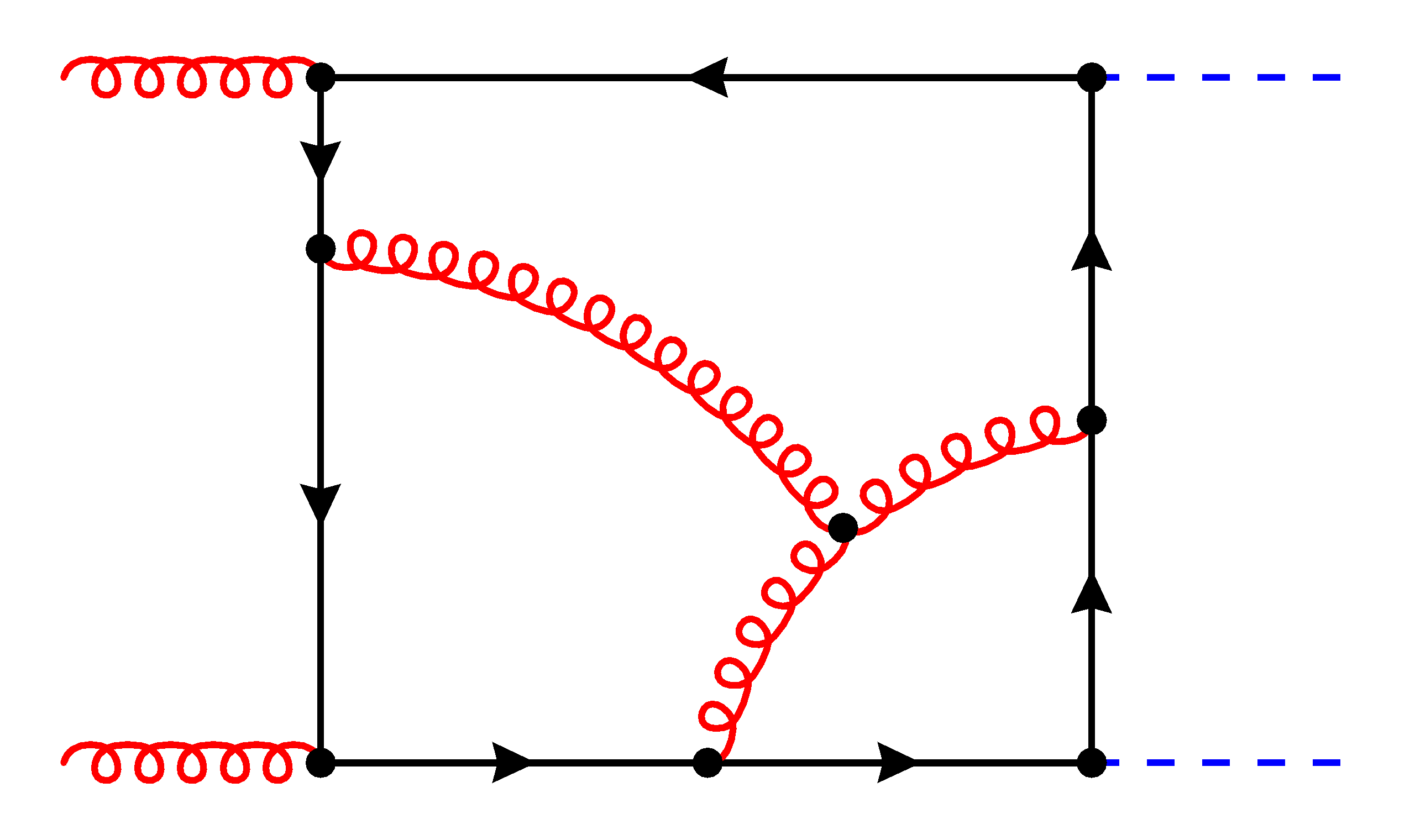
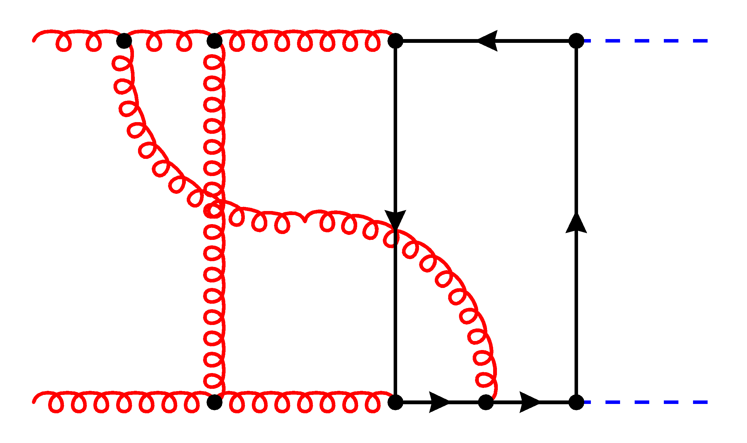
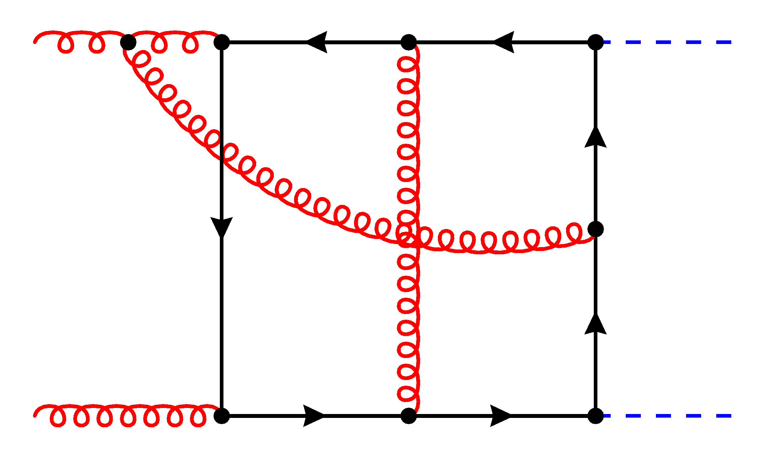
(a)            (b)            (c)            (d)

Figure 2: Sample Feynman diagrams of the contributions containing one closed top quark loop. Diagrams (a)-(c) contribute in the leading-$N_{c}$ limit, while (d) is suppressed in this limit. The line styles are as in Fig. 1.

We consider the process $g(q_{1})+g(q_{2})\to H(q_{3})+H(q_{4})$ where all momenta are incoming. Then the Mandelstam variables are given by

$$s=(q_{1}+q_{2})^{2}\,,\qquad t=(q_{1}+q_{3})^{2}\,,\qquad u=(q_{2}+q_{3})^{2}\,,$$ (1)

with $s+t+u=2m_{H}^{2}$ and the transverse momentum of the Higgs boson is given by $p_{T}^{2}=(tu-m_{H}^{4})/s$. The matrix element is conveniently decomposed into two form factors

$${\cal M}^{ab} = \varepsilon_{1,\mu}\varepsilon_{2,\nu}{\cal M}^{\mu\nu,ab}\,\,=\,\,\varepsilon_{1,\mu}\varepsilon_{2,\nu}\delta^{ab}X_{0}s\left(F_{1}A_{1}^{\mu\nu}+F_{2}A_{2}^{\mu\nu}\right)\,,$$ (2)

with

$$X_{0}(\mu) = \frac{G_{F}}{\sqrt{2}}\frac{\alpha_{s}(\mu)}{2\pi}T_{F}\,,$$ (3)

with the Fermi constant $G_{F}$, the strong coupling constant $\alpha_{s}(\mu)$ in the $\overline{\rm MS}$ scheme and $T_{F}=1/2$. At higher orders we will also need the colour factors $C_{F}=(N_{c}^{2}-1)/(2N_{c})$ and $C_{A}=N_{c}$. We introduce the perturbative expansion of $F_{1}$ and $F_{2}$ as

$$F = F^{(0)}+\left(\frac{\alpha_{s}(\mu)}{\pi}\right)F^{(1)}+\left(\frac{\alpha_{s}(\mu)}{\pi}\right)^{2}F^{(2)}+\cdots\,,$$ (4)

and decompose them into “triangle” and “box” form factors

$$F_{1}^{(k)} = \frac{3m_{H}^{2}}{s-m_{H}^{2}}F^{(k)}_{\rm tri}+F^{(k)}_{\rm box1}\,,$$

$$F_{2}^{(k)} = F^{(k)}_{\rm box2}\,.$$ (5)

Note that for $t=0$ we have $F_{2}=0$, which we have explicitly checked in our calculation. In this work we concentrate on $F^{(2)}_{\rm box1}$ since the three-loop triangle form factor has already been computed in Refs. [5, 6, 7, 8].

Leading-order predictions to $gg\to HH$ are known from Refs. [9, 10] and NLO corrections based on a purely numerical approach have been obtained in Ref. [11, 12, 13]. In Refs. [14, 15] it has been shown that the combination of deep high-energy expansions [16, 17, 15] and results from the expansion for small transverse momentum [18, 15] lead to precise results for the two-loop form factors which can be evaluated numerically in a fast and flexible way.

Predictions at NNLO and N³LO are mainly restricted to the large top quark mass limit (see, e.g. Refs. [19, 20, 21, 22, 23]) with the exception of Ref. [3] where the three-loop light-fermion contributions have been computed for $t=0$ and $m_{H}=0$ but taking into account the full dependence on $s/m_{t}^{2}$. Recently also the leading logarithmic high-energy behaviour of the form factors has been studied in Ref. [24].

The remainder of the paper is organized as follows: In the next section we present details of our calculations and discuss the various challenges. Afterwards, in Section 3 we briefly discuss the ultraviolet and infrared behaviour of the three-loop form factor. We also discuss the dependence of our form factor on the renormalization scales for the strong coupling constant and the top quark mass. We present the results for the form factors in Section 4 and discuss in particular the reduction of the scheme dependence. We conclude in Section 5 and give a brief outlook.

2 Technical details

The calculation follows the same strategy as has been outlined in Ref. [3] for the light fermion contributions. However, in order to perform the calculation for the large-$N_{c}$ contributions several improvements had to be implemented.

We generate the diagrams required for our calculation with qgraf [25], and then use tapir [26] and exp [27, 28] to map the diagrams onto topologies in full kinematics and convert the output to FORM [29] notation. The diagrams are then computed with the in-house “calc” setup, to produce an amplitude in terms of scalar Feynman integrals in a highly automated way.

Next we perform the expansions for $p_{T}\to 0$. The first step is to expand in the external Higgs mass $m_{H}$. In this work we only consider the leading term in the $p_{T}\to 0$ expansion, thus we can simply set $m_{H}=0$ and do not have to perform a non-trivial expansion as has been done, e.g., in Refs. [17, 30, 31].

The second step is to expand the amplitude in the forward-scattering limit (i.e. $t\to 0$). Although we are also currently only interested in the leading term in this limit we have to perform a non-trivial expansion due to factors of $1/t$ which are present in the Lorentz projectors of the form factors. We implement this expansion in FORM by introducing the vector $q_{\delta}=q_{1}+q_{3}$ and expand around $q_{\delta}=0$. We have that $q_{\delta}^{2}=t$ and use a tensor reduction procedure to treat numerators of $q_{\delta}$ contracted with loop momenta. After expanding the denominators they can become linearly dependent; we have to perform a partial fraction decomposition before the subsequent integration-by-parts (IBP) reduction to master integrals. We produce the necessary identities in two independent ways, with tapir and Limit [32], by specifying the kinematics $q_{3}=-q_{1}$. The amplitude is now given in terms of scalar loop integrals in forward kinematics.

The procedure outlined above results in 522 integral families which are not all independent. Our final simplification of the amplitude before IBP reduction is to find mappings between these families using feynson [33, 34], which results in an amplitude in terms of 203 independent integral families. We note here that the excellent performance of feynson was crucial to perform this step in a reasonable time.

At this point our amplitude is written in terms of around 2.6 million integrals belonging to the 203 independent families, which depend on the variables $d$ and $s/m_{t}^{2}$. We perform the IBP reduction for each family independently with Kira [35, 36]. The reduction of some non-planar integral families with rank-$5$ numerators is very computationally expensive and had to be performed on machines with up to $4$TB of RAM. After reducing each family individually we obtain reduction tables in terms of over 33 thousand master integrals, far too many to compute. The next procedure is to minimize the number of master integrals between the families to find a linearly independent basis. Due to resource constraints we were not able to simply reduce the master integrals between all families using Kira. Therefore we use the following procedure.

The first step is to use FIRE’s FindRules routine to find 1:1 maps between the 33 thousand integrals, which yields a basis of 4313 integrals. We then apply (a parallelized version of) FindRules to the full list of 2.6 million integrals of the amplitude to yield 1.3 million equivalent pairs. Applying the IBP tables to these pairs and comparing the left- and right-hand sides yields 820 thousand non-trivial relations involving 4029 of the 4313 basis integrals. Using Kira’s user_defined_system to find reduction relations for the redundant integrals yields a basis of 1647 master integrals. However, the differential system w.r.t. $s/m_{t}^{2}$ for this basis contains some unpleasant features, suggesting that this basis still contains linearly-dependent integrals; for example, it contains coupled systems between integrals from different sectors. To eliminate additional integrals from the basis we perform “test reductions” of a restricted integral list with FIRE 6.5 [37] (where we find excellent performance using the FUEL [38] interface to the FLINT [39] library for rational-polynomial simplification), and repeating the above steps using these reduction tables yields 35 thousand, 1817 and finally 1561 master integrals for which the differential system has a much improved structure (though the basis is likely still not fully minimal).

The calculation of this final set of 1561 master integrals poses a significant computational challenge, which we postpone for later study. In order to obtain first phenomenological relevant results we restrict ourselves to the leading-colour approximation, i.e. $C_{A}\to N_{c}$, $C_{F}\to N_{c}/2$. This reduces the set of necessary master integrals to 783, which we were able to tackle with the “expand and match” method [40, 41, 42]. We note that the leading-colour limit does not eliminate non-planar topologies from our amplitude, as e.g. shown in Fig. 2(c). Conceptionally the method is also able to address the calculation of the full set of master integrals, however, computational bottlenecks have to be overcome first. In Sec. 4 we comment on the quality of the large-$N_{c}$ approximation in the large-$m_{t}$ limit.

We compute the master integrals with the help of their differential equations with respect to $x=s/m_{t}^{2}$. First, we construct analytic results in the large-$m_{t}$ ($x\to 0$) limit. To achieve this we first insert an ansatz for the master integrals expanded around $x\to 0$ into the differential equation. This leads to a large system of linear equations for the expansion coefficients which we solve in terms of a small number of boundary coefficients. In order to fix these coefficients we compute the first few terms in the large-$m_{t}$ expansion explicitly. The calculation is facilitated by exp, which automates the asymptotic expansion in the limit $m_{t}^{2}\gg s$. The different regions lead to three-loop vacuum integrals, as well as products of one- and two-loop vacuum integrals with two- and one-loop massless $s$-channel vertex integrals, respectively, which are all well known in the literature. We only need about half of the computed expansion terms to fix the boundary conditions of our symbolic expansion; the rest are used for welcome consistency checks of our calculation. After inserting the master integrals into the amplitude we reproduce the results of Ref. [43] after specifying to the large-$N_{c}$ limit.

In a subsequent step we use the “expand and match” method to transport the results valid around $s/m_{t}^{2}\to 0$, and numerical evaluations at other points, to nearby values [40, 41, 42]. Compared to the calculation in Ref. [3] this step is much more complex; the system of equations is much larger, and exhibits various unphysical singularities in $x$ which limit the radii of convergence of the expansions. We therefore had to perform expansions around a much larger number of points:

$$\frac{s}{m_{t}^{2}} = x\in\left\{0,1,2,3,\frac{7}{2},4,\frac{9}{2},5,6,7,8,10,12,14,15,16,18,22,27,35,45\right\}~.$$ (6)

We use AMFlow [44, 45, 46, 47] at the values $x=\{1,5,10,27\}$ with 40 digits accuracy and match them directly to symbolic expansions around these points. Expansions around other points are obtained by the “expand and match” method. We verify that the expansions obtained after crossing the physical cuts at $x=4$ (the two-particle threshold) and $x=16$ (the four-particle threshold), numerically agree with at least 10 significant digits with the ones obtained from expansions obtained by matching with AMFlow runs above the cuts. This provides a strong check on the analytic continuation over these singular points of the differential equation and on the quality of the semi-numerical solutions over the whole range of $x$.

The AMFlow runs have been facilitated by the use of Symbolica [48] instead of Fermat [49] as the back-end of a modified version of Kira to perform the simplification of rational polynomials. This modification reduces the run time for a numerical evaluation of the most complicated integral families from over one month to less than a week, with similar computing resources. Using this approach we obtain smooth transitions between the different expansions with an agreement of ten or more digits at the matching points. The results provide us an accuracy of about 10 significant digits for the finite part of the form factor for $\sqrt{s}\lesssim 1000$ GeV. If required an extension to higher energies is possible.

3 Form factors in the $\overline{\rm MS}$ and pole scheme

Ultraviolet renormalization

We first renormalize the top quark mass in the pole ($M_{t}$) or $\overline{\rm MS}$ ($\overline{m}_{t}$) scheme and the strong coupling constant in the $\overline{\rm MS}$ scheme with six active flavours. This requires that we renormalize the gluon wave function for which we also use the pole scheme, i.e. the gluon two-point function with external momentum squared evaluated to zero. All counterterms are needed to two-loop order. For completeness we provide the explicit expressions (see, e.g., Refs. [50, 51, 52]):

$$Z_{m_{t}}^{\rm OS} = 1+\left(\frac{\alpha_{s}^{(6)}(\mu)}{\pi}\right)C_{F}\biggl{\{}-\frac{3}{4\epsilon}-\frac{3}{4}l_{\rm OS}-1+\epsilon\biggl{[}-\frac{3l_{\rm OS}^{2}}{8}-l_{\rm OS}-2-\frac{\pi^{2}}{16}\biggr{]}$$

$$+\epsilon^{2}\biggl{[}-\frac{l_{\rm OS}^{3}}{8}-\frac{l_{\rm OS}^{2}}{2}-\frac{1}{16}l_{\rm OS}\bigg{(}32+\pi^{2}\bigg{)}-4-\frac{\pi^{2}}{12}+\frac{\zeta_{3}}{4}\biggr{]}\biggr{\}}$$

$$+\left(\frac{\alpha_{s}^{(6)}(\mu)}{\pi}\right)^{2}\biggl{\{}\frac{1}{\epsilon^{2}}\biggl{[}\frac{11C_{A}C_{F}}{32}+\frac{9C_{F}^{2}}{32}-\frac{1}{8}C_{F}(n_{h}+n_{l})T_{F}\biggr{]}+\frac{1}{\epsilon}\biggl{[}-\frac{97}{192}C_{A}C_{F}$$

$$+\frac{9}{64}(5+4l_{\rm OS})C_{F}^{2}+\frac{5}{48}C_{F}(n_{h}+n_{l})T_{F}\biggr{]}+C_{F}T_{F}n_{l}\biggl{[}\frac{l_{\rm OS}^{2}}{8}+\frac{13l_{\rm OS}}{24}+\frac{71}{96}+\frac{\pi^{2}}{12}\biggr{]}$$

$$+C_{F}T_{F}n_{h}\biggl{[}\frac{l_{\rm OS}^{2}}{8}+\frac{13l_{\rm OS}}{24}+\frac{143}{96}-\frac{1}{6}\pi^{2}\biggr{]}+C_{F}^{2}\biggl{[}\frac{9l_{\rm OS}^{2}}{16}+\frac{45l_{\rm OS}}{32}+\frac{199}{128}-\frac{17\pi^{2}}{64}$$

$$+\frac{1}{2}\pi^{2}\log(2)-\frac{3\zeta_{3}}{4}\biggr{]}+C_{A}C_{F}\biggl{[}-\frac{11l_{\rm OS}^{2}}{32}-\frac{185l_{\rm OS}}{96}-\frac{1111}{384}+\frac{\pi^{2}}{12}$$

$$-\frac{1}{4}\pi^{2}\log(2)+\frac{3\zeta_{3}}{8}\biggr{]}\biggr{\}}\,,$$

$$Z_{m_{t}}^{\overline{\rm MS}} = 1-\frac{3C_{F}}{4\epsilon}\left(\frac{\alpha_{s}^{(6)}(\mu)}{\pi}\right)+\left(\frac{\alpha_{s}^{(6)}(\mu)}{\pi}\right)^{2}\biggl{\{}\frac{1}{\epsilon^{2}}\biggl{[}\frac{11C_{A}C_{F}}{32}+\frac{9C_{F}^{2}}{32}-\frac{1}{8}C_{F}(n_{h}+n_{l})T_{F}\biggr{]}$$

$$+\frac{1}{\epsilon}\biggl{[}-\frac{97}{192}C_{A}C_{F}-\frac{3C_{F}^{2}}{64}+\frac{5}{48}C_{F}(n_{h}+n_{l})T_{F}\biggr{]}\biggr{\}}\,,$$

$$Z_{\alpha_{s}}^{\overline{\rm MS}} = 1+\left(\frac{\alpha_{s}^{(6)}(\mu)}{\pi}\right)\frac{1}{\epsilon}\biggl{\{}-\frac{11C_{A}}{12}+\frac{T_{F}}{3}(n_{h}+n_{l})\biggr{\}}+\left(\frac{\alpha_{s}^{(6)}(\mu)}{\pi}\right)^{2}\biggl{\{}\frac{1}{\epsilon^{2}}\biggl{[}\frac{T_{F}^{2}(n_{h}+n_{l})^{2}}{9}$$

$$+\frac{121C_{A}^{2}}{144}-\frac{11}{18}C_{A}T_{F}(n_{h}+n_{l})\biggr{]}+\frac{1}{\epsilon}\biggl{[}T_{F}(n_{h}+n_{l})\biggl{(}\frac{5C_{A}}{24}+\frac{C_{F}}{8}\biggr{)}-\frac{17C_{A}^{2}}{48}\biggr{]}\biggr{\}}\,,$$

$$Z_{3}^{\rm OS} = 1+\left(\frac{\alpha_{s}^{(6)}(\mu)}{\pi}\right)T_{F}{n_{h}}\biggl{\{}-\frac{1}{3\epsilon}-\frac{l_{\rm\overline{\rm MS}}}{3}-\epsilon\left[\frac{l_{\rm\overline{\rm MS}}^{2}}{6}+\frac{\pi^{2}}{36}\right]+\epsilon^{2}\left[-\frac{l_{\rm\overline{\rm MS}}^{3}}{18}-\frac{\pi^{2}l_{\rm\overline{\rm MS}}}{36}+\frac{\zeta_{3}}{9}\right]\biggr{\}}$$ (7)

$$+\left(\frac{\alpha_{s}^{(6)}(\mu)}{\pi}\right)^{2}T_{F}{n_{h}}\Biggl{\{}\frac{1}{\epsilon^{2}}\left[\frac{35C_{F}}{144}-\frac{T_{F}n_{l}}{9}\right]+\frac{1}{\epsilon}\biggl{[}C_{A}\frac{{13}l_{\rm\overline{\rm MS}}}{72}+T_{F}{(n_{h}-n_{l})}\frac{l_{\rm\overline{\rm MS}}}{9}$$

$$-\frac{5C_{A}}{32}-\frac{C_{F}}{8}\biggr{]}+T_{F}{n_{h}}\bigg{(}\frac{l_{\rm\overline{\rm MS}}^{2}}{6}+\frac{\pi^{2}}{108}\bigg{)}-T_{F}n_{l}\bigg{(}\frac{l_{\rm\overline{\rm MS}}^{2}}{18}+\frac{\pi^{2}}{108}\bigg{)}+C_{A}\bigg{(}\frac{l_{\rm\overline{\rm MS}}^{2}}{36}-\frac{5l_{\rm\overline{\rm MS}}}{16}$$

$$+\frac{13}{192}+\frac{13\pi^{2}}{864}\bigg{)}+C_{F}\bigg{(}\frac{l_{\rm\overline{\rm MS}}}{4}-\frac{13}{48}\bigg{)}\Biggr{\}}\,,$$

with $l_{\rm\overline{\rm MS}}=\log(\mu^{2}/\overline{m}_{t}^{2})$ and $l_{\rm OS}=\log(\mu^{2}/M_{t}^{2})$. The two-loop $gg\to HH$ amplitude develops $1/\epsilon^{2}$ poles which is why we need the one-loop expressions of $Z_{m_{t}}^{\rm OS}$ and $Z_{3}^{\rm OS}$ to order $\epsilon^{2}$. The one-loop $gg\to HH$ amplitude is finite and thus constant terms in $\epsilon$ are sufficient at order $\alpha_{s}^{2}$.

We next decouple the contribution of the top quark from the running of $\alpha_{s}$ and express our amplitude in terms of $\alpha_{s}^{(5)}(\mu_{s})$. The corresponding decoupling constant defined via

$$\alpha_{s}^{(5)}(\mu_{s}) = \alpha_{s}^{(6)}(\mu_{s})\>\zeta_{\alpha_{s}}\,,$$ (8)

is given by

$$\zeta_{\alpha_{s}}^{\rm OS} = 1+\left(\frac{\alpha_{s}^{(5)}(\mu)}{\pi}\right)T_{F}{n_{h}}\left[\frac{l_{\rm OS}}{3}+\epsilon\left(\frac{l_{\rm OS}^{2}}{6}+\frac{\pi^{2}}{36}\right)+\epsilon^{2}\left(\frac{l_{\rm OS}^{3}}{18}+\frac{\pi^{2}l_{\rm OS}}{36}-\frac{\zeta_{3}}{9}\right)\right]$$ (9)

$$+\left(\frac{\alpha_{s}^{(5)}(\mu)}{\pi}\right)^{2}{T_{F}n_{h}}\left[C_{F}\left(\frac{15}{16}+\frac{l_{\rm OS}}{4}\right)+C_{A}\left(-\frac{2}{9}+\frac{5l_{\rm OS}}{12}\right)+T_{F}n_{h}\frac{l_{\rm OS}^{2}}{9}\right]\,.$$

The one-loop expression again needs to include $\epsilon^{2}$ terms. The quantity $\zeta_{\alpha_{s}}^{\overline{\rm MS}}$ is obtained with the help of the renormalization constants in Eq. (7).

Infrared subtraction

For the subtraction of the infrared poles we adapt the same procedure as in Ref. [43] which is based on Ref. [53], see also Refs. [54, 20].

Finite form factors at NLO and NNLO are obtained via the following subtraction procedure

$$F^{(1),\rm fin} = F^{(1)}-\frac{1}{2}I^{(1)}_{g}F^{(0)}\,,$$

$$F^{(2),\rm fin} = F^{(2)}-\frac{1}{2}I^{(1)}_{g}F^{(1)}-\frac{1}{4}I^{(2)}_{g}F^{(0)}\,,$$ (10)

where the quantities on the right-hand side are ultraviolet-renormalized and $I^{(1)}_{g}$ and $I^{(2)}_{g}$ are given by [53, 54]

$$I^{(1)}_{g} = {}-\left(\frac{\mu^{2}}{-s-i\delta}\right)^{\epsilon}\frac{e^{\epsilon\gamma_{E}}}{\Gamma(1-\epsilon)}\frac{1}{\epsilon^{2}}\Big{[}C_{A}+2\epsilon\beta_{0}\Big{]}\,,$$ (11)

$$I^{(2)}_{g} = {}-\left(\frac{\mu^{2}}{-s-i\delta}\right)^{2\epsilon}\left(\frac{e^{\epsilon\gamma_{E}}}{\Gamma(1-\epsilon)}\right)^{2}\frac{1}{\epsilon^{4}}\Big{[}\frac{1}{2}(C_{A}+2\epsilon\beta_{0})^{2}\Big{]}$$ (12)

$${}+\left(\frac{\mu^{2}}{-s-i\delta}\right)^{\epsilon}\frac{e^{\epsilon\gamma_{E}}}{\Gamma(1-\epsilon)}\frac{1}{\epsilon^{3}}\Big{[}2(C_{A}+2\epsilon\beta_{0})\beta_{0}\Big{]}$$

$${}-\left(\frac{\mu^{2}}{-s-i\delta}\right)^{2\epsilon}\frac{e^{\epsilon\gamma_{E}}}{\Gamma(1-\epsilon)}\bigg{\{}\frac{1}{\epsilon^{3}}\Big{[}\frac{1}{2}(C_{A}+4\epsilon\beta_{0})\beta_{0}\Big{]}$$

$$\hskip 56.9055pt-\frac{1}{\epsilon^{2}}\Big{[}\frac{(3\pi^{2}-67)C_{A}+10n_{l}}{72}(C_{A}+4\epsilon\beta_{0})\Big{]}-\frac{1}{\epsilon}\Big{[}\frac{1}{2}H_{g}\Big{]}\bigg{\}}\,,$$

with

$$\beta_{0} = \frac{1}{4}\left(\frac{11}{3}C_{A}-\frac{4}{3}Tn_{l}\right)\,,$$

$$H_{g} = C_{A}^{2}\left(\frac{\zeta_{3}}{2}+\frac{5}{12}+\frac{11\pi^{2}}{144}\right)+C_{A}n_{l}\left(\frac{29}{27}+\frac{\pi^{2}}{72}\right)+\frac{1}{2}C_{F}n_{l}+\frac{5}{27}n_{l}^{2}\,.$$ (13)

We compute all counterterm contributions and infrared subtraction terms for general colour factors. Afterwards we select the leading-$N_{c}$ terms for the contributions with one closed top quark loop. Furthermore we add the light-fermion contributions (“$n_{l}$”) computed in Ref. [3]. The renormalization and infrared subtraction procedure also produces $n_{l}^{2}$ terms, which we take into account. These (which are numerically small even for $n_{l}=5$) cancel against the convolutions with splitting functions which are part of the real radiation contribution.

Renormalization scales

Note that the subtraction terms in Eq. (12) are chosen in such a way that the renormalization scale dependence of $F^{\rm fin}$ is governed by $\alpha_{s}\equiv\alpha_{s}(\mu_{s})$ in case the top quark mass is renormalized on-shell. If the top quark mass is renormalized in the $\overline{\rm MS}$ scheme we introduce in a first step $\overline{m}_{t}(\mu_{s})$. Afterwards we use the two-loop renormalization group equation for $\alpha_{s}$ to separate the scales and express the form factors in terms of $\alpha_{s}(\mu_{s})$ and $\overline{m}_{t}(\mu_{t})$.

Note that each time we discuss the renormalization scale dependence of the form factors we actually have to take into account the factor $\alpha_{s}$ in Eq. (3) and have to consider the combination $\alpha_{s}(\mu_{s})F(\mu_{s},\mu_{t})$. For this reason, in the next section we show results for the quantity

$$G(\mu_{s},\mu_{t}) = \frac{\alpha_{s}(\mu_{s})}{\alpha_{s}(M_{t})}F^{\rm fin}(\mu_{s},\mu_{t})\,,$$ (14)

where $M_{t}$ is the top quark pole mass.

4 Scheme and scale dependence of the form factor at NNLO

We use the same input values as in Ref. [3] which are given by

$$M_{t} = 173.21~\mbox{GeV}\,,$$

$$m_{H} = 125.10~\mbox{GeV}\,,$$

$$\alpha_{s}^{(5)}(M_{Z}) = 0.118\,.$$ (15)

For the numerical evaluation of the form factors we need $\alpha_{s}^{(5)}(\mu_{s})$ and $\overline{m}_{t}(\mu_{t})$. For the latter we also need $\alpha_{s}^{(6)}(\mu_{t})$. The corresponding numerical values are obtained using RunDec [55] with five-loop running and four-loop matching at $\mu=M_{t}$ for the transition from the $n_{f}=5$ to the $n_{f}=6$ flavour theory. For reference we provide the values for $\mu_{t}=\mu_{s}=\overline{m}_{t}(\overline{m}_{t})$:

$$\overline{m}_{t}(\overline{m}_{t}) = 163.39~\mbox{GeV}\,,$$

$$\alpha_{s}^{(6)}(\overline{m}_{t}(\overline{m}_{t})) = 0.108\,.$$ (16)

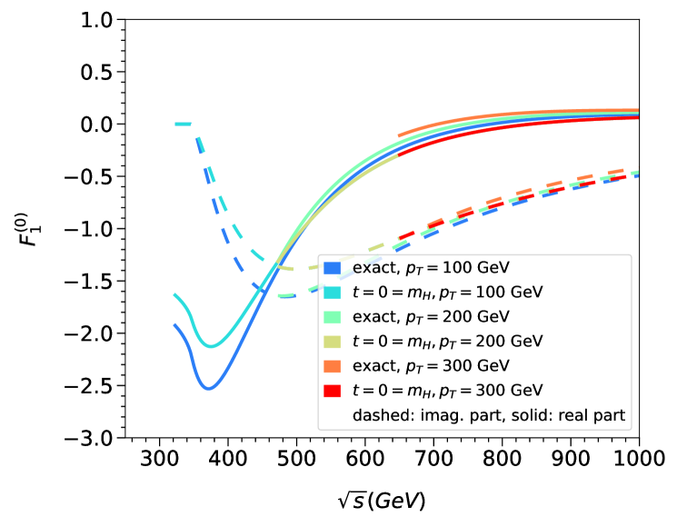
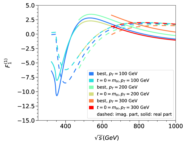
Figure 3: One- and two-loop results for $F_{1}^{\rm fin}$. We show both the exact result and the approximation for $t=0$ and $m_{H}=0$ (which does not depend on $p_{T}$) for various values of $p_{T}$. For the two-loop curves we choose $\mu^{2}=-s$ as in Ref. [3]. The label “best” refers to the combination of the small-$t$ and high-energy expansions which have been shown to be equivalent to the exact result, see Ref. [15].

We start in Fig. 3 by showing the real and imaginary parts of the one- and two-loop form factor $F_{1}^{\rm fin}$. The exact results are compared to the approximation we apply at three loops ($t=0$ and $m_{H}=0$). Note that this approximation is independent of $p_{T}$. For the exact result we show curves for $p_{T}=100$ GeV, $p_{T}=200$ GeV and $p_{T}=300$ GeV. Fig. 3 is based on data from Ref. [3] where $\mu_{s}^{2}=-s$ has been chosen and the top quark mass has been renormalized in the pole scheme.

In the range of $p_{T}$ which we consider we observe, both at one and two loops and both for the real and imaginary parts, only a mild dependence on $p_{T}$. It is impressive that the forward approximation for $m_{H}=0$ agrees well with the exact result. Around the top–anti-top threshold we observe a deviation of only 20%. This suggests that the three-loop approximation for $t=0$ and $m_{H}=0$ already provides phenomenologically relevant results, since a large part of the total cross section is provided for values of the transverse momentum around 100 GeV.

Next we discuss the quality of the large-$N_{c}$ approximation, which we can test in the large-$m_{t}$ limit where results for all colour structures are available [43]. If we concentrate on the leading $N_{c}^{2}$ term of the contribution with one closed top quark loop and consider the leading term in the $1/m_{t}$ expansion and values for $\sqrt{s}$ and $p_{T}$ where the large-$m_{t}$ approximation is valid (i.e., $250$ GeV$\lesssim\sqrt{s}\lesssim 300$ GeV and $p_{T}$ below about 50 GeV) we observe that the deviation between the full results and the leading $N_{c}^{2}$ term in the real and imaginary parts of $F_{1}^{\rm fin}$ is about 5% and 30%, respectively. After including sub-leading terms in $1/m_{t}$ the agreement improves further and reaches approximately 10% for the imaginary part. Thus, it can be expected that the major contribution is covered by the large-$N_{c}$ term in the limit $p_{T}\to 0$ computed in this paper.

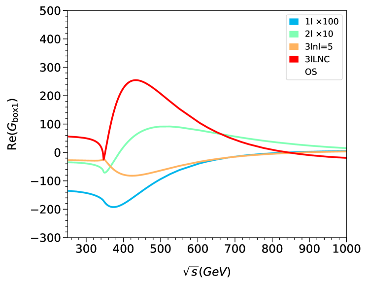
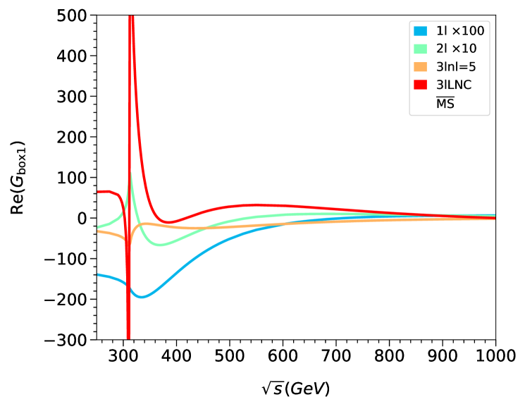
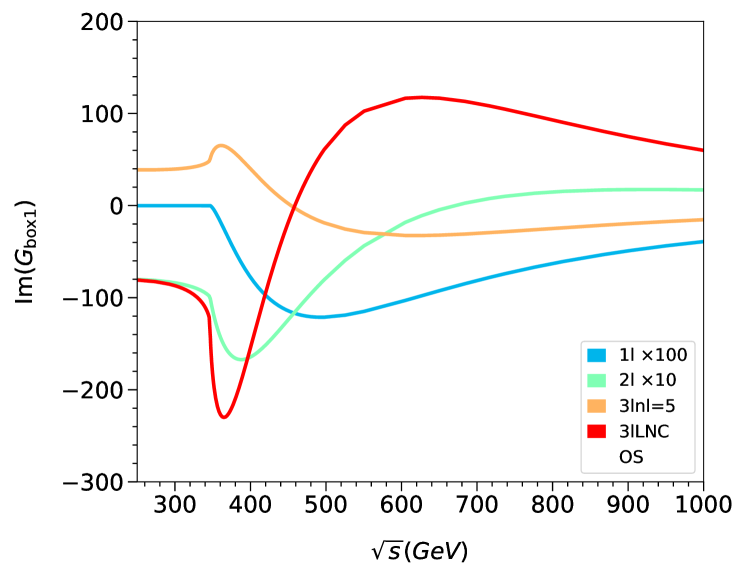
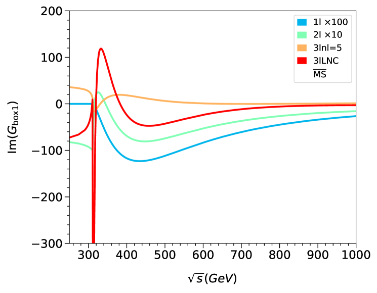
Figure 4: Real (top) and imaginary (bottom) parts of $G_{\rm box1}$ for $t=0$ and $m_{H}=0$ at one, two and three loops. The panels on the left and right use the pole and $\overline{\rm MS}$ top quark mass, respectively. At three loops the light-fermion (for $n_{l}=5$) and large-$N_{c}$ contributions are shown separately. For the renormalization scales we have chosen $\mu_{s}^{2}=\mu_{t}^{2}=s$.

In Fig. 4 we show the real and imaginary parts of the perturbative coefficients $G_{\rm box1}^{(0)}$, $G_{\rm box1}^{(1)}$ and $G_{\rm box1}^{(2)}$ (as defined in Eq. (14)) for the approximation $t=0$ and $m_{H}=0$. For the latter the light-fermion and large-$N_{c}$ results are shown separately. For the renormalization scales we have chosen $\mu_{s}^{2}=\mu_{t}^{2}=s$. For clarity the one- and two-loop results are multiplied by a factor 100 and 10, respectively. In the left-hand column the pole scheme is used for the top quark mass and on the right-hand side we use the $\overline{\rm MS}$ mass.

In the pole scheme we observe larger higher-order corrections. Depending on $\sqrt{s}$ the increase in the absolute value is in general more than an order of magnitude. This is a feature which is often observed in the pole scheme. The situation is different in the $\overline{\rm MS}$ scheme. Here the higher-order coefficients are much smaller which leads to a better convergence of perturbation theory.

The $\overline{\rm MS}$ curves show a characteristic feature around $\sqrt{s}=2\,\overline{m}_{t}\approx 320$ GeV which deserves an explanation. The top quark mass counterterm contributions from the one- and two-loop corrections are obtained via derivatives with respect to $m_{t}$. At threshold, i.e. for $s/m_{t}^{2}=4$, the derivatives are not analytic, which leads to numerically large contributions. In the pole scheme the bare three-loop form factor shows a similar behaviour with the opposite sign, such that at $s/m_{t}^{2}=4$ a smooth behaviour is observed. On the other hand, if the top quark mass is renormalized in the $\overline{\rm MS}$ scheme there is only a partial cancellation which leads to the dip-peak structure as observed in Fig. 4. Note that a similar behaviour is also observed in hadronic quantities where often bins in the Higgs boson pair invariant mass, $M_{HH}$, are used. Usually the bin including the top pair threshold shows large deviations between the $\overline{\rm MS}$ and pole scheme, see, e.g., Fig. 2 of Ref. [2]. In fact, close to threshold it is not recommended to use the $\overline{\rm MS}$ definition for the top quark mass so for practical purposes the non-physical behaviour of the form factor is not a problem.

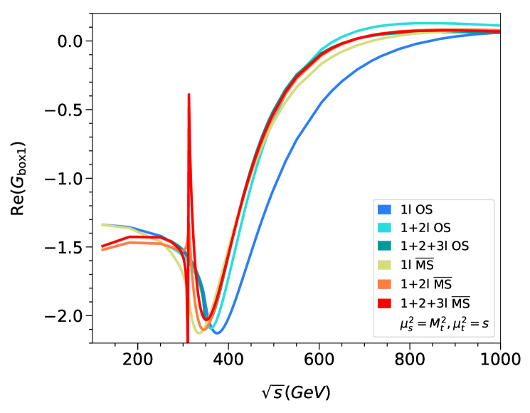
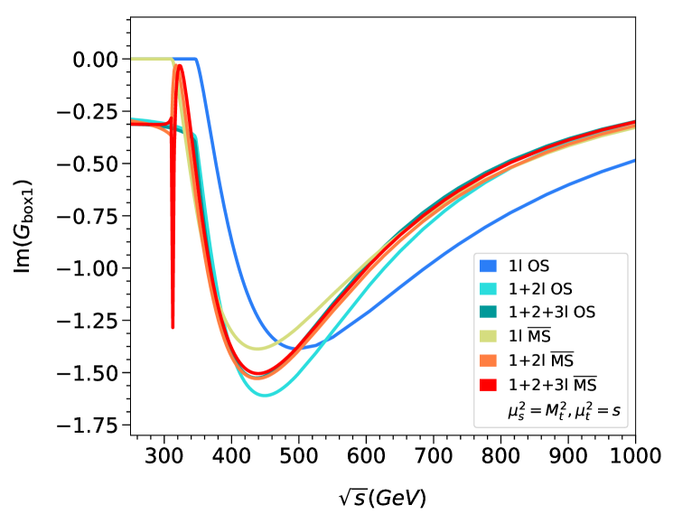
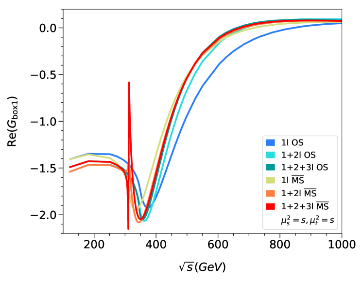
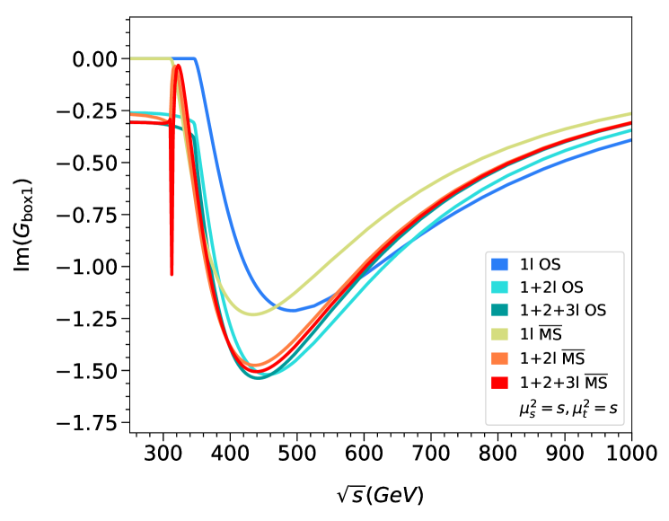
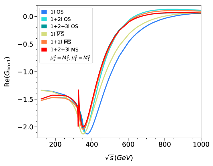
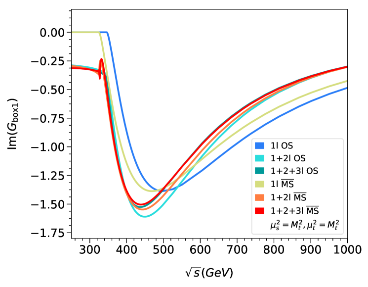
Figure 5: Real (left) and imaginary (right) parts of $F_{1}$ for $t=0$ and $m_{H}=0$. At three loops the light-fermion (for $n_{l}=5$) and large-$N_{c}$ are included. Top: $\mu_{s}^{2}={M_{t}^{2}}$, $\mu_{t}^{2}=s$, middle: $\mu_{s}^{2}=s$, $\mu_{t}^{2}=s$, bottom: $\mu_{s}^{2}={M_{t}^{2}}$, $\mu_{t}^{2}={M_{t}^{2}}$

Let us next discuss the dependence on the top quark mass scheme at NNLO. Fig. 5 shows $G_{\rm box1}$ truncated to one, two and three loops for the pole and $\overline{\rm MS}$ schemes. The real and imaginary parts are shown separately. In the different rows we adopt different choices for $\mu_{t}$ and $\mu_{s}$, namely $\mu_{s}^{2}=M_{t}^{2}$, $\mu_{t}^{2}=s$ (top), $\mu_{s}^{2}=s$, $\mu_{t}^{2}=s$ (middle) and $\mu_{s}^{2}=M_{t}^{2}$, $\mu_{t}^{2}=M_{t}^{2}$ (bottom). Due to the behaviour of the $\overline{\rm MS}$ result at $s/\overline{m}_{t}^{2}=4$ we restrict the following discussion to $\sqrt{s}\gtrsim 350$ GeV although all curves are shown also for lower values of $\sqrt{s}$.

In all cases we observe a significant reduction on the dependence of the top quark mass scheme when going from one to two and finally to three loops; the one-loop curves (blue and dark yellow) are far apart. The distance is noticeably reduced at two loops (turquoise and orange) and has almost disappeared at three loops (green and red). It is interesting to note that the orange and red curves are close together which suggests that the NNLO corrections in the $\overline{\rm MS}$ scheme are small.

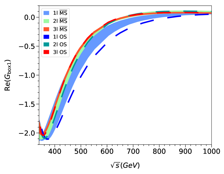
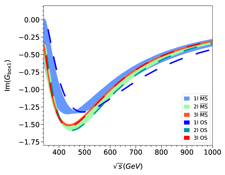
Figure 6: $G_{\rm box1}$ for $\mu_{s}^{2}=s/4$. The band is the envelope of the $\overline{\rm MS}$ result where $\mu_{t}^{2}$ is varied between $s$ and $s/16$ and $\mu_{t}^{2}={M_{t}^{2}}$ is chosen. The results in the pole scheme are shown as dashed lines. Note that at NNLO the band is quite narrow and almost completely covered by the curve from the pole scheme.

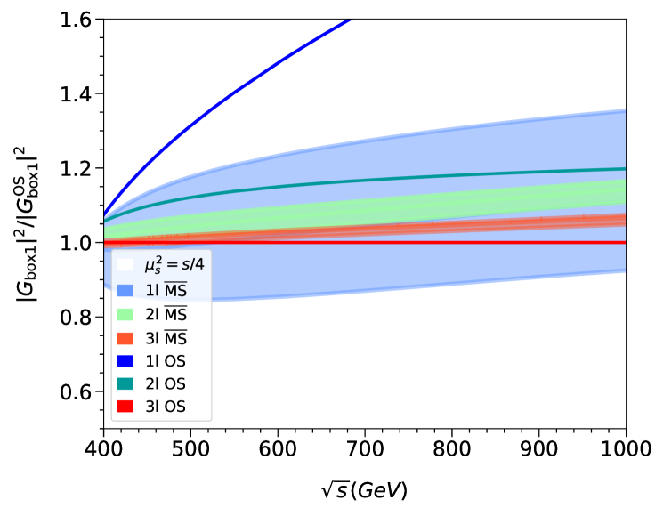
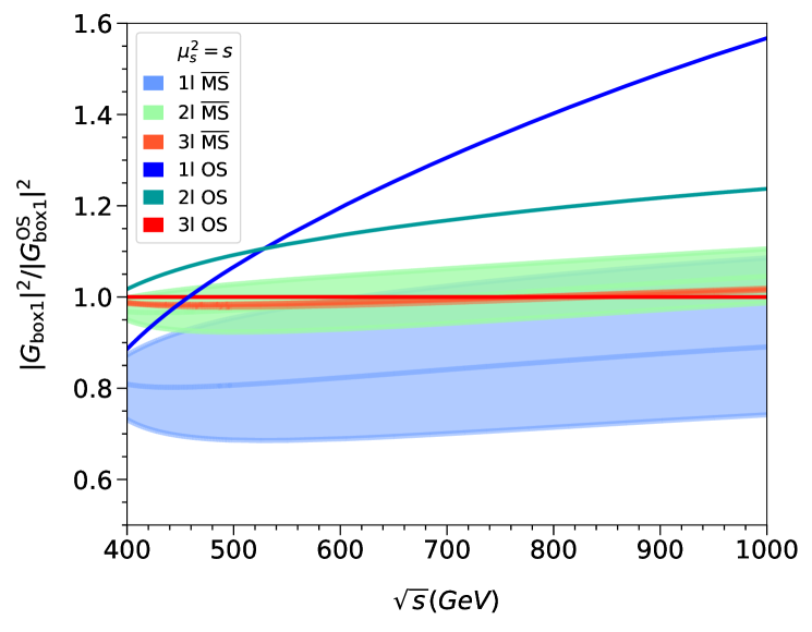
Figure 7: $G_{\rm box1}$ computed with the $\overline{\rm MS}$ and on-shell definition of the top quark mass for $\mu_{s}^{2}=s/4$ (left) and $\mu_{s}^{2}=s$ (right). $\mu_{t}^{2}$ is chosen between $s$ and $s/16$. All curves are normalized to the three-loop on-shell result.

Finally, in Fig. 6 we show $G_{\rm box1}$ in the pole and $\overline{\rm MS}$ scheme for $\sqrt{s}$ values above $340$ GeV. We choose $\mu_{s}^{2}=s/4$, and in the $\overline{\rm MS}$ scheme we vary $\mu_{t}^{2}$ between $s$ and $s/16$. This is the partonic correspondence to the often-used hadronic scale choice $\mu_{s}=M_{HH}/2$ and $\mu_{t}=M_{HH}/4,\ldots,M_{HH}$. In Fig. 6 we also include the choice $\mu_{t}^{2}=M_{t}^{2}$. For illustration the curves in the pole scheme are shown in a darker colour. The bands shown at LO, NLO and NNLO represent the envelope of the different choices of $\mu_{t}$ in the $\overline{\rm MS}$ scheme. The combination with the curves from the pole scheme reflect the uncertainty due to the scheme choice for the top quark mass.

The data used in Fig. 6 are also shown in Fig. 7 after summing the squared real and imaginary parts and normalizing to the three-loop prediction in the pole scheme. In the left panel we choose $\mu_{s}^{2}=s/4$ and the blue, green and red bands are again obtained by varying $\mu_{t}^{2}$ between $s$ and $s/16$. The LO, NLO and NNLO curves for the on-shell top quark masses are shown as dark blue, dark green and red lines, respectively. The reduction of the scale dependence is clearly seen by the smaller widths of the bands when going to higher orders in perturbation theory. Furthermore, we observe a reduction of the scheme dependence through the reduced distance between the on-shell curves and the bands which are based on $\overline{\rm MS}$ results. We observe an overlap of the NLO and NNLO bands for smaller values of $\sqrt{s}$ whereas for $\sqrt{s}\gtrsim 600$ GeV there is a small gap. Note that once also $\mu_{s}$ is varied there is an overlap of the NLO and NNLO bands. This can be seen in the right panel of Fig. 7 where $\mu_{s}^{2}=s$ has been chosen. We observe that the NNLO band is contained within the NLO scale variation.

It is interesting to note that for smaller values for $\mu_{t}$ the $\overline{\rm MS}$ curves are closer to the on-shell curves. On the other hand, in general for larger values of $\mu_{t}$ the NLO curves are more consistent with the NNLO results.

5 Conclusions and Outlook

In this paper we compute the massive three-loop box-type form factors for the process $gg\to HH$ in the large-$N_{c}$ limit for $p_{T}=0$ and massless Higgs boson in the final state. At one and two loops, we show that this limit already provides a reasonable approximation to the exact results for smaller values of $p_{T}$. We additionally consider the large-$N_{c}$ limit, which we show to provide a reasonable approximation in the context of the NNLO large-$m_{t}$ expansion.

Our calculation requires a non-trivial reduction of the box integrals to 783 master integrals. For the computation of these master integrals we apply a method which provides semi-analytic results for the desired range of $s/m_{t}^{2}$.

We use our results to study, for the first time, the scheme dependence due to the top quark mass at NNLO. We find a significant reduction, as can be seen in Fig. 6 and 7. If the scale uncertainty is estimated by the width of the bands in Fig. 7 we observe a typical reduction of about a factor five when going from NLO to NNLO. If we define the scheme uncertainty via the distance of the on-shell curves and the centre of the $\overline{\rm MS}$ band it amounts to only a few percent. For a final phenomenological analysis it is necessary to construct physical results and include the real radiation contribution in addition.

There are a few further steps necessary before a detailed phenomenological analysis is possible. These include the computation of the remaining colour coefficients, the computation of sub-leading expansion terms in $t$ and $m_{H}$, and the computation of the real-radiation contribution. Each step requires dedicated technical developments and substantial computing resources.

References

- [1] J. Baglio, F. Campanario, S. Glaus, M. Mühlleitner, J. Ronca and M. Spira, : Combined uncertainties, Phys. Rev. D 103 (2021) 056002 [2008.11626].
- [2] E. Bagnaschi, G. Degrassi and R. Gröber, Higgs boson pair production at NLO in the POWHEG approach and the top quark mass uncertainties, Eur. Phys. J. C 83 (2023) 1054 [2309.10525].
- [3] J. Davies, K. Schönwald and M. Steinhauser, Towards at next-to-next-to-leading order: Light-fermionic three-loop corrections, Phys. Lett. B 845 (2023) 138146 [2307.04796].
- [4] J. Davies, K. Schönwald, M. Steinhauser and M. Vitti, Three-loop corrections to Higgs boson pair production: reducible contribution, JHEP 08 (2024) 096 [2405.20372].
- [5] J. Davies, R. Gröber, A. Maier, T. Rauh and M. Steinhauser, Top quark mass dependence of the Higgs boson-gluon form factor at three loops, Phys. Rev. D 100 (2019) 034017 [1906.00982].
- [6] J. Davies, R. Gröber, A. Maier, T. Rauh and M. Steinhauser, Padé approach to top-quark mass effects in gluon fusion amplitudes, PoS RADCOR2019 (2019) 079 [1912.04097].
- [7] R. V. Harlander, M. Prausa and J. Usovitsch, The light-fermion contribution to the exact Higgs-gluon form factor in QCD, JHEP 10 (2019) 148 [1907.06957].
- [8] M. L. Czakon and M. Niggetiedt, Exact quark-mass dependence of the Higgs-gluon form factor at three loops in QCD, JHEP 05 (2020) 149 [2001.03008].
- [9] E. W. N. Glover and J. J. van der Bij, HIGGS BOSON PAIR PRODUCTION VIA GLUON FUSION, Nucl. Phys. B 309 (1988) 282.
- [10] T. Plehn, M. Spira and P. M. Zerwas, Pair production of neutral Higgs particles in gluon-gluon collisions, Nucl. Phys. B 479 (1996) 46 [hep-ph/9603205].
- [11] S. Borowka, N. Greiner, G. Heinrich, S. P. Jones, M. Kerner, J. Schlenk et al., Higgs Boson Pair Production in Gluon Fusion at Next-to-Leading Order with Full Top-Quark Mass Dependence, Phys. Rev. Lett. 117 (2016) 012001 [1604.06447].
- [12] S. Borowka, N. Greiner, G. Heinrich, S. P. Jones, M. Kerner, J. Schlenk et al., Full top quark mass dependence in Higgs boson pair production at NLO, JHEP 10 (2016) 107 [1608.04798].
- [13] J. Baglio, F. Campanario, S. Glaus, M. Mühlleitner, M. Spira and J. Streicher, Gluon fusion into Higgs pairs at NLO QCD and the top mass scheme, Eur. Phys. J. C 79 (2019) 459 [1811.05692].
- [14] L. Bellafronte, G. Degrassi, P. P. Giardino, R. Gröber and M. Vitti, Gluon fusion production at NLO: merging the transverse momentum and the high-energy expansions, JHEP 07 (2022) 069 [2202.12157].
- [15] J. Davies, G. Mishima, K. Schönwald and M. Steinhauser, Analytic approximations of 2 → 2 processes with massive internal particles, JHEP 06 (2023) 063 [2302.01356].
- [16] J. Davies, G. Mishima, M. Steinhauser and D. Wellmann, Double-Higgs boson production in the high-energy limit: planar master integrals, JHEP 03 (2018) 048 [1801.09696].
- [17] J. Davies, G. Mishima, M. Steinhauser and D. Wellmann, Double Higgs boson production at NLO in the high-energy limit: complete analytic results, JHEP 01 (2019) 176 [1811.05489].
- [18] R. Bonciani, G. Degrassi, P. P. Giardino and R. Gröber, Analytical Method for Next-to-Leading-Order QCD Corrections to Double-Higgs Production, Phys. Rev. Lett. 121 (2018) 162003 [1806.11564].
- [19] D. de Florian and J. Mazzitelli, Higgs Boson Pair Production at Next-to-Next-to-Leading Order in QCD, Phys. Rev. Lett. 111 (2013) 201801 [1309.6594].
- [20] J. Grigo, K. Melnikov and M. Steinhauser, Virtual corrections to Higgs boson pair production in the large top quark mass limit, Nucl. Phys. B 888 (2014) 17 [1408.2422].
- [21] M. Grazzini, G. Heinrich, S. Jones, S. Kallweit, M. Kerner, J. M. Lindert et al., Higgs boson pair production at NNLO with top quark mass effects, JHEP 05 (2018) 059 [1803.02463].
- [22] L.-B. Chen, H. T. Li, H.-S. Shao and J. Wang, Higgs boson pair production via gluon fusion at N3LO in QCD, Phys. Lett. B 803 (2020) 135292 [1909.06808].
- [23] L.-B. Chen, H. T. Li, H.-S. Shao and J. Wang, The gluon-fusion production of Higgs boson pair: N3LO QCD corrections and top-quark mass effects, JHEP 03 (2020) 072 [1912.13001].
- [24] S. Jaskiewicz, S. Jones, R. Szafron and Y. Ulrich, The structure of quark mass corrections in the amplitude at high-energy, 2501.00587.
- [25] P. Nogueira, Automatic Feynman Graph Generation, J. Comput. Phys. 105 (1993) 279.
- [26] M. Gerlach, F. Herren and M. Lang, tapir: A tool for topologies, amplitudes, partial fraction decomposition and input for reductions, Comput. Phys. Commun. 282 (2023) 108544 [2201.05618].
- [27] R. Harlander, T. Seidensticker and M. Steinhauser, Complete corrections of Order alpha alpha-s to the decay of the Z boson into bottom quarks, Phys. Lett. B 426 (1998) 125 [hep-ph/9712228].
- [28] T. Seidensticker, Automatic application of successive asymptotic expansions of Feynman diagrams, in 6th International Workshop on New Computing Techniques in Physics Research: Software Engineering, Artificial Intelligence Neural Nets, Genetic Algorithms, Symbolic Algebra, Automatic Calculation, 5, 1999, hep-ph/9905298.
- [29] B. Ruijl, T. Ueda and J. Vermaseren, FORM version 4.2, 1707.06453.
- [30] J. Davies, G. Mishima, M. Steinhauser and D. Wellmann, : analytic two-loop results for the low- and high-energy regions, JHEP 04 (2020) 024 [2002.05558].
- [31] J. Davies, K. Schönwald, M. Steinhauser and H. Zhang, Analytic next-to-leading order Yukawa and Higgs boson self-coupling corrections to at high energies, 2501.17920.
- [32] F. Herren, Precision Calculations for Higgs Boson Physics at the LHC - Four-Loop Corrections to Gluon-Fusion Processes and Higgs Boson Pair-Production at NNLO, Ph.D. thesis, KIT, Karlsruhe, 2020. 10.5445/IR/1000125521.
- [33] V. Maheria, Semi- and Fully-Inclusive Phase-Space Integrals at Four Loops, Ph.D. thesis, Hamburg U., 2022.
- [34] V. Maheria, “feynson.” https://github.com/magv/feynson.
- [35] P. Maierhöfer, J. Usovitsch and P. Uwer, Kira—A Feynman integral reduction program, Comput. Phys. Commun. 230 (2018) 99 [1705.05610].
- [36] J. Klappert, F. Lange, P. Maierhöfer and J. Usovitsch, Integral reduction with Kira 2.0 and finite field methods, Comput. Phys. Commun. 266 (2021) 108024 [2008.06494].
- [37] A. V. Smirnov and M. Zeng, FIRE 6.5: Feynman integral reduction with new simplification library, Comput. Phys. Commun. 302 (2024) 109261 [2311.02370].
- [38] K. Mokrov, A. Smirnov and M. Zeng, Rational Function Simplification for Integration-by-Parts Reduction and Beyond, 2304.13418.
- [39] The FLINT team, FLINT: Fast Library for Number Theory, 2025.
- [40] M. Fael, F. Lange, K. Schönwald and M. Steinhauser, A semi-analytic method to compute Feynman integrals applied to four-loop corrections to the -pole quark mass relation, JHEP 09 (2021) 152 [2106.05296].
- [41] M. Fael, F. Lange, K. Schönwald and M. Steinhauser, A semi-numerical method for one-scale problems applied to the -on-shell relation, SciPost Phys. Proc. 7 (2022) 041 [2110.03699].
- [42] M. Fael, F. Lange, K. Schönwald and M. Steinhauser, Singlet and nonsinglet three-loop massive form factors, Phys. Rev. D 106 (2022) 034029 [2207.00027].
- [43] J. Davies and M. Steinhauser, Three-loop form factors for Higgs boson pair production in the large top mass limit, JHEP 10 (2019) 166 [1909.01361].
- [44] X. Liu, Y.-Q. Ma and C.-Y. Wang, A Systematic and Efficient Method to Compute Multi-loop Master Integrals, Phys. Lett. B 779 (2018) 353 [1711.09572].
- [45] X. Liu and Y.-Q. Ma, Multiloop corrections for collider processes using auxiliary mass flow, Phys. Rev. D 105 (2022) L051503 [2107.01864].
- [46] Z.-F. Liu and Y.-Q. Ma, Determining Feynman Integrals with Only Input from Linear Algebra, Phys. Rev. Lett. 129 (2022) 222001 [2201.11637].
- [47] X. Liu and Y.-Q. Ma, AMFlow: A Mathematica package for Feynman integrals computation via auxiliary mass flow, Comput. Phys. Commun. 283 (2023) 108565 [2201.11669].
- [48] B. Ruijl, “Symbolica.” https://symbolica.io, Feb., 2025. 10.5281/zenodo.15040848.
- [49] R. H. Lewis, “Computer algebra system fermat.” https://home.bway.net/lewis.
- [50] N. Gray, D. J. Broadhurst, W. Grafe and K. Schilcher, Three Loop Relation of Quark (Modified) Ms and Pole Masses, Z. Phys. C 48 (1990) 673.
- [51] K. G. Chetyrkin, Four-loop renormalization of QCD: Full set of renormalization constants and anomalous dimensions, Nucl. Phys. B 710 (2005) 499 [hep-ph/0405193].
- [52] M. Gerlach, F. Herren and M. Steinhauser, Wilson coefficients for Higgs boson production and decoupling relations to , JHEP 11 (2018) 141 [1809.06787].
- [53] S. Catani, The Singular behavior of QCD amplitudes at two loop order, Phys. Lett. B 427 (1998) 161 [hep-ph/9802439].
- [54] D. de Florian and J. Mazzitelli, A next-to-next-to-leading order calculation of soft-virtual cross sections, JHEP 12 (2012) 088 [1209.0673].
- [55] F. Herren and M. Steinhauser, Version 3 of RunDec and CRunDec, Comput. Phys. Commun. 224 (2018) 333 [1703.03751].
- [56] R. V. Harlander, S. Y. Klein and M. Lipp, FeynGame, Comput. Phys. Commun. 256 (2020) 107465 [2003.00896].
- [57] R. Harlander, S. Y. Klein and M. C. Schaaf, FeynGame-2.1 – Feynman diagrams made easy, PoS EPS-HEP2023 (2024) 657 [2401.12778].
- [58] L. Bündgen, R. V. Harlander, S. Y. Klein and M. C. Schaaf, FeynGame 3.0, 2501.04651.