Euclid Quick Data Release (Q1)

The star-forming main sequence (SFMS) is a tight relation observed between stellar masses and star-formation rates (SFR) in a population of galaxies. The relation holds for different redshift, morphological, and environmental domains, and is a key to understanding the underlying relations between a galaxy budget of cold gas and its stellar content. Euclid Quick Data Release 1 (Q1) gives the opportunity to investigate this fundamental relation in galaxy formation and evolution. We complement the Euclid release with public IRAC observations of the Euclid Deep Fields (EDFs), improving the quality of recovered photometric redshifts, stellar masses, and star-formation rates, as shown both from simulations and comparison with available spectroscopic redshifts. From Q1 data alone, we recover more than $\sim 30\,\mathrm{k}$ galaxies with $\operatorname{log_{10}}(M_{\ast}/M_{\odot})>11$, giving a precise constraint of the SFMS at the high-mass end. We investigated SFMS, in a redshift interval between $0.2$ and $3.0$, comparing our results with the existing literature and fitting them with a parameterisation taking into account the presence of a bending of the relation at the high-mass end, depending on the bending mass $M_{0}$. We find good agreement with previous results in terms of $M_{0}$ values. We also investigate the distribution of physical (e.g., dust absorption $A_{V}$ and formation age) and morphological properties (e.g., Srsic index and radius) in the SFR–stellar mass plane, and their relation with the SFMS. These results highlight the potential of Euclid in studying the fundamental scaling relations that regulate galaxy formation and evolution in anticipation of the forthcoming Data Release 1.

1 Introduction

The star-forming main-sequence (SFMS) is a relation between stellar masses ($M_{\ast}$) and star-formation rates (SFRs) that is observed for star-forming galaxies (SFGs). It has been extensively studied in the last decades (Brinchmann et al. 2004; Daddi et al. 2007; Elbaz et al. 2011), investigating its slope, normalisation, scatter, and evolution over time (see Speagle et al. 2014; Popesso et al. 2023, and references therein). The SFMS is observed across different redshifts and is already in place by $z\sim 6$ (e.g., Cole et al. 2023; Clarke et al. 2024). It hosts the majority of star-formation at each epoch (Rodighiero et al. 2011), suggesting that galaxies spend most of their lifetime on the SFMS, undergoing secular evolution. The tightness of the relation, with a typical scatter of $0.3\,\mathrm{dex}$, implies its universality as the main mode of galaxy growth.

This relation emerges from the interplay between the stellar content of galaxies and their cold gas reservoirs (Schmidt 1959, i.e., the so-called Kennicutt–Schmidt relation from Kennicutt 1998b, and, Lin et al. 2019; Morselli et al. 2020; Ellison et al. 2021; Baker et al. 2023, and the (resolved or integrated) molecular gas main-sequence, see e.g.), and it has been shown to hold also at sub-kpc scales (e.g., Wuyts et al. 2013; Hsieh et al. 2017; Lin et al. 2017; Abdurro’uf & Akiyama 2017; Ellison et al. 2018; Enia et al. 2020; Baker et al. 2022).

At masses $\operatorname{log_{10}}(M_{\ast}/M_{\odot})>10$ at $0<z<1$ and at the high-mass end $\operatorname{log_{10}}(M_{\ast}/M_{\odot})>11$ at $z\sim 2$, the relation appears to exhibit a deviation from the linear trend, the so-called bending of the SFMS (Whitaker et al. 2014; Schreiber et al. 2015; Tomczak et al. 2016; Popesso et al. 2019; Leja et al. 2022; Daddi et al. 2022a; Leroy et al. 2024; Wang et al. 2024). The bending traces changes in cold-gas accretion (Kereš et al. 2005; Dekel & Birnboim 2006) and availability for star-formation processes, and could be a consequence of the reduced availability of cold gas in halos entering the hot-accretion mode phase (Daddi et al. 2022a), or feedback from active galactic nuclei (Fabian 2012), or both (Bower et al. 2017). Additionally, the reactivation of star formation in the disks of galaxies that are approaching quiescence or have already been quenched may also contribute to the bending of the SFMS (Mancini et al. 2019). This turnover mass can be linked with the host halo mass quenching threshold (Yang et al. 2007; Behroozi et al. 2019; Popesso et al. 2023), defining the transition between an environment favourable to star-formation to a regime where these processes are suppressed.

The Euclid Quick Release Q1 (2025) is the first release of Euclid survey data, corresponding to a single Reference Observing Sequence (ROS, see Euclid Collaboration: Scaramella et al. 2022) of the Euclid Deep Fields (EDFs). This is a homogeneous view of a large area of the extragalactic sky ($\sim 63\,\mathrm{deg}^{2}$) from optical to near-infrared (NIR), complemented with observations of the same fields at $3.6\,$\mathrm{\SIUnitSymbolMicro m}$$ and $4.5\,$\mathrm{\SIUnitSymbolMicro m}$$ with the Infrared Array Camera (IRAC, Fazio et al. 2004) on Spitzer (Werner et al. 2004). These fields have the potential to become the most well-studied extragalactic fields of the coming decades. In this work, we illustrate the results obtained with the data and products of Q1 for the SFMS, investigating its evolution up to $z=3$, and the distribution of physical and morphological parameters along the SFMS, as well as validating these results with the existing literature, a first demonstration of the potential of Euclid to investigate scaling relations and the baryon cycle.

This paper is structured as follows. In Sect. 2, we describe the data released for Q1. In Sect. 3, we describe the methods used to recover the photometric redshifts and physical parameters (PPs). In the same Sect., we validate the results, reporting the performance of our methods on simulations and the available subsample of spectroscopic redshifts and H$\alpha$-estimated star-formation rates. In Sect. 4, we report the results for the SFMS. In Sect. 5, we present our conclusions and perspectives for the upcoming Data Release 1.

Throughout this paper we adopt a flat Lambda cold dark matter ($\Lambda$CDM) cosmology with $H_{0}=70\,$\mathrm{km}\text{\,}{\mathrm{s}}^{-1}\text{\,}{\mathrm{Mpc}}^{-1}$$, $\Omega_{\rm m}=0.3$, and $\Omega_{\Lambda}=0.7$, and assume a Chabrier (2003) initial mass function (IMF). All magnitudes are given in the AB photometric system (Oke & Gunn 1983).

2 Data

A detailed description of the Q1 data release is presented in Euclid Collaboration: Aussel et al. (2025), Euclid Collaboration: McCracken et al. (2025), Euclid Collaboration: Polenta et al. (2025), and Euclid Collaboration: Romelli et al. (2025). A summary of the scientific objectives of the mission can be found in Euclid Collaboration: Mellier et al. (2024). In short, for Q1 Euclid observed $\sim 63\,\mathrm{deg}^{2}$ of the extragalactic sky, divided in the EDF-North (EDF-N), EDF-Fornax (EDF-F), and EDF-South (EDF-S), in four photometric bands, one in the visible ($I_{\scriptscriptstyle\rm E}$, Euclid Collaboration: Cropper et al. 2024), and three in the NIR ($Y_{\scriptscriptstyle\rm E}$, $J_{\scriptscriptstyle\rm E}$, and $H_{\scriptscriptstyle\rm E}$, Euclid Collaboration: Jahnke et al. 2024). These observations are complemented by ground-based observations carried out with multiple instruments to cover the wavelength range between $0.3\,$\mathrm{\SIUnitSymbolMicro m}$$ and $1.8\,$\mathrm{\SIUnitSymbolMicro m}$$ by the Ultraviolet Near-Infrared Optical Northern Survey (UNIONS, Gwyn et al. in prep) and the Dark Energy Survey (DES, Flaugher et al. 2015; Dark Energy Survey Collaboration et al. 2016).

In order to obtain robust results and improve the quality of the recovered photometric redshifts and PPs (see Sect. 3.3) we also added to the Euclid photometry two available IRAC bands, at $3.6\,$\mathrm{\SIUnitSymbolMicro m}$$ and $4.5\,$\mathrm{\SIUnitSymbolMicro m}$$, covering all the EDFs (Euclid Collaboration: Moneti et al. 2022; Euclid Collaboration: McPartland et al. 2024). More details on how IRAC photometry is measured can be found in Euclid Collaboration: Bisigello et al. (2025).

Table 1: Filters used in this work, with associated observed depths.

Band	$\lambda_{\rm eff}$ [$\mathrm{\SIUnitSymbolMicro m}$]	EDF-N	EDF-F	EDF-S
$u_{\scriptscriptstyle\rm CFHT/MegaCam}$	$0.372$	$23.39$
$g_{\scriptscriptstyle\rm HSC}$	$0.480$	$24.87$
$r_{\scriptscriptstyle\rm CFHT/MegaCam}$	$0.640$	$24.01$
$i_{\scriptscriptstyle\rm PAN-STARRS}$	$0.755$	$23.07$
$z_{\scriptscriptstyle\rm HSC}$	$0.891$	$23.35$
$g_{\scriptscriptstyle\rm Decam}$	$0.473$		$24.65$	$24.72$
$r_{\scriptscriptstyle\rm Decam}$	$0.642$		$24.33$	$24.37$
$i_{\scriptscriptstyle\rm Decam}$	$0.784$		$23.76$	$23.78$
$z_{\scriptscriptstyle\rm Decam}$	$0.926$		$23.06$	$23.12$
VIS/$I_{\scriptscriptstyle\rm E}$	$0.715$	$24.75$	$24.70$	$24.74$
NISP/$Y_{\scriptscriptstyle\rm E}$	$1.085$	$23.16$	$23.10$	$23.15$
NISP/$J_{\scriptscriptstyle\rm E}$	$1.375$	$23.31$	$23.24$	$23.30$
NISP/$H_{\scriptscriptstyle\rm E}$	$1.773$	$23.24$	$23.19$	$23.24$
IRAC1	$3.550$	$24.05$	$24.05$	$23.15$
IRAC2	$4.493$	$23.95$	$23.95$	$23.05$

In Table 1 we report the filters used in this work, with the observed $10\sigma$ depths for an extended source in an aperture that is twice the full width at half maximum (FWHM, i.e., the worst one among the optical and Euclid bands, see Euclid Collaboration: Romelli et al. 2025, for further details). For this work, we start from the available Euclid catalogues and apply a series of selections to make our analysis more robust, removing compact or low-quality sources. These selections are:

• SPURIOUS$\_$FLAG $=0$;

• DET_QUALITY_FLAG $<4$;

• MUMAX_MINUS_MAG $>-2.6$.

For further details on the meaning of the flags, see Euclid Collaboration: Tucci et al. (2025). This selection skims the sample from stars and compact objects such as quasi-stellar objects (QSOs).

We further clean our sample from these two classes of objects using the classification probability of the Q1 data products, imposing the following criteria:

• PROB$\_$QSO $<0.86$;

• PROB$\_$STAR $<0.10$.

See Sect. 4 of Euclid Collaboration: Tucci et al. (2025) for further details, and also Euclid Collaboration: Matamoro Zatarain et al. (2025) about the classification thresholds.

Finally, we benefit from the results of the morphological analysis for Q1 (Euclid Collaboration: Walmsley et al. 2025; Euclid Collaboration: Quilley et al. 2025), applying another set of cuts related to the morphological parameters and the size of the source. We keep sources with:

• $q>0.05$;

• $0.01a<R_{\mathrm{e}}<2a$.

$q$ is the Srsic axis ratio, $R_{\mathrm{e}}$ the Srsic radius, and $a$ the isophote semi-major axis, in units of VIS pixels. For further information see Sect. 4 and the left panel of Fig. 3 in Euclid Collaboration: Quilley et al. (2025). These further remove diffraction spikes, cosmic rays, or stars that survived the cuts described above.

The last cut that we apply is in magnitude, in order to work with a mass-complete sample, limiting our analysis to sources with observed $H_{\scriptscriptstyle\rm E}<24$, corresponding to an average measured signal-to-noise ratio of five, measured from the $2\times\,\mathrm{FWHM}$ aperture photometry. Our final sample is composed of $8\,090\,074$ sources.

3 Physical properties and validation

We refer the reader to Euclid Collaboration: Tucci et al. (2025) for a complete and exhaustive description of how the Q1 data have been processed to infer photometric redshifts and PPs. In this Section, we briefly summarise the procedure.

Due to the large number of sources detected (of the order of tens of millions) in the EDFs, machine learning (ML) methods have been developed to speed up the computational process while achieving a comparable performance of template fitting methods (see e.g., Euclid Collaboration: Desprez et al. 2020; Euclid Collaboration: Enia et al. 2024). Data products produced for Q1 have been obtained with a nearest-neighbours (NNs) algorithm, nnpz, which finds a $k$–number of NNs (30 in the Euclid pipeline, 80 for this work) in the template space (i.e., magnitude and colour) for each target galaxy from a reference sample, and infers the photometric redshifts and PPs from those.

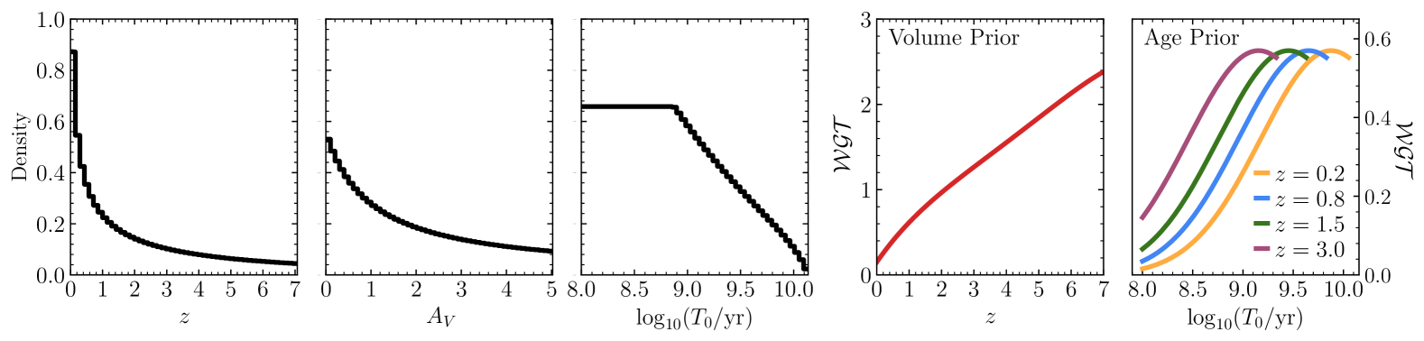
Figure 1: Left panels: distribution of redshifts $z$, attenuations $A_{v}$, and ages $T_{0}$ for the reference sample used in this work. Right panels: the two priors adopted in this work – volume and age – as multiplicative weights on the reference galaxies, depending on their redshifts or ages.

The reference sample differs from the one used to produce the Q1 data products, the reason for which will be clear in a few paragraphs. It has been built from a grid of templates (Bruzual & Charlot 2003, in the 2016 version), using the MILES stellar library, which adopts the Kroupa (2001) IMF, which we therefore converted to Chabrier (2003) for PPs. The models have been built with exponentially delayed star-formation histories:

$$\mathrm{SFR}(t)\propto(t-T_{0})\,\mathrm{e}^{-(t-T_{0}/\tau)},$$ (1)

drawn from a Halton (1964) grid in a 6-dimensional space with the following free parameters:

• redshifts: $0<z<7$;

• ages: $8<\log_{10}(T_{0}/\mathrm{yr})<10.138$;

• e-folding timescale: $8<\log_{10}(\tau/\mathrm{yr})<10.5$;

• ionisation parameter: $-4<\log_{10}(U)<-2$;

• metallicities: $0.1<Z/Z_{\odot}<2$.

For dust attenuation, we generate models with both Calzetti et al. (2000) and SMC (Prevot et al. 1984) laws, with $V$-band attenuation $A_{V}$ between $0$ and $5$. Stellar masses and SFRs are inferred from the amplitude of the observed spectral energy distribution (SED), as a scaling parameter recovered by nnpz. Metallicities and ionisation parameters are distributed uniformly within the given ranges; the same for $\tau$, but on a logarithmic scale. The redshifts are distributed with a linear scaling in $(1+z)$ steps, while ages and $A_{V}$ scale logarithmically from the lowest value to the highest. For these last three parameters, their distribution in the reference sample is shown in black in the first three panels of Fig. 1. We then generate the noise-free observed-frame photometry associated with each model. In the end, the reference sample consists of $1\,490\,150$ objects.

nnpz then finds the $80$ NNs for every target galaxy, based on the observed magnitudes and colours. Each of these NNs will have its own weight – measured from the $\chi^{2}$ distance between the reference and the target – and scaling parameter from the SED amplitude. By combining them, we measure the median (or the mode) of the distribution of NNs, which ultimately are the inferred photo-$z$s, PPs, and absolute magnitudes of the target galaxies.

Differently from what has been done in the Euclid pipeline, we add two more photometric points to the reference sample, accounting for the IRAC1 and IRAC2 channels (see Sect. 2). Moreover, having access to the nnpz results – that is, the set of NNs for each target galaxy – we can impose whatever physically motivated condition (i.e., a prior) directly on the NNs, either by measuring the output $z_{\rm phot}$ or PPs only on the set of NNs that satisfy the condition, or by re-weighting differently the NNs in the reference sample in order to penalise unphysical solutions.

As reported in Sect. 6.1.1 of Euclid Collaboration: Tucci et al. (2025), the Q1 pipeline results (obtained without the application of any condition to the NNs) contain an artificially high number of low-$z$ galaxies with extremely young ages – $\log_{10}(T_{0}/\mathrm{yr})$ starts from $7$ in the pipeline – observed at the peak of their star-forming activity, thus at the limit of specific star-formation rate (sSFR) inherent to parametric models ($\log_{10}\mathrm{sSFR/\mathrm{yr}^{-1}}\simeq-7.8$, see Fig. 8 of Ciesla et al. 2017). The resulting redshift distribution is ultimately skewed towards non-physically high number counts at low-$z$, creating an artefact straight line at the sSFR saturation limit in the SFMS plot (see Fig. 14 in Euclid Collaboration: Tucci et al. 2025). In principle, this issue could be addressed in the Q1 pipeline data product by imposing an age prior on the NNs, for example, ignoring those with ages $<0.1\,\mathrm{Gyr}$. This would significantly reduce the impact of artefacts, but at the cost of reducing the Q1 sample by about $40\%$, excluding from the sample all sources without even a single NN that satisfies the prior. Losing these sources would introduce systematic biases in our analysis. To avoid this, we take some precautions that deviate from what has been done in the pipeline, in order to reduce the impact of those artefact sources without losing a significant fraction of the sample: the boundaries for ages and $A_{\mathrm{V}}$ mentioned above used to generate the reference sample for this work are different from those reported in Euclid Collaboration: Tucci et al. (2025), with $0<A_{\mathrm{V}}<3$ and $7<\log_{10}(T_{0}/\mathrm{yr})<10.138$. We also increase the $k$–number of NNs to $80$. Finally, we impose both a volume and an age prior to the NNs in the reference sample.

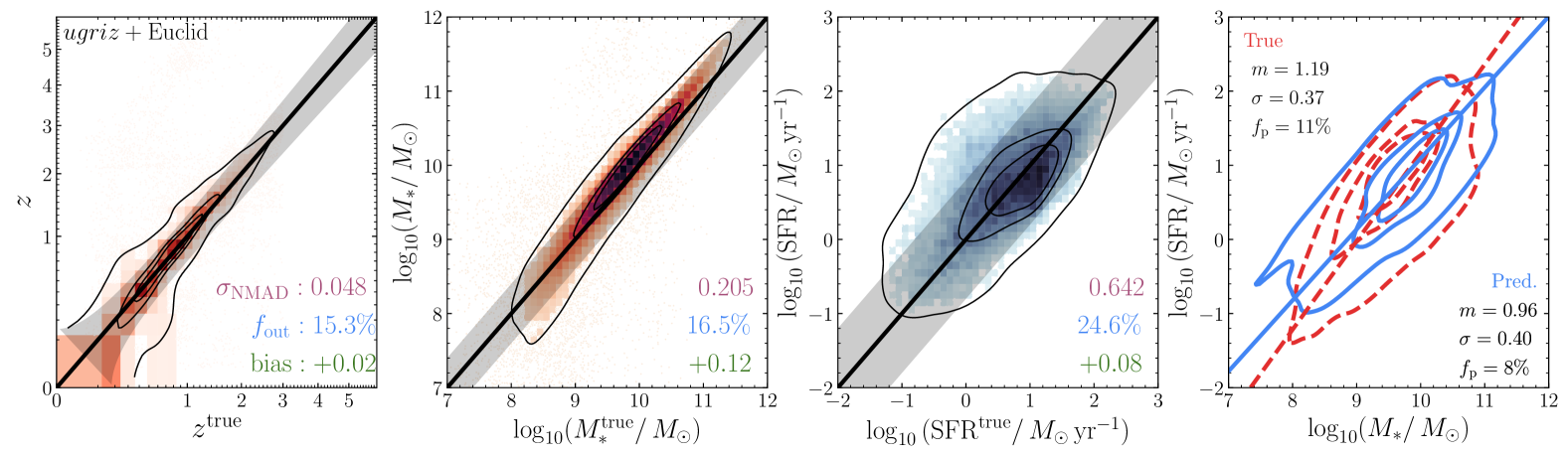
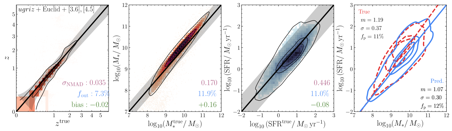
Figure 2: Results for the nnpz run on the FS2 galaxies, without (top panels) and with the first two WISE filters (bottom panels). The black line is the 1:1 relation; the shaded area is the region beyond which a prediction is an outlier. In every plot, the contours are the area containing $86\%$, $39\%$ (corresponding to the $2\sigma$ and $1\sigma$ levels for a 2D histogram) and $20\%$ of the sample. For SFMS (right panel) the true distribution is reported in red (dashed), the predicted one in blue (solid). The lines are the ODR best-fit to the distribution with passive galaxies removed. The reported metrics are NMAD (purple), the outlier fraction $f_{\rm out}$ (blue), and the bias (green) for the photometric redshifts and physical parameters, and the slope $m$, scatter $\sigma$, and fraction of passive galaxies $f_{\rm p}$ for the SFMS, all defined in Sect. 3.1.

With the volume prior, we increase the weights of NNs at higher redshifts compared to those at lower redshifts, where the volume of the Universe sampled by the survey is smaller and fewer galaxies are expected to be observed. This prior is implemented as a multiplicative weight assigned to each object in the reference sample, and only depends on the redshift as

$$\mathcal{WGT}(z)\propto\frac{{\rm d}V_{\rm c}(z)}{{\rm d}z},$$ (2)

where ${\rm d}V_{\rm c}(z)$ is the comoving volume shell in the interval $[z,\,z+\mathrm{d}z]$. This prior is shown in red in the centre-right panel of Fig. 1.

The age prior is once again a multiplicative weight $\mathcal{WGT}(T_{0})$ to apply on NNs. This takes into account the fact that younger galaxies could be observed at higher redshifts, while this possibility should be reduced at low redshifts. In building the prior, we check the distribution of ages in different redshift bins in the $2\,\mathrm{deg}^{2}$ of the Cosmic Evolution Survey (COSMOS, Weaver et al. 2022), finding that these can be modelled as normal distributions with peak age decreasing while moving at higher redshift. This weight is then constructed as a truncated normal distribution centred at two-thirds the age of the Universe at any given $z$, with width $0.7$ in $\log_{10}(T_{0}/\mathrm{yr})$. A weight equal to zero is assigned for those sources with an age greater than the age of the Universe at the given $z$. The shape of the age prior is reported in the rightmost panel of Fig. 1 for four indicative redshift values.

This procedure makes us sensitive to the bulk of the population of SFGs, while reducing our ability to properly identify and describe outliers (e.g., the starburst galaxies, as the presence of a star-forming burst is not directly accounted for in the reference sample). Given the main scopes of this work, this is acceptable, since it has been found that the exponentially delayed $\tau$ model is an accurate description of the star-formation histories of the main population of SFMS galaxies, at least at $z<2$ (see e.g., Speagle et al. 2014; Ciesla et al. 2017). Recently, studies focussing on non-parametric models of star-formation histories have found how these models could better recover the complex events that arise during the evolution of a galaxy (Iyer et al. 2019; Leja et al. 2019; Baes et al. 2020).

In the future, for Data Release 1, models will better account for starburst galaxies, with the possibility of exploring other regions of the parameter space, even accounting for complex star-formation histories (see for example Euclid Collaboration: Corcho-Caballero et al. 2025).

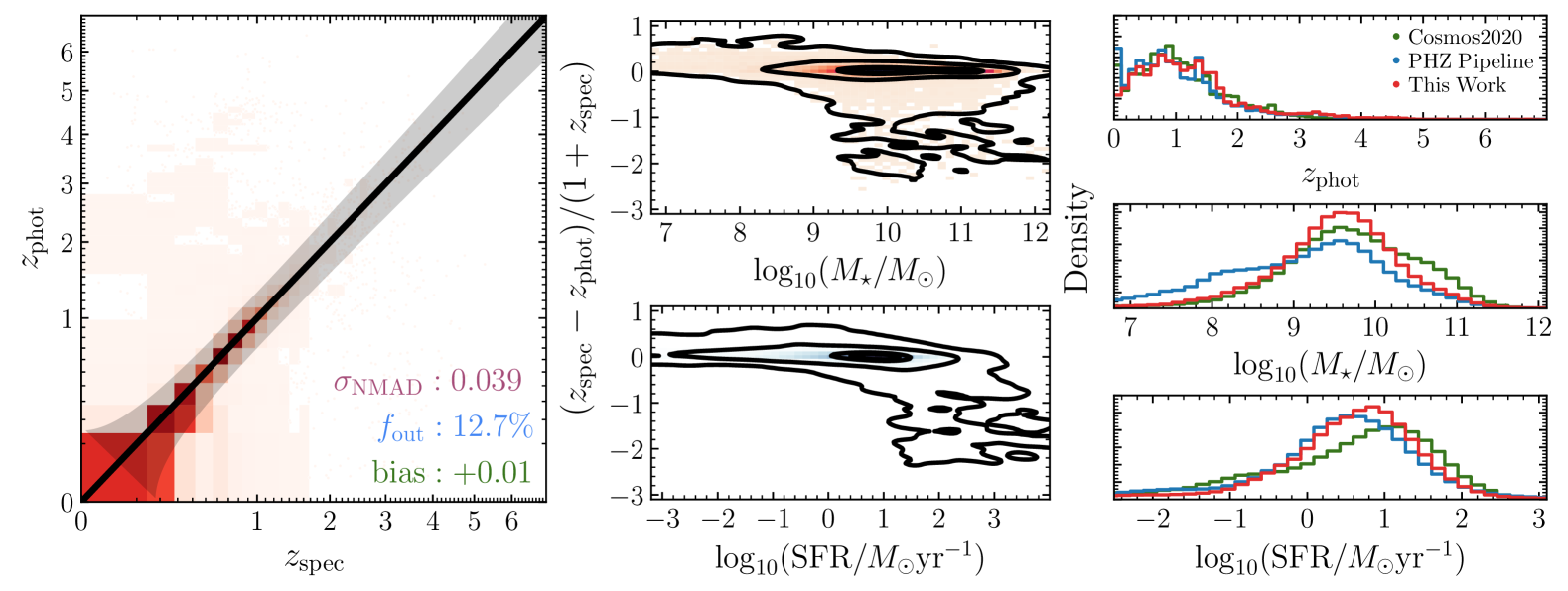
Figure 3: Left: comparison between the measured photometric redshifts and a compilation of all the available and reliable spectroscopic redshifts, colour-coded by the density of objects in each bin. The black line is the 1:1 relation, while the shaded area is the region beyond which a prediction is considered to be an outlier. The reported metrics are NMAD (purple), the outlier fraction $f_{\rm out}$ (blue) and the bias (green), all defined in Sect. 3.1. Middle: normalised redshift difference as a function of stellar masses (top) and SFRs (bottom). The black contours are at the same levels as in Fig. 2. Right: normalised distributions of photometric redshifts (top), stellar masses (centre), and SFRs (bottom) for the our full sample (red), compared with the results coming from the Q1 data products (PHZ, in blue), and COSMOS2020 (green), at the same magnitude cuts applied in this work (see Sect. 2).

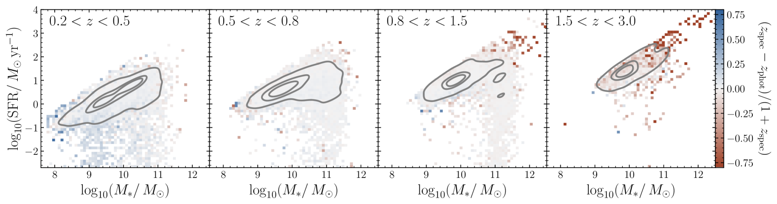
Figure 4: The $M_{\ast}$–SFR plane in four different redshift intervals, only for the sources with a reliable $z_{\rm spec}$ described in Sect. 3.3, colour-coded by the median normalized redshift difference in each bin. To give an idea of the density of objects in each redshift interval, we superimpose the contours in gray, with the same levels as in Fig. 2.

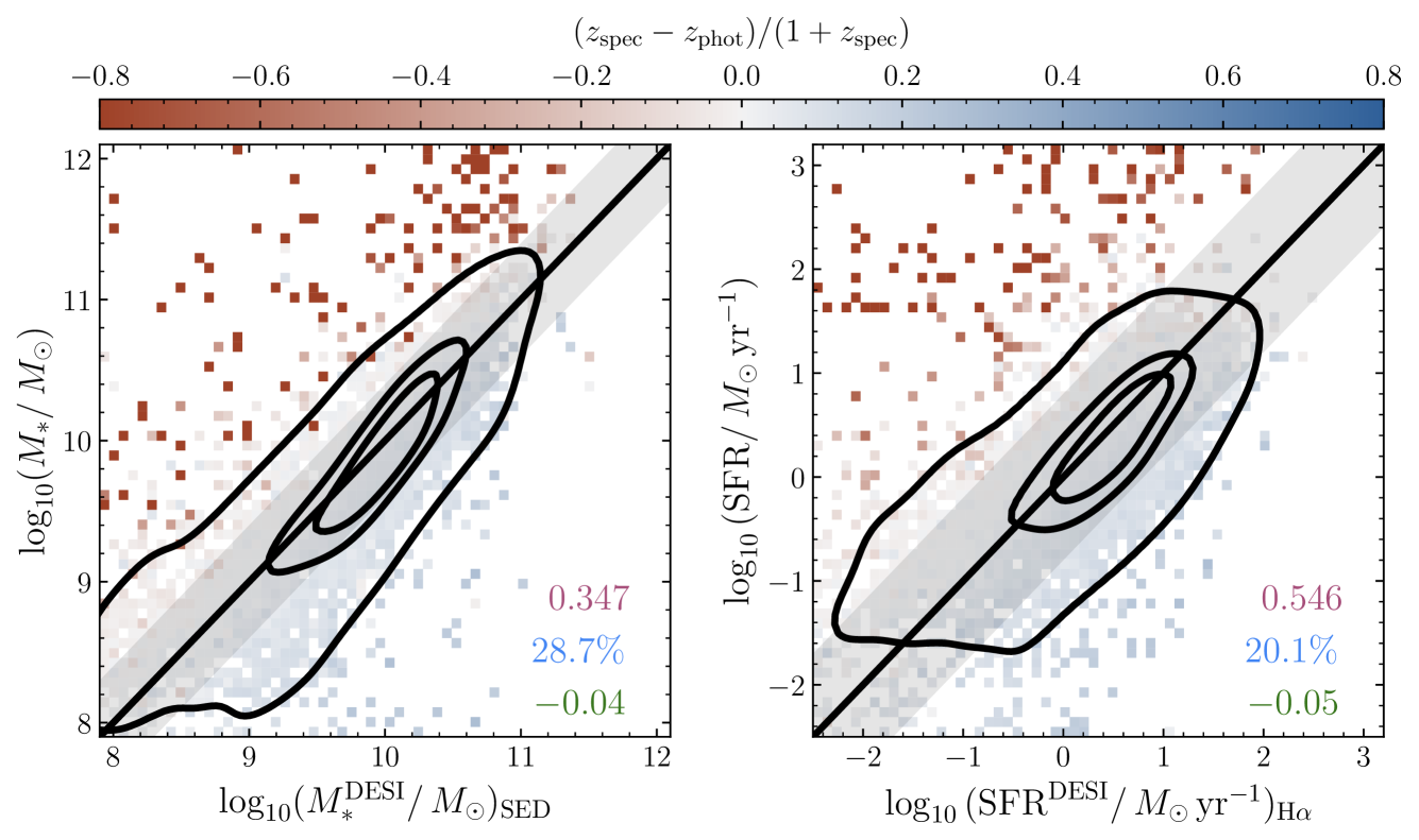
Figure 5: Comparison between the stellar masses and SFRs measured in this work with a sample of objects from DESI with stellar masses from SED fitting (left) and SFRs from H$\alpha$ (right), colour-coded as a function of the median normalised redshift difference in each bin. The black line is the 1:1 relation, while the shaded area is the region beyond which a prediction is an outlier. The contours are the same as in Fig. 2. The reported metrics are defined in Sect. 3.1.

We validate our results both on the available state-of-the-art simulations adapted to reproduce as closely as possible Euclid observations (i.e., the Flagship2 simulation, FS2, see Euclid Collaboration: Castander et al. 2024), and on a compilation of the available spectroscopic redshifts and H$\alpha$ measured SFRs in the EDFs. Although the latter is fundamental to assess the quality of recovered photometric redshifts with what can be interpreted as the closest possible thing to a ground truth value, the former is unavoidable to put a degree of confidence in other recovered quantities such as stellar masses and SFRs.

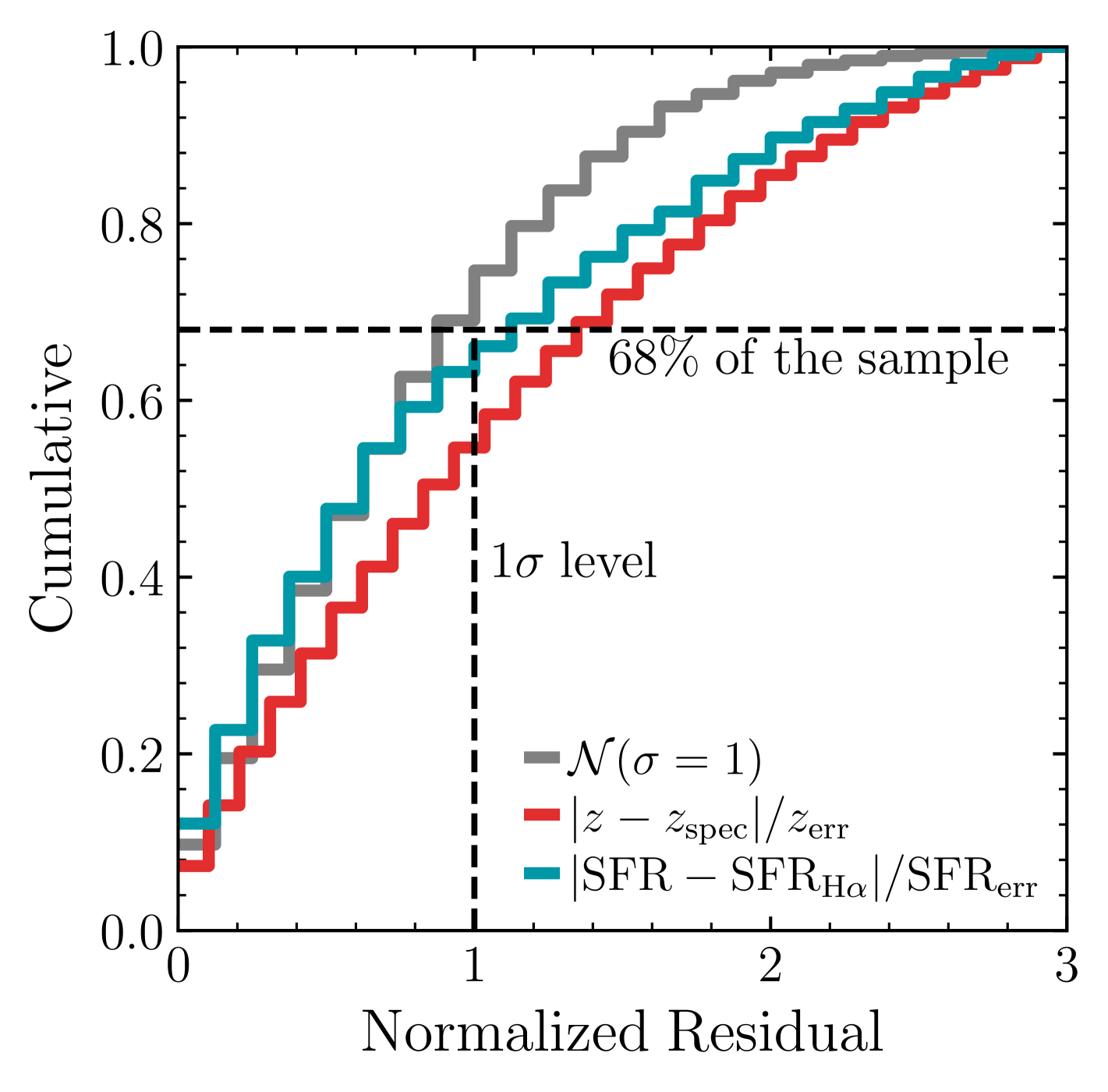
Figure 6: Cumulative distribution of the normalized residuals for photometric redshifts (red) and SFRs (blue). For comparison, we also show in gray the cumulative of a normal distribution with $\sigma=1$. Dashed black lines highlight the position where $68\%$ of the distributions is, and the $1\sigma$ level for the residuals.

3.1 Metrics for quality assessment

The metrics used to quantify the quality of the results are defined differently when referring to redshifts or PPs. We refer the reader to Euclid Collaboration: Enia et al. (2024) for a full discussion of thresholds and catastrophic outlier definitions; here, we simply report the definitions.

We first define a set of true values $z_{\rm test}$ and $y_{\rm test}$ (on a logarithmic scale for PPs), to confront with the predicted values $z_{\rm pred}$ and $y_{\rm pred}$. We then define the normalised median absolute deviation as

$${\rm NMAD}=1.48\,\times\,{\rm median}\begin{cases}\,\dfrac{|z_{\rm pred}-z_{\rm test}|}{1+z_{\rm test}}-b,&\text{for redshifts,}\\ \,|y_{\rm pred}-y_{\rm test}|-b,&\text{for \lx@glossaries@gls@link{main}{pp}{\leavevmode PPs},}\end{cases}$$ (3)

with $b$ being the model bias (see below).

Then the outlier fraction

$$f_{\rm out}\,=\begin{cases}\,\dfrac{|z_{\rm pred}-z_{\rm test}|}{1+z_{\rm test}}>0.15,&\text{for redshifts,}\\ \,|y_{\rm pred}-y_{\rm test}|>t_{\rm out},&\text{for \lx@glossaries@gls@link{main}{pp}{\leavevmode PPs},}\end{cases}$$ (4)

with $t_{\rm out}=0.4$ for stellar masses and $t_{\rm out}=0.8$ for SFRs.

Finally, the bias,

$$b\,={\rm median}\begin{cases}\,\left(\dfrac{z_{\rm pred}-z_{\rm test}}{1+z_{\rm test}}\right),&\text{for redshifts,}\\ \,(y_{\rm pred}-y_{\rm test}),&\text{for \lx@glossaries@gls@link{main}{pp}{\leavevmode PPs}.}\end{cases}$$ (5)

3.2 Validation on simulations

We randomly select about $70\,\mathrm{k}$ sources from a complete octant of the FS2 simulation (Euclid Collaboration: Castander et al. 2024). We checked that the selection does not skew the ground-truth values with respect to the full distribution. These mock sources are, by construction, distributed in the redshift range $0<z<3$, with $6.4<\operatorname{log_{10}}(M_{\ast}/M_{\odot})<12$ and $-4<\operatorname{log_{10}}\,(\mathrm{SFR}/M_{\odot}\,\mathrm{yr}^{-1})<3.1$. We then follow the same procedure described in Sect. 2 of Euclid Collaboration: Enia et al. (2024) to produce a realistic catalogue of mock sources that reproduces as closely as possible what is observed in Q1. We perturb the intrinsic fluxes with the noise level found in Q1 in the same set of filters (see Table 1), and cut at observed magnitudes $H_{\scriptscriptstyle\rm E}<24$. Instead of IRAC, in the FS2 simulation these wavelength ranges are covered by mock observations with WISE bands, W1 and W2 (Wright et al. 2010). Given the similar range covered, we ensure that the resulting performance is comparable if not exactly the same.

We then run nnpz with the same reference sample described in Sect. 3, one run with the WISE filters and one without, and produce the recovered results as the median of the 80 NNs. The results are shown in Fig. 2, where we report the recovered versus true relation without (top panel) and with (bottom panel) the two WISE filters. These results follow closely what has already been described in Euclid Collaboration: Enia et al. (2024), at least at the order of magnitude level. It is immediately noticeable how the addition of the two filters at $3.6\,$\mathrm{\SIUnitSymbolMicro m}$$ and $4.5\,$\mathrm{\SIUnitSymbolMicro m}$$ improves parameter estimation, with photo-$z$ NMADs and the outlier fraction decreasing from $0.048$ to $0.035$ and from $15\%$ to $7\%$, respectively. The same holds for stellar masses (NMAD decreasing from $0.206$ to $0.170$ and the outlier fraction from $17\%$ to $12\%$) and especially for SFRs (NMAD decreasing from $0.643$ to $0.446$ and the outlier fraction from $25\%$ to $11\%$). As expected, the recovery of SFMS improves with respect to the case without the two filters in NIR, with a much better recovery of the slope and normalisation of the SFMS relation.

3.3 Photometric redshifts and PPs validation

Quality assessment for the redshifts is performed by looking at how they compare with respect to observed spectroscopic ones. The EDFs cover regions of the sky where there is a plethora of coverage from other spectroscopic surveys. In total, we successfully match $63\,504$ galaxies with a reliable spectroscopic redshift, that is, with a redshift quality flag of 3 or 4 (see description in Sect. 5.2 of Euclid Collaboration: Tucci et al. 2025). These $z_{\rm spec}$ values are from: the Dark Energy Spectroscopic Instrument (DESI, DESI Collaboration et al. 2016, 2024); the 16th Data Release of the Sloan Digital Sky Survey (SDSS, Ahumada et al. 2020); the 2MASS Redshift Survey (2MRS, Huchra et al. 2012); the PRIsm MUlti-object Survey (PRIMUS, Coil et al. 2011); the Australian Dark Energy Survey (OzDES, Yuan et al. 2015; Childress et al. 2017; Lidman et al. 2020); 3dHST (Brammer et al. 2012); the 2-degree Field Galaxy Redshift Survey (2dFGRS, Colless et al. 2001); the 6-degree Field Galaxy Redshift Survey (6dFGS, Jones et al. 2009); the MOSFIRE Deep Evolution Field Survey (MOSDEF, Kriek et al. 2015); the VANDELS ESO public spectroscopic survey (Pentericci et al. 2018; Talia et al. 2023); the JWST Advanced Deep Extragalactic Survey DR3 (JADES, D’Eugenio et al. 2024); the 2-degree Field Lensing Survey (2dFLens, Blake et al. 2016); and the VIMOS VLT deep survey (VVDS, Le Fèvre et al. 2005).

The results are reported in Fig. 3. In the left panel, we compare the photometric versus spectroscopic redshifts for the subset of reliable spectroscopic redshifts in our sample. These are almost equally divided between EDF-F and EDF-N, with only a handful ($123$) of objects in EDF-S. The trend we find using Euclid real data is similar to what is shown in the previous section, with a non-negligible improvement when adding the two IRAC bands. In particular, compared to the same analysis performed without the addition of the two IRAC bands, the NMAD decreases from $0.06$ to $0.04$ and the fraction of outliers decreases from $26\%$ to $13\%$. In the central panels, we plot the normalised difference between spectroscopic and photometric redshifts, as a function of the stellar masses and the SFRs. We do not observe any troubling systematic trend, with the exception of the (expected) behaviour in which galaxies mistakenly placed at higher redshift – mostly those with $(z_{\rm spec}-z_{\rm phot})/(1+z_{\rm spec})>-1$ – are found with a wrong higher SFRs, so some caution must be taken when dealing with those high-$z$ galaxies, or with $\operatorname{log_{10}}\,(\mathrm{SFR}/M_{\odot}\,\mathrm{yr}^{-1})>2.4$.

When looking at the full sample of objects – not just spectroscopic ones – there are no ground-truth values to compare with, but we can still investigate how our results agree with the full distribution of photometric redshifts, stellar masses, and SFRs, especially when compared with other surveys. This is done in the right panels in Fig. 3, where we compare our results for the full sample (in red) with what is observed in COSMOS (in green), at the same magnitude cut applied in this work (i.e., $H_{\scriptscriptstyle\rm E}<24$), and with the same inferred PPs from the Q1 data products (PHZ, in blue). The first two distributions in redshift are comparable, with the main differences observed in a slightly lower fraction of $0.6<z<1.2$ objects in our sample (and conversely, a few more $z>3$ galaxies), while the Q1 data products exhibit a significantly greater number of $z<0.2$ objects. As for the stellar masses, our results improve with respect to the almost flat at $8<\operatorname{log_{10}}(M_{\ast}/M_{\odot})<9$ distributions of Q1 data products; however, we find relatively fewer objects in the $10.2<\operatorname{log_{10}}(M_{\ast}/M_{\odot})<11.2$ range and conversely more in the $9.2<\operatorname{log_{10}}(M_{\ast}/M_{\odot})<10.2$ range with respect to COSMOS.

In Fig. 4 we report all these information into the $M_{\ast}$–SFR plane, where the SFMS in observed and the main goal of this work. For the subsample of sources with reliable spectroscopic redshift, we plot the median value of the normalized redshift difference in each bin, with red colours highlighting sources mistakenly placed at a higher redshift, and blue colours the opposite. While the latter catastrophic outliers are a small issue only visible in the first redshift interval (with $0.2<z<0.5$), the former becomes more and more prominent at higher redshifts (i.e., $z>1.5$), introducing a non-negligible bias in the estimates of $M_{\ast}$ and SFR in the highest mass and SFR regimes, with these skewed towards higher values due to the wrong redshift attribution.

We compare the measured PPs with the ones in the value-added catalogue of PPs in DESI (Siudek et al. 2024), although for a limited number of sources ($\sim 5\,\mathrm{k}$) in the interval $0<z<0.6$. In particular, we confront the SFRs with those obtained from both H$\alpha$ and H$\beta$ line measurement – not exactly ”ground truth” values, but close – while the stellar masses are compared to their SED fitting results. The IMF is the same as the one adopted for this work (Chabrier 2003), and SFRs are obtained from H$\alpha$ following Kennicutt (1998a). The results are shown in Fig. 5, where the results for each PP is colour-coded as a function of the median value of $(z_{\rm spec}-z_{\rm phot})/(1+z_{\rm spec})$ in each bin. Despite the limited sample, the performance is in line with what is expected from the simulations. It is immediately clear how the vast majority of catastrophic outliers (i.e., where PPs fall outside of the defined thresholds) are a consequence of sources with a wrong photometric redshift estimate.

Finally, we used these SFRs from H$\alpha$ and the reliable spectroscopic redshift sample to place some constraints on the estimated uncertainties in the photo-$z$s and SFRs. Uncertainties are measured from the $16$th and $84$th percentiles of the weighted distribution of NNs (see Sect. 3). To account for the possibility of an under- (or over-) estimation of those uncertainties, we look at the cumulative distribution of $(z_{\rm phot}-z_{\rm spec})/z_{\rm err}$ – and similarly $(\mathrm{SFR}-\mathrm{SFR}_{\rm H\alpha})/\mathrm{SFR}_{\rm err}$ – where we expect $68\%$ of these to fall below $1$ if the uncertainties are well-estimated. In contrast, an underestimate would lead to fewer sources within the $1\sigma$ limit, and the opposite would be true for an overestimate. These cumulative distributions (normalized residuals, red for redshifts and blue for SFRs) are reported in Fig. 6. We find that our uncertainties are slightly underestimated for redshifts ($1\sigma$ level reached for $55\%$ of the sample) and almost spot on for SFRs. We estimate the underestimation of the uncertainties of the photometric redshifts to be a factor of about $1.5$.

We take the mode of the distribution of uncertainties as the typical values for each parameter, which are $0.05$ for redshifts, $0.11$ for stellar masses, and $0.08$ for SFRs (on a logarithmic scale). The typical uncertainty on SFRs will be used in the following section for the fit of the SFMS.

4 Results

We start from the sample described in Sect. 2, and limit our analysis to the redshift range between $0.2$ and $3.0$. This is motivated by the need to obtain a statistically reliable sample in terms of mass completeness and quality of the recovered photometric redshifts and physical properties. In Euclid Collaboration: Enia et al. (2024) it is shown how the main source of biases in the analysis of SFMS during cosmic time – apart from the inherent dispersions in determining the correct PPs– arises from the photo-$z$ estimation, where typically some low-$z$ objects are placed at high-$z$ (up to around $10\%$ of catastrophic outliers) with increased stellar masses and SFRs. The net effect is a steepening of the SFMS at lower redshifts, and the opposite at higher $z$ (see Fig. 11 of Euclid Collaboration: Enia et al. 2024). This is also observed in the validation tests that we performed with simulations and reported in Sect. 3.3 (see Fig. 4).

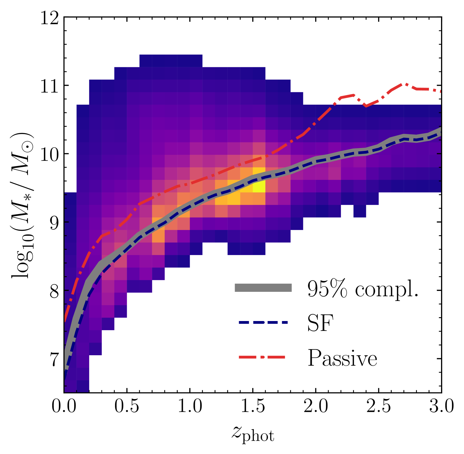
Figure 7: The stellar mass completeness for the sample used in this work (Pozzetti et al. 2010), with a cut at $H_{\scriptscriptstyle\rm E}<24$, shown as the density of galaxies in the photometric redshifts vs. stellar masses plane. Gray solid line is the $95\%$ stellar mass completeness limit, red dashed-dotted line for passive galaxies, and blue dashed line for SFGs.

We perform our subsequent analysis in the following redshift bins: $[0.2$, $0.5],[0.5$, $0.8],[0.8$, $1.5],[1.5$, $3.0]$, with the exception of the morphological analysis, where we stop at $z=1.5$, since for higher redshifts the quality of the recovered morphological parameters is limited by the sizes of the sources reaching the resolution limit of the survey. Based on the results shown in Fig. 4, we can place a certain degree of confidence in the highest-mass end of the first two redshift intervals, while greater caution is required for the last two. In each case, we limit our analysis – and the reported values – to $\operatorname{log_{10}}(M_{\ast}/M_{\odot})<11.5$.

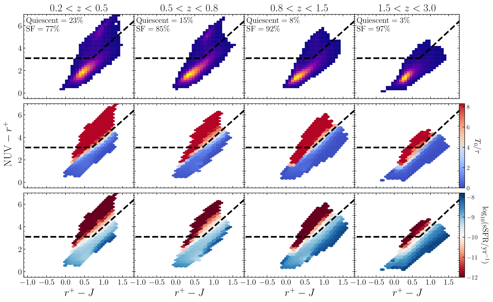
Figure 8: $\mathrm{NUV}-r^{+}$ versus $r^{+}-J$ rest-frame colours for the sources above the $95\%$ mass completeness limit, in four redshift bins, colour-coded with the density of objects (upper panels), the ratio between $T_{0}$ and $\tau$ (middle panels), and the sSFR (bottom panels). Dashed-dotted lines divide the regions between star-forming and quiescent galaxies, following the criteria presented in Ilbert et al. (2013).

4.1 Mass completeness

We estimate the mass completeness of the sample limited to $H_{\scriptscriptstyle\rm E}<24$ following the method described in Pozzetti et al. (2010). We select galaxies close to the limiting magnitude of our sample, that is, those with $23<H_{\scriptscriptstyle\rm E}<24$ (with identical results of choosing the faintest $20\%$ as in Pozzetti et al. 2010), and measure for each galaxy

$$\log_{10}(M_{\rm lim}/M_{\odot})=\operatorname{log_{10}}(M_{\ast}/M_{\odot})-0.4(H_{\scriptscriptstyle\rm E}-24),$$ (6)

representing the mass the galaxies would have at the limiting magnitude. We then measure the $95$ percentile of the distribution of $M_{\rm lim}(z)$ for each redshift bin. This is reported in Fig. 7. The classification into star-forming (blue dashed line) and passive galaxies (red dashed-dotted line) is done with the selection criteria based on the $\mathrm{NUV}$–$r^{+}$–$J$ diagram (as explained below).

The sample is around $95\%$ complete for $M_{\ast}$ that increases from $\operatorname{log_{10}}(M_{\ast}/M_{\odot})\sim 7$ (at $z\sim 0.1$) to $\sim 9$ (at $z\sim 1$), and increases from $\operatorname{log_{10}}(M_{\ast}/M_{\odot})\sim 9.5$ to $\operatorname{log_{10}}(M_{\ast}/M_{\odot})\sim 10$ while going to higher redshifts, from $z=1.5$ to $2.5$. For passive galaxies, the limit is $0.3$ – $0.4\,\mathrm{dex}$ higher up to $z\sim 1.8$, and about $0.7\,\mathrm{dex}$ higher at $z>2$.

4.2 Star-forming and passive galaxy classification

Colour-based classifications of galaxies use the principle of separating red and blue galaxies and distinguish between dusty and intrinsically red ones (e.g., the $U-V$ versus $V-J$ colour diagram Labbé et al. 2005; Wuyts et al. 2007; Williams et al. 2010). In this work we use the $\mathrm{NUV}-r^{+}$, $r^{+}-J$ colours (Ilbert et al. 2010), where star-forming and passive galaxies are discriminated based on their absolute $\mathrm{NUV}$, $r^{+}$, and $J$ magnitudes, with quiescent galaxies satisfying the following relations:

$$\mathrm{NUV}-r^{+} > 3(r^{+}-J)+1;$$

$$\mathrm{NUV}-r^{+} > 3.1.$$ (7)

This combination of criteria works in a similar fashion to the $UVJ$ diagram but is more sensitive to recent star-formation via the $\mathrm{NUV}-r^{+}$ colour, which separates passive (redder) and star-forming (bluer) galaxies (Ilbert et al. 2013; Arnouts et al. 2013). Truly passive galaxies are then distinguished from dusty, star-forming objects via the $r^{+}-J$ colour, ensuring a proper separation between the two different populations.

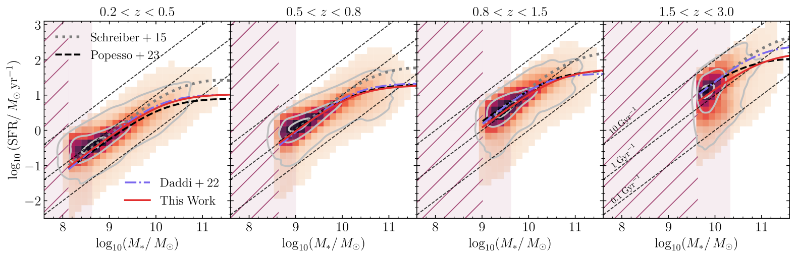
Figure 9: The $\mathrm{SFR}$–$M_{\ast}$ relation for SFGs, selected with the $\mathrm{NUV}-r^{+}$ versus $r^{+}-J$ condition, coloured by the density of objects in each redshift bin. Within the coloured bins there is $99.9\%$ of the sample of SFGs, while the gray contours are the lines enclosing $95\%$, $50\%$, and $10\%$ of it. The red line is the fitted SFMS presented in this work, starting from the completeness limit mass at the start of the $z$-bin. The other SFMS s are from Popesso et al. (2023, dashed black line), Schreiber et al. (2015, dotted gray line), and Daddi et al. (2022a, dashed-dotted blue line), all evaluated at the median redshift of each redshift bin (or to the closest reported value). The purple shaded regions highlights where the mass is below the completeness limit at the start (hatched) and at the end of the redshift bin. Dashed gray lines highlight the region of constant sSFR.

The colours $\mathrm{NUV}-r^{+}$ versus $r^{+}-J$ of our sample are shown in Fig. 8, colour-coded as a function of the number density of objects with certain colours (top panels) and the median $T_{0}/\tau$ (middle panels) and sSFR in each bin (bottom panels), in the four different redshift bins. Only objects whose mass is higher than the $M_{\lim}(z)$ value at the $z_{\rm min}$ of the redshift bin are shown, to account for sample incompleteness (see Fig. 7). To be consistent with the selection criteria reported above, the adopted absolute magnitude $J$ is not the one estimated in the rest frame Euclid $J_{\scriptscriptstyle\rm E}$ filter but in the $J_{\scriptscriptstyle\rm UltraVISTA}$ filter (Euclid Collaboration: Schirmer et al. 2022); similarly, we adopt the $r^{+}$ band as in Ilbert et al. (2010).

We recover the well-known increase in the fraction of passive galaxies while going to later times, highlighting the assembly of the population of quiescent galaxies observed in the Universe. When checking the colour diagrams against the measured values of sSFR, we notice the presence of a small fraction of objects ($\sim 3\%$) outside the boundaries for quiescent galaxies in the $\mathrm{NUV}$–$r^{+}$–$J$ diagram, but with a median value of $\log_{10}(\mathrm{sSFR}/\mathrm{yr}^{-1})<-11$ (and $T_{0}/\tau>8$), that is, in a region of the $M_{\ast}$–SFR plane where we would expect only quiescent galaxies. This is a small, negligible number of interlopers, reassuring about the goodness of the classification based on the rest-frame colours.

4.3 The SFR–$M_{\ast}$ relation in the EDFs

The $M_{\ast}$–SFR plane for the sample of SFGs selected with the $\mathrm{NUV}$–$r^{+}$–$J$ colours is shown in Fig. 9, in four redshift bins, colour-coded in terms of the logarithmic density of objects per bin. The SFMS is observed up to the highest redshift bin ($z<3$). In the plot, we report three previously published SFMS relations for comparison: Eq. (15) of Popesso et al. (2023, black dashed line), that is, a comprehensive compilation of 27 literature SFMS relations fitted to the same functional form, in the mass range $8.5<\operatorname{log_{10}}(M_{\ast}/M_{\odot})<11.5$; Schreiber et al. (2015, gray dotted line), obtained from $\sim 10\,\mathrm{k}$ galaxies with the deepest Herschel observations of the GOODS and CANDELS-Herschel programme, with $9.5<\operatorname{log_{10}}(M_{\ast}/M_{\odot})<11.5$; Daddi et al. (2022a, blue dashed-dotted line), obtained from a stacking analysis of $\sim 400\,\mathrm{k}$ colour-selected SFGs in COSMOS (Delvecchio et al. 2021), here too in the mass range $8.5<\operatorname{log_{10}}(M_{\ast}/M_{\odot})<11.5)$.

All these SFMS forms include the presence of a bending of the relation at the high-mass end. Having enough statistics in terms of the number of objects per bin, we can significantly constrain the deviation from the linear form at high masses. For example, in each redshift interval Delvecchio et al. (2021), Daddi et al. (2022a) found no more than $838$ SFGs at $\operatorname{log_{10}}(M_{\ast}/M_{\odot})>11$, and in the same mass range the stacking analysis in Schreiber et al. (2015) has $<15$ galaxies per bin. Analogously, most of the studies in the compilation of Popesso et al. (2023) stop at $\operatorname{log_{10}}(M_{\ast}/M_{\odot})=11$, and those who extend further never reach more than $10^{3}$ galaxies per bin in comparable redshift ranges. Due to the large area observed in Q1, the minimum number of galaxies we have at $\operatorname{log_{10}}(M_{\ast}/M_{\odot})>11$ is $875$, in the $[0.2$, $0.5]$ redshift bin. This number increases to $7640$ (for $0.5<z<0.8$), $18951$ (for $0.8<z<1.5$), and $8165$ (for $1.5<z<3.0$), one or two orders of magnitude higher than the former reported statistics. These numbers are more than enough to subdivide the $\operatorname{log_{10}}(M_{\ast}/M_{\odot})>11$ region into two different bins at $z>0.8$, to better constrain the part of the SFMS where the SFR appears to saturate. The same reasoning, scaled by an order of magnitude, applies if we consider $\operatorname{log_{10}}(M_{\ast}/M_{\odot})>10.5$.

Our fit to the observed data is the red line in Fig. 9. Overall, the fits in Popesso et al. (2023) and Daddi et al. (2022a) more resemble our results, while Schreiber et al. (2015) find systematically higher SFRs at the highest mass end. The functional form that we fit these data to, first proposed by Lee et al. (2015), is the same as in Eq. (15) of Popesso et al. (2023) or Eq. (1) of Daddi et al. (2022a)

$$\mathrm{SFR}=\frac{\mathrm{SFR}_{\rm max}}{1+(M_{0}/M_{\ast})^{\gamma}},$$ (8)

that is, a parameterisation where the SFR is linked to the stellar mass through three parameters: the bending mass after which the relation deviates from the linear behaviour ($M_{0}$); the maximum SFR for $M_{\ast}\gg M_{0}$ ($\mathrm{SFR}_{\mathrm{max}}$); and the slope of the linear relation when $M_{\ast}\ll M_{0}$ ($\gamma$). These parameters have been shown to be directly linked to fundamental properties in models of gas accretion (e.g., the bending mass $M_{0}$ is directly linked to the ratio between $M_{\rm shock}$ and $M_{\rm stream}$, see Daddi et al. 2022a, b). For each fit, we keep $\gamma$ fixed at $1.0$, as it has been shown to be a representative value around which almost every fit converges at different redshifts (see Lee et al. 2015; Popesso et al. 2023; Daddi et al. 2022a). This also makes possible a direct comparison with these works in terms of bending mass and maximum SFR.

When fitting the SFMS, we must take into account the fact that for each redshift bin, there are two possible values for the mass completeness limit, depending on whether consider the mass at the lower limit of the redshift bin $z_{\rm start}$ or at the higher limit $z_{\rm end}$. Depending on the width of the redshift bin, these two masses can differ significantly, of the order of $0.4$ – $0.6\,\mathrm{dex}$ (see Fig. 9). When $M_{\ast}>M_{\rm lim}(z_{\rm end})$ we are dealing with a complete sample; in this case, we fit the points measured as the median stellar masses and SFRs of the distribution of SFGs in each bin of mass, with associated uncertainty as the quadrature sum of the standard deviation of the median in each bin and the typical uncertainty on the SFRs (see Sect. 3.3). These are shown as stars in the bottom panel of Fig. 10, coloured as a function of the redshift bin to which they belong. When $M_{\ast}<M_{\rm lim}(z_{\rm start})$ we consider the sample to be incomplete, and these galaxies are excluded from the fit. In the mass bins where $M_{\rm lim}(z_{\rm start})<M_{\ast}<M_{\rm lim}(z_{\rm end})$, we are preferentially missing lower-mass galaxies, which tend to have lower SFR. As a result, we treat the SFR data points in these bins as upper limits, as indicated by the arrows in the bottom panel of Fig. 10.

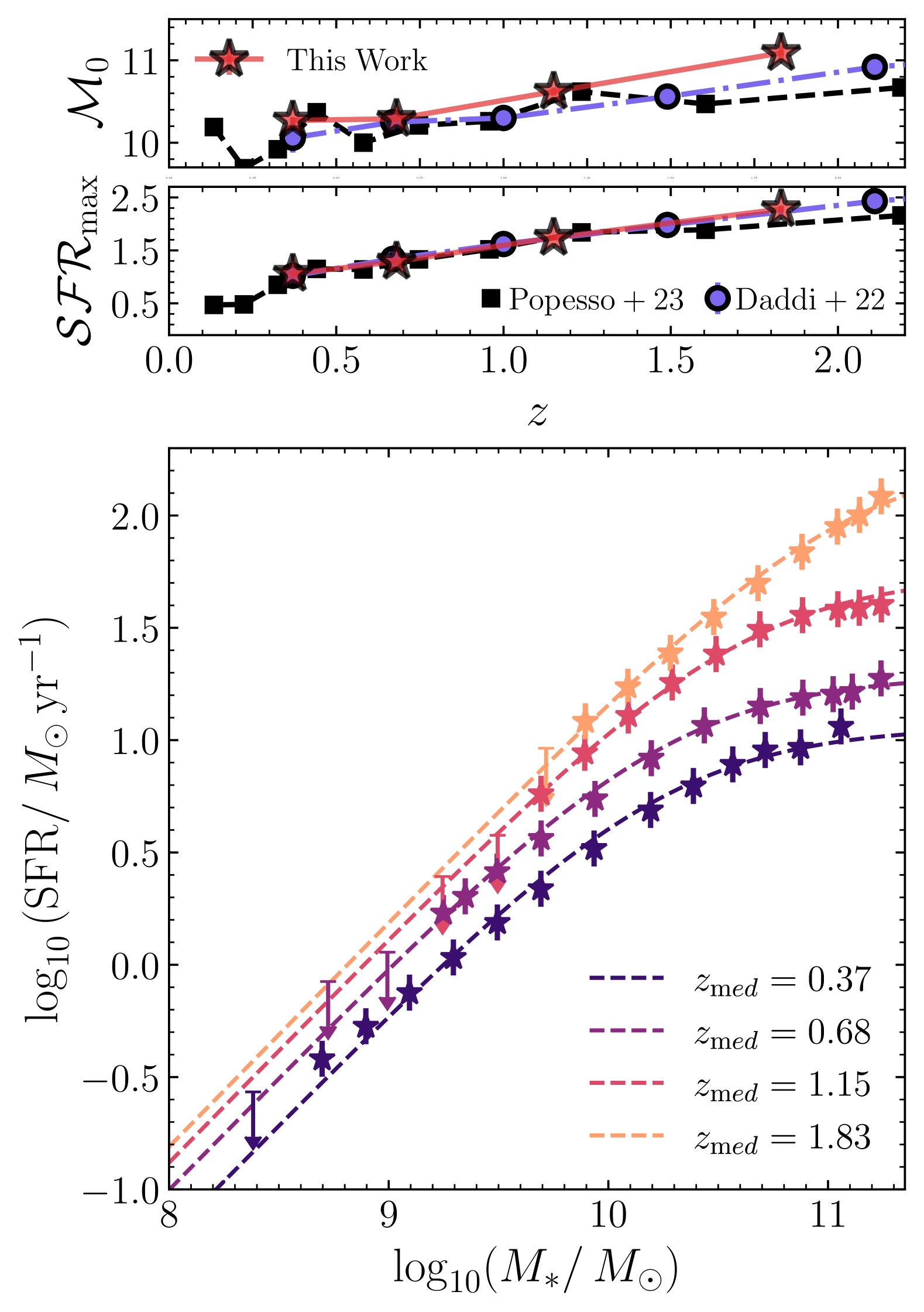
Figure 10: Lower panel: our fit of the SFMS, in the four redshift bins (stars with error bars and arrows) and best-fit model (dashed lines). The reported redshift is the median $z$ of the bin. Upper panels: the best-fit (red stars) and reported (Popesso et al. 2023, squares for; Daddi et al. 2022a, circles for) values for the bending mass and maximum SFR, defined as $\mathcal{M}_{0}\equiv\log_{10}(M_{0}/M_{\odot})$ and $\mathcal{SFR}_{\rm max}\equiv\log_{10}(\mathrm{SFR}_{\rm max}/M_{\odot}\,\mathrm{yr}^{-1})$, as a function of redshift.

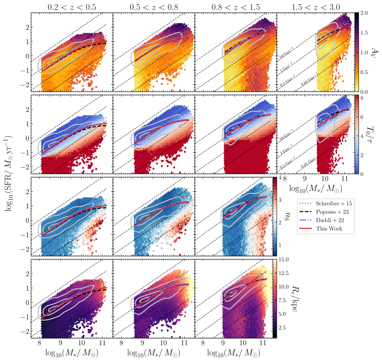
Figure 11: The $\mathrm{SFR}$–$M_{\ast}$ relation, colour-coded by the median $A_{V}$ (top), $T_{0}/\tau$ (middle-top), Srsic index (middle-bottom), and Srsic radius (bottom) of objects in each bin. A bin is coloured only when the number of sources falling within the bin is higher than $20$. The contours in gray contain $90\%$, $50\%$, and $10\%$ of the full sample. The literature SFMS are the same as shown in Fig. 9 and reported in Sect. 4. Dashed lines highlight the loci of equal sSFR.

The SFR–mass bins are obtained by binning the distribution of stellar mass to uniformly cover the stellar masses space with a similar number of sources to make these statistically significant. The bins start from where the stellar mass is higher than the $95\%$ completeness limit at the lower limit of the redshift bin, that is, $\operatorname{log_{10}}(M_{\ast}/M_{\odot})\sim 8.1$ at $z=0.37$, $\operatorname{log_{10}}(M_{\ast}/M_{\odot})\sim 8.6$ at $z=0.67$, $\operatorname{log_{10}}(M_{\ast}/M_{\odot})\sim 9.0$ at $z=1.15$ and $\operatorname{log_{10}}(M_{\ast}/M_{\odot})\sim 9.5$ at $z=1.83$. The results of the fit are reported in Table 2, and showed in Fig. 10 as dashed lines colour coded by redshift bin. The bending mass and maximum SFR are reported as a function of redshift in the upper panels of Fig. 10, as red stars and solid line. We also show, for comparison, the same parameters found in Daddi et al. (2022a, as blue circles and dashed dotted line) and Popesso et al. (2023, black edged squares and dashed line) as a function of $z$.

All bending masses fitted $M_{0}$ increase with redshift. We find results similar to those of Daddi et al. (2022a), with the main difference in the $[0.8$, $1.5]$ bin, with a higher $\log_{10}(M_{0}/M_{\odot})=10.62\pm 0.05$ (similar to what was found in Popesso et al. 2023). In the $[1.5$, $3.0]$ bin, our bending mass is more in line with Daddi et al. (2022a) at $\log_{10}(M_{0}/M_{\odot})=11.10\pm 0.09$, ($0.6\,\mathrm{dex}$ higher than the one in Popesso et al. 2023). However, for this redshift bin, we must again warn the reader about the caveats highlighted in Sect. 3.3 and Fig. 4, that is, at $11<\operatorname{log_{10}}(M_{\ast}/M_{\odot})<11.5$ any wrong redshift attribution will introduce an important source of systematic biases, skewing the fitted bins at higher values of $M_{\ast}$ and SFR, and therefore the recovered $M_{0}$ and $\mathrm{SFR}_{\rm max}$. In any case, the observed agreement and evolution with redshift is remarkable, when taking into account the fact that our SFRs have been evaluated with photometry ranging from the $g$ band (the $u$ band is available only in one field) up to $4.5\,$\mathrm{\SIUnitSymbolMicro m}$$, thus without properly accounting for dust-obscured star-formation processes, which are disentangled from quiescence only when far-IR and submillimetre photometry is available.

Trying to find the best-fit parameters of the SFMS with the functional form in Eq. (8), we also measure the scatter in the relation $\sigma_{\rm SFMS}$, fitting the difference between the observed set of galaxy stellar masses and SFRs and the model as a normal distribution $\mathcal{N}(\sigma_{\rm SFMS})$. We find the same tight scatter $\sigma_{\rm SFMS}\simeq 0.3$ observed in previous studies, consistent in all redshift intervals within the uncertainties (Table 2).

As an internal check, we also fit the same points with a linear relation (e.g., Eq. 10 in Popesso et al. 2023), obtaining worse $\chi^{2}$ for each redshift bin with respect to the relation including the bending at the high-mass end.

Table 2: Fitted values for $\log_{10}(M_{0}/M_{\odot})$, $\log_{10}(\mathrm{SFR}_{\mathrm{max}}/M_{\odot}\,\mathrm{yr}^{-1})$, and the relation scatter $\sigma_{\rm SFMS}$ for each redshift bin, with the median redshift in bin reported in the first column.

$z_{\rm med}$	$\log_{10}(M_{0}/M_{\odot})$	$\log_{10}(\mathrm{SFR}_{\mathrm{max}}/M_{\odot}\,\mathrm{yr}^{-1})$	$\sigma_{\rm SFMS}$
$0.37$	$10.27\pm 0.04$	$1.06\pm 0.03$	$0.34\pm 0.11$
$0.68$	$10.29\pm 0.05$	$1.29\pm 0.03$	$0.27\pm 0.09$
$1.15$	$10.62\pm 0.05$	$1.74\pm 0.04$	$0.28\pm 0.08$
$1.83$	$11.10\pm 0.09$	$2.28\pm 0.07$	$0.40\pm 0.12$

The SFMS dependence on the absorption $A_{V}$ and the ratio between the age and the e-folding time $\tau$ is shown in the first two rows of Fig. 11, where the colours correspond to the median of $A_{V}$ and $T_{0}/\tau$ values of the sources within each bin, with the SFMS contours superimposed in gray. In this case, we do not limit the sample to SFGs only (i.e., we do not remove the sources identified as quiescent in the $\mathrm{NUV}$–$r^{+}$–$J$ diagram), highlighting a bin when the number of sources within the bin is greater than $20$. In this way, we can explore less populated regions of the $M_{\ast}$–SFR plane, where passive galaxies are expected to appear. Of course, the placing in the plane of all the galaxies below a certain limiting sSFR (e.g., $0.01\,\mathrm{Gyr}^{-1}$) should not be considered as absolute, but rather as indicative that those objects are passive galaxies and could lie anywhere below that line. As expected, maximum extinction values ($A_{V}>2.0$) are associated with the most massive and star-forming galaxies of the SFMS, with $1<\mathrm{sSFR}/\mathrm{Gyr}^{-1}<10$, while low or zero dust extinction values are observed at lower sSFRs. Looking at the distribution of fitted $A_{V}$, we recover only a small fraction of objects ($\sim 1\%$) with high extinction $A_{V}>2.5$, with the $A_{V}$ distribution peaking at $0.5<A_{V}<1.0$. This could be due to the particular limitations and caveats of the recovered sample (see Sect. 3), especially in the covered range of wavelengths. Lower sSFR galaxies are associated with stellar populations with older ages, in particular at low redshift, and high age$/\tau$ ratios, while younger ages are found in the upper part of the SFMS and at high redshift (Nersesian et al. 2025).

The morphological parameters for all the Euclid detected sources have been measured by running the SourceXtractor++ code (Bertin et al. 2020; Kümmel et al. 2022), fitting the detections as two-dimensional Srsic profiles (Euclid Collaboration: Romelli et al. 2025, see and Euclid Collaboration: Quilley et al. 2025, for further details). Here, we focus on the Srsic radius $R_{e}$ and the Srsic index $n_{\rm S}$. In order to be more conservative, following what was found in Euclid Collaboration: Quilley et al. (2025, see their Fig. 2), in addition to the cuts described in Sect. 2, we also remove the sources whose fit does not converge to a solution. In these cases the Srsic axis ratio is exactly equal to one, and the Srsic index $n_{\rm S}<0.302$ or $n_{\rm S}>5.45$. These cuts reduce our sample for morphological analysis by $17\%$ leaving a total of $6\,702\,811$ sources.

In the two bottom rows of Fig. 11 we report the SFMS, colour-coded for the median values of $n_{\rm S}$ (middle-bottom row) and $R_{\rm e}$ (bottom row), converted from arcseconds to kiloparsecs for the predicted photo-$z$). We note that the higher values of $n_{\rm S}>3$ are associated with the most massive, low-sSFR objects, and the radii $R_{\rm e}$ increase with stellar mass at all redshifts. In all redshift intervals, the concurrent presence of the SFMS and the prominence of exponential disks with $n_{\rm S}\simeq 1$ (in blue) is immediately visible, while at lower sSFR, close to the limit where measuring SFRs becomes difficult, we note a crowding of sources with de Vaucoulers profiles $n_{\rm S}\simeq 4$ (in red). Between those, an intermediate region of profiles with $2<n_{\rm S}<3$ (the white strip) at about $\mathrm{sSFR}\sim 0.05\,\mathrm{Gyr}^{-1}$, which indicates an evolutionary trend in the structural parameters while moving in the stellar mass–SFR plane, and in total agreement with what has been previously observed in other samples (Wuyts et al. 2011; Martorano et al. 2025). This kind of transition is observed only at the medium-to-high-mass end $\operatorname{log_{10}}(M_{\ast}/M_{\odot})>10$, and appears to show only a weak redshift dependence. Interestingly, the mass over which the sequence of passive $n_{\rm S}\simeq 4$ profiles is observed is almost coincident with the fitted bending mass $M_{0}$.

Euclid combines a large sample area with a uniform multiwavelength view, which has great potential for environmental studies. Despite that, here we do not focus on how the environment shapes the SFMS. These effects are difficult to investigate with Q1 data alone, and for some regimes and for a specific population are studied in other Q1 works (Euclid Collaboration: Cleland et al. 2025; Euclid Collaboration: Mai et al. 2025). The soon-to-be-available DR1 observations of the EDFs are expected to have at least ten ROSs, which corresponds to $1.25$ magnitude-deeper data. Combining the DR1 data, along with other multi-wavelength observations and the Euclid spectroscopy sample, will allow for a thorough investigation of the environmental effects on the SFMS.

5 Conclusions

The Euclid Q1 data release, with its first look at the EDFs, is already a good test of the capabilities of the mission to investigate the formation and evolution of galaxies, especially in terms of the enhanced statistics of such a large area of the extragalactic sky. In this work, we have investigated the relation between stellar masses and SFRs, the SFMS, and how it relates to the other well-constrained PPs and morphological parameters, comparing the results with the existing literature, as a fair validation of the Euclid results and a first exploration of the mission capabilities to return a statistically robust sample. Even a single ROS of the EDFs is able to yield reliable measurements for the photometric redshifts, stellar masses, and SFRs– which in this work have been improved due to the addition of the first two channels of IRAC – for more than eight million galaxies at a magnitude cut of $H_{\scriptscriptstyle\rm E}<24$. In particular, more than $\sim 30\,\mathrm{k}$ galaxies are found with $\operatorname{log_{10}}(M_{\ast}/M_{\odot})>11$, a substantial improvement over all the other extragalactic surveys limited to a few square degrees of the sky.

The recovered scaling relation between stellar mass and SFR is consistent with what is known from previous studies on the SFMS. The data show a similar tight dispersion (between $0.26$ and $0.40\,\mathrm{dex}$), and are in excellent agreement with the functional forms reported in Popesso et al. (2023), Daddi et al. (2022a), and Schreiber et al. (2015). These works fit SFMS with a non-linear term that translates into a bending of the relation, becoming more pronounced at high masses. We fit the relation with the same parameterisation – that is, linking the SFR directly to the bending mass, $M_{0}$, and the star-formation rate maximum, $\mathrm{SFR}_{\mathrm{max}}$ – recovering the same statistical agreement with the previous studies. $M_{0}$ increases almost monotonically with redshift, starting from $\log_{10}(M_{0}/M_{\ast})\simeq 10.3$ at $z=0.37$, up to $11.1$ at Cosmic Noon. Our results are in accord with the presence of this reduction in SFR in massive galaxies, with a better $\chi^{2}$ with respect to a linear one. At the same time, when correlating our results with the catalogue of morphological properties, we recover the well-known bimodality between exponential and smaller star-forming disks and de Vaucoulers profiles for passive and bigger galaxies.