Euclid Quick Data Release (Q1)

Investigating the drivers of the quenching of star formation in galaxies is key to understanding their evolution. The Euclid mission will provide rich spatial and spectral data from optical to infrared wavelengths for millions of galaxies, enabling precise measurements of their star formation histories. Using the first Euclid Quick Data Release (Q1), we developed a probabilistic classification framework, that combines the average specific star-formation rate (${\rm sSFR}_{\tau}$) inferred over two timescales ($\tau={10^{8},10^{9}}$ yr), to categorise galaxies as ‘Ageing’ (secularly evolving), ‘Quenched’ (recently halted star formation), or ‘Retired’ (dominated by old stars). We validated this methodology using synthetic observations from the IllustrisTNG simulation. Two classification methods were employed: a probabilistic approach, integrating posterior distributions, and a model-driven method optimising sample purity and completeness using IllustrisTNG. At $z<0.1$ and $M_{\ast}\gtrsim 3\times 10^{8}\,{M_{\odot}}$, we obtain Euclid class fractions of 68–72%, 8–17%, and 14–19% for Ageing, Quenched, and Retired populations, respectively, consistent with previous studies. Ageing and Retired galaxies dominate at the low- and high-mass end, respectively, while Quenched galaxies surpass the Retired fraction for $M_{\ast}\lesssim 10^{10}\,{M_{\odot}}$.The evolution with redshift shows increasing/decreasing fraction of Ageing/Retired galaxies. The fraction of quenched systems shows a weaker dependence on stellar mass and redshift, varying between 5 and 15$\%$. We find tentative evidence of more massive galaxies usually undergoing quenching episodes at earlier times with respect to their low-mass counterparts. We analysed the mass-size-metallicity relation for each population. Ageing galaxies generally exhibit disc morphologies and low metallicities. Retired galaxies show compact structures and enhanced chemical enrichment, while Quenched galaxies form an intermediate population, more compact and chemically evolved than Ageing systems. Despite potential selection biases, this work demonstrates Euclid’s great potential for elucidating the physical nature of the quenching mechanisms that govern galaxy evolution.

1 Introduction

One of the current central questions in galaxy evolution is understanding the processes that regulate star formation in galaxies. In particular, there are some phenomena, generally known as galaxy quenching, that transform star-forming galaxies, typically characterised by blue colours and high specific star-formation rates (${\rm sSFR}\equiv{\rm SFR}/M_{\ast}$), into quiescent systems dominated by older stellar populations and low star-formation activity. This transition plays a pivotal role in shaping the observed diversity of galaxy populations across time, and is tightly linked to their mass assembly and the large-scale environment they inhabit.

The physical mechanisms driving quenching remain a topic of active research and debate. Two broad categories of processes have been proposed: internally-triggered mechanisms, such as negative feedback from active galactic nuclei (AGN), supernovae-driven winds (Crenshaw et al. 2003; Di Matteo et al. 2005; Croton et al. 2006; Sawala et al. 2010; Cheung et al. 2016; Fitts et al. 2017), which can expel or heat gas, or morpho-kinematic related effects that prevent gas cloud fragmentation (e.g., Bigiel et al. 2008; Martig et al. 2009; Gensior et al. 2020), versus environmentally-driven processes such as ram-pressure stripping (able to remove part of or even all the gas reservoir, e.g. Gunn & Gott 1972; Boselli & Gavazzi 2006; Brown et al. 2017), starvation (the suppression of gas infall; see e.g. Larson et al. 1980; Wetzel et al. 2013; Peng et al. 2015), that leads to a suppression of star formation, or galaxy interactions (Moore et al. 1996; Bialas et al. 2015). These mechanisms often act simultaneously or sequentially, and their relative importance may depend on galaxy mass, environment, and redshift. For example, both theoretical predictions and observational evidence suggest that low-mass galaxies are more strongly affected by environmental effects, whereas massive systems are likely dominated by internal processes like AGN feedback (Peng et al. 2010; De Lucia et al. 2012; Corcho-Caballero et al. 2023a).

The term ‘quenching’ is loosely defined in the literature, encompassing various scenarios (e.g., Faber et al. 2007; Peng et al. 2010; Schawinski et al. 2014). In this work, we define quenching as a process capable of terminating – or significantly suppressing – the star formation of a galaxy on a short timescale relative to the age of the Universe (i.e.lesss than about 1 Gyr). In contrast, we use the term ‘ageing’ to denote the continuous evolution of a galaxy, encompassing different evolutionary stages from star-forming (including short-lived star-burst episodes) to quiescent phases, driven by the steady consumption of its gas reservoir through uninterrupted star-formation (e.g., Casado et al. 2015; Tacchella et al. 2016). Under the ageing scenario, all galaxies eventually become dominated by old stellar populations, turning red naturally. Discriminating between ageing galaxies and systems undergoing ‘slow quenching’ (with timescales $\gtrsim 1$ Gyr, e.g. Schawinski et al. 2014; Moutard et al. 2016; Belli et al. 2019; Tacchella et al. 2022) is challenging and, in practice, often impossible. Therefore, we focus on galaxies with evidence of recent ‘fast quenching’, occurring over relatively short timescales.

To distinguish recently quenched galaxies from both durably quenched and simply ageing populations, we have previously developed an empirical diagnostic tool based on several observational samples of nearby galaxies (Casado et al. 2015; Corcho-Caballero et al. 2021b, 2023b, hereafter C15, CC21b, and CC23a). The Ageing Diagram (AD) combines two proxies for star-formation, sensitive to different timescales, to probe the derivative of the recent star-formation history (SFH) during the last $1$–3 Gyr. Specifically, we used the equivalent width of the $\mathrm{H}\alpha$ line, $\rm EW(\mathrm{H}\alpha)$, to trace star formation over the last $10^{7}$ years, while optical colours ($u-r$ and $g-r$ in ; , respectively) or the $4000\,\AA$ break (CC23a) were employed to trace specific star-formation rates over the last billion years.

Systems with smoothly varying SFHs form a sequence characterised by a tight correlation between these proxies. In contrast, galaxies that recently experienced quenching display suppressed $\rm EW(\mathrm{H}\alpha)$ due to a lack of O and B stars, but retain a relatively blue stellar continuum dominated by intermediate-age populations (e.g., A-type stars). We introduced two demarcation lines within the AD to classify galaxies into four domains similar in spirit to the ‘star-forming’, ‘young quiescent’, and ‘old-quiescent’ populations proposed by Moutard et al. (2018): Ageing galaxies (AGs) undergoing secular evolution, Undetermined galaxies (UGs) with unclear classifications, Quenched galaxies (QGs) showing evidence of recent quenching events ($\lesssim$ 1 Gyr), and Retired galaxies (RGs) at the red end of the diagram where ageing and quenched sequences converge. Inferring the recent SFH in these galaxies is extremely difficult, and one can in general not discern which path (ageing or quenching) they have followed to reach the Retired class.

Numerous studies have sought to identify quenching in the Universe. Early efforts often relied on UV-to-IR photometric measurements to distinguish between star-forming and quiescent galaxies (e.g., Williams et al. 2009; Schawinski et al. 2014). However, these methods can struggle to clearly separate the two populations, particularly if red systems are assumed to always represent quenched galaxies (see e.g., Abramson et al. 2016, for alternative interpretations). Closer to our approach, some previous studies discriminated between fast and slow quenching combining colours and/or spectral features (e.g., Moutard et al. 2016, 2018, 2020; Cleland & McGee 2021). Finally, recent studies have characterised the time derivative, or simply tracked recent changes, of the star-formation history in galaxies (Martin et al. 2017; Merlin et al. 2018, 2019; Jiménez-López et al. 2022; Weibel et al. 2023; Aufort et al. 2024). These works often used mock SFHs (either based on analytical models or simulations) to derive synthetic observables, such as broad-band colours or spectral features – e.g., $\rm EW(\mathrm{H}\alpha)$, $\rm EW(H\delta)$, and $D_{n}(4000)$ – combined with regression techniques to infer star-formation rates over different timescales.

The European Space Agencys Euclid mission (Euclid Collaboration: Mellier et al. 2024) offers an unparalleled opportunity to investigate galaxy quenching across cosmic time. The multiwavelength high-quality photometric and spectroscopic data, across optical-to-IR bands, provided by the Wide (Euclid Collaboration: Scaramella et al. 2022) and Deep (Euclid Collaboration: Mellier et al. 2024) surveys, will enable detailed reconstruction of SFHs of galaxies across an unprecedented range of redshifts and stellar masses. A key strength of Euclid lies in its high-resolution imaging capabilities, which will allow for an in-depth exploration of the connection between galaxy SFHs and their optical morphologies.

In this paper, we utilise the first Euclid Quick Data Release (Q1; Euclid Collaboration: Aussel et al. 2025) to characterise the star-formation histories of galaxies, employing a probabilistic framework inspired by previous work using the AD. In Sect. 2 we describe the selection of the Euclid galaxy sample and the numerical simulations from the IllustrisTNG suite that we use to calibrate our methods. The classification scheme and the Bayesian inference of the SFHs is presented in Sect. 3.1 and 3.2, respectively. The validation of our method using IllustrisTNG synthetic data is discussed in Sects. 4.1 to  4.4. Results from applying the classification framework to the Euclid sample are described in Sect. 4.5, while a discussion in terms of stellar mass and evolution with redshift are presented in Sect. 5.1, and Sect. 5.2, respectively. Throughout this work, we adopt a flat $\Lambda$CDM cosmology, with $H_{0}=70\leavevmode\nobreak\ \rm km\,s^{-1}\,Mpc^{-1}$ and $\Omega_{\rm m}=0.28$.

2 Data

In this work, we use a combination of ground- and space-based photometry from the Euclid Quick Release 1 (Sect. 2.1), together with synthetic photometry derived from the IllustrisTNG model (Sect. 2.2), devoted to tailoring the proposed classification scheme and evaluating its performance.

2.1 Euclid

The sample of Euclid galaxies is selected from the three Euclid Deep Fields (EDFs) that form part of Q1 Euclid Collaboration: Aussel et al. (2025).

This work uses image data from the Euclid NISP instrument ($Y_{\scriptscriptstyle\rm E}$, $J_{\scriptscriptstyle\rm E}$, and $H_{\scriptscriptstyle\rm E}$; see Euclid Collaboration: Jahnke et al. 2024) as well as external data from ground-based surveys. EDF-N $ugriz$ optical imaging data is provided by the Ultraviolet Near Infrared Optical Northern Survey (UNIONS; Gwyn et al. in prep.). The data set comprises observations performed with the Canada-France-Hawaii Telescope (CFHT) in the $u$ and $r$ bands, $i$-band data are provided by the Panchromatic Survey Telescope and Rapid Response system (Pan-STARRS; Chambers et al. 2016), whereas $g$- and $z$-band imaging is acquired by two programmes using Subaru Hyper Suprime-Cam (HSC; Miyazaki et al. 2018): Wide Imaging with Subaru Hyper Suprime-Cam Euclid Sky (WISHES) and Waterloo-Hawaii-IfA $g$-band Survey (WHIGS), respectively. In the southern hemisphere, imaging data in the $griz$ bands are provided by the Dark Energy Survey (Abbott et al. 2018, 2021), as well as additional observations performed with the DECam instrument at the Blanco Telescope. For additional details on the survey design of Euclid, see Euclid Collaboration: Mellier et al. (2024).

The present work uses template-fitting photometry (TEMPLFIT) extracted using T-PHOT by the MER processing function (Euclid Collaboration: Romelli et al. 2025). Fluxes are computed by convolving the shape of the detected source in the VIS band with the corresponding PSF model at the different bands, and fitting the surface brightness profiles (see Euclid Collaboration: Merlin et al. 2023, for details). We apply a series of cuts to maximise the quality of the $ugrizY_{\scriptscriptstyle\rm E}J_{\scriptscriptstyle\rm E}H_{\scriptscriptstyle\rm E}$ photometry:

• VIS_DET = 1 (i.e., the source must be detected on the $I_{\scriptscriptstyle\rm E}$ band);

• FLAG_$BAND_TEMPLFIT < 4 (i.e., reject sources with saturated pixels or close to tile borders);

• A homogeneous signal-to-noise ratio (S/N) threshold applied to $ugrizY_{\scriptscriptstyle\rm E}J_{\scriptscriptstyle\rm E}H_{\scriptscriptstyle\rm E}$ bands, defined as FLUX_$BAND_TEMPLFIT / FLUXERR_$BAND_TEMPLFIT > 30, equivalent to $\Delta{\rm mag}\approx 0.036$;

• SPURIOUS_FLAG = 0 (i.e., discard potential artifacts);

• POINT_LIKE_PROB < 0.2 (i.e., remove misclassified stars).

See Euclid Collaboration: Romelli et al. (2025) for further details on the flags.

Additionally, we require the sources in our sample to have publicly available spectroscopy-based redshift estimates. In EDF-N, the sources were cross-matched with catalogues available from the DESI early data relase (DESI Collaboration et al. 2024) and the Sloan Digital Sky Survey DR16 (Ahumada et al. 2020). The sample selected from the EDF-S and EDF-F fields results from a crossmatch with multiple spectroscopic campaigns: 2dFGRS (Colless et al. 2001); 2dFLenS (Blake et al. 2016); 3D-HST GOODs (Brammer et al. 2012); OzDES (Lidman et al. 2020); PRIMUS (Coil et al. 2011); and VVDS (Le Fèvre et al. 2013). Several additional quality assurance cuts were applied to prevent outliers with unreliable photometry or spectroscopic redshift:

• redshift cut: $0.001<z<1.3$;

• colour cut: $0<g-r<2$;

• absolute magnitude cut: $-16>M_{r}>-24.5$.

The resulting sample comprises $9699$ and $15\,941$ galaxies across the EDF-N and EDF-S+EDF-F fields, respectively. The northern sample is primarily composed of sources at $0\lesssim z\lesssim 0.4$, with red sequence galaxies dropping out at $z\gtrsim 0.3$. On the other hand, the EDF-S+EDF-F sample extends to higher redshifts, $0.2\lesssim z\lesssim 0.8$. Appendix A provides a discussion regarding the characterisation of the sample completeness and the statistical volume-correction applied to the sample in Sects. 4.5, 5.1, and 5.2.

2.2 IllustrisTNG

To test and validate our methodology, we build a synthetic sample using the IllustrisTNG simulations (Naiman et al. 2018; Marinacci et al. 2018; Springel et al. 2018; Pillepich et al. 2018a; Nelson et al. 2018). This suite comprises a series of cosmological magneto-hydrodynamical simulations, run with the moving-mesh AREPO code (Springel 2010), which model a vast range of physical processes such as gas cooling and heating, star-formation, stellar evolution and chemical enrichment, SN feedback, BH growth, or AGN feedback (see Weinberger et al. 2018; Pillepich et al. 2018b, for details). In this work, we use the publicly available results from the TNG100-1 run at $z=0$, which consists of a cubic volume with a box length of about 107 Mpc, with dark matter and baryonic mass resolutions of $7.5\times 10^{6}$ ${M_{\odot}}$ and $1.4\times 10^{6}$ ${M_{\odot}}$, respectively. We select all non-flagged subhalos (i.e., rejecting those objects believed to be numerical artefacts) with total stellar mass within two effective radii, defined as the 3D comoving radius containing half of the stellar mass, in the range $10^{9}<M_{*}/$${M_{\odot}}$ $<10^{12}$, comprising $18\,367$ sources.

For each simulated galaxy, we compute its star-formation history by accounting for all stellar particles located within two effective radii, defined in terms of the stellar component of each subhalo. The SFHs are used to predict observed-frame synthetic spectral energy distribution (SED) at redshift 0.0, 0.3, and 0.6 by means of the Population Synthesis Toolkit (PST, Corcho-Caballero et al. in prep.; see next section). Using the SFH obtained from the snapshot at $z=0$ to compute the SED at prior times neglects the effects of mergers and accretion, which are not particularly relevant for our purposes (the SFHs are equally representative, and the number of galaxies between $z=0$ and $z=0.6$ changes up to $5\%$).

Particles are treated as simple stellar populations (SSPs), assuming a universal Kroupa (2001) initial mass function. In each redshift bin, their ages and metallicities are used to interpolate the SED templates, using a cloud-in-cell approach in terms of $\log(t_{\rm age}/\rm yr)$ and $\log(Z_{\ast}/Z_{\odot})$, from the PyPopStar SSP library (Millán-Irigoyen et al. 2021), which provides 106 models spanning 23 ages from $10^{5}$ to $1.5\times 10^{10}$ yr and four metallicities $Z_{\ast}=\{0.004,\ 0.008,\ 0.02,\ 0.05\}$. Particles whose values lie outside the grid are assigned the nearest corresponding value.

To make the mock sample more realistic, we adopt a Cardelli et al. (1989) dust extinction law with $R_{V}=3.1$. For each galaxy and redshift bin, the $V$-band magnitude extinction $A_{V}$ is sampled from an exponential probability distribution with a mean value of 0.3 mag, truncated at $A_{V}=3$. While this is an oversimplification, probably far from the intrinsic distribution of dust in galaxies, known to be dependent on fundamental quantities such as chemical composition and gas abundance (e.g., Li et al. 2019), our ultimate goal is to test the ability of our method to recover the input extinction together with the intrinsic SFH.

Fluxes in the $ugrizY_{\scriptscriptstyle\rm E}J_{\scriptscriptstyle\rm E}H_{\scriptscriptstyle\rm E}$ bands are then computed by multiplying the synthetic spectra with the corresponding filter sensitivity curves. For the sake of simplicity, only the effective throughputs of UNIONS filters corresponding to EDF-N data were used to produce the synthetic photometry. Finally, random Gaussian noise is added to the computed fluxes to model a S/N of 30, consistent with the minimum threshold imposed to the observational sample.

3 Characterizing star-formation histories

3.1 Classification

In previous studies, quenched galaxies were identified using observational proxies for the specific star-formation rate, such as spectral features like $\rm EW(\mathrm{H}\alpha)$ and $D_{n}(4000)$, along with broad-band colours, which are sensitive to star formation on different timescales. In this work, we work directly with the average specific star-formation rate ${\rm sSFR}_{\tau}$, computed over various timescales $\tau$:

$${\rm sSFR}_{\tau}(t)\equiv\frac{\frac{1}{\tau}\int_{t-\tau}^{t}{\rm SFR}(t^{\prime})\ {\rm d}t^{\prime}}{\int_{0}^{t}{\rm SFR}(t^{\prime})\ {\rm d}t^{\prime}}\approx\frac{1}{\tau}\frac{M_{\ast}(t)-M_{\ast}(t-\tau)}{M_{\ast}(t)},$$ (1)

where ${\rm SFR}(t)$ denotes the instantaneous star-formation rate as function of cosmic time, and $M_{\ast}(t)$ represents the cumulative stellar mass formed in the galaxy, which is not exactly equal to the current stellar mass because of stellar mass loss. In other words, $\tau\,{\rm sSFR}_{\tau}$ is the fraction of stellar mass formed in the last $\tau$ years. Note also that this description only takes into account the formation time of the stars and does not discriminate in situ star-formation from accretion in mergers.

While CC23a considered very short timescales (around $20$ Myr) to capture the fraction of massive O and B stars responsible for $\mathrm{H}\alpha$, broadband optical and infrared photometry has limited sensitivity to such young populations. Consequently, we adopt timescales of $100$ Myr (${\rm sSFR}_{8}$) and $1000$ Myr (${\rm sSFR}_{9}$) as fiducial values, providing a more robust framework for our analysis.

Figure 1 shows the distribution of IllustrisTNG galaxies in the ${\rm sSFR}_{8}$ versus ${\rm sSFR}_{9}$ plane, which serves as a basis for distinguishing between different evolutionary stages. This parameter space can be interpreted in terms of the existence of three domains: Ageing galaxies, featuring a relatively stable star-formation activity across both timescales (roughly following a one-to-one relation); Quenched galaxies, which have experienced a recent and rapid suppression of star-formation (i.e., very low levels of sSFR at present, while still showing significant star-forming activity over larger timescales); and Retired systems, dominated by old stellar populations regardless of their star-formation history.

The classification criteria are defined as follows. Quenched galaxies (QGs) satisfy

$${\rm QGs}:\begin{cases}\log_{10}\left({\rm sSFR}_{9}/\rm yr^{-1}\right)>-11.0,\\ \log_{10}\left({\rm sSFR}_{8}/\rm yr^{-1}\right)<-11.0,\\ \log_{10}\left({\rm sSFR}_{8}/\rm yr^{-1}\right)<\log_{10}\left({\rm sSFR}_{9}/\rm yr^{-1}\right)-1,\\ \end{cases}$$ (2)

whereas Retired galaxies meet the conditions

$${\rm RGs}:\begin{cases}\log_{10}\left({\rm sSFR}_{9}/\rm yr^{-1}\right)<-11.0,\\ \log_{10}\left({\rm sSFR}_{8}/\rm yr^{-1}\right)<-11.5,\\ \end{cases}$$ (3)

and systems that do not fall into either of these categories are classified as Ageing galaxies (AGs). This classification shares similarities with previous studies in the literature (e.g., Moutard et al. 2018; Quai et al. 2018; Owers et al. 2019; Belli et al. 2019; Cleland & McGee 2021; Tacchella et al. 2022). For instance, compared to Moutard et al. (2018), AGs correspond to the authors’ definition of star-forming galaxies, QGs align with the young quiescent population, and RGs are broadly consistent with their old quiescent category. The key distinction between the two approaches lies in the definition of quenching. While Moutard et al. (2018) considers all transitions from star-forming to quiescent as (fast or slow) quenching, we interpret quenching as a specific process occurring under particular physical conditions in a short timescale, such as a so-called dry merger.

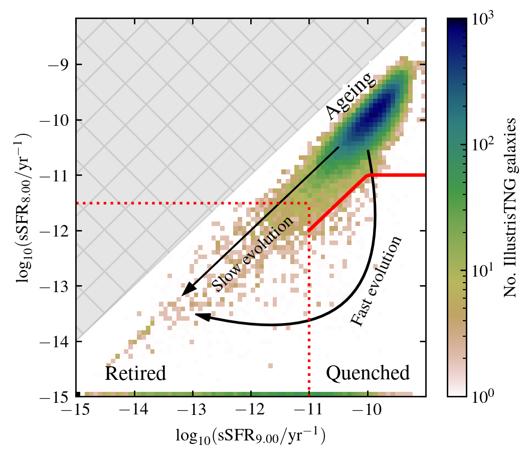
Figure 1: Distribution of IllustrisTNG galaxies across the plane defined by the average specific star-formation measured over the last $10^{8}$ (${\rm sSFR}_{8}$) and $10^{9}$ yr (${\rm sSFR}_{9}$). Quenched galaxies are found below the red solid line, whereas the dotted line delimits the Retired domain. Ageing systems are located above both regions. The grey-shaded area denotes the forbidden region of the parameter space.

The division between Retired galaxies and the other regions is set by the observational limit where specific star formation rates can be reliably measured. Retired galaxies exhibit extremely low ${\rm sSFR}_{\tau}$ values at both timescales, making it challenging to distinguish between systems that underwent quenching events more than one Gyr ago, and those that secularly evolved without any significant suppression of star formation. In the simulations, substituting the mass resolution into Eq. (3) yields the minimum stellar mass of an IllustrisTNG Retired galaxy

$$M_{\rm min}=\frac{\rm SFR_{8,\,min}}{{\rm sSFR}_{8}(\rm RGs)}=\frac{1.4\times 10^{6}\,{M_{\odot}}/10^{8}\,{\rm yr}}{3\times 10^{-12}\,{\rm yr^{-1}}}\approx 5\times 10^{9}{M_{\odot}}.$$ (4)

3.2 Bayesian inference of physical parameters

The values of ${\rm sSFR}_{\tau}$ of Illustris-TNG and Euclid galaxies are inferred from their synthetic and observed fluxes using BESTA (Bayesian Estimator for Stellar Population Analysis, Corcho-Caballero et al., in prep.), a Python-based Bayesian framework for deriving physical properties from observational data. BESTA integrates the PST (Population Synthesis Toolkit), and CosmoSIS (Cosmological Survey Inference System, Zuntz et al. 2015) libraries devoted for highly flexible stellar population synthesis, and Monte Carlo sampling techniques, respectively.

PST is designed to provide a user-friendly interface for working with simple stellar population (SSP) models and synthesizing a variety of observable quantities such as spectra or photometry from different prescriptions of the star-formation and chemical enrichment histories. On the other hand, CosmoSIS is a framework, originally devoted for cosmological parameter estimations, that brings together a wide diversity of Bayesian inference methods in a modular architecture.

We infer the values of ${\rm sSFR}_{\tau}$ by describing the star formation history of galaxies using a non-analytic model. The fraction of the total stellar mass formed by cosmic time $t$, denoted as $\widetilde{M}_{\ast}(t)\equiv M_{\ast}(t)/M_{\ast}(t_{\rm obs})$, where $t_{\rm obs}$ is the age of the Universe at the time of observation, is parametrised as a monotonic piecewise function, with boundary conditions $\widetilde{M}_{\ast}(0)=0$ and $\widetilde{M}_{\ast}(t_{\rm obs})=1$. This function is related to ${\rm sSFR}_{\tau}$ (Eq. 1) by the expression

$$\widetilde{M}_{\ast}(t_{\rm obs}-\tau)=1-\tau\,{\rm sSFR}_{\tau}$$ (5)

During the sampling, Eq. (5) is evaluated at fixed lookback times $\tau\equiv t_{\rm obs}-t=0.1$, 0.3, 0.5, 1, 3, and 5 Gyr. The values of $\tau$ are chosen to roughly align with the age ranges where SSPs exhibit the largest differences in optical/IR colours (Millán-Irigoyen et al. 2021). The values of ${\rm sSFR}_{\tau}$ are sampled from a log-uniform prior distribution within $-14<\log_{10}({\rm sSFR}_{\tau}/\mathrm{yr}^{-1})<1/\tau$, for each value of $\tau$, rejecting solutions that do not yield a monotonically increasing $\widetilde{M}_{\ast}(t)$. For each sample of ${\rm sSFR}_{\tau}$, we estimate $\widetilde{M}_{\ast}(t)$ by interpolating the 8 points (six values of $\tau$ + boundary conditions) using a monotonic cubic spline.

The chemical evolution of the stellar content of galaxies is modelled by assuming that the metallicity of stars formed at a given time, $Z(t)$, is proportional to the mass growth history of the galaxy, following

$$Z(t)=Z(t_{0})\,\frac{M_{\ast}(t)}{M_{\ast}(t_{0})}=Z(t_{0})\,\widetilde{M}_{\ast}(t),$$ (6)

where $Z(t_{0})$, the metallicity of stars formed at $t_{0}$, is sampled using a uniform prior distribution between $0.25<Z(t_{0})/Z_{\odot}<4$. For the sake of clarity, Eq. (6) is related to the mass-weighted average stellar metallicity, $Z_{\ast}$, by the expression

$$Z_{\ast}(t_{0})\equiv\frac{\int_{0}^{t_{0}}\,{\rm SFR}(t^{\prime})\,Z(t^{\prime})\,{\rm d}t^{\prime}}{\int_{0}^{t_{0}}\,{\rm SFR}(t^{\prime})\,{\rm d}t^{\prime}}=\frac{Z(t_{0})}{2}.$$ (7)

To build composite spectra and associated photometric fluxes resulting from the model described above, $\widetilde{M}_{\ast}(t)$ and $Z(t)$ are evaluated at the grid edges defined by the PyPopStar SSPs (Millán-Irigoyen et al. 2021, see Sect. 2.2 for more details). This allows us to estimate the relative contribution of each SSP, $\widetilde{M}_{\rm SSP}(t,Z)$ for any given SSP age and metallicity, and the resulting spectral energy distribution (SED), in units of specific luminosity per wavelength unit and stellar mass, is computed as:

$$L_{\lambda}(\lambda)=\sum L_{\rm SSP}(t,Z,\lambda)\,\widetilde{M}_{\rm SSP}(t,Z).$$ (8)

where $L_{\rm SSP}$ denote the SSP model SEDs.

Dust extinction is included by assuming a single dust screen, using the Cardelli et al. (1989) extinction law with a fixed value of $R_{V}=3.1$. The extinction values given by $A_{V}$, are also sampled from a uniform distribution ranging from 0 to 3.0 mag.

Finally, the predicted specific flux per frequency unit on each photometric band, $\hat{f}_{\nu,i}$, is given by the expression

$$\begin{split}\hat{f}_{\nu,i}=\frac{\int_{0}^{\infty}10^{-0.4\,A_{V}}\,F_{\lambda}\left[\lambda\,\left(1+z\right)^{-1}\right]\,S_{i}(\lambda)\,\lambda\,{\rm d}\lambda}{\int_{0}^{\infty}\frac{3631{\rm Jy}}{c\,\lambda}S_{i}(\lambda)\,{\rm d}\lambda},\\ F_{\lambda}\left[\lambda\,\left(1+z\right)^{-1}\right]=\frac{L_{\lambda}\left[\lambda\,\left(1+z\right)^{-1}\right]}{(1+z)\,4\pi d_{\rm L}^{2}},\end{split}$$ (9)

where $S_{i}$ is the transmission function of the filter $i$, $z$ is the source redshift, and $d_{\rm L}$ is the luminosity distance evaluated at $z$.

Given a set of flux measurements, $f_{\nu,i}$, and assuming Gaussian uncertainties, the log-likelihood associated to a given model can be computed as

$$\ln\mathcal{L}(f|\theta)=\sum_{i}-0.5\left(\frac{f_{\nu,i}-\alpha\,\hat{f}_{\nu,i}}{\sigma(f_{\nu,i})}\right)^{2},$$ (10)

where $\theta$ denotes the vector of parameters used in the model, $\alpha$ is a normalisation constant between the observed and the predicted fluxes that corresponds to $M_{\ast}(t_{0})$, computed using the mean value of $f_{\nu,i}/\hat{f}_{\nu,i}$, and $\sigma(f_{\nu,i})$ represent the flux uncertainty estimates associated to each band $i$.

Given a prior, $P\left(\theta\right)$, Bayes’ theorem determines that the posterior probability distribution of a given model, $P\left(\theta|f\right)$, can be estimated as

$$P\left(\theta|f\right)=\frac{\mathcal{L}\left(f|\theta\right)\,P\left(\theta\right)}{\int\mathcal{L}\left(f|\theta\right)\,P\left(\theta\right){\rm d}\theta}\propto\mathcal{L}\left(f|\theta\right)\,P\left(\theta\right),$$ (11)

where the denominator denotes the Bayesian evidence, that for the purposes of this work can be simply treated as a proportionality constant.

To efficiently explore the posterior probability distribution, we use the max-like and emcee (Foreman-Mackey et al. 2013) samplers available in CosmoSIS. The former performs an initial minimisation of the problem, trying to locate the maximum of the posterior distribution, whereas the second sampler is a form of Monte-Carlo Markov chain that uses an ensemble of walkers to explore the parameter space. The resulting chain of parameters values are used to estimate the 9-dimensional posterior PDF via a Gaussian kernel density estimator (KDE) and derive the percentile values of ${\rm sSFR}_{\tau}$, $Z(t_{0})$, $A_{V}$, and $M_{\ast}(t_{0})$. The parameters used in the modelling of the observed photometry and associated priors are summarised in Table 1. The redshift is fixed to the spectroscopic measurement, and stellar masses are based on the $\Lambda$CDM luminosity distance. Note that the latter factor does not affect the sSFR.

Table 1: Parameters used in BESTA for the SFH inference.

Parameter	Prior	Description
$\log_{10}({\rm sSFR}_{8.00}/\rm yr^{-1})$	unif($-14$, $-8.00$)	Last 0.10 Gyr
$\log_{10}({\rm sSFR}_{8.48}/\rm yr^{-1})$	unif($-14$, $-8.48$)	Last 0.3 Gyr
$\log_{10}({\rm sSFR}_{8.70}/\rm yr^{-1})$	unif($-14$, $-8.70$)	Last 0.5 Gyr
$\log_{10}({\rm sSFR}_{9.00}/\rm yr^{-1})$	unif($-14$, $-9.00$)	Last 1 Gyr
$\log_{10}({\rm sSFR}_{9.48}/\rm yr^{-1})$	unif($-14$, $-9.48$)	Last 3 Gyr
$\log_{10}({\rm sSFR}_{9.70}/\rm yr^{-1})$	unif($-14$, $-9.70$)	Last 5 Gyr
$A_{V}$	unif(0.0, 2.5)	Dust extinction
$Z(t_{0})$	unif(0.005, 0.08)	Present metallicity

4 Results

4.1 Accuracy of the sSFR estimates

First, we utilise the results obtained from fitting IllustrisTNG synthetic photometry to benchmark the reliability of recovering the correct values of ${\rm sSFR}_{\tau}$. In order to minimise the impact of catastrophic outliers, we remove from our sample those galaxies with a poor fit quality. This is done by comparing the maximum value of the posterior probability distribution of each galaxy with the total distribution. We discard sources with values lower than the 5th percentile of the distribution (i.e., 5% of the total sample). Although no clear correlation is observed between the physical properties of the galaxy sample and the fit results, we find that fits fail more frequently for galaxies with high extinction ($A_{V}>0.8$).

Figure 2: IllustrisTNG ${\rm sSFR}_{\tau}$ true values versus the median value recovered by BESTA. Coloured maps denote the number of sources in each bin. Bottom to top red lines of every panel correspond to the running 5, 50, and 95 percentiles of ${\rm sSFR}_{\tau}$ as function of the true value. Dashed and dotted black lines illustrate the one-to-one and 0.5 dex offset lines, respectively. Each panel includes at the top-right corner the fraction of sources whose true value lies within the 68 and 90% estimated credible intervals, respectively.

The true input values of ${\rm sSFR}_{\tau}$ versus the median value recovered by BESTA are shown in Fig. 2, for the combined sample that includes the realisations at $z=0.0$, $0.3$, and $0.6$ (see Appendix B for plots at each redshift bin). For any true value of ${\rm sSFR}_{\tau}$, the red lines denote the 5th, 50th, and 95th running percentiles of the median ${\rm sSFR}_{\tau}$ retrieved by BESTA, illustrating where the bulk of the distribution lies. Overall, the results are satisfactory across all timescales ($\tau$), although we notice some systematic bias. For short timescales (top row panels), BESTA occasionally underestimates the true value of ${\rm sSFR}_{\tau}$, leading to an artificial population of galaxies with ${\rm sSFR}_{8/8.48}\simeq 10^{-14}\,\rm yr^{-1}$. Conversely, when the true value is consistent with 0, i.e. no stellar particle was formed in the last $\tau$ Gyr (artificially set to ${\rm sSFR}=10^{-15}\,\rm yr^{-1}$ for visualisation purposes), the inferred median values typically stay close to the prior limit at $10^{-14}\leavevmode\nobreak\ \rm yr^{-1}$, but they also present an extended tail towards higher values of ${\rm sSFR}_{\tau}$ up to about $10^{-11}\leavevmode\nobreak\ \rm yr^{-1}$. This clearly highlights how difficult is to distinguish between strictly 0 and the $\simeq 1\%$ level in terms of the mass fraction formed over a given timescale using optical/IR photometry (e.g., Salvador-Rusiñol et al. 2020).

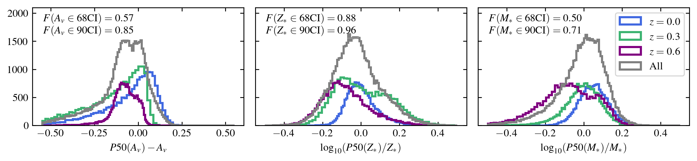
Figure 3: Statistical distribution of the difference between the input IllustrisTNG values of dust extinction, $A_{V}$, stellar metallicity $\log_{10}(Z_{\ast}/Z_{\odot})$, and total stellar mass, $\log_{10}(M_{\ast}/\rm{M_{\odot}})$, versus the median value recovered by BESTA. Each panel includes the fraction of sources whose true value lies within the 68 and 90% estimated credible intervals, respectively.

At longer timescales ($\tau>1$ Gyr), BESTA tends to overestimate ${\rm sSFR}_{\tau}$ for values below $10^{-11}\leavevmode\nobreak\ \rm yr^{-1}$. The resulting median values typically lie in the range $10^{-12}$–$10^{-10}\leavevmode\nobreak\ \rm yr^{-1}$, which corresponds to formed mass fractions of $0.003$–$0.3$ and $0.005$–$0.5$ at lookback times of 3 and 5 Gyr, respectively, in contrast to the true value of 0. In general, we observe that extreme outliers, i.e., that values significantly above/below the one-to-one line, primarily emerge as a consequence of over/under-estimating the dust extinction and/or metallicity by approximately $\gtrsim 0.2$ dex.

Given the intrinsic degeneracy between the parameters of our model, that may lead to an erroneous classification, it is of the utmost importance to not only rely on the median/mean/mode estimates of the resulting posterior PDF, but to make use of the whole distribution to account for the large uncertainties. To that end, Fig. 2 also includes the fraction of sources whose real value of ${\rm sSFR}_{\tau}$ lies within the 68 and 90% credible intervals estimated from the posterior PDF. This number depends on how well-calibrated the credible intervals are to the actual posterior probabilities and can be used as a proxy of the ability of the model to capture the complexity of the data. To estimate the fractions, only sources with ${\rm sSFR}_{\tau}>10^{-14}\leavevmode\nobreak\ \rm yr^{-1}$ have been considered. As expected from a reasonably well-calibrated estimate of the uncertainties associated to ${\rm sSFR}_{\tau}$, both intervals properly account for $\simeq 68$% and $\simeq 90$% of the sample.

In Fig. 3, we show the ratio between the median value of the other physical properties included in the model – dust extinction, $A_{V}$, stellar metallicity $\log_{10}(Z_{\ast}/Z_{\odot})$, and total stellar mass, $\log_{10}(M_{\ast}/\rm{M_{\odot}})$ – and the true input value, for the three samples considered in this work (at $z=0$, $0.3$, and $0.6$, respectively). The three quantities are roughly recovered by BESTA with a reasonable degree of accuracy (about $0.2$ dex), although the biggest challenge is to effectively inferring $A_{V}$. In a significant fraction of cases, $A_{V}$ is underestimated, resulting into an increase of the metallicity for compensating the change of colours. As a result of changing the mass-to-light ratio of the underlying stellar population, the final stellar mass estimate is also affected by a few per cent. Nevertheless, the posterior probability distribution still seems to properly account for the intrinsic uncertainties as indicated by the fraction of sources within the 68 and 90 credible intervals.

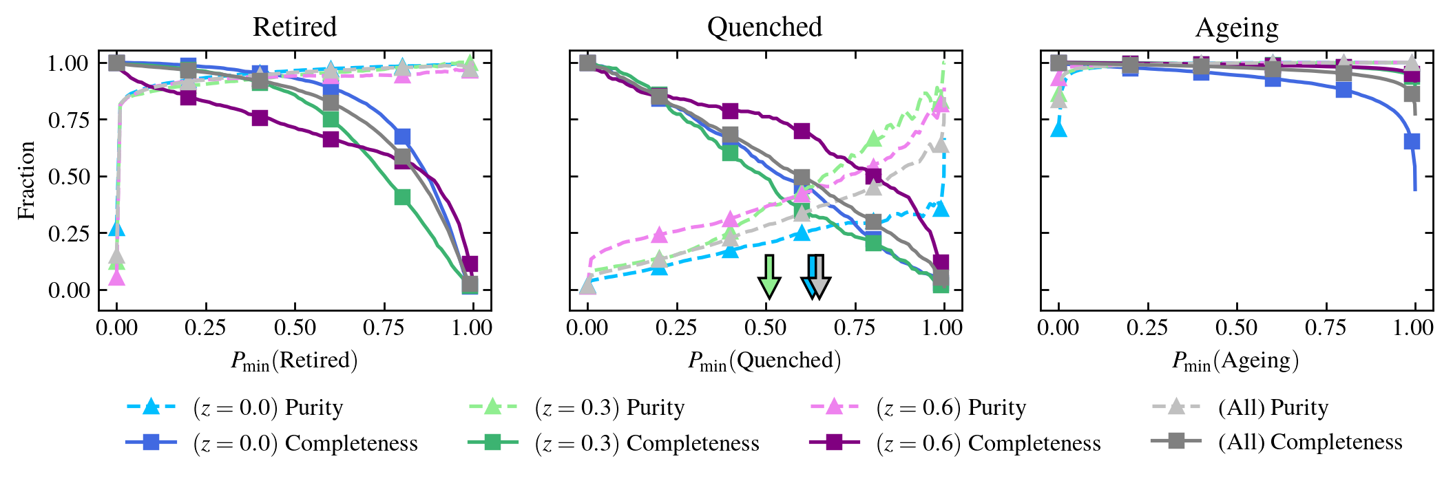
Figure 4: Retired (left), Quenched (middle), and Ageing (right) galaxy classification purity and completeness, as function of the minimum probability threshold used to perform the classification. Each redshift sample at $z=0$, $z=0.3$, and $z=0.6$ is denoted by the blue, green, and purple lines, respectively. Coloured arrows denote the value of $P_{\rm min}(\rm Quenched)$ that maximises the $F$-score at each redshift (see Sect. 4.3).

It is worth remarking that the use of the median value is adopted only for its simplicity in terms of visualisation purposes. Throughout the remaining sections the goal is to make use of the entire posterior PDF in order to maximise the information content. In addition, it is also important to point out that our fitting procedure assumes the same basic ingredients (IMF, SSPs, extinction law) as the mock observations. This is of course an ideal case, and therefore our estimated uncertainties should be regarded as a lower limit (see e.g., Conroy 2013, for an exhaustive discussion).

4.2 Probabilistic AD classification

In this section we present our classification scheme mainly devoted for discriminating between slow (Ageing) and fast (Quenching) evolution. Here, we describe the method based on analysing the posterior probability distribution of each galaxy. In contrast, Sect. 4.4 introduces an alternative, model-driven approach that maximises classification completeness and purity by leveraging the predictive power of the IllustrisTNG simulation.

We estimate the probability that a galaxy belongs to the Ageing, Quenched and Retired populations ($i$) by integrating the marginalised posterior PDF, $P({\rm sSFR}_{9},{\rm sSFR}_{8}|f)$, over the regions $D(i)$ defined by the AD classification (described in Sect.  3.1), as specified by Eqs. (2) and (3)

$$P(i)=\frac{\iint_{D(i)}P({\rm sSFR}_{9},{\rm sSFR}_{8}|f)\,{\rm d}\log_{10}\left(\frac{{\rm sSFR}_{9}}{\rm yr^{-1}}\right)\,{\rm d}\log_{10}\left(\frac{{\rm sSFR}_{8}}{\rm yr^{-1}}\right)}{\int P(\theta|f)\,{\rm d}\theta},$$ (12)

where the denominator represents the Bayesian evidence for the model, and $P(i)$ indicates the probability of the galaxy being classified as Ageing, Quenched, or Retired, and $\sum P(i)=1$.

In Fig. 4 we show the purity and completeness fraction achieved when classifying the Retired (left), Quenched (middle), and Ageing (right) populations by imposing a minimum probability threshold, $P_{\rm min}$, on the sample of IllustrisTNG galaxies. For each class, purity and completeness are defined as the number of true positives divided by the total number of observed (true and false) positives, $N_{\rm TP}/(N_{\rm TP}+N_{\rm FP})$, and the ratio between true positives divided by the number of true positives and false negatives, $N_{\rm TP}/(N_{\rm TP}+N_{\rm FN})$, respectively. To explore the effects of redshift on the performance of the classification, the sample has been split into the three redshift bins under consideration: $z=0.0$, $0.3$, and $0.6$. Both Ageing and Retired populations are successfully classified with purity scores above 80% at all redshift bins. The completeness of both classes presents a stronger dependence with redshift. For a given probability threshold, retired galaxies tend to be more under-represented at higher values of $z$, whereas constraining the fraction of Ageing systems at $z\simeq 0$ results more challenging than at high redshift.

On the other hand, estimating the population of Quenched galaxies presents more difficulties. At $z=0$, the population of Quenched galaxies is poorly identified, and it includes a significant number of false positives, that strongly limit the purity of the sample to $\simeq 30\%$ even when applying a threshold cut of $P_{\rm min}({\rm Quenched})>0.75$. When considering the same cut at higher values of $z$, this bias is significantly alleviated, and the sample purity increases to values between 50% and 75%. This is expected since optical photometry becomes more sensitive to the recent star-formation episodes due to the more prominent contribution of rest-frame UV light (mostly supported by young stellar populations).

4.3 Selection of quenched galaxies

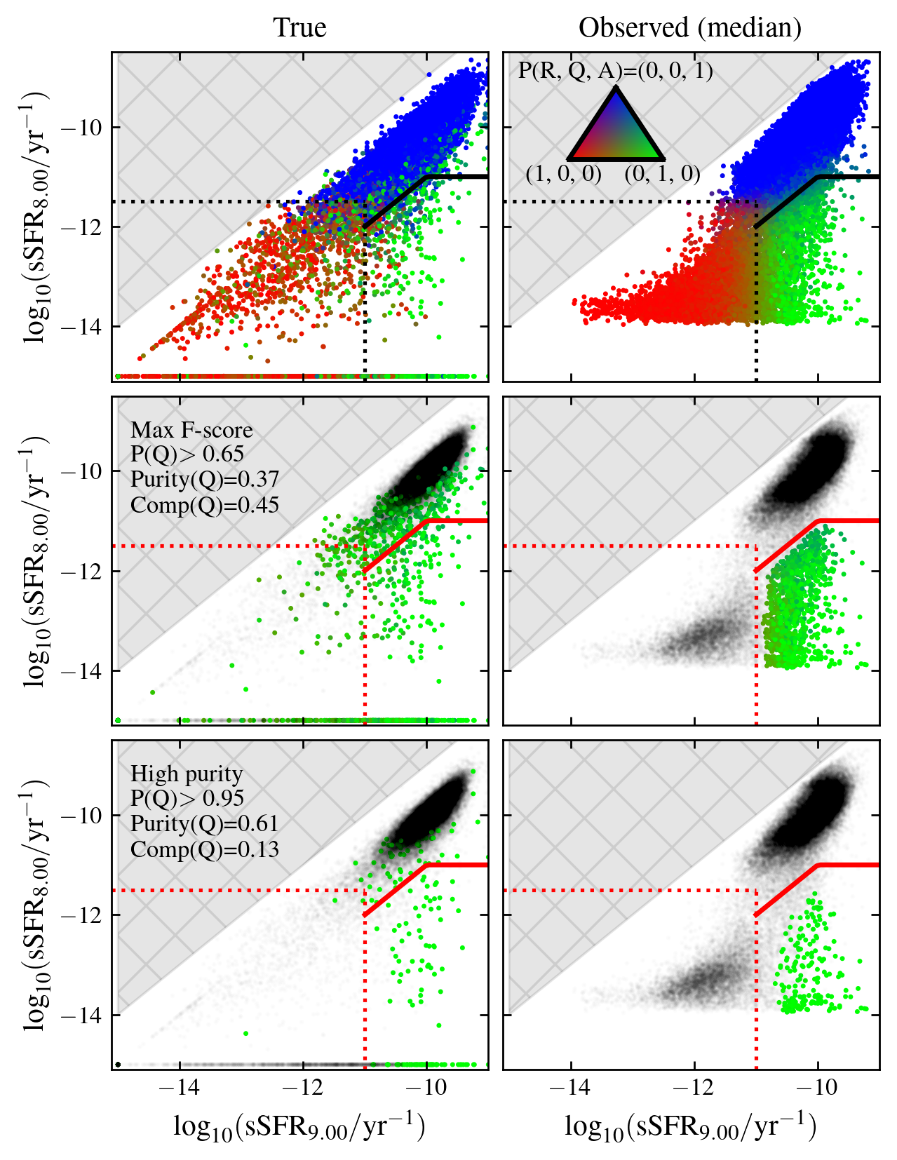
Figure 5: Distribution of IllustrisTNG galaxies across the ${\rm sSFR}_{9}$ versus  ${\rm sSFR}_{8}$ plane. Left and right columns show the distribution based on the true (null values of ${\rm sSFR}$ are arbitrarily set to $\log_{10}({\rm sSFR}/\rm yr^{-1})=-15$) and inferred median values, respectively. Top row panels display the full sample RGB colour-coded by the probability of belonging to the Retired, Quenched, and Ageing classes. Solid and dotted lines represent the demarcation lines given by Eqs. 2 and 3, respectively. Middle and bottom rows illustrate the two proposed approaches for selecting quenched galaxies (coloured points) by colouring in black with low transparency those systems classified as Retired or Ageing.

In this section, we present two approaches for selecting quenched galaxies, each tailored to different priorities in classification performance. The first approach emphasises a balance between purity and completeness, achieved by selecting the probability threshold $P_{\rm min}(\rm Quenched)$ that maximises the $F$-score, defined as

$$F=\frac{2N_{\rm TP}}{2N_{\rm TP}+N_{\rm FP}+N_{\rm FN}},$$ (13)

where $N_{\rm TP}$, $N_{\rm FP}$, $N_{\rm TN}$, and $N_{\rm FN}$ represent the number of true positives, false positives, true negatives, and false negatives, respectively.

From the purity and completeness values shown in Fig. 4, we determine the optimal $P_{\rm min}(\rm Quenched)$ values for the samples at $z=0.0$, $0.3$, and $0.6$ to be 0.63, 0.51, and 0.65, respectively. When combining the three redshift samples, the optimal threshold becomes $P_{\rm min}(\rm Quenched)=0.65$, yielding a combined purity of 37% and a completeness of 45%.

The second approach prioritises maximizing the purity of the quenched galaxy sample, even at the expense of low completeness. For this, we adopt a stricter threshold, $P_{\rm min}(\rm Quenched)=0.95$. This choice results in sample purities of 35%, 86%, and 76% at $z=0.0$, $0.3$, $0.60$, respectively, with a combined purity fraction of 61%.

To evaluate the performance of these classification schemes, Fig. 5 displays the true (left) and median-based (right) distribution of IllustrisTNG galaxies across the ${\rm sSFR}_{9}$ versus ${\rm sSFR}_{8}$ plane. In the top row, all galaxies are colour-coded according to their probabilities of belonging to the Retired, Quenched, and Ageing domains using an RGB palette.

The ‘balanced’ classification approach, which maximises the $F$-score, is illustrated in the middle row. Here, Retired and Ageing galaxies are shown in semi-transparent black to emphasise the spatial distribution of quenched systems. As can be readily seen, this method misclassifies a significant fraction of Ageing systems located below the main sequence (MS) locus, roughly centred at $\log_{10}\left({\rm sSFR}_{8,\,9}/\rm yr^{-1}\right)\approx-10$. In addition, there is also a small fraction ($\simeq 3\%$) of contaminants with very low values of ${\rm sSFR}_{9}$.

The classification that maximises sample purity is shown in the bottom row. This method significantly reduces contamination, with the remaining misclassified systems primarily consisting of Ageing galaxies with moderate to low star-formation rates. Overall, the selected population of Quenched galaxies is now dominated by systems with higher values of ${\rm sSFR}_{9}$, implying a more vigorous star-forming activity in the past compared to the current rate. These systems fall closer to the ‘post-starburst’ definition: galaxies with strong stellar Balmer absorption, due to the preponderance of A-type stars, and very little to null nebular emission, indicative of the demise of O- and B-type stars, implying a quenching event that truncated star-formation after the burst of star-formation. However, the biggest drawback of this classification is its low completeness, only reaching values close to 10%. Nevertheless, the vast cosmological volume probed by Euclid will alleviate this problem by providing an immense wealth of galaxies.

4.4 Model-driven classification

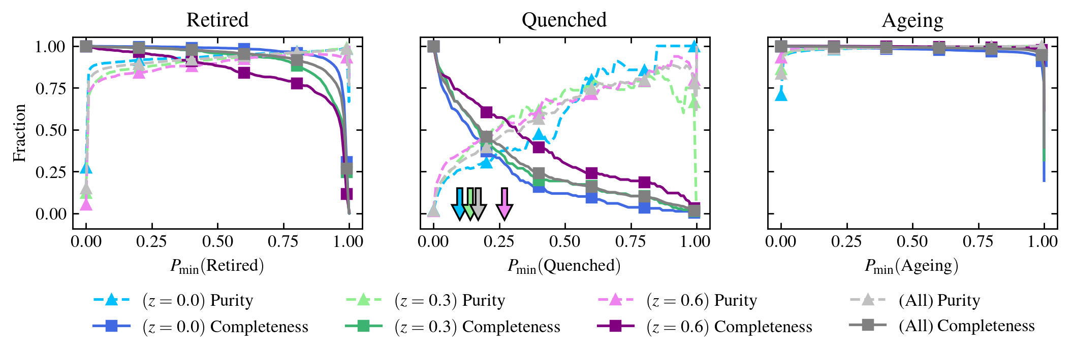
Figure 6: Same as Fig. 4, using the classification presented in Sect. 4.4.

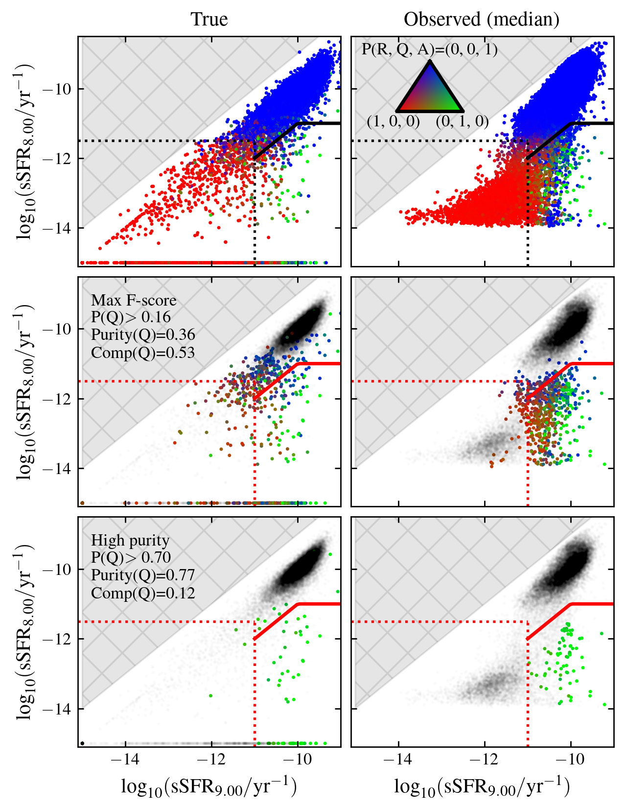
Figure 7: Same as Fig. 5, using the classification presented in Sect. 4.4.

The classification method presented in the previous section relies on a marginalised version of the posterior, constrained to the space defined by ${\rm sSFR}_{9}$ and ${\rm sSFR}_{8}$. While this approach is appealing due to its simplicity and ease of interpretation, the full posterior, $P({\rm sSFR}_{\tau}|f)$, contains significantly richer information that can be used to refine the classification. To this end, we have estimated the probability distribution, defined in terms of the 5th, 16th, 50th, 84th, and 95th percentiles of ${\rm sSFR}_{\tau}$, with $\log_{10}(\tau/{\rm yr})=\{8.00,\,8.48,\,8.70,\,9.00\}$, along with the correlation coefficients computed from the covariance matrix, $\rho\left({\rm sSFR}_{\tau_{1}},{\rm sSFR}_{\tau_{2}}\right)$, for the population of Ageing, Quenched and Retired galaxies, respectively. This distribution is more sensitive to subtle differences between the three populations, and can enhance the reliability of the classification.

To properly handle the 26-dimensional parameter space, denoted by the vector $\theta$, we have used a Gaussian KDE. We denote the PDF associated to each AD class, $i$, as ${\rm KDE}_{i}(\theta)$. To classify individual objects, we compute the probability of the galaxy being drawn from the Ageing, Quenched, or Retired distribution. The probability of belonging to each class is computed as

$$P_{{\rm KDE},\,i}(\theta)=\frac{{\rm KDE}_{i}(\theta)}{{\sum_{{i}\in\{\rm A,\,Q,\,R\}}{\rm KDE}_{i}(\theta)}}.$$ (14)

The training process uses 80% of the total sample, randomly selected, while the remaining 20% forms the test sample to assess classification performance. The kernel bandwidth is optimised to maximise the mean classification score across all three classes and fixed to 0.38. Figure 6 presents the resulting purity and completeness scores for the test sample, demonstrating an improvement compared to the results in Fig. 4. For Ageing and Retired systems, purity and completeness exhibit reduced sensitivity to the threshold $P_{\rm min}$, and are systematically higher across all cuts. For quenched galaxies, the most significant improvement lies in the increase in purity across all redshift bins, nearly doubling for the $z=0$ sample. However, completeness decreases consistently, falling below 30% for $P_{\rm KDE,\,min}(\rm Quenched)\geq 0.5$.

Figure 7 illustrates the application of the KDE-based classification method, analogous to Fig. 5. The number of false positives classified as quenched systems is significantly reduced, but this improvement comes at the cost of a smaller sample size and lower completeness. For the KDE method, the threshold $P_{\rm KDE,\,min}(\rm Quenched)=0.16$ maximises the $F$-score, achieving purity and completeness values of 36% and 53%, respectively, which is a marginal improvement over the criteria proposed earlier. However, as shown in the middle-row panels, many selected sources exhibit higher probabilities of being classified as Ageing or Retired systems.

On the other hand, this method excels the previous one when selecting a high-purity sample. A stricter cut of $P_{\rm KDE,\,min}(\rm Quenched)\geq 0.7$, shown in the bottom panels, achieves a purity of 77%, and completeness of 12%. This represents an improvement over the previous results, which yielded a purity and completeness of 61% and 13%, respectively.

While the KDE-based classification significantly enhances the identification of quenched systems, this improvement is strongly influenced by the training data. The classification depends on the star-formation histories of IllustrisTNG galaxies, the recipes used to generate the synthetic observables (PyPopStar, PST) and the recovery of physical properties using (BESTA). Careful validation is necessary when applying this method to other data sets to ensure its robustness.

4.5 Ageing and Quenching in Euclid

Figure 8: Top: Distribution of Euclid galaxies across the stellar mass versus ${\rm sSFR}_{8}$ plane. The dotted line denotes the definition of the SFMS by Popesso et al. (2023). Bottom: Distribution of Euclid galaxies across the ${\rm sSFR}_{9}$ versus ${\rm sSFR}_{8}$ plane. The dotted and solid lines denote the Retired and Quenched domain demarcation lines.

Here we apply the classification methods described in the previous Sects. 4.2 and 4.4 to our sample of Euclid galaxies, based on the results inferred using BESTA (see Sect. 3.2). The distributions and fractions presented in this section are volume-corrected, accounting for the sample selection effects described in Appendix A.

The top row of Fig. 8 illustrates the distribution of galaxies across the plane defined by their inferred (median) total stellar mass and ${\rm sSFR}_{8}$ across multiple redshift bins. The location of galaxies along the star-forming main sequence aligns reasonably well with previously reported values in the literature (e.g., Popesso et al. 2023) and the recent findings of Euclid Collaboration: Enia et al. (2025). In terms of mass completeness, dwarf galaxies with stellar masses below $10^{9}\leavevmode\nobreak\ {M_{\odot}}$ are detected only in the lowest redshift bin ($z\leq 0.1$). Galaxies in the mass range ($10^{9}\leq M_{\ast}/\,{M_{\odot}}\leq 10^{10}$) are observed up to redshift of approximately $0.4$, while massive systems ($M_{\ast}\geq 3\times 10^{10}\,{M_{\odot}}$) are detected over the whole redshift range.

In terms of star-forming activity, galaxies with stellar masses above $M_{\ast}\gtrsim 10^{10.5}\,{M_{\odot}}$ generally exhibit very low ${\rm sSFR}_{8}$ values, often corresponding to upper limits. Conversely, the fraction of low-mass systems below the main sequence increases at lower redshifts.

The bottom row of Fig. 8 presents the distribution of galaxies across the ${\rm sSFR}_{9}$ versus ${\rm sSFR}_{8}$ plane. This parameter space offers a complementary view to the $M_{\ast}$–${\rm sSFR}_{8}$ plane, offering additional insights into the current evolutionary states of galaxies. A well-defined sequence of ageing galaxies is observed, characterised by roughly constant ${\rm sSFR}$ values over the past Gyr, ranging from $3\times 10^{-12}$ to $10^{-9}\,\rm yr^{-1}$, across all redshift bins. Additionally, a distinct population of quenched galaxies, recently detached from the ageing sequence, is detected. These two evolutionary pathways converge in the lower-left region of the diagram, forming a population of retired galaxies, with minimal star formation, whose light is completely dominated by old stellar populations.

The top-left corner of each panel indicates the volume-corrected fractions of Ageing, Quenched, and Retired galaxies (see Fig. 13 for details about the sample completeness in terms of RGs), labelled using the posterior and KDE-based classification schemes with cuts that maximise the $F$-score (see Sects. 4.3 and 4.4). The results from the two classifiers are consistent across all redshift bins. Ageing galaxies consistently dominate the population, representing over $70\%$ in all bins. Quenched galaxies become increasingly prevalent at lower redshifts, while the fraction of retired systems grows from $8$–$10$ up to $15$–$25\%$. However, these trends are also affected by sample selection effects, since low-mass Quenched and Retired galaxies become more difficult to detect at high $z$ (see Sect. 5.1 for further discussion).

To contextualise these findings, we compare the fractions in the lowest redshift bin ($0.01<z<0.1$), where the sample is complete up to about $10^{9}\,{M_{\odot}}$, with the results reported in CC23a. The authors estimated volume-corrected fractions of Ageing, Quenched, and Retired galaxies, using both IllustrisTNG and the MaNGA survey (Bundy et al. 2015), based the $\rm EW(\mathrm{H}\alpha)$ versus $D_{n}(4000)$ Ageing Diagram. Table 2 summarises this comparison, listing the total fractions of these populations derived from the Euclid and IllustrisTNG samples (the latter using the realisation at $z=0$). The fractions were computed with both the Bayesian posterior and KDE-based classifiers, employing three criteria: the minimum probability threshold ($P_{\rm min}$) that maximises the $F$-score; the threshold maximizing purity; and the label with the highest probability. This results in six fraction estimates for each sample.

Table 2: Comparison of the fractions of Retired (RG), Quenched (QG), and Ageing (AG) galaxies at $z<0.1$ for the Euclid and IllustrisTNG samples with results from CC23a. Fractions are estimated using Bayesian posterior and KDE-based classification schemes under three criteria: minimum probability threshold ($P_{\rm min}$) that maximises $F$-score, threshold maximizing purity, and label with the highest probability. For IllustrisTNG, fractions are also provided using the true values of ${\rm sSFR}_{8}$ and ${\rm sSFR}_{9}$.

Data set and Method	F(RGs)	F(QGs)	F(AGs)
Euclid ($z<0.1$)
Post. (max $F$-score)	0.14	0.10	0.68
Post. (high purity)	0.14	0.04	0.68
Post. (max prob.)	0.14	0.17	0.68
KDE (max $F$-score)	0.19	0.08	0.72
KDE (high purity)	0.16	0.13	0.70
KDE (max prob.)	0.19	0.09	0.72
IllustrisTNG ($z=0$)
Truth (true values)	0.27	0.02	0.71
Post. (max $F$-score)	0.26	0.03	0.67
Post. (high purity)	0.26	$<$0.01	0.67
Post. (max prob.)	0.26	0.06	0.67
KDE (max $F$-score)	0.27	0.03	0.70
KDE (high purity)	0.28	$<$0.01	0.70
KDE (max prob.)	0.18	0.04	0.78
CC23a Results
IllustrisTNG	0.23–0.25	0.11–0.14	0.61
MaNGA	0.13–0.15	0.08–0.10	0.72–0.74

Additionally, we can qualitatively compare our results with the star-forming and ‘quiescent’ fractions reported in Euclid Collaboration: Enia et al. (2025), based on the colour-based classification criteria fromWilliams et al. (2009) and Ilbert et al. (2013). For $0.2<z<0.5$, $23\%$ galaxies are classified as quiescent, and the reminder as star-forming. Our findings are in qualitative agreement, with QGs+RGs (AGs) making up 15–17% (82–84%) at $0.2<z<0.4$, and 10–11% (88–89%) in the $0.4<z<0.6$ bin. At higher redshifts ($0.5<z<0.8$), Euclid Collaboration: Enia et al. (2025) find a quiescent fraction of $15\%$ ($85-86\%$ star-forming), whereas we estimate 6–7% QGs+RGs and $93\%$ AGs, most likely driven by the lack of low-mass Quenched and/or Retired systems in our sample (as discussed in Appendix A, our fractions are only representative above $10^{11}\,{M_{\odot}}$ in this redshift bin; cf. Fig. 10 below).

As noted earlier, the two classifiers (Bayesian posterior and KDE) produce consistent results, with more pronounced differences arising between classification criteria, particularly for Ageing and Retired fractions. Overall, there is good qualitative agreement between this work and CC23a. However, when comparing results based on IllustrisTNG, the current analysis yields systematically higher fractions of Ageing galaxies, while the fraction of quenched systems is reduced from 12% to 3%.

Beyond these methodological differences, selection effects and classification biases likely contribute to the observed discrepancies (see Sect. 4.2 for a detailed discussion). Despite these challenges, the comparison with observational data reveals significant agreement, with variations well within the expected systematic uncertainties.

5 Discussion

Understanding the formation mechanisms of galaxies dominated by old stellar populations, with little to no ongoing star formation, become a topic of considerable scientific interest in recent years (e.g., Casado et al. 2015; Quai et al. 2018; Owers et al. 2019; Corcho-Caballero et al. 2021a, 2023b). The detection of such systems at high redshift challenges widely accepted formation models, exposing potential limitations in our cosmological framework (e.g., Girelli et al. 2019; Merlin et al. 2019; Lovell et al. 2023; De Lucia et al. 2024; Lagos et al. 2025). The classification of galaxies into categories such as passive, quiescent, quenched, or, following the nomenclature proposed in Corcho-Caballero et al. (2021b, 2023b, 2023a), retired, remains contentious. This reflects not only the complexity of the varied and intertwined processes that regulate (and potentially halt) star formation, but also the challenges of inferring such low levels of star formation from observational data.

Quiescent galaxies are often identified by imposing sSFR thresholds over specific timescales (Moustakas et al. 2013; Donnari et al. 2019; Tacchella et al. 2022), as well as cuts using proxies of ${\rm sSFR}_{\tau}$ such as broadband colours (e.g., Peng et al. 2010; Schawinski et al. 2014; Weaver et al. 2023). These thresholds are typically calibrated to isolate systems below the star-forming main sequence, with some incorporating redshift evolution (e.g., Tacchella et al. 2022). While this approach has provided valuable insights into galaxy evolution, such as trends in quiescent fractions and their dependence on stellar mass and environment (e.g., Peng et al. 2010; Donnari et al. 2019; Weaver et al. 2023), it often oversimplifies the transition to quiescence by focusing on single timescales and neglecting the diversity of star-formation histories.

To better understand the physical processes that regulate star formation, and quantify their relative contribution, one would need to use more sophisticated classifications than the usual quiescent versus star-forming scenario (e.g., Casado et al. 2015; Moutard et al. 2016, 2018; Quai et al. 2018; Owers et al. 2019; Iyer et al. 2020). In this work, we advocate for a more refined approach, that incorporates multiple timescales to classify galaxies based on their star-formation activity. This methodology captures better the diversity of evolutionary pathways, distinguishing between recently quenched systems and those that have been evolving secularly for longer periods of time.

The discussion is organised as follows. Section 5.1 investigates the dependence of galaxy populations on stellar mass in the Euclid and IllustrisTNG samples in the nearby Universe ($z<0.1$). Section 5.2 explores the evolution of these populations across redshift, highlighting trends within different mass bins.

5.1 Ageing, Quenched and Retired fractions at $z<0.1$

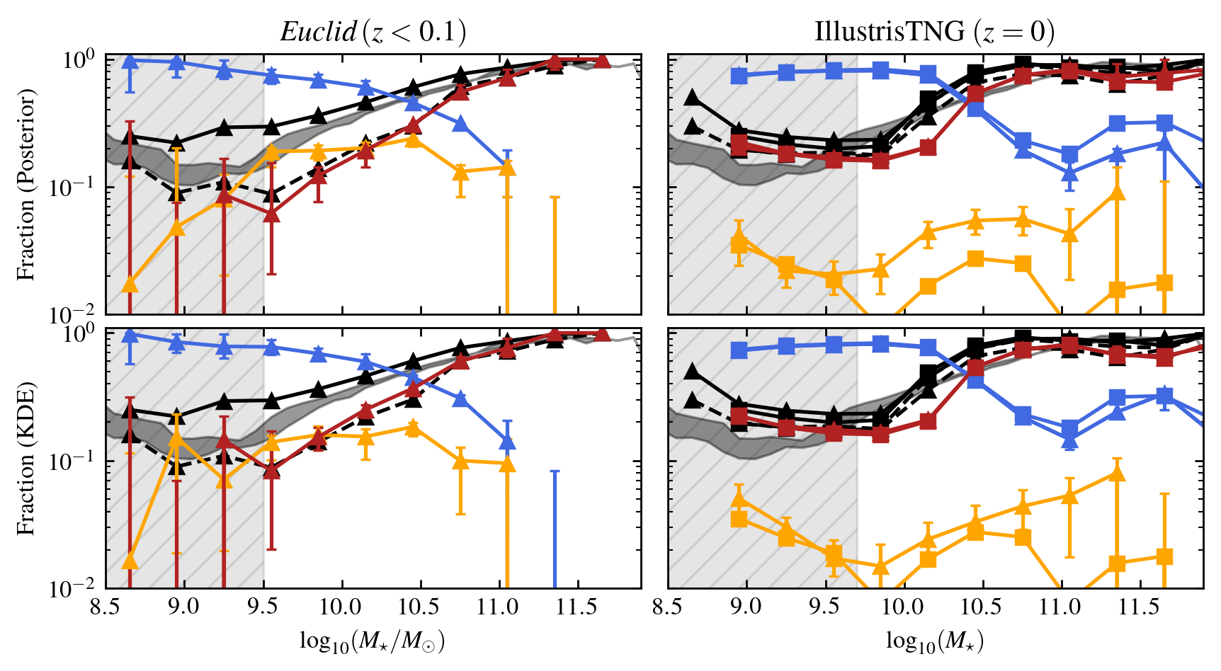
Figure 9: Fraction of galaxies in different classes as function of total stellar mass. Blue, orange and red lines denote the fraction of Ageing, Quenched and Retired galaxies, respectively. Solid and dashed black lines denote the fraction of galaxies with values of ${\rm sSFR}_{8}$ and ${\rm sSFR}_{9}$ below $10^{-11}\,\rm yr^{-1}$. The grey shaded region shows the fraction of galaxies with ${\rm sSFR}\leq 10^{-11}\leavevmode\nobreak\ \rm yr$ (estimated using nebular emission lines and optical photometry) from CC21a. Top and bottom panels make use of the posterior- and KDE-based classification (see Sect. 4.2, and 4.4), respectively. Left panels show the fractions computed using a Euclid sample of nearby galaxies ($z\leq 0.1$), where the grey-hatched area denotes the mass-completeness limit (see Appendix A). The error bars were estimated from 1000 random samples, each selecting 20% of the total sample, and computing the 5 and 95 percentiles. Right panels show the results from the IllustrisTNG sample at $z=0$, including the true values (square symbols), where the grey-hatched area denotes the Retired mass resolution limit (see Sect 3.1).

This section examines the relationship between the fractions of galaxies classified as Ageing, Quenched, or Retired and their total stellar mass. Additionally, we compare our classification methodology to the traditional threshold-based approach that relies on a single average value of sSFR.

Figure 9 presents the fraction of Ageing, Quenched, and Retired galaxies as a function of stellar mass for nearby galaxies ($z<0.1$) in the Euclid (left panels) and IllustrisTNG (right panels) samples. The top and bottom panels compare the two classification schemes outlined in Sects. 4.2 and 4.4, each optimised to maximise the $F$-score. In addition, we include the fractions of galaxies below the star-formation rate threshold of $10^{-11}\,\rm yr^{-1}$ for ${\rm sSFR}_{8}$ and ${\rm sSFR}_{9}$ (solid and dashed black lines, respectively), and compare these with the results of CC21a (grey shaded region), derived from SDSS and GAMA surveys.

The AD classification methods yield highly consistent fractions (coloured lines) for Ageing and Retired galaxies across both Euclid and IllustrisTNG data sets. However, the fraction of Quenched galaxies shows greater sensitivity to the choice of classification method, though the overall trends with stellar mass remain qualitatively similar. In the simulated data (right panels), the true fractions for each class are also included (square symbols). As discussed earlier, the classification tends to slightly overestimate the fraction of Quenched galaxies in IllustrisTNG, particularly at the high-mass end.

A comparison between the two data sets reveals some notable differences. In the IllustrisTNG sample, Retired galaxies dominate at stellar masses $\geq(2$–$3)\times 10^{10}\,\rm{M_{\odot}}$, comprising more than $75$% of the population. Below this threshold, Ageing galaxies dominate, also accounting for over 75% of the population, and the fraction remains nearly constant across these regimes. Observational data from Euclid, however, exhibits a smoother trend with stellar mass. The fraction of Ageing galaxies decreases steadily from approximately 90% of the total sample at the low-mass end towards a negligible value at high masses. In contrast, Retired galaxies show a monotonic increase, reaching around 90% for $M_{\ast}\gtrsim 10^{11}\,\rm{M_{\odot}}$.

The fraction of Quenched galaxies in Euclid remains approximately constant (10–20%) between $3\times 10^{9}$ to $10^{11}\,{M_{\odot}}$, beyond which the fraction drops to null values. The IllustrisTNG sample shows a more intricate structure: while a valley is evident at $M_{\ast}\simeq 10^{10}\,{M_{\odot}}$, an additional dip is observed at even higher stellar masses, around $M_{\ast}\simeq 3\times 10^{11}\,{M_{\odot}}$. Note that, due numerical resolution effects (Sect. 2.2), the IllustrisTNG sample does not accurately probe the galaxy population below $M_{\ast}\simeq 5\times 10^{9}\,{M_{\odot}}$, but we do observe a clear difference between the simulated and observed populations for $M_{\ast}>5\times 10^{9}\,{M_{\odot}}$. While most quiescent galaxies in Euclid are classified as Quenched, they belong to the Retired class in IllustrisTNG.

As previously discussed in CC23b, the choice of timescale for estimating the current star-formation rate significantly impacts the inferred fraction of passive galaxies. For example, when using a longer timescale (e.g., ${\rm sSFR}_{9}$), it yields a steadily increasing fraction of passive galaxies with stellar mass, closely matching the definition of Retired galaxies. In contrast, shorter timescales such as ${\rm sSFR}_{8}$, result in a combined fraction that includes both Quenched and Retired populations, consistent with CC21a.

The observed flat distribution of Quenched galaxies suggests that the quenching mechanism(s), responsible for shutting down star formation on timescales of $\simeq 500$ Myr (CC23a), are equally efficient at all stellar masses, across the range probed by the sample. Conversely, the population of Retired galaxies is primarily populated by massive systems, dominating the fraction of galaxies above $3\times 10^{10}\,{M_{\odot}}$, which can be interpreted in terms of an increase in the impact of internal, and slow, quenching processes such as AGN feedback or virial shock heating, as well as enhanced star formation efficiency (Dekel & Birnboim 2006; Peng et al. 2010; Tortora et al. 2010, 2025). However, these interpretations remain qualitative. A larger sample, more rigorous selection, and expanded analysis are needed to refine these conclusions and further elucidate the physical mechanisms governing galaxy quenching. In summary, our classification provides a rich framework for studying and interpreting the evolutionary trends of galaxies in terms of their recent star-formation history.

5.2 Redshift evolution up to $z=0.8$

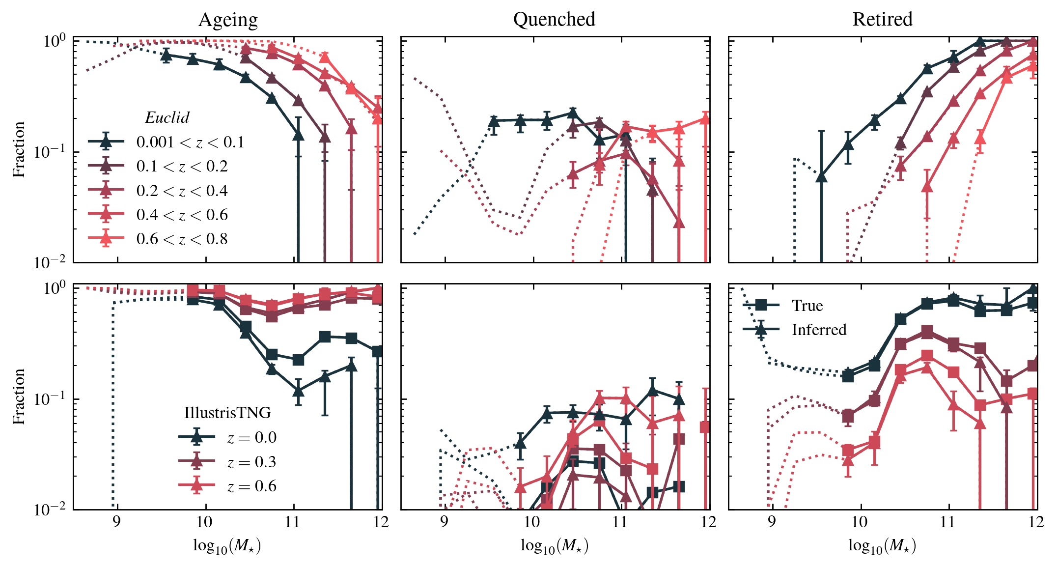
Figure 10: Fraction of Ageing, Quenched and Retired galaxies as function of stellar mass in redshift bins. Each row of panels shows fractions inferred using BESTA for Euclid (top) and IllustrisTNG (middle) samples, along with true fractions from IllustrisTNG (squares). The error bars were estimated from 1000 random samples, each selecting 20% of the total sample, and computing the 5 and 95 percentiles. In the top row, fractions for masses below the mass completeness limit (see Appendix A) are shown as dotted lines. Similarly, in IllustrisTNG, masses below the Retired resolution limit are represented as dotted lines.

Following the results of the previous section, here we examine the evolution of the fraction of each galaxy population as a function of redshift and stellar mass. Figure 10 illustrates the fraction of Ageing (left), Quenched (middle), and Retired (right) galaxies as a function of redshift, divided in bins of stellar mass. The top and bottom rows display the results inferred using BESTA for Euclid and IllustrisTNG samples, including the fractions computed using the true labels of each IllustrisTNG galaxy. The fraction of galaxies in each domain has been computed using the probability estimated from the posterior, adopting the criteria that maximises the $F$-score. The results are rather insensitive to the choice of classifier (i.e., posterior- or KDE-based), presenting only a subtle change on the overall normalisation (see previous section). For the inferred fractions, we have computed qualitative estimates of the Poisson errors by bootstrapping the distribution selecting 1000 random samples and computing the 5th, 50th, and 95th percentiles of the resulting distribution.

In general, the fractions of Ageing and Retired galaxies exhibit growth and decline, respectively, with increasing $z$ across all stellar mass ranges. Notably, in Euclid there is a strong correlation between the fraction of Retired galaxies at a given redshift and stellar mass: more massive galaxies are significantly more likely to be in the Retired domain compared to their lower-mass counterparts,in agreement with previous studies (e.g., Moutard et al. 2016). In IllustrisTNG we observe that, although still present, the correlation with stellar mass is more complicated. For example, in Fig. 10 the fraction of Retired galaxies presents a redshift-independent maximum at $3$–$5\times 10^{10}\,{M_{\odot}}$, after which the fraction decays.

Regarding the growth of the Retired population with cosmic time, we find that the simulation predicts a roughly mass-independent logarithmic increase for $M_{\ast}\leq 5\times 10^{11}\,{M_{\odot}}$, whereas in observational data, the fraction evolves more rapidly with decreasing stellar mass. At low stellar masses, the growth of the Retired population proceeds more slowly in the simulation compared to observations. For Euclid massive galaxies with $M_{\ast}\geq 3\times 10^{11}\,{M_{\odot}}$, the Retired population already comprised $\gtrsim 40\%$ of the total population at $z\simeq 0.6$. These findings are in qualitative agreement with the results presented in Euclid Collaboration: Cleland et al. (2025), where the authors studied the evolution of the fraction of passive galaxies as function of redshift and environment by using an time-dependent ${\rm sSFR}$ threshold.

Conversely, the simulation suggests that for many massive galaxies, the transition from the Ageing to the Retired state, via Ageing or Quenching evolutionary channels, occurs at later cosmic times, predominantly within the last 3–4 Gyr. This result is important as it might encode useful information for discriminating between the various physical processes responsible for regulating (or even quenching) star formation. For example, the relatively high fraction of massive Retired galaxies at $z\gtrsim 0.8$ might support the idea of a merger-driven quenching scenario, while the simulation’s preferred quenching mechanism is AGN-driven feedback (Donnari et al. 2021), which also manifests in the presence of a ‘characteristic mass’ at $\simeq 5\times 10^{10}\,{M_{\odot}}$. Nevertheless, potential bias that might drive differences between both samples are observational selection effects, but also numerical issues due to the reduced size of the simulation box (about $100^{3}$ Mpc³) and the backward-modelling approach used to predict the fraction of IllustrisTNG galaxies at $z>0$ (see Sect. 2.2).

Let us now focus on the evolution of the fraction of Quenched galaxies. The population shows a weaker correlation with stellar mass with respect to the other two classes. The fraction of Quenched galaxies remains relatively constant, around $0.02$–$0.08$ in IllustrisTNG and $0.05$–$0.15$ in Euclid. Building on the previous discussion, we find that in IllustrisTNG most of the quenching occurs at intermediate masses, around $5\times 10^{10}\,{M_{\odot}}$, strongly suggesting that Quenching is the primary formation channel of the Retired population. In Euclid, the distribution is less pronounced but we still find hints of a mode that evolves with redshift (i.e., more massive galaxies are more likely to have undergone quenching at earlier times).

To improve this analysis, a more careful treatment of the sample selection, as well as a more complete sample, is required. Fortunately, future releases of Euclid will provide an unprecedented wealth of data, that will facilitate this endeavour.

5.3 Mass-size-metallicity relation

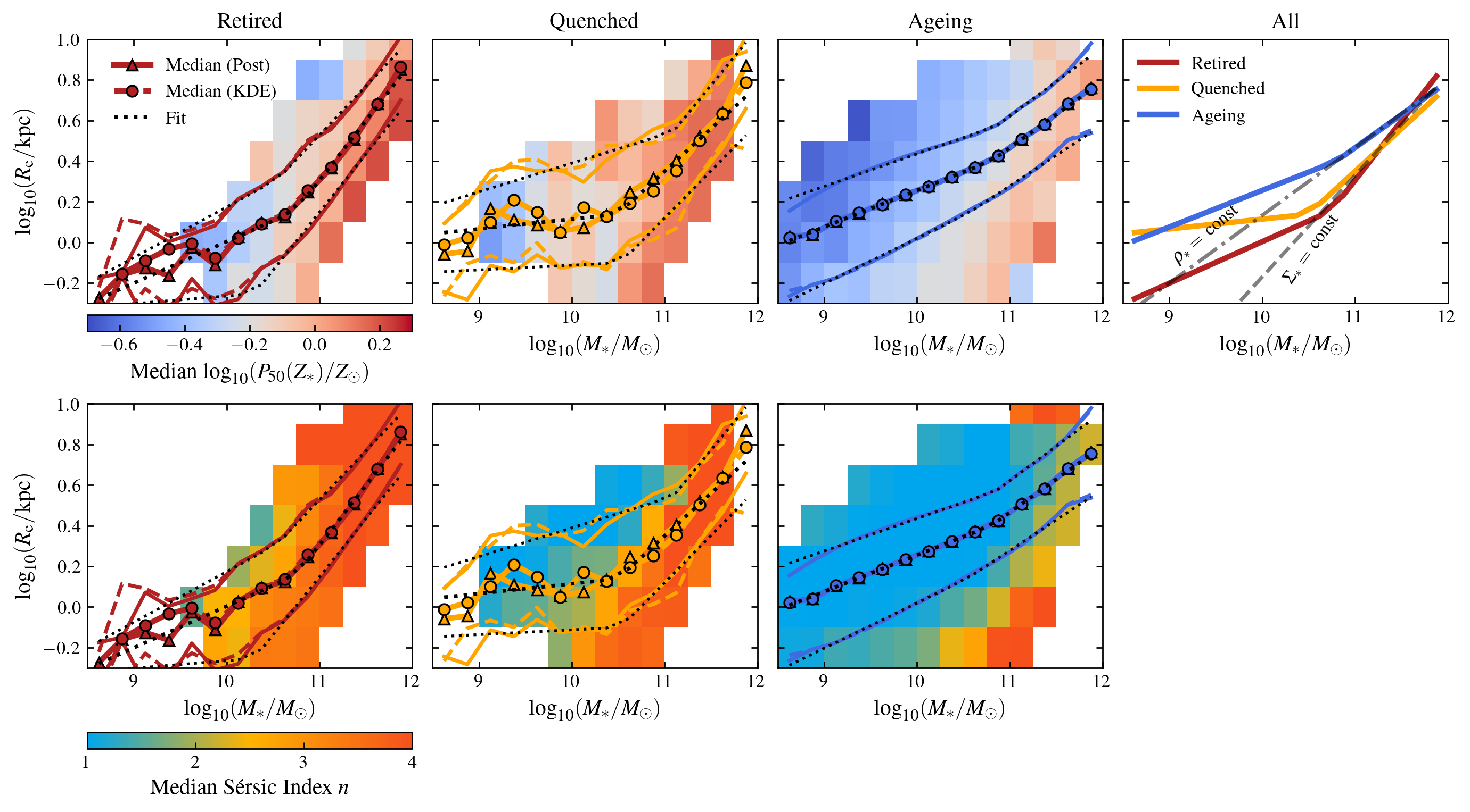
Figure 11: Stellar mass size relation for the full sample of Euclid galaxies. From left to right, panels depict the distribution of Retired, Quenched, Ageing, and the three combined classes across the parameter space. Solid and dashed lines denote the 16th, 50th, and 84th running percentiles computed using the Posterior- and KDE-based classifiers, respectively, adopting the criteria that maximises the $F$-score. The dotted dashed lines denotes the best-fit of Eq. (15) to the percentiles. Top and bottom coloured background maps illustrate the median value per bin of the inferred median stellar metallicity and Sérsic index, respectively, where only bins with more than 10 galaxies have been considered.

Figure 11 shows the distribution of the full sample of Euclid galaxies across the plane defined by their total stellar mass and effective radius, $R_{\rm e}$, used as a proxy for their physical size. The values of $R_{\rm e}$ are derived from Sérsic surface brightness profile fits to VIS Euclid images (see Euclid Collaboration: Cropper et al. 2024; Euclid Collaboration: McCracken et al. 2025, for details on the instrument and data-reduction pipeline). In addition to their excellent spatial resolution, the wide spectral coverage of the $I_{\scriptscriptstyle\rm E}$ band ($5500$–$9000$ Å) provides a robust estimate of galaxy size, being less sensitive to mass-to-light ratio variations compared to optical $ugriz$ photometry. From left to right, the panels present the running 16th, 50th, and 84th percentiles of $R_{\rm e}$ as function of stellar mass, $M_{\ast}$, for Retired, Quenched, and Ageing galaxies, respectively. The background colour maps shown in the top and bottom rows illustrate the median stellar metallicity ($Z_{\ast}$) inferred by BESTA and $I_{\scriptscriptstyle\rm E}$-based Sérsic index ($n$), respectively, restricted to bins with at least 10 galaxies. To quantify the observed trends, we model the percentiles of $R_{\rm e}(M_{\ast})$ using a ‘broken’ power-law model:

$$R_{\rm e}(M_{\ast})=\begin{cases}R_{\rm break}\left(\frac{M_{\ast}}{M_{\rm break}}\right)^{\alpha},&\,M_{\ast}\leq M_{\rm break},\\[4.30554pt] R_{\rm break}\left(\frac{M_{\ast}}{M_{\rm break}}\right)^{\beta},&\,M_{\ast}>M_{\rm break},\\ \end{cases}$$ (15)

where $M_{\rm break}$ represents the characteristic mass where the logarithmic slope transitions between low-mass ($\alpha$) and high-mass ($\beta$) regimes, and $R_{\rm break}$ the predicted effective radius at $M_{\rm break}$. Figure 11 includes black dotted lines showing the best-fit models for each population percentile, with parameters summarised in Table 3. The rightmost panel compares the median relations across the three populations.

Retired galaxies exhibit the steepest correlation between $R_{\rm e}$ and $M_{\ast}$, maintaining consistent slopes ($\beta\simeq 0.5$–$0.6$) across percentiles. They also show systematically the highest values of $n$, aligning with previous results from the literature for early-type or bulge-dominated systems (e.g., Sánchez Almeida 2020). For $M_{\ast}\gtrsim 5\times 10^{10}\leavevmode\nobreak\ {M_{\odot}}$, their distribution roughly follows a line of constant stellar surface density ($\Sigma_{\ast}\simeq 7\times 10^{3}\leavevmode\nobreak\ {M_{\odot}}\,\rm pc^{-2}$). Below this mass, the slope flattens ($\alpha\simeq 0.2$), resembling the distribution of Ageing galaxies. This turnover likely reflects a morphological transition from intermediate-mass red spirals to massive spheroidal systems.

Table 3: Best-fit values of the broken power-law model (Eq. 15) for the mass-size relation presented in Fig. 11.

Percentile	$M_{\rm break}\leavevmode\nobreak\ [{M_{\odot}}]$	$\alpha$	$\beta$	$R_{\rm break}\leavevmode\nobreak\ [\rm kpc]$
Retired
16	$3.5\times 10^{10}$	0.18	0.60	0.7
50	$5.6\times 10^{10}$	0.21	0.59	1.4
84	$3.6\times 10^{10}$	0.25	0.48	2.1
Quenched
16	$3.3\times 10^{10}$	0.02	0.46	0.8
50	$3.2\times 10^{10}$	0.05	0.43	1.4
84	$2.4\times 10^{10}$	0.09	0.29	2.5
Ageing
16	$3.2\times 10^{10}$	0.23	0.28	1.3
50	$6.4\times 10^{10}$	0.18	0.33	2.5
84	$7.7\times 10^{10}$	0.16	0.35	3.8

The mass-size relation for Ageing galaxies is flatter than that of Retired galaxies across the whole mass range. Below $(3$–$5)\times 10^{10}\leavevmode\nobreak\ {M_{\odot}}$, the median $R_{\rm e}$ is parallel to, but offset from, the Retired population by a factor of about $1.6$. Their extended size and low $n$ indicates the presence of prominent discs, that allow Ageing galaxies to sustain moderate-to-high levels of star-formation over large spatial (and temporal) scales. Above $(3$–$5)\times 10^{10}\leavevmode\nobreak\ {M_{\odot}}$, the slope steepens to approximately $R_{\rm e}(M_{\ast})\propto M_{\ast}^{1/3}$, implying constant volumetric stellar density ($\rho_{\ast}$) and characteristic time ($\sqrt{R_{\rm e}^{3}/GM_{\ast}}$).

Quenched galaxies occupy an intermediate position between the other populations. Below around $3\times 10^{10}\leavevmode\nobreak\ {M_{\odot}}$, $R_{\rm e}$ shows little dependence on mass ($\alpha=0.04$–$0.013$), with characteristic sizes of $R_{\rm e}\sim 1$–$1.6$ kpc, indicating higher density and compactness (illustrated by the higher values of $n$) than Ageing galaxies. At $3\times 10^{10}\leavevmode\nobreak\ {M_{\odot}}$, the slope steepens ($\beta=0.36$–$0.47$) bridging the trends of Ageing and Retired populations.

Stellar metallicity ($Z_{\ast}$) complements our findings based on the morphology. Retired galaxies show uniformly high $Z_{\ast}$, aligning with their compact morphology and dense stellar populations, tracing lines of constant $\Sigma_{\ast}$. Ageing galaxies span a wide metallicity range. They are more chemically primitive at lower masses, but we observe a tighter correlation between $Z_{\ast}$ and $\Sigma_{\ast}$ than with $M_{\ast}$. Quenched galaxies exhibit once again an intermediate behaviour, now in terms of chemical enrichment.

In CC23a and CC23b, galaxy quenching was identified as a ubiquitous yet rare process, predominantly affecting low-mass systems in relatively dense environments. Furthermore, CC23a highlighted that present-day Quenched galaxies often exhibit evidence of preceding ‘starburst’ episodes before the cessation of star formation. Combined with their more compact morphologies and richer chemical compositions compared to Ageing galaxies, these findings point to environmental quenching mechanisms (e.g., Wetzel et al. 2013), such as ram-pressure stripping, as the dominant mechanism for shutting down star-formation in the local Universe. The results of this work are consistent with these conclusions, further strengthening the observed links between morphological and chemical properties across the Retired, Quenched, and Ageing galaxy populations.

6 Summary and conclusions

In this study, we have analysed the star-formation histories (SFHs) of a sample of galaxies from Euclid Q1 (Euclid Collaboration: Aussel et al. 2025) spanning the redshift range $0<z<0.8$. Building upon previous work by Corcho-Caballero et al. (2023b, a), we developed a probabilistic classification framework based on the inferred SFH, leveraging two estimates of the average specific star-formation rate (${\rm sSFR}_{\tau}$) measured over distinct timescales ($\tau=\{10^{8},\ 10^{9}\}$ yr). This framework classifies galaxies into three evolutionary classes: Ageing (undergoing secular evolution), Quenched (recently halted star-formation due to a quenching episode), and Retired (dominated by old stellar populations with minimal star-formation).

To test the limits of our classification scheme, we also generated synthetic observations of galaxies from the IllustrisTNG simulation at multiple redshifts. The SFHs were inferred by fitting optical-to-near-infrared photometry across $ugrizY_{\scriptscriptstyle\rm E}J_{\scriptscriptstyle\rm E}H_{\scriptscriptstyle\rm E}$ bands using a Bayesian approach that captures the full posterior probability distribution (Sect. 3.2).

We introduced two classification methods

• Probabilistic Classification: this estimates the likelihood of a galaxy belonging to each class by integrating the posterior probability distribution, in terms of ${\rm sSFR}_{8}$ and ${\rm sSFR}_{9}$, over the regions that delimit each class domain (Sect. 3.1).

• Model-Driven Classification: leveraging IllustrisTNG, this approach optimises sample purity and completeness for each class by exploring the parameter space including additional information from the posterior distribution (Sect. 4.4).

Applying these methods to the Euclid galaxy sample, we estimated the fractions of Ageing, Quenched, and Retired galaxies at low redshift to be approximately 68–72, 8–17, and 14–19%, respectively. These findings align with the results of Corcho-Caballero et al. (2023b), which were based on spectroscopic data, suggesting that photometric classifications can achieve similar reliability.

We studied the fraction of Ageing, Quenched, and Retired galaxies as function of stellar mass. Our results suggest that, at the low mass-end, the number of Quenched galaxies and Retired systems is approximately the same. Conversely, the fraction of Retired galaxies, a smooth increasing function with stellar mass, exceeds the fraction of Quenched systems by a significant factor at masses $\gtrsim 3\times 10^{10}\,{M_{\odot}}$.

We then explored the evolution of the fraction of each class as function of redshift in different stellar mass bins. As expected, the fraction of Ageing galaxies increases with increasing redshift, whereas the fraction of Retired objects presents a strong dependence on stellar mass and redshift: more massive systems become retired earlier as compared to their low-mass counterparts, in line with the ‘downsizing’ picture (Cowie et al. 1996) and the results reported in Euclid Collaboration: Enia et al. (2025). In contrast, the fraction of Quenched galaxies shows mild trends with mass or redshift, and ranges between 5% to 15%. Our results show tentative evidence in favour of an scenario where more massive galaxies usually undergo quenching episodes at earlier times with respect to their low-mass counterparts.

We analysed the differences, in terms of the mass-size-metallicity relation, between Ageing, Quenched, and Retired Euclid galaxies. Ageing galaxies are consistent with a population of late-type galaxies typically dominated by disc morphologies and low stellar metallicities. Retired objects follow a tight sequence in terms of stellar mass and effective radius that matches with that of early-type objects. Above $M_{\ast}\simeq 3\times 10^{10}\leavevmode\nobreak\ {M_{\odot}}$, they arrange along a sequence consistent with constant stellar mass surface density ($\Sigma_{\ast}\simeq 7\times 10^{3}\leavevmode\nobreak\ {M_{\odot}}\,\rm pc^{-2}$). Finally, Quenched galaxies appear as an intermediate population, composed of relatively compact and more chemically evolved systems compared to their Ageing counterparts at a given stellar mass. These characterisation of Ageing, Quenched, and Retired galaxies is in excellent agreement with previous results from Corcho-Caballero et al. (2023a).

These results provide promising directions for understanding the physical mechanisms driving quenching in galaxies. Nonetheless, the heterogeneous sample used in this work might suffer from selection effects and more careful selections are needed to extract more robust conclusions. Fortunately, our study represents a very small region of the sky ($\approx 63$ deg²), compared to expected area surveyed by the Euclid mission (about $14\,000$ deg²). The combination of Euclid photometric data with either Euclid grism spectra and/or ancillary information will enable a far more comprehensive analysis, underscoring Euclid’s transformative potential in unravelling galaxy evolution on cosmological scales.

Appendix A Sample completeness and volume corrections

Table 4: Adopted apparent magnitude flux limit per survey and photometric band.

Band	DESI EDR	2dFGRS	3D-HST	OzDES	PRIMUS	VVDS
$u$	22.48	–	–	–	–	–
$g$	22.19	19.50	23.41	23.36	23.50	23.43
$r$	21.65	18.76	22.39	22.00	23.43	22.54
$i$	21.37	18.42	22.06	21.60	22.06	22.13
$z$	21.46	18.28	21.83	21.40	21.89	21.95
No. sources	9697	845	116	5471	9040	303

This appendix details the methodology used to assess the completeness of our sample and apply volume corrections to account for selection effects. Our approach follows the procedure outlined in Favole et al. (2024).

For each spectroscopic survey contributing to our sample, we estimate the maximum distance at which a galaxy would be detected by considering both a filter-dependent flux limit and the imposed signal-to-noise ratio (S/N) threshold.

To determine the maximum apparent magnitude, $m_{\rm lim}$, for each photometric band in each survey, we compute the 95th percentile of the apparent magnitude in redshift bins. The final $m_{\rm lim}$ is obtained as the median of these percentiles. Table 4 summarises the magnitude limits for each survey.

Galaxies with apparent magnitudes fainter than these limits are discarded. The maximum distance at which a source would still be detected in each band is then given by the maximum distance modulus $\mu(z_{\lim})$, at which a source would be detected on each band as

$$\mu(z_{\lim})=m_{\rm lim}-M-K(z_{\lim}),$$ (16)

where $M$ is the absolute magnitude and $K(z_{\lim})$ is the K-correction at the maximum redshift. The values of $K(z)$ for each source are estimated from the photometric properties of the stellar populations inferred using BESTA (see Sect. 3.2).

We also account for the selection based on S/N by computing the minimum detectable flux for a given noise level

$$f_{\nu,\,\rm lim}={\rm(S/N)_{min}}\,\sigma(f_{\nu,\,\rm obs}),$$ (17)

which translates into a limiting apparent magnitude

$$m_{\lim}=-2.5\log_{10}\left({\rm(S/N)_{lim}}\right)-2.5\log_{10}\left(\sigma\right).$$ (18)

By combining this with Eq. (16), we estimate a second maximum detection distance.

For each galaxy in our sample, we compute two maximum redshifts for each available photometric band, with the final limiting redshift, $z_{\rm max}$, taken as the minimum value across all bands. To estimate the statistical contribution of galaxies in a given redshift bin $(z_{\rm low},z_{\rm up})$, we use the $1/V_{\rm max}$ formalism (Schmidt 1968)

$$V_{\rm max}=\frac{A}{3}\left(d_{\rm L}[{\rm min}(z_{\rm max},z_{\rm up})]^{3}-d_{\rm L}[z_{\rm low}]^{3}\right),$$ (19)

where $A$ is the survey area in steradians and $d_{\rm L}(z)$ is the luminosity distance.

Since our primary interest lies in the relative contributions of different galaxy populations rather than their absolute number densities, we normalise the survey areas relative to the stellar mass function from Baldry et al. (2012). The resulting stellar mass functions in various redshift bins, derived from individual surveys (coloured lines) and the combined data set (black dashed lines), are shown in Fig. 12.

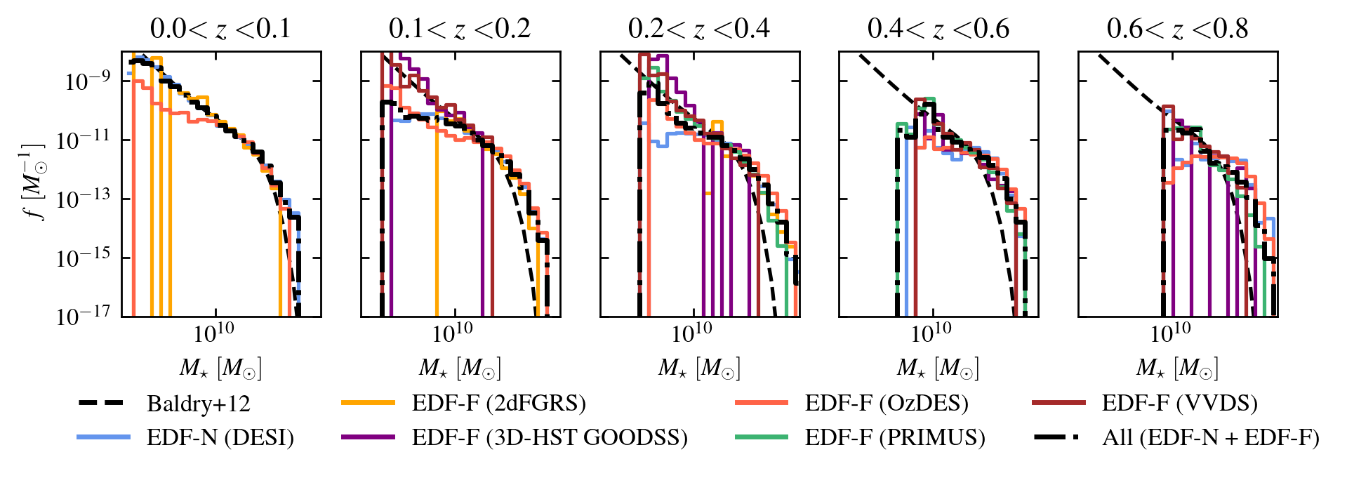
Figure 12: Stellar mass function in different redshift bins. To account for the different effective areas of the surveys, the distributions are normalised between the mass limits of $3\times 10^{10}\leavevmode\nobreak\ {M_{\odot}}$, and $10^{12}\leavevmode\nobreak\ {M_{\odot}}$. Dashed lines denote the double-Schechter fit (restricted to $z\leq 0.06$) from Baldry et al. (2012). Coloured lines denote the resulting mass function from the different surveys that compose the sample. Black dashed-dotted illustrate the resulting mass function of the total sample.

Although the $V_{\rm max}$ correction accounts for selection effects, it remains effective only if a fraction of the missing galaxy population is still detectable. Figure 13 illustrates the completeness limits for Quenched and Retired galaxies as a function of redshift and stellar mass.

These limits are estimated using the 5th percentile and the minimum value of ${\rm sSFR}_{8}$ and ${\rm sSFR}_{9}$ in each redshiftstellar mass bin. The bottom panel of Figure 13 provides an absolute detection limit for each galaxy class, indicating the regime where volume corrections are still valid. The top panel presents a more conservative threshold.

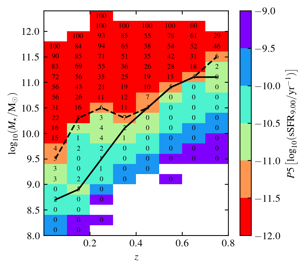
Figure 13: Completeness of Retired galaxies in terms of $z$, and $M_{\ast}$. The coloured map illustrates the 5th percentile of ${\rm sSFR}_{9}$ on each $z$–$M_{\ast}$ bin. Each bin includes the (uncorrected) fraction of Retired galaxies with respect to the total, based on the classification that maximises the $F$-score. The dashed and solid lines denote the mass completeness limit above which Retired galaxies are detected. Each line tracks the lower envelope that satisfies ${\rm sSFR}_{9}<10^{-11}\,\rm yr^{-1}$ and ${\rm sSFR}_{8}<3\times 10^{-11}\,\rm yr^{-1}$, based on the 5th and 1st percentiles, respectively.

Appendix B SFH inference performance as function of redshift

Figure 14: Same as Fig. 2 but restricted to the estimates at $z=0$.

In this appendix, we present the results obtained from fitting the IllustrisTNG $ugrizY_{\scriptscriptstyle\rm E}J_{\scriptscriptstyle\rm E}H_{\scriptscriptstyle\rm E}$ photometry with BESTA as function of their observed redshift. Figures 14, 15, and 16 show the true input values of ${\rm sSFR}_{\tau}$ versus the median value recovered by BESTA for the realisations at $z=0.0,\,0.3$, and $0.6$, respectively, complementing Fig. 2.

The effect of redshifting the SED of our sample of galaxies has a significant impact on the performance of the recovery of the values of ${\rm sSFR}_{\tau}$. From $z=0$ to $z=0.6$, we find a progressive improvement in the performance of the fits illustrated by the reduction of the scatter along the one-to-one line. The number of catastrophic outliers also seems to decrease, especially for $\tau\geq 10^{9}\,\rm yr$. On the other hand, the fraction of sources whose input value of ${\rm sSFR}_{\tau}$ is within the 68 and 90% credible intervals decreases in most of the cases with respect to the realisation at $z=0$, implying that the estimate of the posterior probability distribution might be too sharp and the uncertainties are underestimated.

Figure 15: Same as Fig. 2 but restricted to the estimates at $z=0.3$.

Figure 16: Same as Fig. 2 but restricted to the estimates at $z=0.6$.