Euclid Quick Data Release (Q1)

The extent to which the environment affects galaxy evolution has been under scrutiny by researchers for decades. With the first data from Euclid, we can begin to systematically study a wide range of environments and their effects as a function of redshift, using $63\,\text{deg}^{2}$ of space-based data. In this paper, we present results from the Euclid Quick Data Release, where we measure the passive-density and morphology-density relations in the redshift range $z=0.25$–$1$. We determine if a galaxy is passive using the specific star-formation rate, and we classify the morphologies of galaxies using the Sérsic index $n$ and the $u-r$ colours. We measure the local environmental density of each galaxy using the $N\text{th}$-nearest neighbour method. This gives a measure of the local density in units of $\text{gal}\ \text{Mpc}^{-2}$. We find that at fixed stellar mass, the quenched fraction (galaxies that have ceased star formation) increases with increasing local environmental density up to $z=0.75$. This result is indicative of the separability of the effects from the stellar mass and the environment, at least at $z<0.75$. At $z>0.75$, we observe only weak environmental effects, with most galaxies with $M_{\ast}\gtrsim 10^{11}\ M_{\odot}$ being quenched independently of environment. Up to $z=0.75$, the early-type galaxy fraction increases with increasing density at fixed stellar mass, meaning the environment also transforms the morphology of the galaxy independently of stellar mass, up to $M_{\ast}\lesssim 10^{10.8}\ M_{\odot}$. For $M_{\ast}\gtrsim 10^{10.8}\ M_{\odot}$, almost all galaxies are early-types, with minimal impact from the environment. At $z>0.75$, the morphology depends mostly on stellar mass, with only low-mass galaxies being affected by the environment. Given that the morphology classifications use $u-r$ colours, these are correlated to the star-formation rate, and as such our morphology results should be taken with caution, yet future morphology classifications should help verify these results. To summarise, we successfully identify the passive-density and morphology-density relations at $z<0.75$, but at $z>0.75$ the relations are less strong, only affecting certain mass bins. At $z>0.75$, the uncertainties on both photometric redshift and stellar masses are large, and thus future Euclid data releases are key to confirm these trends.

1 Introduction

It is clear that the environment plays a significant role in the evolution of galaxies at low redshift. The passive-density relation shows that galaxies in higher density environments such as groups or clusters are more likely to be quenched than galaxies in the field of the same stellar mass (Peng et al. 2010; Vulcani et al. 2010; Wetzel et al. 2012; Paccagnella et al. 2016; Darvish et al. 2017; Cleland & McGee 2021; Corcho-Caballero et al. 2023). Moreover, this effect is more prominent in low-stellar mass satellite galaxies $(M_{\ast}\lesssim 10^{10}\,M_{\odot})$, while at higher mass, the quenched fractions of satellite galaxies and central galaxies evolve similarly (Cleland & McGee 2021; Corcho-Caballero et al. 2023), meaning the environment is not preferentially affecting one class of galaxy over another. This phenomenon of quenching at high masses has been described as ‘mass-quenching’ (Peng et al. 2010), and loosely encompasses the quenching mechanisms that occur irrespective of the environment. These quenching mechanisms are also referred to as ‘internal quenching mechanisms’, to distinguish them from ‘external quenching mechanisms’ by the environment. Furthermore, the morphology-density relation is well-studied at low-$z$: galaxies in high-density environments tend to have more spheroidal morphologies, whereas galaxies in the field are more discy (Dressler 1980; Kauffmann et al. 2003; Postman et al. 2005). It should be noted that, while the star-formation rate and morphology of a galaxy are related, they are not the same thing, and the processes that affect them operate in different ways. In other words, many galaxies are passive and early-type, or blue and late-type, but there exist populations of red spirals and blue ellipticals at low redshift (Masters et al. 2010; Rowlands et al. 2012; Tojeiro et al. 2013; McIntosh et al. 2014; George & Zingade 2015; George 2017), as well as at high redshift (Mei et al. 2006, 2015; Fudamoto et al. 2022; Mei et al. 2023). The observed differences between these populations are indicative of distinct formation pathways, at low and high redshift. Thus, it is important to disentangle how the star formation and the morphology of galaxies are evolving separately.

Table 1: Sample selection constraints and limits. The name of the column in the Euclid data products is listed, along with the criterion applied. The column ‘number in sample’ is the number of galaxies at $0.25<z<1$ after that one criterion has been applied. The final sample is the result of applying all the criteria. Note that the $H_{\scriptscriptstyle\rm E}$ flux has been converted to a magnitude using the zeropoint of 23.9.

Euclid data products column name	Criterion	Number in sample
PHZ_MEDIAN	$0.25<z<1$	$1\,285\,305$
mag(FLUX_H_TEMPLFIT)	$<24$	$1\,276\,629$
DET_QUALITY_FLAG	$<4$	$1\,224\,267$
PHZ_FLAGS	$<11$	$1\,209\,143$
PHZ_PP_MEDIAN_SFHAGE	$>0.15$ Gyr	$1\,107\,461$
$|\,\texttt{PHZ\_MEDIAN}-\texttt{PHZ\_PP\_MEDIAN\_REDSHIFT}\,|$	$<0.1\times\texttt{PHZ\_MEDIAN}$	$717\,453$
$|\,\texttt{PHZ\_PP\_MEDIAN\_SFR}-\texttt{PHZ\_PP\_MODE\_SFR}\,|$	$<0.5$	$1\,077\,691$
Final sample		$538\,094$

These results in the local Universe paint a picture where high-density environments have a transformative effect on a galaxy’s star-formation processes and its morphology. These environmental effects include ‘starvation’, a process which prevents the accretion of cool fresh gas onto the galaxy (Larson, Tinsley, & Caldwell 1980; Balogh, Navarro, & Morris 2000), and ‘ram-pressure stripping’, whereby the gas reservoir of the galaxy is rapidly removed after infall to the cluster (Gunn & Gott 1972). Moreover, the structure of the galaxy may be affected by ‘harassment’, where increased tidal forces between the galaxy and the cluster, and high-speed encounters with other galaxies, can disrupt the stellar disc (Moore et al. 1996), and by increased rates of mergers in certain environments, which transform the morphology of the galaxy while also accelerating star formation, leading to eventual quenching (Toomre & Toomre 1972).

This picture is less clear at $z>1$. There is much work ongoing in search of massive passive galaxies at high redshifts (particularly at $z>2$; Straatman et al. 2016; Merlin et al. 2018, 2019; Carnall et al. 2023, 2024), however, observing these objects is still a challenge. Quantifying the environments in which they reside is even more difficult. The extent to which the environment affects galaxy properties, and the epoch at which this begins, is under much scrutiny. Notably, the high-density environment looks very different at $z=1$–$2$ compared to that at low $z$. There have been many studies on various observed ‘proto-clusters’ (Chiang, Overzier, & Gebhardt 2013; Overzier 2016; Chiang et al. 2017; Lovell et al. 2018), which form the candidate progenitors of galaxy clusters at $z=0$. In the Spiderweb protocluster at $z=2.2$, there is no strong evidence of an environmental effect on the star formation or morphology of the galaxies (Pérez-Mart´ınez et al. 2023). However, in a different Spiderweb study, it was found that four out of five massive star-forming galaxies may host active galactic nuclei (AGN), which may eventually suppress star formation and quench the galaxy (Shimakawa et al. 2018). In a study of clusters and proto-clusters at $1.3<z<2.8$, there is already evidence of the passive-density relation at $z\sim 2$ (Mei et al. 2023). By $z\simeq 1.6$, cluster galaxies show strong radial colour gradients compared to field galaxies (Cramer et al. 2024), implying the onset of environmental quenching between $z\approx$ and $z\approx 1$ (Edward et al. 2024). Equally, the redshift at which the morphology-density relation first appears is uncertain. In $z\simeq 1$ clusters, there is a clear increase in the fraction of early-type galaxies (ETGs) at higher local densities ($>1000\ \text{gal}\,\text{Mpc}^{-2}$, Postman et al. 2005). Further, as demonstrated by Mei et al. (2023), the morphology-density relation is found to exist at $z\simeq 2$, however more statistics are needed to confirm if the relation is present at $z>2$.

These results suggest the importance of the cluster and proto-cluster environment in building up the star formation of galaxies, and then rapidly quenching them (Elbaz et al. 2007; Wang et al. 2016). However, identifying large samples of high-density environments over a large redshift range is a challenge. The Euclid mission (Euclid Collaboration: Mellier et al. 2024) is well-suited to overcome these challenges. The Euclid Wide Survey (Euclid Collaboration: Scaramella et al. 2022) aims to observe up to $14\,000\ \text{deg}^{2}$, providing high-resolution data on billions of galaxies. The size of the Euclid footprint, and the addition of external ground-based data (Euclid Collaboration: Romelli et al. 2025; Rhodes et al. 2017) will allow for local galaxy density measurements in a wide range of environments, at this key epoch of galaxy evolution, at $z\approx 1$.

In this paper, we use data from the Euclid Quick Release Q1 (2025) to investigate the significance of the environment in quenching galaxies and transforming their morphology, as a function of redshift. We calculate the local environmental density for each galaxy, and use that to measure the passive-density and morphology-density relations as functions of redshift. This paper is organised as follows: Sect. 2 describes the data used, and how we derive the measurements of local environmental density; Sect. 3 explains our results for the passive-density relation and the morphology-density relation; finally, Sect. 4 discusses these results in the context of other studies and summarises our results. For cosmological calculations, we use the Planck cosmological parameters, Planck Collaboration et al. (2016): $\Omega_{\text{m}}=0.313$, $\Omega_{\Lambda}=0.687$, $\Omega_{\text{b}}=0.048$, $H_{0}=67.31\ \text{km s}^{-1}\ \text{Mpc}^{-1}$, and $n_{\text{s}}=0.966$.

2 Data

2.1 Euclid data

The Euclid Quick Release Q1 (2025) consists of observations of three fields, Euclid Deep Field North (EDF-N), Euclid Deep Field South (EDF-S), and Euclid Deep Field Fornax (EDF-F), consisting of $22.9\,\deg^{2}$, $28.1\,\deg^{2}$, and $12.1\,\deg^{2}$, respectively (Euclid Collaboration: Aussel et al. 2025). This release consists of data products from the OU-MER pipeline (Euclid Collaboration: Romelli et al. 2025), which includes galaxy coordinates, photometric data from the VIS (Euclid Collaboration: McCracken et al. 2025) and NISP (Euclid Collaboration: Polenta et al. 2025) instruments, external data, and also morphology information, such as the Sérsic index from SourceXtractor++ (Bertin et al. 2020; Kümmel et al. 2022), and other morphological parameters acquired by machine learning (Euclid Collaboration: Romelli et al. 2025). The visible filter, $I_{\scriptscriptstyle\rm E}$ reaches a $5\,\sigma$ point-source sensitivity of 24.5 mag (Euclid Collaboration: Cropper et al. 2024), and the NIR filters, $Y_{\scriptscriptstyle\rm E}$, $J_{\scriptscriptstyle\rm E}$, and $H_{\scriptscriptstyle\rm E}$ each reach 24 mag (Euclid Collaboration: Jahnke et al. 2024). For a detailed overview of the Euclid mission, we refer the reader to Euclid Collaboration: Mellier et al. (2024).

Photometric redshifts and galaxy physical properties are produced by OU-PHZ (Euclid Collaboration: Tucci et al. 2025), using two different methods. The Phosphoros model provides Bayesian posterior distributions of photometric redshifts, and these are the redshifts we use in this work. Uncertainties on these redshifts are taken as the $68\,\%$ upper and lower limits on these distributions. The other model, Nearest-Neighbour Photometric Redshifts (NNPZ), returns galaxy physical properties, including stellar masses, star-formation rates (SFRs) based on a Kroupa IMF (Kroupa 2001), and galaxy ages, using the 30 nearest neighbours from a calibration sample in the multi-dimensional phase-space (Euclid Collaboration: Tucci et al. 2025). A delayed exponential star-formation history model is used to generate the model spectral energy distributions, and two dust extinction laws are used, Calzetti et al. (2000) and Prevot et al. (1984); full details can be found in Euclid Collaboration: Tucci et al. (2025). For the stellar masses, star-formation rates, and galaxy ages, we use the medians of the posterior distributions provided by NNPZ. We then measure the specific star-formation rate (sSFR) by dividing the SFR by the stellar mass, i.e., $\text{sSFR}=\left(\text{SFR}/M_{\ast}\right)$.

From the total sample, we remove sources that are saturated, masked by stars, masked by extended objects, or are too faint for reliable photometric measurements. We impose a magnitude limit of $H_{\scriptscriptstyle\rm E}$ $<24$. Additionally, we consider only a robust sample of galaxies for which the photometric redshift estimates from Phosphoros and NNPZ agree within $10\%$. For this we use the medians of the redshift distributions from Phosphoros (PHZ_MEDIAN) and NNPZ (PHZ_PP_MEDIAN_REDSHIFT), such that $|\,\texttt{PHZ\_MEDIAN}-\texttt{PHZ\_PP\_MEDIAN\_REDSHIFT}\,|<0.1\times\texttt{PHZ\_MEDIAN}$. Similarly, we require robustly estimated star-formation rates, such that the first mode and the median of the posterior distribution agree within $0.5$. Finally, we remove galaxies with unphysically high sSFRs (an atypical peak at $10^{-8}\ \text{yr}^{-1}$) by imposing a lower limit in age of $0.15\,\text{Gyr}$ (see Euclid Collaboration: Enia et al. 2025; Euclid Collaboration: Tucci et al. 2025, for details). This cut on the age removes $15\,282$ galaxies from the final sample. These quality cuts are listed in Table 1. Our final sample contains $538\,094$ galaxies at $0.25<z<1$. It is clear that the cut involving the two different redshifts removes a large number of galaxies from the final sample. This is partly explained by the choice of tolerance, of $10\%$, which is quite low at low $z$. Furthermore, the redshift estimation is less reliable at low redshift, particularly in NNPZ, leading to a large number of mismatches. These mismatches are removed with this cut. However, these cuts introduce some possible incompleteness, particularly at $z\approx 1$. We caution that these results are not yet fully robust, however work is ongoing to correct for this incompleteness.

2.2 Density measurements

The local environmental density is calculated for each galaxy using the $N$th-nearest neighbour method (Postman et al. 2005; Mei et al. 2023). For this calculation and subsequent results, we include only galaxies with $M_{\ast}>10^{9.5}\ M_{\odot}$, which we calculated as the 85% stellar mass completeness limit for passive galaxies at $z=1$, following Pozzetti et al. (2010). The density is calculated as $\Sigma_{N}={N}\,/\left({\pi\,D^{2}_{N}}\right)$, where $N$ is the number of galaxy neighbours and $D_{N}$ is defined as the on-sky distance to the $N$th-nearest neighbour. Results are stable in the range $N=5$–$10$, and we use $N=7$ to be consistent with previous galaxy projected surface density estimates (Postman et al. 2005; Mei et al. 2023).

For every galaxy in the final sample, we calculate the comoving distance to the $7$th-nearest neighbour, within a redshift slice $\Delta z$ centred on the galaxy. This redshift slice corresponds to 3 times the median uncertainty (the difference between the redshift and the average of the $68\,\%$ upper and lower limits) on the redshift in each photometric redshift bin, i.e., $3\ \sigma$ (listed in Table 2). Note that in the highest redshift bin, $z=0.75$–$1$, the density calculation includes galaxies at higher redshifts within the redshift slice. This ensures we do not miss any nearby galaxies that are outside the redshift bin. We note that the large uncertainties on the photometric redshifts result in a large range of redshift to search for overdensities, which may ultimately smooth out any environmental effects at high $z$. We divide the number of galaxies (in this case, this is $7$) by the on-sky distance to the $7{\text{th}}$-nearest neighbour in the redshift slice to obtain the surface density of galaxies, $\Sigma_{7}$. This corresponds to the number of galaxies within an on-sky area with radius $1\ \text{Mpc}$. We calculate uncertainties on $\Sigma_{7}$ by propagating the uncertainties on the photo-$z$s in the cosmological distance measurement, and the Poissonian uncertainties in counting the number of nearby galaxy neighbours, i.e., $\sqrt{7}$. Hereafter, we refer to $\Sigma_{7}$ as density.

Table 2: Median uncertainty on the redshift for each redshift bin.

Redshift bin $(z)$	Median uncertainty $(\text{d}z)$
$0.25$–$0.50$	$0.045$
$0.50$–$0.75$	$0.045$
$0.75$–$1.00$	$0.070$

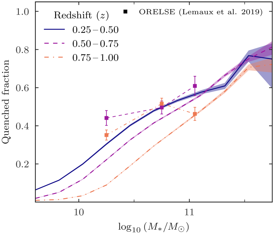
Figure 1: Fraction of galaxies classes as quenched as a function of stellar mass, binned by redshift. Shaded regions show $68\,\%$ confidence intervals. Only bins where the total number of galaxies is greater than 10 are plotted. ORELSE quenched fractions (Lemaux et al. 2019) are plotted in coloured squares. Their fractions are higher on average, likely because they purposely probe areas with larger galaxy densities than the Q1 fields.

3 Results

3.1 Quenched fraction

First, we consider quenched galaxies, which are galaxies in which star formation was suppressed. We determine if a galaxy is quenched following the criterion in Franx et al. (2008), that is, if $\text{sSFR}<0.3\,t_{\text{H},z}^{-1}$, where $t_{\text{H},z}$ is the Hubble time at a given redshift, which gives a timescale for the expansion of the Universe at that redshift. This means that the threshold in sSFR for a galaxy to be considered quenched changes with redshift: at $z=0$ this threshold is $-10.68$ and at $z=1$ it is $-10.43$. This is due to the fact that the average galaxy sSFR on the main sequence also increases with redshift at a given mass (Speagle et al. 2014).

We find that the number of passive galaxies in the data drops significantly at $z>1$, likely due to the depth of the optical surveys in the Q1 area that causes a lack of high quality photometric redshifts at high $z$. Thus, for the current work, we limit our analysis to $z\leq 1$. In Fig. 1, we plot the quenched fraction as a function of stellar mass, binned by redshift.

We compare our results to the quenched fractions from the Observations of Redshift Evolution in Large-Scale Environments (ORELSE, Lemaux et al. 2019) survey. This survey studied quenched fractions in a large range of environments, in the redshift range $0.55<z<1.4$. Quenched galaxies are selected using NUV, $r$ and $J$ colours. Their passive selection corresponds to galaxies with $\text{sSFR}<10^{-11}\,\text{yr}^{-1}$, which is a slightly more conservative cut than ours. In Fig. 1, we plot the ORELSE quenched fractions in the mass and redshift bins provided in their Table 3. We see a steady increase in the quenched fraction from $10^{10}\ M_{\odot}$ to $>10^{11.5}\ M_{\odot}$, reaching $60$–$80\,\%$ at the high-mass end.

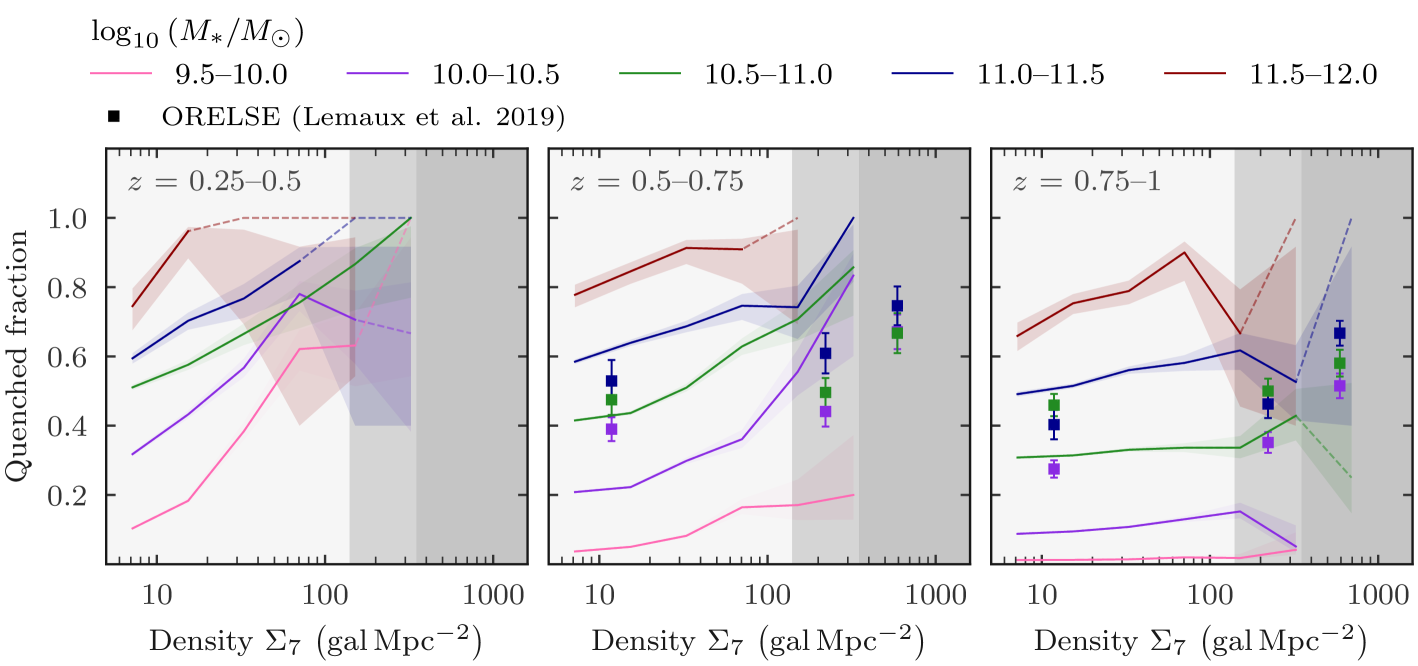
Figure 2: Fraction of galaxies classed as quenched as a function of galaxy density, binned by stellar mass and redshift. The stellar mass bins listed in the legend are in units of $\operatorname{log_{10}}(M_{\ast}/M_{\odot})$. The grey shaded regions in the background refer to the three density bins used in Lemaux et al. (2019), see text for details. The colour shaded regions show $68\,\%$ confidence intervals. Dashed lines indicate density bins where the total number of galaxies is less than 5.

There is generally a discrepancy between our quenched fractions and the ORELSE quenched fractions, of at most about $10$–$20\,\%$, although we note the sample size for ORELSE, $5000$ spectroscopically confirmed galaxies, is much smaller than ours. However, even taking error bars into account, our quenched fractions are considerably lower than the ORELSE fractions. This is particularly true at the low mass end. The cause of this discrepancy might be due to the fact that ORELSE targeted high-density environments, which would have higher fractions of passive galaxies. However, we also note that our fractions have not been corrected for the quenched and star-forming galaxies selection functions, since they are not yet available for Q1. Therefore, this result should be confirmed with further Euclid photometry characterization.

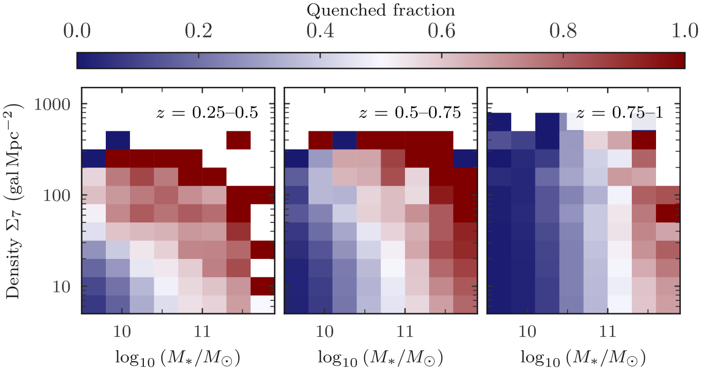
Figure 3: Distribution of the quenched fraction as a function of both stellar mass and galaxy density, in bins of increasing redshift from left to right. The colour-bar indicates the mean quenched fraction in each bin. The separability of the impact of stellar mass and the environment on the quenched fractions is clearly visible up to $z=0.75$, after which the stellar mass dominates the quenching effects.

Qualitatively, the behaviour in Fig. 1 compares well with results described in two other Q1 papers. Euclid Collaboration: Corcho-Caballero et al. (2025) finds the fraction of slowly-quenched galaxies is approximately $60\%$ at $0.6<z<0.8$ at $M_{\ast}>10^{11}\,M_{\odot}$. Similarly, Euclid Collaboration: Enia et al. (2025) report a decrease in the fraction of passive galaxies with increasing redshift. We stress these two Q1 papers classify star-forming/quenched galaxies differently to how we do, so it is to be expected that there is slight variance in the fractions of quenched galaxies reported. Here, they report for all galaxies above their $95\%$ completeness limit ($\approx 10^{9}\,M_{\odot}$ at $z\sim 1$), a quenched fraction of $23\%$ at $0.2<z<0.5$, $15\%$ at $0.5<z<0.8$, and $8\%$ at $0.8<z<1.5$. When computing the quenched fraction for all galaxies in our sample with $10^{9.5}<M_{\ast}\,/\,M_{\odot}<10^{12}$, we find fractions of $23\%$ at $0.25<z<0.5$, $21\%$ at $0.5<z<0.8$, and $12\%$ at $0.8<z<1$. Note that we do not have exactly the same redshift bins. The relative increase of the quenched fraction in our sample compared to theirs in the last redshift bin can be explained by the fact that their bin will have even more star-forming galaxies at $z>1$, diluting their quenched fraction at that redshift. We find our results qualitatively match these two papers well despite using different methods to classify quenched galaxies. However, we cannot exclude biases in the galaxy photometry and from the large uncertainties in photometric redshift that could potentially impact these analyses.

We plot the quenched fraction as a function of environmental density in Fig. 2. Galaxies are binned by stellar mass and by redshift. Again, we plot the ORELSE quenched fractions. They calculate their density $\operatorname{log_{10}}(1+\delta)$ using a Voronoi Monte-Carlo method (see Lubin et al. 2009; Tomczak et al. 2017). They presented their results in three environmental density bins: low density $\operatorname{log_{10}}(1+\delta)<0.3$, intermediate density $0.3<\operatorname{log_{10}}(1+\delta)<0.7$, and high density $\operatorname{log_{10}}(1+\delta)>0.7$. These density bins may be converted to bins in $\Sigma_{7}$, and the result is $\Sigma_{7}<140\ \text{gal}\ \text{Mpc}^{-2}$, $140<\Sigma_{7}\,/\,\text{gal}\ \text{Mpc}^{-2}<350$, and $\Sigma_{7}>350\ \text{gal}\ \text{Mpc}^{-2}$ for low-, intermediate-, and high-density bins, respectively (Mei et al. 2023). It has been shown by Darvish et al. (2015) that the conversion between the nearest-neighbour method and the Voronoi Monte-Carlo method works well, and at the same depth as this work. The ORELSE density bins are indicated on Fig. 2 by the grey shaded regions. It is clear that the quenched fraction increases with local environmental density at all stellar masses, up to $z=0.75$. At $0.75<z<1$, only galaxies with $M_{\ast}>10^{11}\,M_{\odot}$ exhibit this behaviour. We plot the quenched fractions from the ORELSE survey (Lemaux et al. 2019), in the same stellar mass and redshift bins.

Quantitatively, we find that the the differential change in fraction as a function of density, which corresponds to the overall slope of each coloured line in Fig. 2, indeed decreases with increasing redshift. Here, the slope is an indicator of how strongly the environment affects the quenched fraction, such that a higher slope means a stronger impact. Notably, the slope decreases over the range $z=0.6$ to $z=0.8$, and by $z=1$, the slope is $<0.2$ at all stellar masses, and very close to 0 for $M_{\ast}<10^{11}\,M_{\odot}$. We also find that the overall decrease in the slope (i.e., the change in the impact of the environment with increasing redshift) is larger for low-mass galaxies with $M_{\ast}<10^{10.5}\,M_{\odot}$, whereas the decrease in the slope for high-mass galaxies is shallower.

In order to further verify that the quenching effect does not simply trace the stellar mass, we plot the 2-dimensional distribution of the quenched fraction with respect to the stellar mass and density in Fig. 3. Here, galaxies are binned by stellar mass and local density, and panels from left to right show increasing redshift bins. The colour-bar shows the quenched fraction in each bin, such that redder bins contain a higher number of quenched galaxies compared to bluer bins, which are mostly star forming. The size of the bins on the $x$-axis and $y$-axis are determined by the typical uncertainties in the stellar mass and local density, respectively. In the figure, we see that at fixed stellar mass, the quenched fraction increases with increasing local environmental density, up to $z=0.75$. At $z<0.5$, the effect from the environment is strongest for low-mass galaxies, and gets weaker with increasing stellar mass. At $0.5<z<0.75$ the effect does not change much with stellar mass. This behaviour illustrates how the environment of a galaxy can quench its star formation, at fixed stellar mass, reflective of the result in Peng et al. (2010), which is for the red fraction of SDSS galaxies at $z<0.2$. Although, there are differences between these results. Following the line in Fig. 3 where the quenched fraction is equal to $0.5$, the line shows little to no curve. The line where the red fraction is equal to $0.5$ in Fig. 6 of Peng et al. (2010) is more curved, implying that there is a density threshold (mass threshold) after which quenching can happen at fixed stellar mass (density). On the other hand, our results imply a more continuous change with increasing stellar mass or densit, at least at $0.75$. At $z>0.75$, we observe only weak effects from the environment; most galaxies below $M_{\ast}=10^{11}\ M_{\odot}$ are not quenched, regardless of the environment. At higher masses, there is a weak environmental signal. It is worth noting that in this last redshift range, the uncertainty on both photometric redshift and stellar masses increases, and future reprocessing and recalibration of Euclid data, and increased observations will be beneficial to confirm these trends.

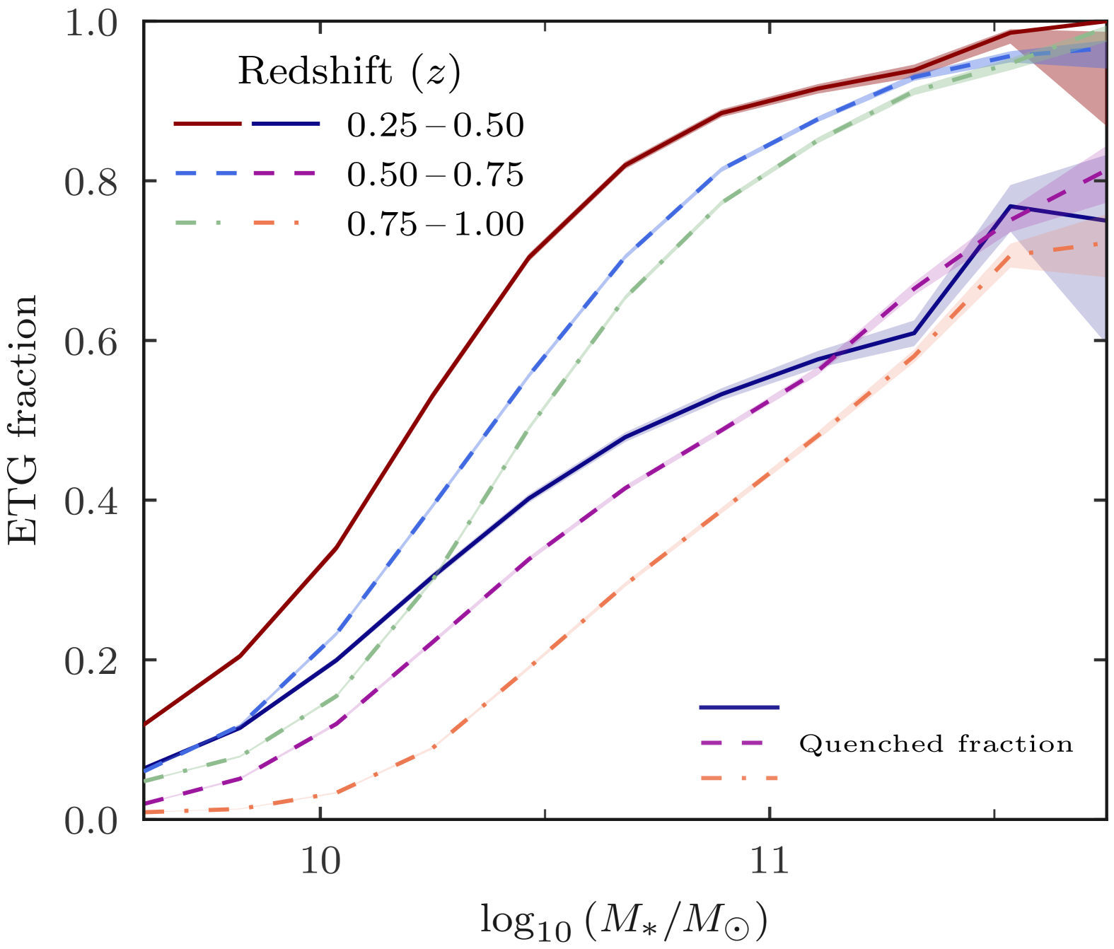
Figure 4: Fractions of galaxies classed as ETGs as a function of stellar mass, binned by redshift. Shaded regions show $68\,\%$ confidence intervals. Only bins where the total number of galaxies is greater than 10 are plotted. The quenched fractions from Fig. 1 are plotted for comparison in the same redshift bins. The ETG fraction increases with stellar mass at all redshifts.

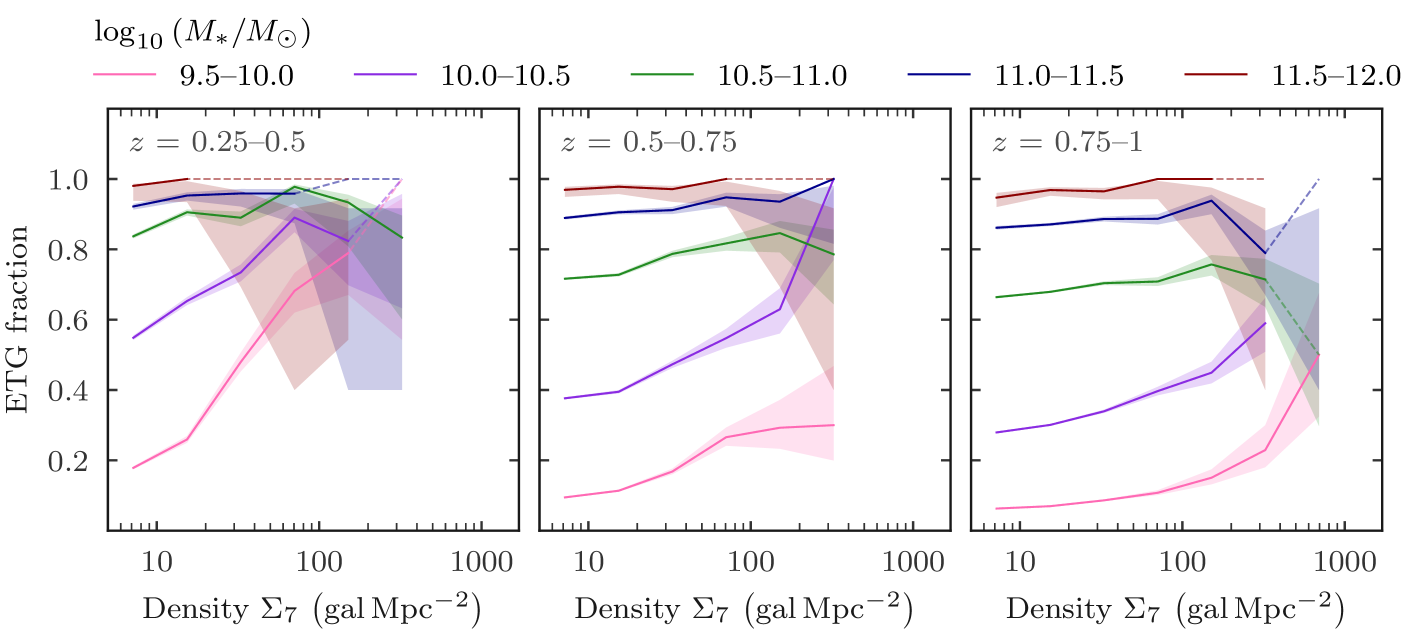
Figure 5: Fraction of galaxies classed as ETGs as a function of galaxy density, binned by stellar mass and redshift. Shaded regions show $68\,\%$ confidence intervals. Dashed lines indicate density bins where the total number of galaxies is less than 5. Up to $z\sim 0.75$, there is a significant increase in the ETG fraction of galaxies from low density environments to high density environments, for low-mass galaxies. However, more massive galaxies are already mostly ETGs. At $z>0.75$, the environment only weakly affects the ETG fraction.

3.2 Morphology

Usually, galaxy morphological classification is based on galaxy specific visual features, such as the presence of a bulge or a disk and their respective predominance in the rest-frame $B$ band (for an example at $z\sim 1$, see Postman et al. 2005). However, for our sample the rest-frame $B$ band corresponds to $i$ and $z$ apparent magnitudes, which are not observed by Euclid. Therefore, we use the morphological classification from Euclid Collaboration: Quilley et al. (2025, hereafter Q25) to identify early-type (ETG) and late-type (LTG) galaxies. This classification is based on the separation of these two galaxy morphological types in the Sérsic index, $n$, vs. the $u-r$ colour plane. We note that, since this classification uses colour, this is not a classification exclusively based on visual features. Our ETG sample will be biased towards red galaxies. This means that while the ETG sample contains a mix of passive and star-forming galaxies, almost every passive galaxy is an ETG ($90\%$). This is an unavoidable degeneracy at this stage, and as such results should be interpreted cautiously. However machine-learning based classifications should be available for Euclid data in the future (Dom´ınguez Sánchez et al. 2022).

ETGs are separated from LTGs by a demarcation line (Eq. 4 in Q25), such that ETGs are located above this line, and LTGs are below it. The equation for this line is in Eq. 1 below:

$$(u-r)_{\text{lim},n}=2.32-1.32\log_{10}(n).$$ (1)

We plot the ETG fraction as a function of stellar mass, in bins of redshift, in Fig. 4. We also plot the quenched fraction from Fig. 1 for comparison. Here, we see a rise in the ETG fraction up to $90\,\%$ in the most massive galaxies. The ETG fraction also increases with decreasing redshift. We do not plot ETG fractions at $z>1$ because, as with the passive galaxies, the Q25 morphological classification is less reliable at these high redshifts.

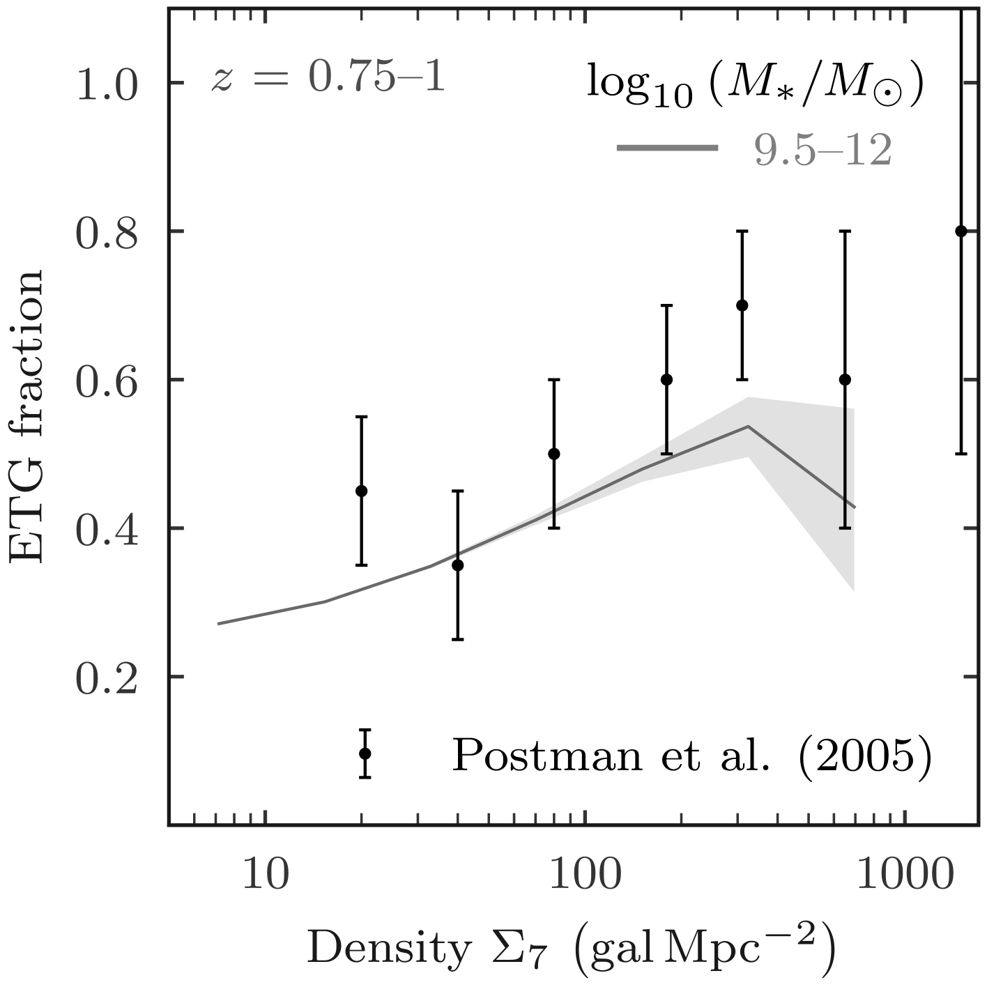
Figure 6: Fraction of ETGs as a function of galaxy density, in the highest redshift bin $0.75<z<1$. The stellar mass range is shown in the top right corner. The ETG fractions from the entire cluster sample of Postman et al. (2005) are plotted in black dots. The two samples are comparable, as they are selected at roughly the same depth, however photometric redshift uncertainties in the Euclid sample are larger, and the morphological classifications are not done in the same way, which may possibly lead to differences in the ETG fractions.

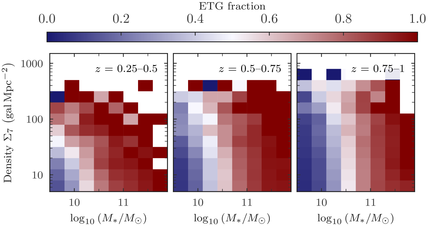
Figure 7: Distribution of the ETG fraction as a function of both stellar mass and galaxy density, in increasing redshift bins from left to right. The colour-bar indicates the mean ETG fraction in each bin. Similar to in Fig. 3, the separability of the stellar mass and environment in producing the ETG fraction is clear up to $z=0.75$. However, it is most evident only up to $M_{\ast}\approx 10^{10.8}\ M_{\odot}$, after which, almost all galaxies are ETGs, regardless of the environment.

Similar to Fig. 2, we plot the ETG fraction as a function of local density in Fig. 5. In the lowest redshift bin, we see a significant increase in the ETG fraction of galaxies with $M_{\ast}<10^{10.5}\ M_{\odot}$ from low density environments to high density environments. More massive galaxies are already mostly ETGs, as seen in Fig. 4. At $0.5<z<0.75$, the morphology-density relation is still present but less prominent. At $z>0.75$ the effect of the environment is weaker. There is slight evidence of an environmental effect in the lower stellar-mass galaxies, which show an increase in the ETG fraction from low density to high density of $\sim 10\,\%$.

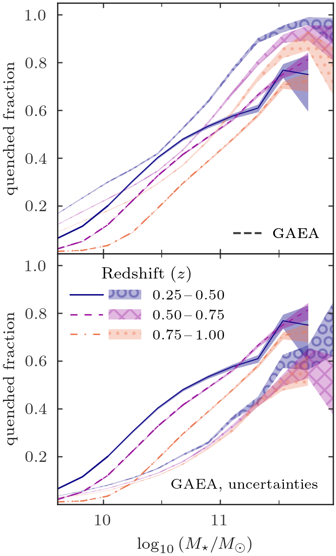
Figure 8: Top: Quenched fractions as in Fig. 1 in lines, with quenched fractions from the GAEA semi-analytic model (De Lucia et al. 2024) in hatched regions. Bottom: Quenched fractions as in Fig. 1 in lines, with quenched fractions from GAEA with Euclid-like uncertainties added in hatched regions. Including uncertainties lowers the GAEA quenched fractions considerably, explaining in part why our quenched fractions are lower than those in the literature.

In the last redshift bin, we can compare our results with the ETG fractions from seven clusters observed with the Hubble Space Telescope at $0.8<z<1.3$ from Postman et al. (2005) in Fig. 6. We note that these fractions are not separated by stellar mass, and so we plot our ETG fraction for all stellar masses. The galaxies in Postman et al. (2005) were selected at roughly the same depth as ours. Here, we see that the Postman et al. (2005) ETG fractions are generally about $10\,\%$ larger than what we find, yet consistent within uncertainties. Given that galaxy densities are calculated at the same depth and with the same method, this discrepancy might be due to the different morphological classification, which is performed based on visual morphology in Postman et al. (2005), compared to the Sérsic index-colour plane in Euclid Collaboration: Quilley et al. (2025). It is evident that, since the classification method we use has a colour cut, we might be missing some visually classified ETGs, i.e., if they have lower Sérsic index or bluer colours. Another aspect to consider is that we do not probe high galaxy densities, such as those probed in Postman et al. (2005). In fact, at $\Sigma_{7}>500\ \text{gal}\ \text{Mpc}^{-2}$ we have fewer galaxies and the error bars are too large to say anything conclusive.

We further illustrate the interplay between the stellar mass and the local density in Fig. 7, where most of the high-mass galaxies are already ETGs even at high redshift. The transformative effect of the environment can be seen, and it is much stronger at lower redshifts compared to higher redshifts, and in lower stellar-mass galaxies.

We quantify these trends described in Sec. 3.1 and 3.2 in Appendix A, by plotting the differential change in the quenched fraction and the ETG fraction due to the environment, in fixed stellar mass and redshift bins. We confirm that the differential change in the quenched fraction/ETG fraction decreases at all stellar masses at $z>0.7$, and that the environmental effect is strongest for the lowest mass galaxies at low redshifts.

Additionally, we run a Monte Carlo test 1000 times, using the uncertainties in the local density to verify if these results persist. These figures for the quenched fraction and the ETG fraction are shown in Appendix B. The trends with stellar mass and density do not change, however we observe that the fraction of quenched galaxies drops at higher stellar masses and higher densities.

4 Discussion and summary

4.1 The impact of uncertainties on our results as estimated from simulations

Currently, the Euclid data products present large uncertainties. Specifically, there are significant uncertainties in the stellar mass and SFR estimates from NNPZ, and also in the photo-$z$s from Phosphoros. Here, we examine the impact of those uncertainties on our results by using simulations. For this, we use a lightcone from the Galaxy Evolution and Assembly semi-analytic model (GAEA, De Lucia & Blaizot 2007; Hirschmann et al. 2016; Xie et al. 2017; De Lucia et al. 2024).

This model originally aimed to study the evolution of brightest cluster galaxies (BCGs), uncovering the hierarchical nature of these objects. Since the original formulation of De Lucia & Blaizot (2007), there have been several additions, including improved treatment of stellar feedback, an updated AGN feedback model, and treatment of satellite galaxies (Hirschmann et al. 2016; Fontanot et al. 2020; Xie et al. 2020; De Lucia et al. 2024). In this model, galaxies are assigned an instantaneous sSFR, and are then quenched according to a threshold in sSFR, such that $\text{sSFR}<0.3\,t_{\text{H},z}^{-1}$. Note that this is the same way we select passive galaxies in this work. We select the same sample of galaxies, using the same redshift, stellar mass, and magnitude constraints.

There are no uncertainties reported in the GAEA dataset. In order to understand the impact of the uncertainties in Euclid data on our results, we must assign uncertainties to the GAEA data. To do this, we begin with the distribution of uncertainties in photometric redshift, stellar mass, and SFR from Euclid, in narrow bins. For the stellar mass and the SFR, these uncertainties are on the logarithmic quantities. We then bin the GAEA values according to the same bins as the Euclid data. The median uncertainty and standard deviation of the Euclid uncertainties in each bin are used to construct a Gaussian distribution, from which a value is randomly chosen as the uncertainty. This value is either added or subtracted to the GAEA quantity, resulting in a new value which is representative of a real value with observational uncertainty. From this we select passive galaxies in the same way as before, except now the new value for sSFR contains observational-like uncertainties in the stellar mass and the SFR.

The quenched fractions for the original GAEA model, and for the GAEA data with uncertainties, are shown in Fig. 8, in the top and bottom panel respectively. In the top panel, it is clear that due to the uncertainties in Euclid data, the quenched fraction is underestimated compared to GAEA. Further, when we plot the GAEA-with-uncertainties data, the quenched fraction for these results is ($\sim 20$–$40\%$ lower). Of the uncertainties on redshift, stellar mass, and SFR, they each individually have a significant effect on the quenched fraction. That said, by testing different combinations of including/excluding the uncertainties, it is clear the uncertainties on the SFR dominate in determining the quenched fractions. This result underlines the importance of future data to reduce the uncertainties on galaxy physical properties. Improved processing methods on the photometric redshifts, along with an increased observing area, will help reduce uncertainties and increase statistics. In particular, we expect to find a higher number of high-density environments. For this paper we only use the simulations to examine the impact of the uncertainties on our results; that said, we do find evidence of an environmental effect on the passive fraction of massive galaxies up to $z\sim 2$ in the GAEA simulations (Cleland in prep.).

4.2 Comparing to other results

In this paper, we have showcased the early capabilities of the Euclid project, in terms of galaxy evolution and identifying a wide range of environments. Here, we identify and analyse the passive-density and morphology-density relations from $z=0.25$ to $z=1$. Many previous studies have examined quenched fractions and ETG fractions as functions of stellar mass and environment, however not all of them probe the effect of the environment at fixed stellar mass, and as a function of redshift. Our approach allows to quantify the effect of the environment for each stellar mass and redshift bin. This approach is similar to that in Peng et al. (2010), which demonstrated the separability of the effects of stellar mass and environment at $z<0.2$. This paper also found that these effects are separable to $z\sim 1$, however only in density quartiles. We have now shown on a continuous scale of density and stellar mass how the differential effects change with redshift. Similarly, while previous studies such as Postman et al. (2005); Lemaux et al. (2019); Mei et al. (2023) showed these relations at $z\sim 1$, we have expanded on these results by including a wider range of environments, as opposed to targeting overdense regions.

In Fig. 2, we find the quenched fraction of galaxies increases with increasing local density at all stellar masses, except at $z>0.75$, where only the most massive galaxies are affected by the environment, in terms of star formation. This is consistent with the results of many studies (Cucciati et al. 2017; Strazzullo et al. 2019; van der Burg et al. 2020; Baxter et al. 2023; Shi et al. 2024; Taamoli et al. 2024; Trudeau et al. 2024), however, quantitatively, the values of the quenched fractions differ slightly. As already shown in Fig. 1, the ORELSE survey (Lemaux et al. 2019) finds higher quenched fractions than our results, in almost all stellar mass and redshift bins. Yet, in Fig. 2, when we plot these fractions as a function of density, the ORELSE quenched fractions evolve very little across the density bins and the redshift bins. In these redshift bins the ORELSE quenched fractions show little difference between the stellar mass bins, whereas ours depend on the stellar mass as well as the local density. That said, as discussed in Sec. 4.1, the large uncertainties present in Euclid data products make it difficult to draw quantitative conclusions. Although, other papers with results from this redshift range show how the quenched fraction of galaxies depends strongly on the stellar mass and the environment (e.g., Davidzon et al. 2016; Weaver et al. 2023).

On the other hand, quenched fractions presented in the CARLA study (Mei et al. 2023) reach $>60\,\%$ in the highest-density environments. However, it must be noted that these results are for $1.3<z<1.9$, and so caution must be taken when directly comparing these results. Nonetheless, our quenched fractions should be higher at $z\sim 1$ than those in Mei et al. (2023) in the same mass bins used; only galaxies at $M_{\ast}>10^{11}\ M_{\odot}$ reach quenched fractions of $60\,\%$. It should also be noted that the CARLA results show little dependence on stellar mass, possibly because of the high uncertainty on their mass measurements, where our results and other studies show significant mass dependence at fixed local density. For instance, it has been shown that the environmental quenching efficiency increases with decreasing redshift, and this effect is strongest at low stellar masses (Cucciati et al. 2010, 2017; Lemaux et al. 2019), which is consistent with our results in Fig. 2.

For ETGs, we find that massive galaxies $\left(M_{\ast}>10^{11}\ M_{\odot}\right)$ are $>80\,\%$ ETGs at $z<1$. For low-mass galaxies, there is a considerable effect from the environment on their morphology at $z<0.75$. At $z>0.75$, the effect is weaker. There are many studies that show that the morphology-density relation is already in place by $z\sim 1$ (Postman et al. 2005; Shi et al. 2024), or even at $z\sim 2$ (Sazonova et al. 2020; Mei et al. 2023). In Sazonova et al. (2020) the effect is stronger at low $M_{\ast}$, which is also seen in this work. However, our ETG fractions plotted in Fig. 5 seem to be slightly underestimated compared to Postman et al. (2005) at $z\sim 1$, yet consistent within error bars. It is difficult to say anything conclusively about the densest environments due to the very small number of galaxies with $\Sigma_{7}\gtrsim 500\ \text{gal}\ \text{Mpc}^{-2}$. Qualitatively speaking, there is evidence of a morphology-density relation at $0.75<z<1$ across all stellar masses, and more prominent at $M_{\ast}<10^{10.5}\ M_{\odot}$.

In a future paper, we will extend this work to $z>1$, and include results from other high-redshift studies to compare. We will also compare to simulated Euclid data from various different galaxy evolution models (Cleland in prep.).

The first Euclid results provide observations, redshifts, and physical properties of at least one million galaxies in a wide variety of environments. With the upcoming release of DR1, the number of observed sources and the number of high-density environments in Euclid data will increase by orders of magnitude.

Appendix A Quantifying the effect of the environment

Here we quantify the differential effect of the environment in fixed stellar mass or redshift bins. The differential effect here is defined as the slope of the fitted line of the quenched fraction as a function of increasing density in stellar mass or redshift bins. This allows us to quantify the effect of the environment, and identify overall trends between low and high mass, and between low and high redshift. The results of this analysis are plotted in Fig. 9.

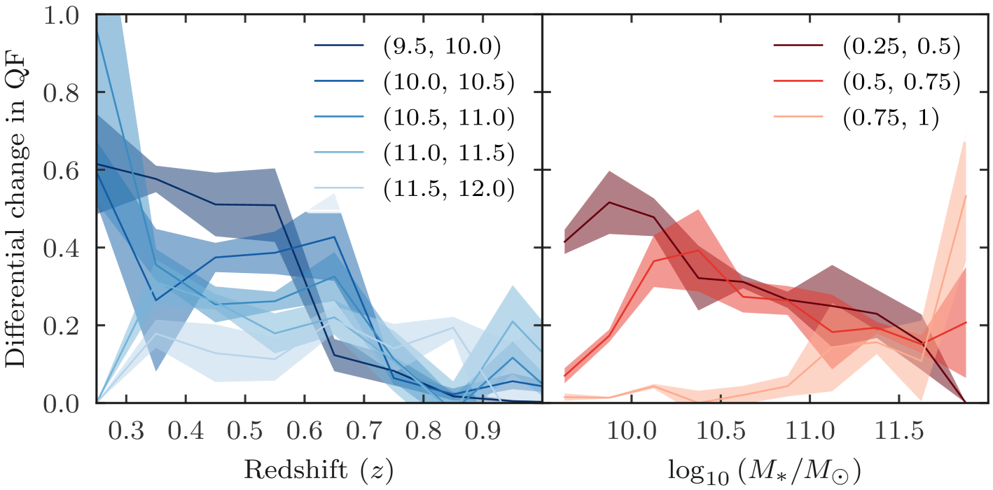
Figure 9: Left: Differential change in the quenched fraction because of the environment, as a function of redshift in fixed mass bins. The environment has the strongest effect at low-mass, and this effect is lessened with increasing redshift. Right: Same as the left panel, but as a function of stellar mass in fixed redshift bins. At low redshift, low-mass galaxies are most affected, and this effect weakens at high mass, while at high redshift, the effect increases slightly with increasing stellar mass. Shaded regions show the $1\ \sigma$ uncertainty on the slope

In the left panel Fig. 9, we see the differential change in the quenched fraction as a function of redshift, in fixed stellar mass bins. We see that at low redshift, the effect of the environment becomes stronger with decreasing stellar mass. This effect drops off at $z\sim 0.7$. In the right panel of Fig. 9, we plot the same thing but as a function of stellar mass, in fixed redshift bins. These are the same redshift bins used in the main text, however when increasing the number of bins, the main results remain the same. Again we see that at $z<0.75$, the environmental effect is strongest at low mass, and decreases with increasing mass. At $0.75<z<1$, the differential environmental effect is on average lower than in the other two redshift bins, however there is evidence that the environmental effect actually increases at high mass here. That said, the uncertainty on the slope is large.

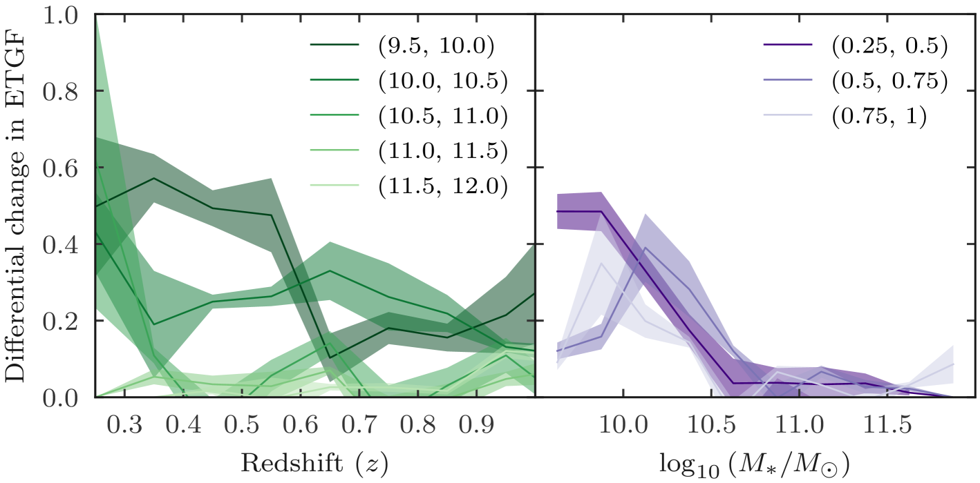
Figure 10: Same as Fig. 9 but for the ETG fraction.

We plot the same thing but for the ETG fraction in Fig. 10. The main difference here is that the differential change on the ETG fraction due to the environment is very low at $M_{\ast}>10^{10.5}\ M_{\odot}$. Again, we see that, at low redshift, the environmental effect is strongest for low-mass galaxies.

Appendix B Monte Carlo tests

We present the results of our Monte Carlo experiments, after 1000 runs. For each realisation, we draw a value from a Gaussian distribution, centered on $\Sigma_{7}$ and with the uncertainty on $\Sigma_{7}$, as described in Sect. 2.2, as the standard deviation of the distribution. This results in a perturbed value for the local density. We use this perturbed value to create the same binned plots in Figs. 3 and 7. After 1000 realisations, we take the mean value in each bin to obtain a ‘smoothed’ version of the results in the main text. This procedure allows us to identify if the trends persist after taking into account the uncertainties on the density measurements.

In Fig. 11, we see that for the quenched fraction, the dependence on both stellar mass and environment at $z<0.75$ remains, although the quenched fraction is reduced in regions of the plot where there were very few galaxies (high stellar mass and high local density). At $z>0.75$, the stellar mass is the dominant factor in determining the mean quenched fraction, with only a very slight dependence on environment.

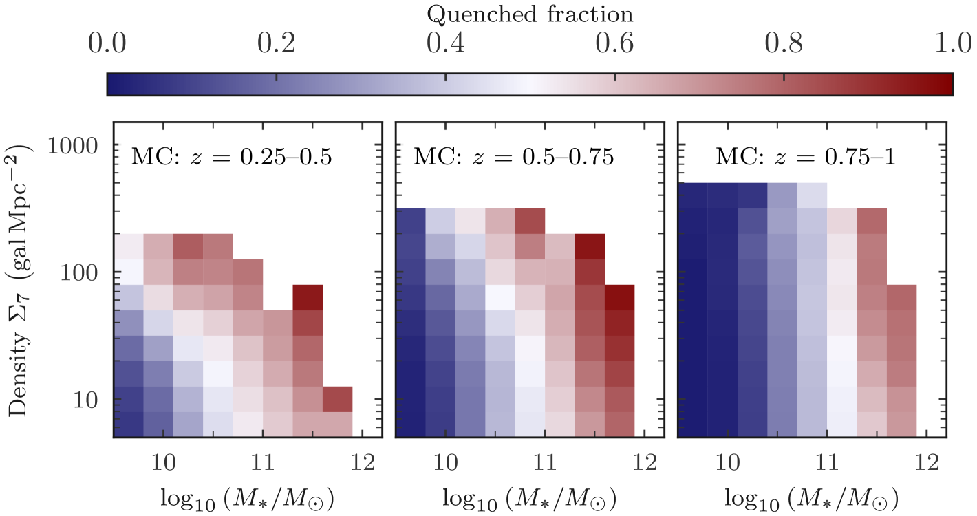
Figure 11: Same as Fig. 3, but after 1000 Monte Carlo tests run to show the dependence of the quenched fraction on environment and stellar mass.

For the ETG fraction, in Fig. 12, the result that the environment has the biggest effect on low-mass galaxies at $z<0.5$ is still visible. The ETG fraction depends strongly on the stellar mass in all redshift bins. At $0.5<z<0.75$, the ETG fraction depends less on the environment, but the effect is still there at $M_{\ast}<10^{10.5}\ M_{\odot}$. At $z>0.75$, there is very little evidence that the ETG fraction depends on environment.

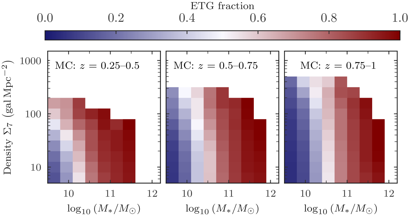
Figure 12: Same as Fig. 7, but after 1000 Monte Carlo tests run to show the dependence of the ETG fraction on environment and stellar mass.