Active Leakage Cancellation in Single Qubit Gates

Active Leakage Cancellation in Single Qubit Gates

Abstract

The ability to perform fast and accurate rotations between the computational basis states of quantum bits is one of the most fundamental requirements for building a quantum computer. Because physical qubits generally contain more than two levels, faster gates often result in a higher leakage rate outside of the computational space. In this letter, we enhance the state-of-the-art single qubit gate by introducing active leakage cancellation. This is accomplished via a second drive tone near the leakage transition such that we cancel the leakage caused by the main drive. Furthermore, we describe a measurement sequence that can be used to calibrate the parameters of this leakage cancellation drive. Finally, we apply the technique to superconducting transmon qubits, suppressing the leakage below the $10^{-5}$ level, and achieving coherence-limited gate infidelity of $7.5\times 10^{-5}$, for a 10 ns $\pi/2$ gate and 196 MHz qubit anharmonicity.

I Introduction

While below-threshold quantum error correction (QEC) performance has been demonstrated recently [1, 2, 3], further advancement towards practical quantum computing requires improving the performance of quantum gates for the underlying physical qubits. Weakly anharmonic qubits such as the superconducting transmon qubits [4, 5, 6, 7, 8, 9], have transition frequencies for $\ket{0}\rightarrow\ket{1}$ and $\ket{1}\rightarrow\ket{2}$ relatively close to each other. These qubits face a fundamental tension in gate optimization. On the one hand, it is desirable to make the operations as fast as possible to minimize the impact of decoherence. On the other hand, as gate length is reduced, spectral power from the driving field is increasingly delivered to the undesired transition from $\ket{1}$ to $\ket{2}$, causing leakage to outside the computational space to be increasingly likely. Recent studies show that leakage accumulation is particularly detrimental to QEC [10].

There have been many attempts to engineer the spectrum of the control pulse near the frequency $f_{21}$ of the unwanted transition from state $|1\rangle$ to $|2\rangle$ to reduce the resulting leakage. Of particular note is Derivative Removal by Adiabatic Gate (DRAG), which produces a spectral notch at the specified frequency by adding a quadrature component to the control envelope [11, 12, 13, 14, 15]. More recently, Fourier ansatz spectrum tunning (FAST) has been developed to further reduce power near $f_{21}$ with a control envelope that comprises a linear combination of higher harmonics of the base cosine envelope [16]. While FAST has been shown to suppress leakage beyond standard cosine pulse with DRAG, it requires the use of higher harmonics, therefore more stringent on the sampling rate of the pulse generator.

In this work, we introduce a simple yet quite powerful control strategy to suppress leakage in single qubit gates, that is applicable to all qubit systems supporting levels in addition to computational basis states, in particular to systems that have low anharmonicity. Our strategy is to implement an active leakage cancellation (ALC) drive signal at the dominant leakage transition frequency $f_{21}$, simultaneous with the primary drive, that cancels the leakage caused by the main drive. We demonstrate this simple technique using superconducting transmon qubits and achieve 10 to 20 fold reduction in leakage per single qubit $\pi/2$ gate, compared to standard DRAG, across qubits with low (158 MHz) to moderate (196 MHz) anharmonicity. For a qubit with this moderate anharmonicity, we push the leakage below $10^{-5}$ for a 10 ns $\pi/2$ gate, compared to $10^{-4}$ using only DRAG.

Our active leakage cancellation strategy is extremely effective in cancelling the leakage, while at the same time preserving the spectrum and power of the primary pulse near the intended transition frequency; see Fig. 1. In contrast to FAST [16] and higher-derivative DRAG [17], our leakage cancellation drive does not increase the pulse spectral power far away from the leakage transition, bandwidth of the pulse remains confined. Furthermore, applying the leakage cancellation drive has less stringent requirement on the sample rate compared to FAST.

While pulse shaping techniques often require complex calibration/optimization procedure [18], our active leakage cancellation strategy does not add significant calibration overhead. The leakage cancellation drive only adds two additional parameters (amplitude and frequency of the pulse) to the overall pulse envelope and they can be calibrated independent of the primary drive. We employ a Ramsey filter technique [19] to amplify coherent leakage which is then used as a metric to optimize the cancellation drive parameters.

Figure 1: Pulse envelope of active leakage cancellation (ALC) drive, example shown for $\eta=200$ MHz and a 9.5 ns $\pi/2$ gate. a) Time-domain pulse envelope components. Real part of the primary drive (solid, blue) follows a raised-cosine pulse shape, and the imaginary part (dashed, blue) results from the application of DRAG. The composite pulse (primary + active leakage cancellation drive) is shown in gold. b) The spectra of the pulse envelope for the basic raised cosine with DRAG (blue), and with added leakage cancellation (gold) over a 2 GHz band centered about $f_{10}$. Vertical dashed lines indicate transition frequencies $f_{21}$ (red) and $f_{10}$ (green). Inset shows the level diagram of a transmon qubit. c) qubit states $|0\rangle$ (blue), $|1\rangle$ (green) and $|2\rangle$ (red) and $|3\rangle$ (purple) populations during the gate operation using DRAG only (dashed) vs using DRAG and active leakage cancellation (solid), for qubit initial state in $|0\rangle$ (left) and $|1\rangle$ (right). Final population in state $|2\rangle$ is substantially reduced by using DRAG + ALC compared with using DRAG only.

II Pulse shaping and modeling

Active leakage cancellation is a technique with general applicability to a variety of physical platforms. Here, for clarity, we discuss the pulse shaping and modeling of the leakage cancellation drive for the specific case of transmon qubits.

We model a transmon qubit as a Kerr nonlinear oscillator [20]. Its Hamiltonian is given by $H_{q}/h=f_{10}a^{\dagger}a-\eta a^{\dagger 2}a^{2}/2$ where $a,a^{\dagger}$ are bosonic ladder operators, $f_{10}$ is the qubit transition frequency from state $\ket{0}$ to $\ket{1}$, $\eta$ is the anharmonicity that sets the difference between transition frequency from $\ket{2}$ to $\ket{1}$ and $\ket{1}$ to $\ket{0}$: $\eta=f_{10}-f_{21}$. For transmon qubits, we have $\eta>0$ and $\eta\ll f_{10}$. To describe the dynamics in the presence of microwave drives, we switch to the frame that rotates at the qubit frequency $f_{10}$. Under the rotating wave approximation, the rotating-frame Hamiltonian reads (see Appendix A for the lab-frame Hamiltonian):

$$H(t)/h=-\frac{\eta}{2}\hat{a}^{\dagger 2}\hat{a}^{2} +\frac{1}{2}\left[\Omega_{\rm main}(t)+\Omega_{\rm alc}(t)\right]\hat{a}$$

$$+\frac{1}{2}\left[\Omega_{\rm main}^{*}(t)+\Omega_{\rm alc}^{*}(t)\right]\hat{a}^{\dagger},$$ (1)

where $\Omega_{\rm main}(t)$ and $\Omega_{\rm alc}(t)$ refer to the complex envelope of the primary drive and active leakage cancellation drive, respectively. In all equations, we use lower-case “alc” to indicate active leakage cancellation pulse.

Our implementation of the primary control envelope is the same as in Ref. [15]. As in the standard DRAG scheme, we take the primary control envelope to be real valued in the rotating frame of the qubit, and introduce a notch in the spectrum of the control pulse at $f_{21}$ by adding a quadrature component proportional to the derivative of the in-phase component:

$$\Omega_{\rm main}(t)=A_{\rm main}\left[F(t)+i\frac{\alpha}{2\pi\Delta}\frac{dF(t)}{dt}\right]e^{i2\pi\delta_{\rm main}t},$$ (2)

where $A_{\rm main}$ refers to the amplitude of the primary drive and $\delta_{\rm main}$ refers to the detuning of the drive frequency $f_{\rm main}$ from $f_{10}$, i.e., $\delta_{\rm main}=f_{\rm main}-f_{10}$. A small detuning is needed to compensate the ac Stark shift induced by the drive [15]. In this work, we fix the DRAG parameter $\alpha$ to be 1 to minimize leakage. Parameter $\Delta$ sets the position of the notch and is fixed to be $\Delta=-\eta-\delta_{\rm main}$. In the data presented in this letter we consider the common choice of a raised cosine envelope for single qubit gates,

$$F(t)=1-\cos\left[2\pi\frac{t+t_{\rm gate}/2}{t_{\rm gate}}\right],$$ (3)

which starts at $t=-t_{\rm gate}/2$ and ends at $t=t_{\rm gate}/2$.

Whereas in DRAG, we suppress the spectrum of the drive pulse near $f_{21}$ by adding a quadrature component at the same frequency as the primary drive, our implementation of the leakage cancellation introduces an additional drive tone with frequency very close to $f_{21}$. The drive envelope of the additional tone is described by the following:

$$\Omega_{\rm alc}(t)=iA_{\rm alc}\frac{1}{2\pi\delta_{\rm alc}}\frac{dF(t)}{dt}e^{i2\pi\delta_{\rm alc}t}.$$ (4)

Parameter $A_{\rm alc}$ quantifies the amplitude of the leakage cancellation drive whereas $\delta_{\rm alc}$ is the detuning of the drive frequency $f_{\rm alc}$ from qubit $f_{10}$, i.e., $\delta_{\rm alc}=f_{\rm alc}-f_{10}$. We optimize these parameters to minimize leakage; see Sec. III. Typically we have $\delta_{\rm alc}\approx-\eta$, and amplitude $A_{\rm alc}$ is $\sim 10\%$ to 20$\%$ of the main pulse amplitude $A_{\rm main}$ with an opposite sign, for gates between $\sim 10$ and 15 ns. In a way, the leakage cancellation drive is similar to the DRAG term of the main drive, but is shifted in frequency by approximately $-\eta$. As we will see in Eq. (6), the leakage cancellation drive itself has a notch near $f_{21}$. When combined with DRAG, it strongly suppresses leakage.

Figure 1 illustrates the construction of the leakage cancelled gate for the case $F(t)$ given by Eq. (3), $\eta=200$ MHz, and $t_{\rm gate}=9.5$ ns. Pulse parameters are numerically optimized to give the lowest error for a $\pi/2$ gate. In Fig. 1(a), shown in blue is the time domain control envelope of the main drive optimized in the absence of the leakage cancellation drive. The real part of this envelope (solid) is due to the raised cosine profile while the imaginary part (dashed) results from the application of DRAG. The gold lines in Fig. 1(a) show the composite pulse envelope including the leakage cancellation drive. We numerically verified that the addition of the leakage cancellation drive only weakly changes the optimal parameters for the main pulse. Furthermore, the strength of the leakage cancellation drive is weak compared to the main drive, as indicated by the small difference between main and the composite drive. Unlike the main drive envelope, the composite envelope is not a simple sine wave. This is because the additional leakage cancellation drive has modulation at frequency $\delta_{\rm alc}$ on top of the raised cosine envelope.

Figure 1(b) shows the spectra of the pulse envelopes, computed as the Fourier transform of the time-domain pulse. It follows from Eqs. (2, 4) that the spectra of the primary and leakage cancellation drive are given by:

$$\Omega_{\rm main}[f] =A_{\rm main}\left[1-\frac{\alpha}{\Delta}(f-\delta_{\rm main})\right]F[f-\delta_{\rm main}],$$ (5)

$$\Omega_{\rm alc}[f] =A_{\rm alc}\left[1-\frac{1}{\delta_{\rm alc}}f\right]F[f-\delta_{\rm alc}],$$ (6)

where $\Omega_{\rm main}[f]\equiv\int_{-\infty}^{\infty}\Omega_{\rm main}(t)e^{-i2\pi ft}dt$, $\Omega_{\rm alc}[f]\equiv\int_{-\infty}^{\infty}\Omega_{\rm alc}(t)e^{-i2\pi ft}dt$, and $F[f]\equiv\int_{-\infty}^{\infty}F(t)e^{-i2\pi ft}dt$. In our implementation, we fix $\alpha=1$, and $\Delta=-(\eta+\delta_{\rm main})$ such that spectrum $\Omega_{\rm main}[f]$ has a spectral notch at $f=-\eta$. The leakage cancellation drive itself has a notch at $\delta_{\rm alc}$ which is close to but often not exactly at $-\eta$. Compared to the spectrum of the main drive (DRAG only, blue), the composite pulse (DRAG + ALC, gold) has a larger spectral weight few hundreds of MHz below leakage transition $f_{21}$. However, farther away from $f_{21}$, in particular, near the intended transition $f_{10}$, the spectrum is only weakly perturbed compared to without leakage cancellation drive.

Figure 1(c,d) show numerically simulated qubit state populations during the gate, for qubit initially in state $|0\rangle$ and $|1\rangle$, respectively. While state $|2\rangle$ population during the gate is similar between pulses with only DRAG and with DRAG plus leakage cancellation, the final population in state $|2\rangle$ is reduced by several orders of magnitude by applying the active leakage cancellation. Final population in state $|3\rangle$ is somewhat higher in DRAG + ALC, but it is still few orders of magnitude smaller than state $|2\rangle$ population in the case of DRAG only. In essence, the leakage cancellation drive very effectively cancels the $|2\rangle$ state leakage amplitude through destructive interference by fine tuning its frequency around $f_{21}$ and its amplitude.

III Calibration

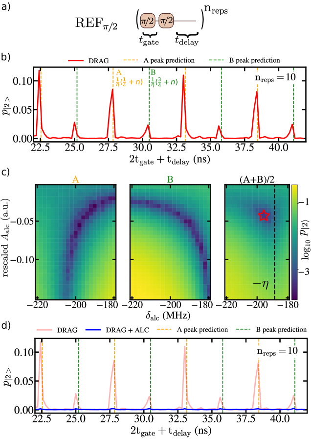
Figure 2: Calibration sequence for leakage cancellation parameters. a) The pulse sequence for the $\rm REF_{\pi/2}$. b) Example data from the $\rm REF_{\pi/2}$ for the case of $n_{\rm reps}=10$, the peaks are due to the amplification of coherent leakage induced by the $\pi/2$ pulses. c) Optimization of leakage cancellation drive amplitude $A_{\rm alc}$ and detuning $\delta_{\rm alc}$. The left and center panels are acquired at two different $t_{\rm delay}$, one at an A peak, and the other at a B peak shown in panel b), the right panel shows the average leakage population $p_{|2>}$. The optimal leakage cancellation parameters are indicated by the red star where the average of leakage contributions from A and B are minimized. The optimal $\delta_{\rm al}$ is slightly shifted from $-\eta$ (vertical dashed line). d) Uncompensated data (red) from the $\rm REF_{\pi/2}$ from panel (b) (red) compared with the $\rm REF_{\pi/2}$ with active leakage cancellation (blue) showing suppression of coherent leakage.

In this section we detail a calibration procedure that can be used to experimentally determine the optimal leakage cancellation parameters. Our calibration sequence employs the Ramsey error filter (REF) technique to amplify the coherent leakage produced by the control pulse [19]. The pulse sequence for the $\pi/2$ variant of the Ramsey error filter REF_π/2 is shown in Fig. 2(a). The $\pi/2$ pulses drive a small population from $\ket{1}$ to $\ket{2}$ while the Ramsey delay $t_{\rm delay}$ allows for phase accumulation in the $\ket{1}$, $\ket{2}$ subspace. This phase accumulation allows the constructive interference between the pulse unitaries and thus population coherently accrues into the $\ket{2}$ state. This sequence is repeated $n_{\rm reps}$ times to amplify the population transfer.

In Fig. 2(b), we show the observed $\ket{2}$ population $p_{\ket{2}}$ vs $t_{\rm delay}$ during the Ramsey error filter experiment. Peaks in $p_{\ket{2}}$ correspond to the satisfaction of a constructive interference condition: $\eta(4t_{\rm gate}+2t_{\rm delay})=(k+1/2)$, with $k=0,1,2..$. This condition can be understood as that every four $\pi/2$ pulses complete a cycle in which the qubit goes from $\ket{0}$ to $\ket{1}$ and returns to $\ket{0}$ with a $\pi$ phase shift, and to have constructive interference in the amplitude of state $\ket{2}$ from cycle to cycle, we need to have $\eta$ multiplied by the cycle time $(4t_{\rm gate}+2t_{\rm delay})$ to be half of odd integer. The peaks corresponding to $k$ being even ($k=2n$) and odd integer ($k=2n+1$) can in general be different, they are referred to as type-A and type-B peaks, respectively, in Fig. 2(b). Their heights are determined by the interference of amplitude transfer to state $\ket{2}$ within a cycle (between first and second half of a cycle), thus are different for different $\eta(2t_{\rm gate}+t_{\rm delay})$ modulo 1.

Figure 2(c) shows the two-parameter optimization of the leakage cancellation parameters. In the left subpanel, we show the observed $p_{\ket{2}}$ with $t_{\rm delay}$ held fixed at the value that maximizes $p_{\ket{2}}$ for a type A peak. In the center subpanel, we show the analogous data for a peak of type B. A naive optimization might attempt to minimize the population in either an A peak or a B peak, however this approach generally fails. This is because although the targeted peak may be minimized, peaks of the other type may be enhanced in the process. In the right-most panel of Fig 2(c), we show the average $p_{\ket{2}}$ in the A and B peaks vs $A_{\rm alc}$ and $\delta_{\rm alc}$. The red star indicates the optimal leakage cancellation drive parameters. As expected, the optimal detuning is near $-\eta$. In Fig. 2(d), we show validation data (blue) demonstrating that this choice of cancellation parameters suppresses leakage from the $\pi/2$ gates for all values of $t_{\rm delay}$.

IV Demonstration

Figure 3: Randomized benchmarking of single qubit gates with active leakage cancellation, for qubits with $\eta=$ 158 MHz ($f_{10}=4.5$ GHz) and 196 MHz ($f_{10}=5.7$ GHz). a) and b) The leakage rate for gates constructed with DRAG only (solid markers) and with both DRAG and ALC (hollow markers) as observed through RB sequences. Measured leakage rates agree well with numerical predictions (lines) of coherent leakage with an additive offset representing a background leakage largely due to heating. c) and d) Average gate error as assessed by RB. The numerical prediction (lines) reflects the gate error through the leakage channel plus error from qubit decoherence due to $T_{1},T_{\phi}$ (black dotted line). The latter uses formula, gate error = $t_{\rm gate}/3T_{1}+t_{\rm gate}/3T_{\phi}$ with independently measured $T_{1}$ and $T_{\phi}$ [panel (c): $T_{1}$ = 104 ${\rm\mu s}$, $T_{\phi}$ = 118 ${\rm\mu s}$; panel (d) $T_{1}$ = 101 $\mu s$,$T_{\phi}$ = 109 ${\rm\mu s}$] In panel (c), the result from the formula is multiplied by a factor of 1.3 to match the data indicating additional decoherence during the gate compared to idle. In panel (d), the formula matches well the measured error at long gate times without correction. e) and f) state $\ket{2}$ population and RB fidelity as a function of gate depth for $t_{\rm gate}=9.75$ ns and $\eta=196$ MHz. Figure legend indicates leakage probability per cycle $\Gamma_{\uparrow}$ and RB error $r$.

We demonstrate our technique on qubits with 158 MHz and 196 MHz nonlinearity, using a 1 GS/s AWG that is up-converted to the qubit frequency. Figure 3 shows the performance of $\pi/2$ gates vs $t_{\rm gate}$ for gates with and without leakage cancellation. For each gate length, we first calibrate the parameters of the primary drive, without leakage cancellation, including the drive amplitude, detuning from $f_{10}$, and a post-gate phase correction. Once the primary drive has been calibrated, we calibrate the amplitude and detuning of the active leakage cancellation drive using the procedure detailed in the previous section. Finally, we re-calibrate the primary drive parameters in the presence of the leakage cancellation drive.

Figure 3(a,b) compare the leakage probability per gate with and without leakage cancellation, as characterized by randomized benchmarking (RB). While the leakage rate generally increases with the decrease in the gate time, without leakage cancellation (solid markers), the leakage rate increases beyond the $10^{-5}$ level approximately at $t_{\rm gate}\approx 2.5/\eta$, this corresponds to $t_{\rm gate}\approx 16$ ns for $\eta=158$ MHz, and 13 ns for $\eta=196$ MHz. With leakage cancellation (hollow markers), we push this to a significantly smaller gate time of $t_{\rm gate}\approx 1.9/\eta$, approximately $t_{\rm gate}\approx 12$ ns for $\eta=158$ MHz, and 9.7 ns for $\eta=196$ MHz. Compared with the leakage rate without leakage cancellation at the same gate times, we achieved up to a factor of 20 reduction in the leakage rate through the leakage cancellation drive. The experimental leakage rate is limited by an incoherent heating rate of approximately 5 $\times 10^{-6}$ per gate, without which we expect even stronger reduction of the leakage through the leakage cancellation drive.

Figure 3(c,d) compare the average gate error with and without leakage cancellation. At relatively long gate times, the gate error is limited by qubit decoherence (black dotted lines) and scales approximately linearly with gate duration. At short gate times, gate error increases due to the increase in the coherent leakage. In the regime where the gate fidelity is strongly impacted by coherent leakage we observe a significant reduction in the error rate with leakage cancellation applied. For $\eta=158$ MHz, we achieve a gate error of $1.3\times 10^{-4}$ at $t_{\rm gate}=12$ ns, compared to $3.1\times 10^{-4}$ at the same gate time using DRAG alone, which is a factor of 2.4 reduction. We attribute this improvement to the 12x reduction in leakage, from $1.8\times 10^{-4}$ to $1.5\times 10^{-5}$, that results from applying ALC. Similarly, for $\eta=196$ MHz with $t_{\rm gate}=9.75$ ns, we observe a 16x reduction in the leakage rate from $1.5\times 10^{-4}$ without ALC to $9.2\times 10^{-6}$ with ALC with a concomitant improvement in the gate error from $2.3\times 10^{-4}$ without ALC to $7.9\times 10^{-5}$ with ALC, a factor of 2.9 reduction. With ALC, the lowest gate error we observe is $7.5\times 10^{-5}$ at $t_{\rm gate}=10$ ns, which is primarily coherence limited. For both values of $\eta$, leakage cancellation permits a higher fidelity gate than would be possible with DRAG alone.

Figure 3(e,f) highlight the leakage population and RB fidelity as a function of gate depth at $t_{\rm gate}=9.75$ ns for $\eta=196$ MHz. The improvement in both gate fidelity and leakage rate through the active leakage cancellation drive persists at large gate depths.

Numerical results in Fig. 3 are obtained by simulating the rotating-frame Hamiltonian in Eq. (II). It uses the same iterative procedure to optimize the primary and leakage cancellation drive parameters independently, as followed in the experiment. The simulated leakage rate agrees quite well with experiments as shown in Fig. 3(a,b). Simulations show that a global optimization of the primary and leakage cancellation drive parameters could achieve another two to three-fold reduction in the leakage rate; see Appendix B. This suggests the possibility of further reducing the leakage seen in the experiments by improving the experimental calibration procedure (e.g. more iterative steps).

V Conclusions

We developed an active leakage cancellation strategy that significantly enhances the performance of single-qubit gates, particularly in systems with low anharmonicity. By implementing a second drive tone at the leakage transition frequency $f_{21}$, we efficiently compensate the leakage caused by the primary drive. We developed a simple calibration procedure to optimize the leakage cancellation pulse parameters. Moreover, we experimentally demonstrated this technique on superconducting transmon qubits, and achieved a 10 to 20-fold reduction in leakage compared to standard DRAG. For qubits with an anharmonicity of 196 MHz, leakage is suppressed below $10^{-5}$ for a 10 ns $\pi/2$ gate, enabling a coherence-limited gate infidelity of $7.5\times 10^{-5}$. Through further optimization of the leakage cancellation pulse shape, more sophisticated calibration procedure, or combining the technique with other pulse shaping technique such as FAST, we anticipate even stronger performance. This active leakage cancellation strategy represents a simple yet powerful approach to improving the speed and accuracy of single-qubit gates, much needed for the advancements towards practical quantum computing.

Appendix A Hamiltonian in the lab frame

In this section, we describe the Hamiltonian of the driven transmon in the lab frame.

In the presence of both primary and leakage cancellation drive, the transmon Hamiltonian in the lab frame is given by

$$H_{\rm lab}(t)/h =f_{10}a^{\dagger}a-\eta a^{\dagger 2}a^{2}/2$$

$$+\Big{[}A_{\rm main}F(t)\cos(2\pi f_{\rm main}t)$$

$$-A_{\rm main}\frac{\alpha}{2\pi\Delta}\dot{F}(t)\sin(2\pi f_{\rm main}t)$$

$$-A_{\rm alc}\frac{1}{2\pi\delta_{\rm alc}}\dot{F}(t)\sin(2\pi f_{\rm alc}t)\Big{]}(a+a^{\dagger}),$$ (7)

where $\delta_{\rm alc}=f_{\rm alc}-f_{10}$. The first two terms in the square bracket describe the primary drive and its DRAG component and the third term describes the active leakage cancellation drive. Frequencies of the main drive and leakage cancellation drive are $f_{\rm main}$ and $f_{\rm alc}$, respectively. Function $F(t)$ describes the pulse envelope. In the rotating frame at qubit frequency $f_{10}$ and under rotating wave approximation, this Hamiltonian transforms to the Hamiltonian in Eq. (II) in which $\Omega_{\rm main}$ and $\Omega_{\rm alc}$ are given by Eq. (2) and Eq. (4), respectively.

Appendix B Additional numerical simulation results

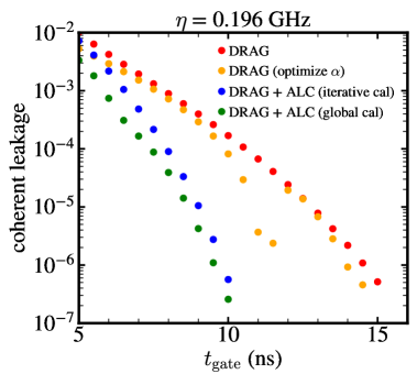
Figure 4: Numerical simulations of coherent leakage after a $\pi/2$ pulse for $\eta=0.158$ GHz (left) and 0.196 GHz (right). Markers of different colors refer to different leakage suppression strategy: red markers refer to applying only DRAG ($\alpha=1$), orange markers refer to applying DRAG with optimized DRAG parameter $\alpha$, blue and green markers refer to combining DRAG ($\alpha=1$) and active leakage cancellation but with different optimization procedure (iterative vs global); see the text for details. The leakage shown here only includes drive-induced coherent leakage into states outside of the computational subspace, and does not include additional background leakage due to heating as shown in Fig. 3(a,b). Blue and green markers greater than 13 ns (10 ns) on the left (right) panel are lower than $10^{-7}$.

In this section, we show additional numerical simulation results based on the Hamiltonian in Eq. (II). Four transmon states are included in the simulations.

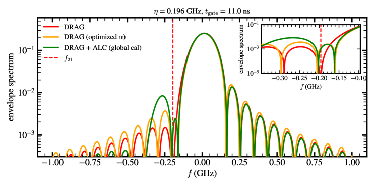
Figure 5: Spectra of pulse envelopes of different leakage suppression strategy corresponding to $\eta=0.196$ GHz (Fig. 4 right panel) at two different gate times: $t_{\rm gate}=9.5$ ns (top), $t_{\rm gate}$ = 11 ns (bottom). The spectra are centered at qubit $f_{10}$. Same color encoding as Fig. 4 are used to indicate different leakage suppression strategy. Insets show the zoomed-in spectra near $f_{21}$.

In Fig. 4, we compare coherent leakage for a $\pi/2$ pulse between different leakage suppression strategies. Coherent leakage includes the sum of final populations in states $|2\rangle$ and $|3\rangle$ at the end of the gate. Red and orange markers refer to using DRAG only with fixed DRAG parameter $\alpha=1$ and optimized DRAG parameter, respectively. Blue and green markers refer to combining DRAG (with $\alpha$ fixed at 1) and active leakage cancellation using iterative optimization and global optimization, respectively. Iterative optimization follows the same three-step procedure as used in the experiments: in step 1, we optimize the primary pulse parameters to minimize the computational space error in the absence of leakage cancellation drive; in step 2, we optimize leakage cancellation drive parameters to minimize leakage to state $\ket{2}$; in step 3, we re-optimize primary drive parameters in the presence of leakage cancellation drive. In the global optimization, we optimize pulse parameters all together to minimize the total gate error defined as the squared state overlap between the target and actual state averaged over six different initial states, $\ket{0},\ket{1},\ket{0}\pm\ket{1},\ket{0}\pm i\ket{1}$. In all the four cases, we verified numerically that the remaining gate error after the optimization is dominated by the coherent leakage. In the case of DRAG + ALC, coherent leakage generally consists of leakage to both states $|2\rangle$ and $|3\rangle$ (their relative amplitude varies with gate time), while in the case of DRAG, it mainly consists of leakage to state $|2\rangle$.

Figure 4 demonstrates substantial coherent leakage reduction by using DRAG + ALC compared with using DRAG only. Furthermore, DRAG + ALC with globally optimized primary and leakage cancellation drive parameters (green) outperforms the iterative optimization (blue) by 2 to 3 fold. Lastly, we show that simply optimizing the drag parameter $\alpha$ (orange) in the standard DRAG scheme does not achieve the same performance as DRAG + ALC. While optimizing DRAG parameter $\alpha$ reduces leakage compared with fixed $\alpha$ at certain gate times, the improvement at other gate times are marginal. Even for the gate times that show improvement, the improvement are significantly less than using DRAG + ALC.

Figure 5 compares the spectra of pulse envelopes of different leakage suppression strategies. The standard DRAG with $\alpha=1$ has a notch exactly at frequency $f_{21}$. In contrast, DRAG with optimized $\alpha$ and DRAG + ALC have notches at frequencies slightly shifted from $f_{21}$. Interestingly, in the case in which DRAG with optimized $\alpha$ shows significant improvement compared with DRAG with $\alpha$ fixed at 1, the locations of the notches almost match with those of DRAG + ALC; see the green and orange curves in Fig. 5 inset. Yet even in this case, DRAG + ALC shows substantial leakage reduction compared to DRAG with optimized $\alpha$. This indicates that to achieve the very strong leakage suppression as shown in DRAG + ALC, simply creating spectral notches near $f_{21}$ is not sufficient; rather, the leakage cancellation drive works by utilizing somewhat complicated destructive interference in the leakage amplitudes.

A comment is in order. In Fig. 4 left panel, the leakage suppression performance of DRAG + ALC (iterative cal) is better than those shown in Fig. 3 for the same anharmonicity of $\eta=158$ MHz. This is because after the experimental data in Fig. 3(a,c) were collected, we found that using $\Delta=-(\eta+\delta_{\rm main})$ for the primary pulse [see Eq. (2)] achieves better performance in the leakage cancellation (about a factor of 3 to 4 further reduction in leakage) than using $\Delta=-\eta$, which was used in Fig. 3(a,c). In Fig. 4, we show the better results using $\Delta=-(\eta+\delta_{\rm main})$; In all the results for $\eta=$ 196 MHz, we also use $\Delta=-(\eta+\delta_{\rm main})$.

References

- Google Quantum AI [2023] Google Quantum AI, Nature 614, 676 (2023).
- Google Quantum AI and Collaborators [2025] Google Quantum AI and Collaborators, Nature 638, 920 (2025).
- Putterman et al. [2025] H. Putterman et al., Nature 638, 927 (2025).
- Koch et al. [2007] J. Koch, T. M. Yu, J. Gambetta, A. A. Houck, D. I. Schuster, J. Majer, A. Blais, M. H. Devoret, S. M. Girvin, and R. J. Schoelkopf, Phys. Rev. A 76, 042319 (2007).
- Schreier et al. [2008] J. A. Schreier, A. A. Houck, J. Koch, D. I. Schuster, B. R. Johnson, J. M. Chow, J. M. Gambetta, J. Majer, L. Frunzio, M. H. Devoret, S. M. Girvin, and R. J. Schoelkopf, Phys. Rev. B 77, 180502 (2008).
- Peterer et al. [2015] M. J. Peterer, S. J. Bader, X. Jin, F. Yan, A. Kamal, T. J. Gudmundsen, P. J. Leek, T. P. Orlando, W. D. Oliver, and S. Gustavsson, Phys. Rev. Lett. 114, 010501 (2015).
- Kono et al. [2020] S. Kono, K. Koshino, D. Lachance-Quirion, A. F. van Loo, Y. Tabuchi, A. Noguchi, and Y. Nakamura, Nature Communications 11, 3683 (2020).
- Place et al. [2021] A. P. Place, L. V. Rodgers, P. Mundada, B. M. Smitham, M. Fitzpatrick, Z. Leng, A. Premkumar, J. Bryon, A. Vrajitoarea, S. Sussman, et al., Nature Communications 12, 1779 (2021).
- Lazăr et al. [2023] S. Lazăr, Q. Ficheux, J. Herrmann, A. Remm, N. Lacroix, C. Hellings, F. Swiadek, D. C. Zanuz, G. J. Norris, M. B. Panah, et al., Phys. Rev. Applied 20, 024036 (2023).
- Miao et al. [2023] K. C. Miao, M. McEwen, J. Atalaya, D. Kafri, L. P. Pryadko, A. Bengtsson, A. Opremcak, K. J. Satzinger, Z. Chen, P. V. Klimov, et al., Nature Physics 19, 1780 (2023).
- Motzoi et al. [2009] F. Motzoi, J. M. Gambetta, P. Rebentrost, and F. K. Wilhelm, Phys. Rev. Lett. 103, 110501 (2009).
- Gambetta et al. [2011] J. M. Gambetta, F. Motzoi, S. T. Merkel, and F. K. Wilhelm, Phys. Rev. A 83, 012308 (2011).
- Lucero et al. [2010] E. Lucero, J. Kelly, R. C. Bialczak, M. Lenander, M. Mariantoni, M. Neeley, A. O’Connell, D. Sank, H. Wang, M. Weides, et al., Phys. Rev. A 82, 042339 (2010).
- Chow et al. [2010] J. M. Chow, L. DiCarlo, J. M. Gambetta, F. Motzoi, L. Frunzio, S. M. Girvin, and R. J. Schoelkopf, Phys. Rev. A 82, 040305 (2010).
- Chen et al. [2015] Z. Chen, J. Kelly, C. Quintana, R. Barends, B. Campbell, Y. Chen, B. Chiaro, A. Dunsworth, A. G. Fowler, E. Lucero, E. Jeffrey, A. Megrant, J. Mutus, M. Neeley, C. J. Neill, P. J. J. O’Malley, P. Roushan, D. T. Sank, A. Vainsencher, J. Wenner, T. White, A. N. Korotkov, J. M. Martinis, and J. M. Martinis, Phys. Rev. Lett. 116 2, 020501 (2015).
- Hyyppä et al. [2024] E. Hyyppä, A. Vepsäläinen, M. Papič, C. F. Chan, S. Inel, A. Landra, W. Liu, J. Luus, F. Marxer, C. Ockeloen-Korppi, S. Orbell, B. Tarasinski, and J. Heinsoo, PRX Quantum 5, 030353 (2024).
- Motzoi and Wilhelm [2013] F. Motzoi and F. K. Wilhelm, Phys. Rev. A 88, 062318 (2013).
- Werninghaus et al. [2021] M. Werninghaus, D. J. Egger, F. Roy, S. Machnes, F. K. Wilhelm, and S. Filipp, npj Quantum Information 7, 14 (2021).
- Lucero et al. [2008] E. Lucero, M. Hofheinz, M. Ansmann, R. C. Bialczak, N. Katz, M. Neeley, A. D. O’Connell, H. Wang, A. N. Cleland, and J. M. Martinis, Phys. Rev. Lett. 100, 247001 (2008).
- Blais et al. [2021] A. Blais, A. L. Grimsmo, S. M. Girvin, and A. Wallraff, Rev. Mod. Phys. 93, 025005 (2021).