The galaxy–environment connection revealed by constrained simulations

Abstract

The evolution of galaxies is known to be connected to their position within the large-scale structure and their local environmental density. We investigate the relative importance of these using the underlying dark matter density field extracted from the Constrained Simulations in BORG (CSiBORG) suite of constrained cosmological simulations. We define cosmic web environment through both dark matter densities averaged on a scale up to 16 Mpc/$h$, and through cosmic web location identified by applying DisPerSE to the CSiBORG haloes. We correlate these environmental measures with the properties of observed galaxies in large surveys using optical data (from the NASA-Sloan Atlas) and 21-cm radio data (from ALFALFA). We find statistically significant correlations between environment and colour, neutral hydrogen gas ($\mathrm{H}\scriptstyle\mathrm{I}$) mass fraction, star formation rate and Sérsic index. Together, these correlations suggest that bluer, star forming, $\mathrm{H}\scriptstyle\mathrm{I}$ rich, and disk-type galaxies tend to reside in lower density areas, further from filaments, while redder, more elliptical galaxies with lower star formation rates tend to be found in higher density areas, closer to filaments. We find analogous trends with the quenching of galaxies, but notably find that the quenching of low mass galaxies has a greater dependence on environment than the quenching of high mass galaxies. We find that the relationship between galaxy properties and the environmental density is stronger than that with distance to filament, suggesting that environmental density has a greater impact on the properties of galaxies than their location within the larger-scale cosmic web.

1 Introduction

In the standard model of cosmology, matter evolves from a nearly smooth primordial density field, with small perturbations at the end of the inflationary epoch. These perturbations evolve non-linearly under gravity to form the cosmic web, a tangled structure of nodes, sheets, filaments and voids (Zel’dovich, 1970).

Nodes consist of galaxy clusters and superclusters and are the most massive, gravitationally bound structures in the Universe. Voids are vast expanses of extremely low density, containing little gas and very few isolated galaxies. Sheets are membrane-like 2D structures encircling voids. Filaments are long, thread-like structures that form at the intersection of sheets and which connect the nodes. These filaments, are made up of galaxies, gas, and dark matter, which can all flow along the filament towards the nodes. In the last decade, a significant amount of work as been undertaken to understand how galaxy evolution is dependent on the position within this cosmic web (e.g. Tempel & Libeskind, 2013; Zhang et al., 2015; Kraljic et al., 2021; Tudorache et al., 2022; Barsanti et al., 2023).

Moreover, such work can help characterise the relationship between luminous galaxies and the underlying dark matter, which is not directly observable. This is vital for obtaining precision constraints on the cosmological model from forthcoming surveys. The statistics of cosmic web structures are also emerging as a potential test of dark energy, which dominates the late-time evolution of large-scale structure (Novosyadlyj & Tsizh, 2017; Boldrini & Laigle, 2024).

There are a wide variety of proposed mechanisms for how a galaxy’s environment may affect properties such as morphology, colour, stellar mass and metallicity. For example, simulations show haloes of the same mass in different environments have statistically different assembly histories (Wechsler et al., 2002; Macciò et al., 2007; Behroozi et al., 2019), which should impact the observed baryonic properties. Gas is expected to flow along cosmic filaments, and so galaxies along filaments may be expected to replenish their gas more readily and thus have higher gas content (Ramsøy et al., 2021). Spheroidal galaxies are also more commonly located in overdense environments such as nodes and along the filaments, which has been linked to both the age of the most massive haloes and the higher likelihood of galaxy mergers in these dense environments  (e.g. Naab et al., 2009; Cappellari, 2016; Perez et al., 2025). Galaxy mergers may also lead to quenching, which qualitatively matches the observed higher fraction of red galaxies in denser environments (Dressler, 1980; Peng et al., 2010; McLure et al., 2013). The most massive galaxies in the most massive haloes are also more likely to host powerful active galactic nuclei (AGN) that may suppress star formation on large scales through their powerful jets (Bower et al., 2006; Croton et al., 2006; Schaye et al., 2015; Dubois et al., 2016; Bower et al., 2017).

To investigate these effects observationally, large multi-wavelength surveys are required, both to map the large-scale cosmic web itself, and then to also measure properties of the galaxies that reside within this structure. In this work we use the NASA-Sloan Atlas (NSA) survey and the Arecibo Legacy Fast Arecibo L-band Feed Array survey (ALFALFA, Haynes et al. 2018). The NSA is a catalogue of galaxy properties derived from the Sloan Digital Sky Survey (SDSS; York et al. 2000; Abazajian et al. 2009; Aihara et al. 2011), and contains properties including absolute magnitude, star formation rate parameters, metallicity, and stellar mass. ALFALFA is a neutral hydrogen gas ($\mathrm{H}\scriptstyle\mathrm{I}$) survey. $\mathrm{H}\scriptstyle\mathrm{I}$ makes up is the reservoir of cold gas that condenses to molecular H₂ to form stars (Palla et al., 1983). Therefore constraining its relationship with galaxy properties is vital for pinning down the details of galaxy growth. A complicating factor when investigating the link between $\mathrm{H}\scriptstyle\mathrm{I}$ and galaxies, is that due to the $\mathrm{H}\scriptstyle\mathrm{I}$ residing predominantly in the lowest density regions in the outskirts of galaxies, it is highly susceptible to the density of the environment, with many studies showing the prevalence of $\mathrm{H}\scriptstyle\mathrm{I}$ being stripped from galaxies in dense environments (e.g. Solanes et al., 2001; Cortese et al., 2011; Hess & Wilcots, 2013; Odekon et al., 2016).

Throughout the literature, the 3D cosmic web structure is identified observationally by applying a variety of structure finding algorithms (Libeskind et al., 2018) to large-scale spectroscopic galaxy surveys such as the SDSS, from which the 3D positions of galaxies can be extracted. By analysing the distribution of the galaxies in these surveys, it is also possible to estimate the density of matter in different regions of space (Tempel et al., 2014), or to measure proxy statistics such as distance to nearest neighbour. However, methods based on galaxy catalogues suffer from survey incompleteness and uncertainty in galaxy distances. The most desirable way to define the cosmic web would be to use the underlying dark matter density field. Modern dark matter-only cosmological simulations can be used to calculate the cosmic web very precisely (Angulo & Hahn, 2022). However, most $N$-body simulations use initial conditions with random phases of density fluctuations in the early Universe, producing structure that resembles the actual Universe only statistically.

In this work we instead use constrained simulations, which enable the encoding of both the amplitude and phases of the primordial density perturbations, giving the full 3D density and large-scale structure fields. Specifically we use the Constrained Simulations in BORG (CSiBORG) suite  (Bartlett et al., 2021; Hutt et al., 2022; Desmond et al., 2022; Bartlett et al., 2022; Kostić et al., 2023; Stiskalek et al., 2024, 2025), based on the Bayesian Origin Reconstruction from Galaxies (BORG) algorithm (Jasche & Wandelt, 2013; Jasche et al., 2015; Leclercq, 2015; Lavaux & Jasche, 2016; Jasche & Lavaux, 2019; Stopyra et al., 2024; Doeser et al., 2024). The BORG algorithm is a Bayesian forward modelling algorithm that works as follows: it evolves the dark matter density field from initial conditions with some set of phases. The dark matter field is then populated with galaxies according to some galaxy bias model (relating dark matter and galaxy distribution), and a selection function corresponding to the relevant survey applied. The model galaxy field is then compared to observations through a likelihood, and the initial phases constrained through Bayesian inference. These phases are then used as initial conditions in CSiBORG, leading to a suite of 101 $N$-body simulations, corresponding to samples from the posterior. Hence, the BORG algorithm ensures that the large-scale structure in the CSiBORG simulations is positioned such that it matches the actual distribution of cosmic web structure in the Universe.

In this study, we define a galaxy’s cosmic web environment in two ways: the first using the dark matter density at the position of the galaxy as given by CSiBORG (smoothed on some scale), and the second by calculating the distance of the galaxy from the filaments and nodes of the cosmic web, which are found by applying the Discrete Persistence Structure Extractor (DisPerSE; Sousbie et al. 2011a, b) directly to the CSiBORG dark matter haloes. By using constrained simulations to quantify cosmic web environment, we aim to measure the strength of correlations between a galaxy’s environment and the properties of its gas and stars, which will constrain the relative importance of different galaxy formation processes. We aim to differentiate between those effects caused by the position of a galaxy relative to the 3D cosmic web structure, and those effects caused by the local dark matter density. Importantly, the fact that CSiBORG is a suite of simulations spanning the posterior of the BORG inference, means that we are able to propagate uncertainties in our knowledge of the dark matter field of the local Universe into our galaxy–environment correlations statistics. This affords, for the first time, a quantitative assessment of their statistical significance.

This paper is structured as follows: Section 2 details the data used, including CSiBORG, NSA, and ALFALFA. Section 3 details the methodology used to find correlations, define the structure of the cosmic web, smooth the CSiBORG fields and define quenching. Section 4 presents the results and Section 5 discusses them. Finally, Section 6 concludes.

2 Observed and Simulated Data

Quantity	Units	Description	Source Catalogue
$M_{\star}$	$M_{\odot}$	Total stellar mass of a galaxy.	NSA
Colour	Magnitudes	$u-r$ band.	NSA
Sérsic index	-	2D Sérsic index, quantifying the concentration of a galaxy’s light profile.	NSA
Metallicity	-	Metallicity from k-correction fit.	NSA
Size	Arcsec	Angular effective radius (Petrosian 50 per cent light radius).	NSA
$M_{\rm HI}/{M_{\star}}$	-	The neutral hydrogen mass fraction of a galaxy, i.e., the total mass of $\mathrm{H}\scriptstyle\mathrm{I}$ in a galaxy divided by its total stellar mass.	ALFALFA
SFR	$M_{\odot}/\mathrm{year}$	The instantaneous star formation rate of a galaxy.	MPA/JHU
sSFR	$1/\mathrm{year}$	The instantaneous specific star formation rate of a galaxy (SFR/$M_{\star}$).	MPA/JHU
$\rho_{\sigma}$ where $\sigma=0,2,4,8,16$	$h^{2}M_{\odot}/\rm{kpc}^{3}$	The dark matter density field smoothed on a scale $\sigma$ in units of $\mathrm{Mpc}/h$.	CSiBORG

Table 1: Summary of quantities used in this work, including galaxy properties which we correlate with their environment, and the dark matter density from CSiBORG. $\rho_{0}$ denotes the unsmoothed density field, which has a spatial resolution of 0.66 Mpc/$h$.

We use simulation data from CSiBORG, and galaxy properties from the NSA and ALFALFA surveys. The galaxy star formation rates are obtained from the Max Planck Institute for Astrophysics/John Hopkins University (MPA/JHU) survey. The properties of galaxies used throughout this report are summarised in Table 1.

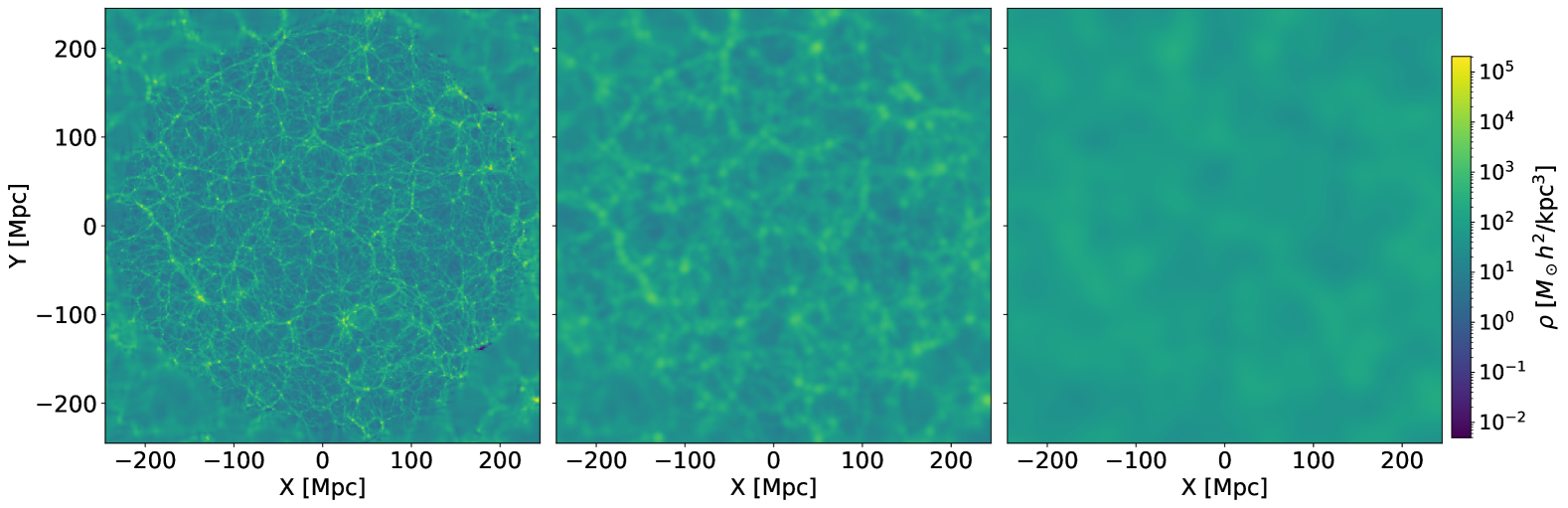
Figure 1: The dark matter distribution from a single realisation of CSiBORG, shown without and then with Gaussian smoothing of standard deviation $\sigma=2$ and $8$ Mpc/$h$ (middle and right panel). Each panel represents a 2D slice through the Z-axis of the simulation box, centred on the Milky Way. The high-completeness central region of radius 155 Mpc/$h$ is visible. As smoothing increases the smaller scale structures are smoothed out. See Section 2.1 for further details of CSiBORG, and Section 3.1 for further details of the smoothing methodology.

2.1 Simulation Data

Introduced in Bartlett et al. (2021), the CSiBORG suite comprises 101 $N$-body simulations. Spanning a three-dimensional box with dimensions of $677.7$ Mpc/$h$, centred on the Milky Way, these simulations use initial conditions inferred from the Bayesian Origin Reconstruction from Galaxies algorithm (BORG; Jasche & Wandelt 2013; Jasche et al. 2015; Leclercq 2015; Jasche & Lavaux 2019; Doeser et al. 2024; Stopyra et al. 2024) applied to the 2M++ galaxy survey (Lavaux & Hudson, 2011), which has a high completeness within a spherical region of radius $155$ Mpc/$h$ centred on the Milky Way. Specifically, this version of CSiBORG is based on the initial conditions presented in Jasche & Lavaux (2019).

The 2M++ reconstruction encompasses a cubic volume with a side length of $677.7$ Mpc/$h$ divided into $256^{3}$ voxels, resulting in a spatial resolution of $2.65$ Mpc/$h$. Similarly, CSiBORG features a high-resolution sphere centred on the Milky Way, with a radius of $155$ Mpc/$h$. In this region, initial conditions are augmented with white noise to account for random fluctuations on sub-constraint scales. The spatial distribution is defined on a grid measuring $2048^{3}$, yielding an initial inter-particle spacing of $0.33$ Mpc/$h$. Surrounding this high-resolution region, there is a spherical buffer zone with a width of $10$ Mpc/$h$, ensuring a smooth transition to the base BORG resolution. Figure 1 shows a slice of the CSiBORG box at different degrees of Gaussian smoothing (see Section 3.1). The three plots are zoomed in on the central region of high completeness. The left panel clearly shows a cross section of the central spherical high-completeness region.

Dark matter haloes are identified as in Stiskalek et al. (2024): within the central high-completeness region, the friends-of-friends halo finder (FOF; Davis et al. 1985) is used, with a linking-length parameter of $b=0.2$. The FOF algorithm connects particles within a distance $b$ times the mean particle separation. We require a minimum of 100 particles for a halo, corresponding to a minimum halo mass of $3.09\times 10^{11}M_{\odot}h^{-1}$.

The dark matter density field is reconstructed from $z=0$ particle snapshots. To convert them into a continuous density field, we employ the smoothed-particle hydrodynamics method (Monaghan, 1992; Colombi et al., 2007). As outlined in Section IV.B.1 of Bartlett et al. (2022), a minimum of 32 neighbouring particles is required to smooth over. The resulting density field is then mapped onto a grid with a resolution of $0.7~\mathrm{Mpc}/h$. Both BORG and CSiBORG adopt the following cosmological parameters: $T_{\rm{CMB}}=2.738$ K, $\Omega_{m}=0.307$, $\Omega_{\Lambda}=0.693$, $\Omega_{b}=0.04825$, $H_{0}=70.05$ km/s/Mpc, $\sigma_{8}=0.8288$ and $n=0.9611$. Lastly, for the purpose of this work we also use $20$ CSiBORG-like simulations but with random initial conditions to produce density fields that are uncorrelated with the observed galaxy properties.

2.2 Nasa-Sloan Atlas

We use the NSA survey to obtain galaxy properties such as the stellar mass ($M_{\star}$), colour ($u-r$), Sérsic index, size, and metallicity. A summary of these properties is provided in Table 1. However, it should be noted that the correlations with metallicity and stellar mass, presented in Section 4, should be used with caution, as stated explicitly in the NSA database.

The NSA database contains images and parameters of local galaxies, based on SDSS DR8 (Aihara et al., 2011) and the Galaxy Evolution Explorer survey (GALEX; Martin et al. 2005). We used the nsa_v1_0_1 data, which has a redshift range out to $z=0.15$ and contains $640\,000$ galaxies.

The distribution of these galaxies is illustrated in the right hand panel in Figure 2. After restricting the NSA sample to the region covered by 2M++, which was used to constrain the CSiBORG density field, we obtain a total of approximately $90\,000$ galaxies at a redshift of $z\leq 0.05$.

We obtain data for the star formation rate (SFR) and specific star formation rate (sSFR) of galaxies from MPA-JHU catalogue, which is based on Tremonti et al. (2004); Kauffmann et al. (2003); Brinchmann et al. (2004). This catalogue is part of data release 8 of the SDSS, and provides derived galaxy properties based on spectral measurements.

2.3 ALFALFA

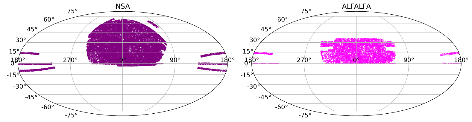
Figure 2: The distribution of NSA galaxies (left) and ALFALFA galaxies (right), shown on Mollweide projections of right ascension and declination. The NSA catalogue, based on optical data, contains information for 640,000 galaxies out to a redshift of 0.15. The ALFALFA catalogue provides $\mathrm{H}\scriptstyle\mathrm{I}$ 21 cm line measurements for 31,500 galaxies out to a redshift of 0.06, covering nearly 7000 deg² of high galactic latitude sky. See Section 2.2 and 2.3 for further information on the NSA and ALFALFA surveys respectively.

The ALFALFA survey maps nearly $7000~\rm{deg}^{2}$ of high galactic latitude sky using the Arecibo telescope, obtaining $\mathrm{H}\scriptstyle\mathrm{I}$ 21 cm line measurements for $31\,500$ galaxies out to a redshift of $0.06$  (Haynes et al., 2018). We use the ALFALFA galaxy $\mathrm{H}\scriptstyle\mathrm{I}$ masses.

We use an NSA and ALFALFA cross-match to obtain the $M_{\star}$, colour, SFR, Sérsic index, size and $\mathrm{H}\scriptstyle\mathrm{I}$ corresponding to ALFALFA galaxies. We match the NSA and ALFALFA catalogues by using a method following Stiskalek et al. (2021), exploiting the partial overlap between ALFALFA and SDSS. This method matches the optical counterpart position to the sources in the NSA using an on-sky angle tolerance and line-of-sight tolerance of 5 arcsec and 10 Mpc respectively. This constitutes a strict criteria ensuring a low likelihood of mismatches and high sample purity. This cross-match retains approximately $22\,000$ galaxies. There are some galaxies for which the density from CSiBORG is undefined (generally those galaxies outside of the high-completeness region - see Section 2.1). After removing these galaxies from our analysis, we retain approximately $8000$ galaxies in the ALFALFA dataset. Due to the flux-density limit of ALFALFA, there is a relatively steep Malmquist bias with redshift for the HI-detected galaxies. Furthermore, the galaxies in this ALFALFA-NSA dataset are bluer in colour than those from the general NSA galaxy sample, with higher star formation rates. The sky distribution of galaxies can be seen in the left hand plot of Figure 2.

3 Methodology

3.1 Density Statistics

We begin by defining statistics of the dark matter density field, which we then correlate with galaxy properties. We do this as follows. We conduct our analysis using 101 realisations of the CSiBORG simulations from which we obtain the dark matter density fields $\mathrm{\rho}\scriptstyle\mathrm{{}_{\rm DM}}$. For every realisation, we use the “native” SPH density field ($\rho_{0}$) along with four realisations of the field smoothed at different scales ($\rho_{d}$ for $d=2,\,4,\,8,\,16~\mathrm{Mpc}/h$). We choose these degrees of smoothing in order to provide insights across a large range of spatial scales. We then correlate these with the galaxy properties in Table 1. This allows us to investigate the effect of different spatial scales on various astrophysical processes. The Gaussian smoothing operates such that for a function $\rho(\mathbf{r})$, then

$$\rho_{\text{smoothed}}(\mathbf{r})=\dfrac{1}{\sigma^{3}(2\pi)^{\frac{3}{2}}}\int_{\mathcal{R}}\rho_{\text{\rm DM}}(\mathbf{r^{\prime}})\exp{\left({\dfrac{|\mathbf{r}-\mathbf{r^{\prime}}|^{2}}{2\sigma^{2}}}\right)}d\mathbf{r^{\prime}},$$ (1)

where $\sigma$ is the standard deviation of the Gaussian smoothing kernel in units of Mpc/$h$. The smoothed dark matter density field is rendered on a $1024^{3}$ grid such that the baseline of “no additional smoothing” has a spatial resolution of $0.66$ Mpc/$h$. This corresponds to the scale of a galaxy cluster (Bahcall, 1999). Note however that the constraints on the initial conditions are on a 2.6 Mpc/$h$ scale, and hence below this there is limited information on the actual density field. Figure 1 shows a 2D slice of a single CSiBORG realisation of the dark matter density field for $\rho_{0}$, $\rho_{2}$, and $\rho_{8}$. The effect of Gaussian smoothing can be seen on these plots, which show how finer features become more blurred as smoothing increases.

Estimating the dark matter density at the galaxy position should take into account its distance uncertainty. The NSA catalogue provides distances calculated using the Willick flow model (Willick et al., 1997), however no uncertainty is provided. The expected typical distance uncertainty due to small-scale velocities not accounted for by the model is $\sim 300$ km/s (Stiskalek et al., 2025), which corresponds to a distance uncertainty of $\sim 3$ Mpc/$h$. Therefore even our smallest smoothing scale should smooth out variations in the dark matter density comparably to the distance uncertainty (and the 2.6 Mpc/$h$ scale of the initial condition constraints).

3.2 Cosmic web statistics

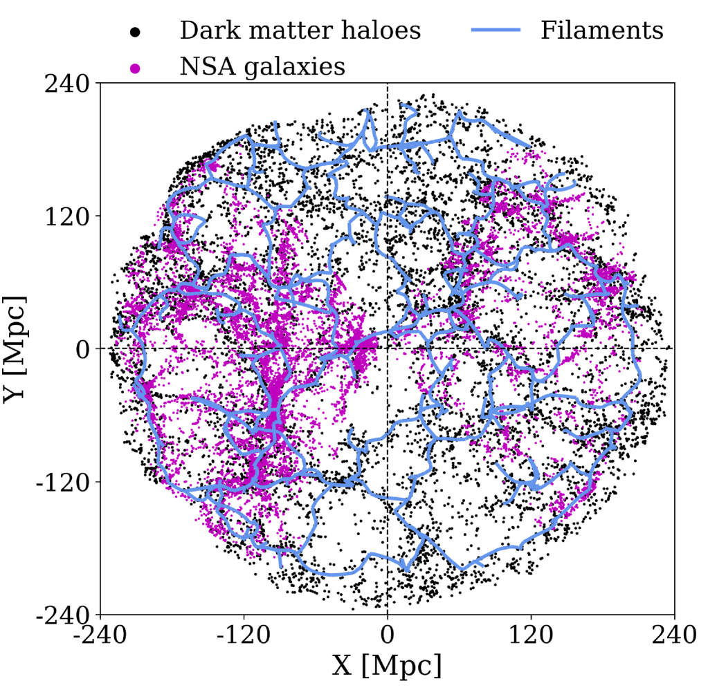
Figure 3: Distribution of dark matter haloes (black) derived from CSiBORG, overlaid with NSA galaxies (magenta), and cosmic web filaments (blue), shown in a 15 Mpc slice along the z-axis centred on the Milky Way. The cosmic web filaments are calculated using DisPerSE, applied to the CSiBORG haloes. NSA galaxies predominantly cluster along the filamentary structures, with some galaxies distributed within the voids of the cosmic web. See Section 2.1 for details on the CSiBORG haloes, and Section 3.2 for further details on the DisPerSE methodology and filament extraction.

To define the cosmic web we use the Discrete Persistence Structure Extractor algorithm (DisPerSE; Sousbie et al. 2011a, b). DisPerSE operates on particle data, which can be either observed galaxies or simulated dark matter haloes, and uses discrete Morse theory (Milner, 1963) to detect topological features: maxima, minima and saddle points. These features can then be used to convert the density field into the structural elements of the cosmic web: nodes, filaments, sheets, and voids. For our analysis, we apply DisPerSE to the 101 realisations of CSiBORG dark matter haloes, along with 20 unconstrained simulations to allow us to determine the statistical significance of our results (see Section 4).

The DisPerSE algorithm starts by constructing a 3-dimensional Delaunay tessellation field, using the Delaunay Tessellation Field Estimator (Schaap & van de Weygaert, 2000). We use periodic boundary conditions to estimate the particle density field. We then apply the “netconv” smoothing function to this density field, taking the smoothing threshold value as $1\sigma$. We then apply the “mse” function, which is the “manifold skeleton extractor” and the primary function of DisPerSE. This identifies the critical points of the density field and requires the user to input a persistence threshold, which we take to be 2$\sigma$. This threshold is important as if it is too low, it may lead DisPerSE to map noise as filaments, or if too high, DisPerSE may miss the finer structures.

The values that we take for smoothing and persistence threshold are consistent with Galárraga-Espinosa et al. (2024), who look for the the optimal smoothing and persistence threshold parameters that recover the most accurate cosmic web features while minimising noise. We then apply the “skelconv” function to convert the outputs into a readable format, with critical points indicating when the gradients of the manifold are equal to zero. The critical points are maxima, minima and saddle points. The filament arms are given by connecting a maxima to a saddle point and are made up of many small segments. The filament distribution overlaid on one realisation of the dark matter haloes, alongside the observational data is shown in Figure 3.

With the filament locations identified, we calculate the midpoint of each segment, and compare these with the galaxy coordinates from the NSA database, in order to compile a list of the “distance to the nearest filament” for every galaxy, which we hereafter refer to as $\mathrm{d}\scriptstyle\mathrm{{}_{fil}}$. As the average segment size is about 1 Mpc, the error from the discretisation of the filament is negligible. The process produces 101 separate sets of $\mathrm{d}\scriptstyle\mathrm{{}_{fil}}$, each corresponding to a realisation of the CSiBORG dark matter haloes. Additionally we obtain 20 sets of $\mathrm{d}\scriptstyle\mathrm{{}_{fil}}$ corresponding to the unconstrained simulations.

3.3 Correlation Statistics

We use two methods to calculate the correlation between data sets: a direct Spearman correlation between two properties (“direct correlation”), and a partial Spearman correlation conditioned on $M_{\star}$, $\mathrm{\rho}\scriptstyle\mathrm{{}_{\rm DM}}$, or $\mathrm{d}\scriptstyle\mathrm{{}_{fil}}$ (“partial correlation”).

The Spearman rank correlation coefficient quantifies whether a relation between two variables can be described by a monotonic function. Unlike the Pearson correlation coefficient, which measures linear relationships, the Spearman correlation coefficient takes into account the ranks of the data points rather than their raw values. Therefore, it is less sensitive to outliers, since outliers have a smaller effect on the ranking of the data. The Spearman correlation coefficient is calculated by considering $n$ pairs of observations from two distributions, with the observations in each distribution ranked from smallest to largest (Kendall & Stuart, 1973). Then, if $d_{i}$ is the difference between the ranks of each observation, the Spearman rank correlation coefficient, $r_{S}$, is given by

$$r_{S}=1-\dfrac{6\sum d_{i}^{2}}{n(n^{2}-1)}.$$ (2)

We also use a partial correlation method to quantify the relationship between a galaxy property and either $\mathrm{\rho}\scriptstyle\mathrm{{}_{\rm DM}}$ or $\mathrm{d}\scriptstyle\mathrm{{}_{fil}}$, while controlling for a third property: $M_{\star}$, $\mathrm{\rho}\scriptstyle\mathrm{{}_{\rm DM}}$ or $\mathrm{d}\scriptstyle\mathrm{{}_{fil}}$. This is achieved by fitting a locally weighted scatter plot function (LOWESS; Cleveland 1979) between each variable of interest ($A$ and $B$) and the third property ($C$, the condition). LOWESS fits a generalised non-linear function to the data, by locally fitting a weighted least squares regression line. We use LOWESS as it handles outliers more reliably than a basic curve fit function, and allows for flexibility in the fit when handling complex data with a non-trivial relationship. We then compute the residuals from the fit between A and C and then between B and C. The Spearman rank correlation coefficient is calculated between the two sets of residuals, providing the partial correlation between A and B, conditioned on property $C$.

Where there is a bimodal relationship between a variable and stellar mass, we separate the two distributions. For example, with colour, SFR, and sSFR we separate “quenched” and “star forming” galaxies in line with the process later described in Section 3.4 and visible in Figure 5. We find the residuals of these distributions separately. Figure 4 shows how the residuals were found for colour, after splitting the bimodal colour distribution as star forming or quenched galaxies.

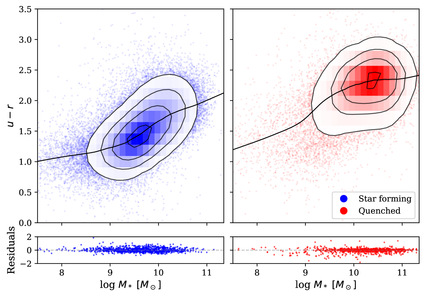
Figure 4: The relationship between colour ($u-r$) and stellar mass, with the solid black line showing the LOWESS fit. The bimodal distribution of colour has been separated into “star forming” (left) and “quenched” (right). The contour lines show the points contained within $0.5\sigma$, $1\sigma$, $1.5\sigma$, and $2\sigma$, which represents 11.8$\%$, 39.3$\%$, 67.5$\%$ and 86.4$\%$ regions of each distribution, respectively.

We apply the above procedure to extract the correlation coefficients between galaxy and environmental properties ($\mathrm{\rho}\scriptstyle\mathrm{{}_{\rm DM}}$ and $\mathrm{d}\scriptstyle\mathrm{{}_{fil}}$) for the 101 constrained simulations as well as the 20 unconstrained simulations. We find that for the unconstrained simulations, the distributions of correlation coefficients are approximately Gaussian and centred on zero. We find that the standard deviations of the distributions are much smaller for the constrained simulations than the unconstrained simulations, showing the uncertainty due to the BORG posterior is small. We perform bootstrapping with replacement to test the uncertainty due to the finite sample size of the galaxy surveys, but find it is negligible.

Given the above, we quantify the statistical significance of each correlation as the mean of the correlation coefficients from the constrained simulations divided by the standard deviation of the coefficients from the unconstrained simulations. This tests against the null hypothesis of no correlation between environment and any of the galaxy properties, which is necessarily the case in the unconstrained simulations.

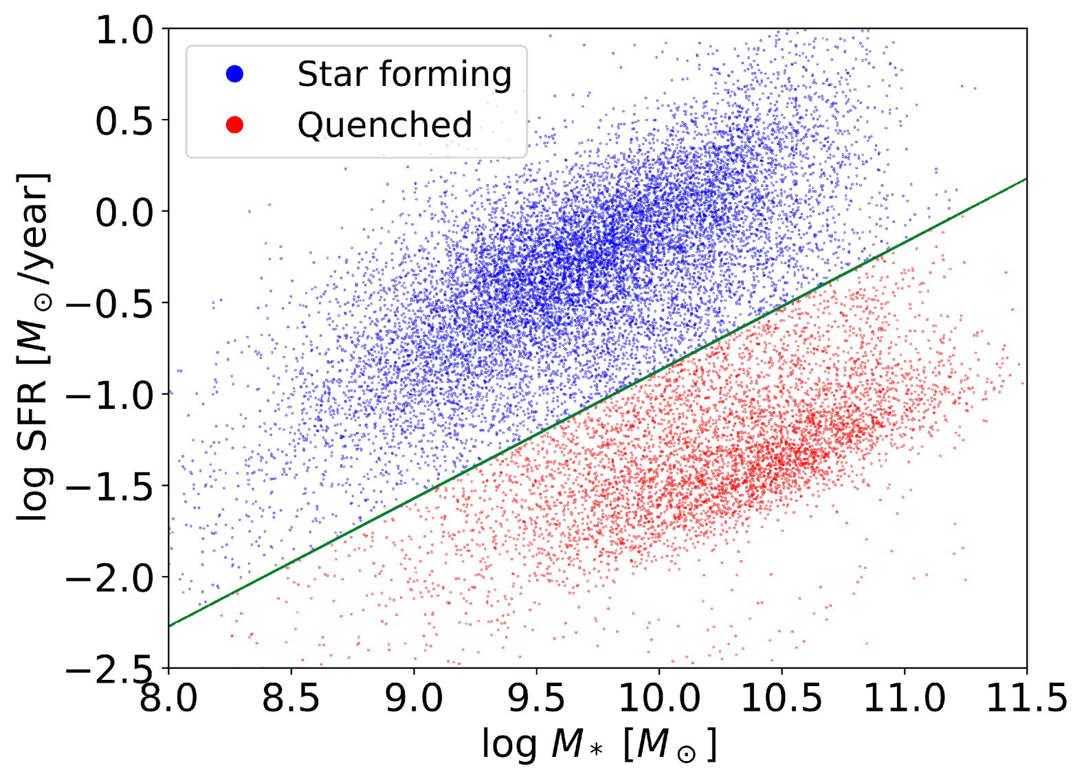
Figure 5: The bimodal distribution of the star formation rate of NSA galaxies (from the MPA/JHU catalogue), classifying galaxies as star forming (blue; above the dividing line) and quenched (red; below the dividing line). We use Equation 3 to divide the two populations. See Section 3.4 for further details on the methodology of defining a quenched galaxy.

3.4 Quenched Fraction

We also want to study the dependence of the quenched fraction of galaxies on $\mathrm{\rho}\scriptstyle\mathrm{{}_{\rm DM}}$ and $\mathrm{d}\scriptstyle\mathrm{{}_{fil}}$. In Figure 5 we plot the star formation rate (from the MPA/JHU catalogue) against $M_{\star}$, which produces a bimodal distribution of galaxies. This can be split into galaxies on the “main sequence,” which we define as star forming, and those below this main sequence band, which we define as quenched.

We define galaxies as star forming or quenched with the following definition of the main sequence from Whitaker et al. (2012):

$$\log_{10}(\text{SFR/M}_{\odot}~\text{yr}^{-1})=\alpha(z)[\log_{10}(M_{\star}/\text{M}_{\odot})-10.5]+\beta(z),$$ (3)

where the slope $\alpha(z)=0.70-0.13z$ and the normalisation factor $\beta(z)=0.38+1.14z-0.19z^{2}$. We then subtract 1 dex from $\log_{10}(\text{SFR})$ in order to find the line separating the star forming and quenched sequences, as this is approximately at the minima between the star formation main sequence and the population of quenched galaxies.

4 Results

Here we present the results obtained for the relationship of galaxy properties (described in Table 1) with environmental density $\mathrm{\rho}\scriptstyle\mathrm{{}_{\rm DM}}$ and distance from filament $\mathrm{d}\scriptstyle\mathrm{{}_{fil}}$. For simplicity, we will henceforth refer to the ALFALFA$\times$NSA data as “ALFALFA data”.

In Figure 6 we show the relationship between dark matter density and distance from filament (inferred from CSiBORG) evaluated at the position of NSA galaxies. As expected, there is a strong anti-correlation between mean density and distance to filament. To fully investigate the relative effect of filament distance and density on galaxy properties, we study their correlations with $\mathrm{\rho}\scriptstyle\mathrm{{}_{\rm DM}}$ and $\mathrm{d}\scriptstyle\mathrm{{}_{fil}}$ individually, as well as their correlation with $\mathrm{\rho}\scriptstyle\mathrm{{}_{\rm DM}}$ conditioned on $\mathrm{d}\scriptstyle\mathrm{{}_{fil}}$ and vice-versa.

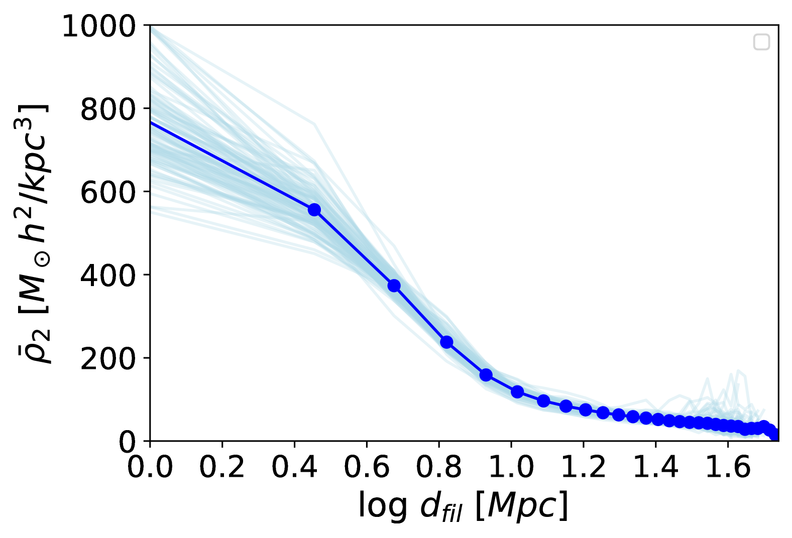
Figure 6: The relationship between the matter density $\rho_{2}$ and distance to nearest filament $\mathrm{d}\scriptstyle\mathrm{{}_{fil}}$ evaluated at the position of NSA galaxies. The thin lines are the relations inferred from individual CSiBORG realisations, whereas the bold blue is their mean. $\rho_{2}$ rapidly decreases with $\mathrm{d}\scriptstyle\mathrm{{}_{fil}}$, affirming that the dark matter density is concentrated around the filament, and that there is a sharp density gradient surrounding the filament.

4.1 NSA Correlations

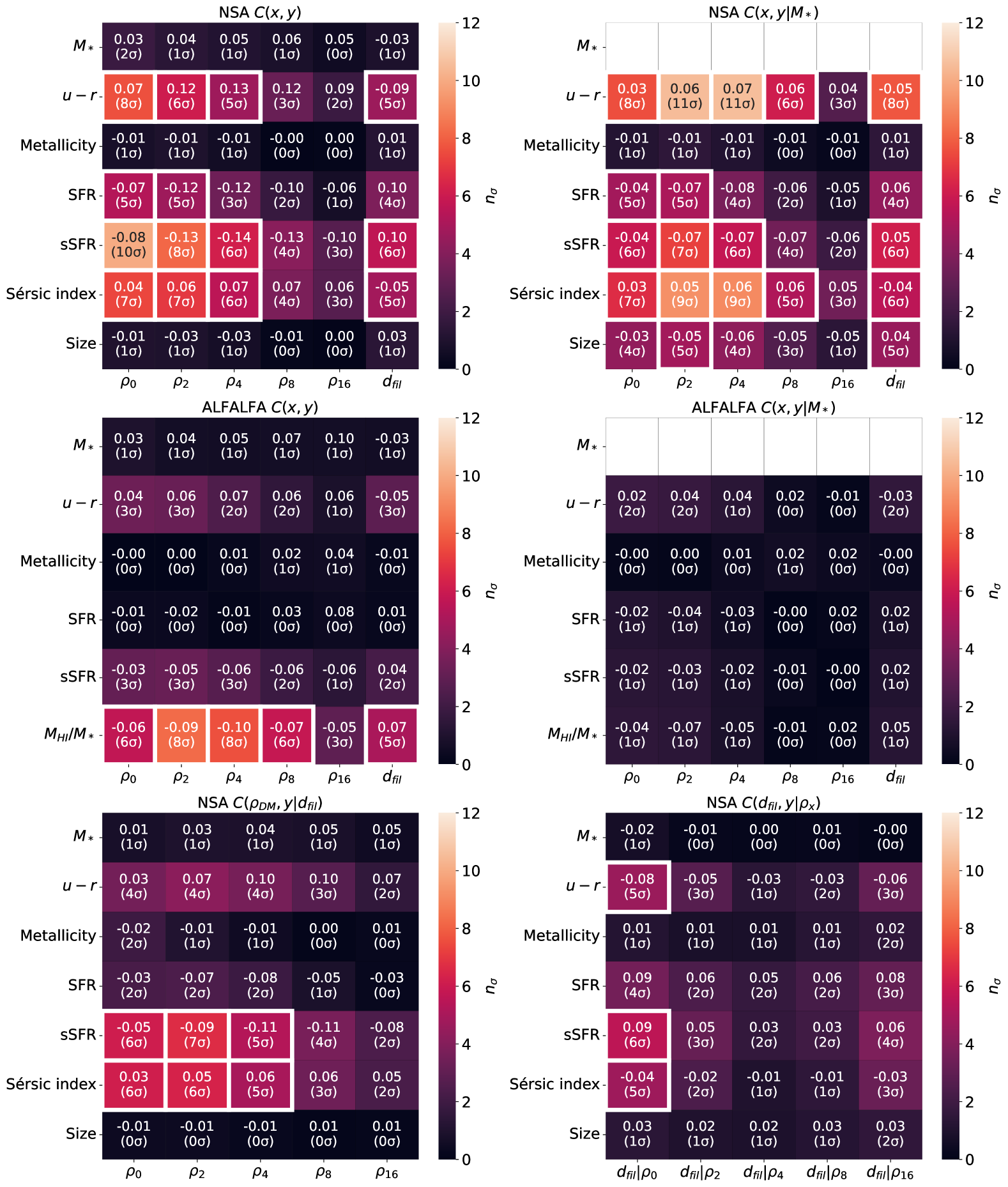
Figure 7: Correlation coefficients of galaxy properties with $\mathrm{\rho}\scriptstyle\mathrm{{}_{\rm DM}}$ and $\mathrm{d}\scriptstyle\mathrm{{}_{fil}}$, with a white box indicating correlations of at least $5\sigma$ statistical significance. The first row shows the direct correlation (left) and partial correlation conditioned on $M_{\star}$ (right) between NSA galaxy properties and $\mathrm{\rho}\scriptstyle\mathrm{{}_{\rm DM}}$ or $\mathrm{d}\scriptstyle\mathrm{{}_{fil}}$. The second row shows the same correlations for ALFALFA galaxies. The third row shows the partial correlation between NSA galaxy properties and $\mathrm{\rho}\scriptstyle\mathrm{{}_{\rm DM}}$ conditioned on $\mathrm{d}\scriptstyle\mathrm{{}_{fil}}$ (left), and the partial correlation between NSA galaxy properties and $\mathrm{d}\scriptstyle\mathrm{{}_{fil}}$ conditioned on $\mathrm{\rho}\scriptstyle\mathrm{{}_{\rm DM}}$ (right). Correlations of galaxy properties with the dark matter density are typically stronger than those with the filament distance. See Section 4 and Section 5.1 for a description and interpretation of these results respectively.

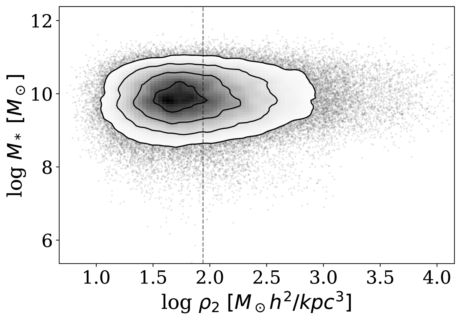
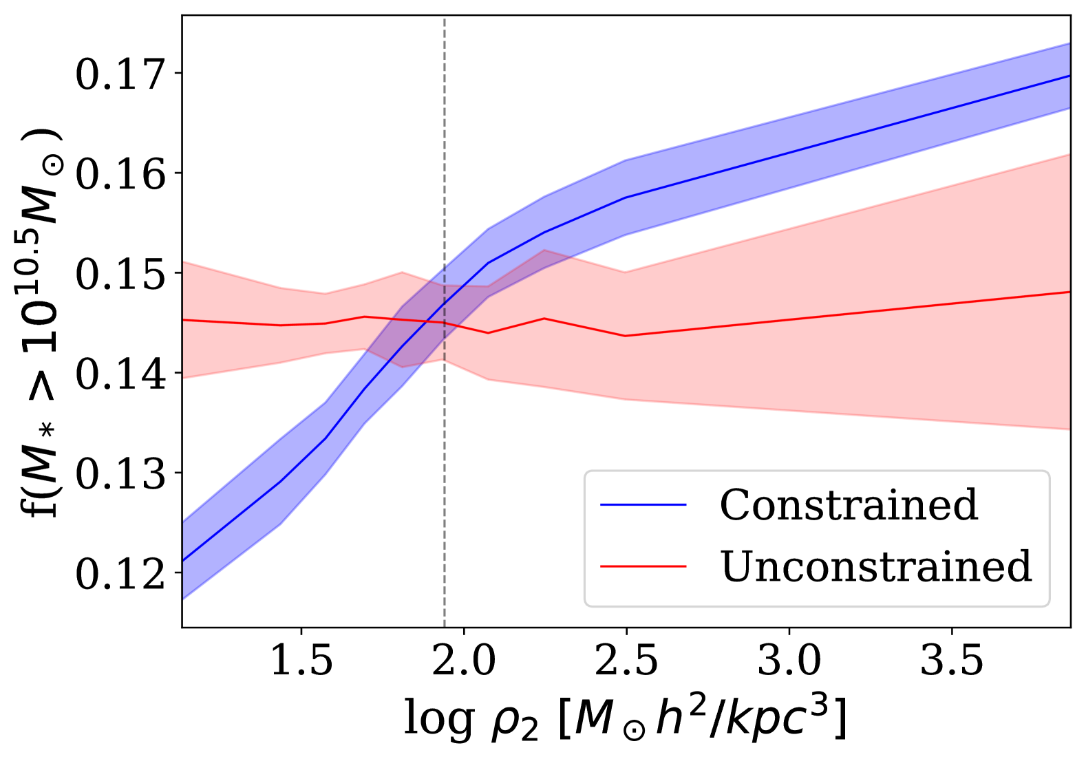
Figure 8: The relationship between dark matter density $\rho_{2}$ and stellar mass $M_{\star}$ (left) and the fraction of high mass galaxies ($M_{\star}>10^{10.5}M_{\odot}$) in bins of $\rho_{2}$ (right). The dashed vertical line on each plot shows the average matter density. The contour lines on the left panel are at $0.5\sigma$, $1\sigma$, $1.5\sigma$, and $2\sigma$, containing 11.8$\%$, 39.3$\%$, 67.5$\%$ and 86.4$\%$ of the points, respectively. The solid lines on the right panel show the mean fraction of high mass galaxies in density bins across 101 constrained (blue) simulations and 20 unconstrained (red) simulations, with the shaded regions representing the standard deviation across the respective set of simulations. The constrained simulations show a positive correlation between fraction of high mass galaxies and density, while the unconstrained simulations show no correlation and a very high standard deviation towards high densities.

The results for the Spearman correlations of galaxy properties taken from the NSA survey (see Table 1) with $\mathrm{\rho}\scriptstyle\mathrm{{}_{\rm DM}}$ and $\mathrm{d}\scriptstyle\mathrm{{}_{fil}}$ are shown in the top and bottom rows of Figure 7. This figure shows the direct correlation between galaxy properties with $\mathrm{\rho}\scriptstyle\mathrm{{}_{\rm DM}}$ and $\mathrm{d}\scriptstyle\mathrm{{}_{fil}}$ in the top left panel, the partial correlation conditioned on $M_{\star}$ between galaxy properties with $\mathrm{\rho}\scriptstyle\mathrm{{}_{\rm DM}}$ and $\mathrm{d}\scriptstyle\mathrm{{}_{fil}}$ in the top right panel, the partial correlation between galaxy properties and $\mathrm{\rho}\scriptstyle\mathrm{{}_{\rm DM}}$ conditioned on $\mathrm{d}\scriptstyle\mathrm{{}_{fil}}$ in the bottom left panel, and the partial correlation with $\mathrm{d}\scriptstyle\mathrm{{}_{fil}}$ conditioned on $\mathrm{\rho}\scriptstyle\mathrm{{}_{\rm DM}}$ in the bottom right panel. We show the statistical significance of each correlation in parentheses below the value of the correlation, with a description of how this was calculated in Section 3.3.

The direct correlations of both $\mathrm{\rho}\scriptstyle\mathrm{{}_{\rm DM}}$ and $\mathrm{d}\scriptstyle\mathrm{{}_{fil}}$ with galaxy properties (colour, SFR, sSFR and Sérsic index) are statistically significant. For $\mathrm{\rho}\scriptstyle\mathrm{{}_{\rm DM}}$, the correlation peaks around $\rho_{0}$ or $\rho_{2}$, generally showing stronger correlations than those for $\mathrm{d}\scriptstyle\mathrm{{}_{fil}}$, with comparable or higher statistical significance (e.g. correlation coefficient of -0.13 with statistical significance $8\sigma$ for $\rho_{2}$ with sSFR, compared to 0.10 and statistical significance $6\sigma$ for $\mathrm{d}\scriptstyle\mathrm{{}_{fil}}$). When conditioned on stellar mass, size displays stronger correlations with $\mathrm{\rho}\scriptstyle\mathrm{{}_{\rm DM}}$ than the direct correlation. Notably, conditioning on $\mathrm{d}\scriptstyle\mathrm{{}_{fil}}$ yields stronger correlations than conditioning on $\mathrm{\rho}\scriptstyle\mathrm{{}_{\rm DM}}$.

There is a notably weak correlation between $M_{\star}$ and $\mathrm{\rho}\scriptstyle\mathrm{{}_{\rm DM}}$ with a low statistical significance. This is surprising as previous studies have shown that high mass galaxies have a high correlation with environmental density (e.g. Yoon et al. 2017). We tested this by defining a set of high mass galaxies ($M_{\star}>10^{10.5}M_{\odot}$) and find the fraction of high mass galaxies in bins of $\mathrm{\rho}\scriptstyle\mathrm{{}_{\rm DM}}$. The right panel of Figure 8 shows this fraction as a function of density: there is a (weak) positive correlation, affirming that high mass galaxies tend to be found in denser environments. It is likely that the more scattered distribution of low mass galaxies washes out the correlation between $M_{\star}$ and $\mathrm{\rho}\scriptstyle\mathrm{{}_{\rm DM}}$, hence why we see a very low correlation between $M_{\star}$ and $\mathrm{\rho}\scriptstyle\mathrm{{}_{\rm DM}}$ in Figure 7.

4.2 ALFALFA correlations

Next we investigate the correlation between $\mathrm{\rho}\scriptstyle\mathrm{{}_{\rm DM}}$ and $\mathrm{d}\scriptstyle\mathrm{{}_{fil}}$ with galaxy properties for the ALFALFA galaxies. In addition to the galaxy properties investigated for the NSA data, we also include the $M_{\mathrm{H}\scriptstyle\mathrm{I}}/M_{\star}$ . The correlation results are presented in the middle row of Figure 7, with the direct correlation in the left panel, and the partial correlation conditioned on $M_{\star}$ in the right panel.

The direct correlation for the ALFALFA data reveals statistically significant negative correlations between $M_{\mathrm{H}\scriptstyle\mathrm{I}}/M_{\star}$ and $\mathrm{\rho}\scriptstyle\mathrm{{}_{\rm DM}}$, with the strongest correlation and peak statistical significance with $\rho_{4}$. The ALFALFA partial correlation conditioned on $M_{\star}$ reveals very weak correlations of low statistical significance across all galaxy properties. The highest statistical significance is $2\sigma$ for the correlations with colour. The ALFALFA partial correlations conditioned on $M_{\star}$ between any property and $\mathrm{d}\scriptstyle\mathrm{{}_{fil}}$ are weak and of low statistical significance.

The weak correlations displayed by the ALFALFA galaxy properties are likely due to the selection effects of the ALFALFA survey, which contains preferentially bluer, star forming galaxies, as these tend to be $\mathrm{H}\scriptstyle\mathrm{I}$ rich. This selection results in a narrower range of galaxy properties, reducing the observed correlation strengths. Additionally, the smaller sample size of the ALFALFA dataset likely contributes to the weak correlations and low statistical significance.

4.3 Galaxy quenching

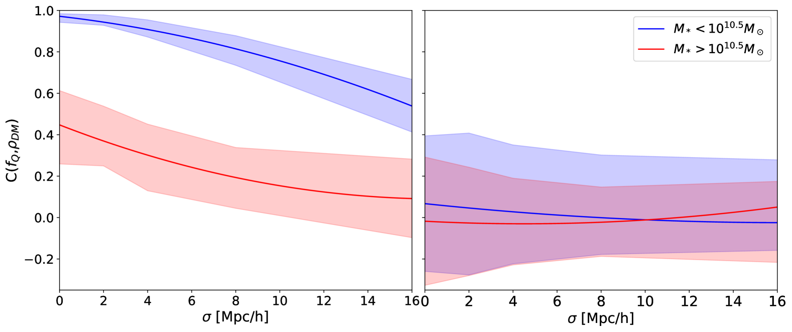
Figure 9: The mean correlation between the fraction of quenched galaxies $f_{Q}$ and the environmental density $\mathrm{\rho}\scriptstyle\mathrm{{}_{\rm DM}}$ from constrained simulations (left) and unconstrained simulations (right) as a function of the Gaussian smoothing scale, $\sigma$. The solid lines and shading show the mean and $1\sigma$ uncertainty across the CSiBORG realisations, respectively. We separately show low mass (blue, $M_{\star}<10^{10.5}M_{\odot}$) and high mass (red, $M_{\star}>10^{10.5}M_{\odot}$) galaxies. Low mass galaxies exhibit a much stronger correlation with environment than high mass galaxies, suggesting that quenching in low mass galaxies is primarily driven by external mechanisms, while in high mass galaxies, internal mechanisms play a larger role. See Section 4.3 and Section 5.1.2 for further description and analysis of these results.

We now investigate the relationship between the dark matter density, distance to nearest filament and the quenching of galaxies in the NSA catalogue. We test this separately for low and high mass galaxies, as previous studies suggest that quenching mechanisms can depend on galaxy mass (Bluck et al., 2014; Goubert et al., 2024; Zheng et al., 2025). Following Goubert et al. (2024), we define a high mass galaxy as $M_{\star}>10^{10.5}M_{\odot}$.

Figure 9 shows the correlation between $\mathrm{\rho}\scriptstyle\mathrm{{}_{\rm DM}}$ and the fraction of quenched galaxies across different smoothing scales. The solid lines represent the average correlation (mean of 101 realisations of CSiBORG) as a function of smoothing scale for high mass (red) and low mass (blue) galaxies. The shaded area shows the standard deviation across the 101 realisations.

The correlation between the fraction of quenched galaxies and $\mathrm{\rho}\scriptstyle\mathrm{{}_{\rm DM}}$ is stronger for low mass galaxies than for high mass galaxies. For both high and low mass galaxies, the correlation decreases while smoothing scale increases. The standard deviation increases towards $\rho_{16}$ (particularly for the low mass galaxies), likely due to the fact that the result becomes increasingly randomised as the scale becomes less relevant. Following the split, we have $\sim$ 76,000 and $\sim$ 13,000 low- and high-mass galaxies, respectively, thus the standard deviation in the correlation coefficient of high-mass galaxies is larger.

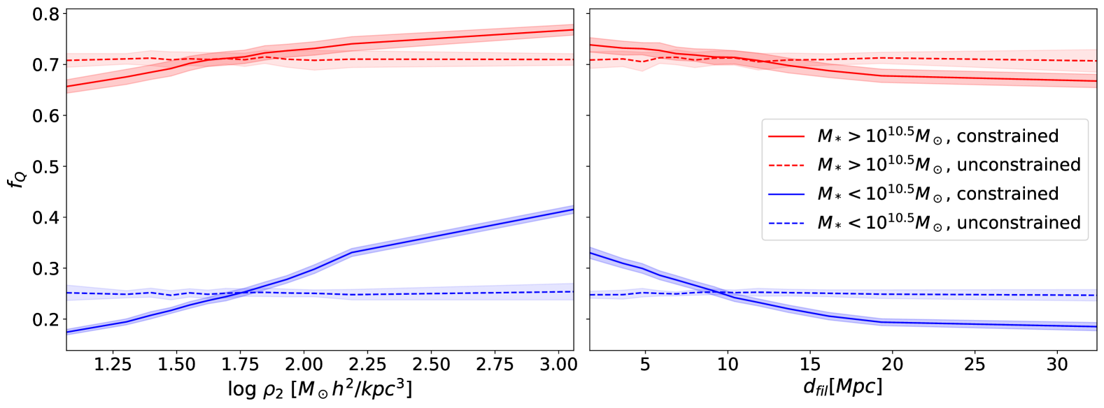
Figure 10: The fraction of quenched galaxies $f_{Q}$ across bins of $\rho_{2}$ (left) and bins of $\mathrm{d}\scriptstyle\mathrm{{}_{fil}}$ (right) for low mass (blue, $M_{\star}<10^{10.5}M_{\odot}$) and high mass (red, $M_{\star}>10^{10.5}M_{\odot}$) galaxies. The solid lines and shading show the mean correlation and its $1\sigma$ uncertainty, respectively, for constrained simulations. The dotted lines and shading show the equivalent for unconstrained simulations. $f_{Q}$ increases as $\rho_{2}$ increases, suggesting that greater environmental densities are associated with higher quenching rates. $f_{Q}$ decreases as $\mathrm{d}\scriptstyle\mathrm{{}_{fil}}$ increases, indicating that galaxies further from filaments are less likely to experience quenching. $f_{Q}$ begins to flatten at around $d_{\rm fil}=15~\mathrm{Mpc}$, while $f_{Q}$ increases for each value of $\rho_{2}$. When compared to unconstrained simulations, the plots show that the relationship between $f_{Q}$ and environment is far stronger for low mass galaxies than for high mass galaxies. See Section 5.1.2 for further interpretation of these results.

Lastly, Figure 10 shows how the fraction of quenched galaxies changes with $\mathrm{d}\scriptstyle\mathrm{{}_{fil}}$ and $\rho_{2}$. We choose $\rho_{2}$ for this analysis, as this scale produces the greatest statistical significance for the majority of the correlations in Figure 7. We see a stronger correlation between environment and quenched fraction for low mass galaxies than high mass galaxies, in line with Figure 9. We also see that while quenched fraction continues to increase with $\rho_{2}$, it begins to flatten at around 15 Mpc for $\mathrm{d}\scriptstyle\mathrm{{}_{fil}}$.

5 Discussion

5.1 Interpretation of results

An advantage of CSiBORG is that the multiple realisations correspond to the uncertainty with which we know the density field. By comparing the correlation strength of each realisation of the constrained simulations we can see this uncertainty is subdominant. This implies a low uncertainty due to the BORG posterior. Additionally, bootstrapping galaxies within the sample shows that the uncertainty due to sample size is minimal. The dominant source of uncertainty arises from comparing the correlation from constrained simulations to that from unconstrained simulations, a process described in Section 3.3.

5.1.1 Star formation and $\mathrm{H}\scriptstyle\mathrm{I}$ content

We now consider the implications of the SFR and $M_{\mathrm{H}\scriptstyle\mathrm{I}}/M_{\star}$ correlations on models of galaxy formation. Both the NSA and ALFALFA correlation results imply that as $\mathrm{\rho}\scriptstyle\mathrm{{}_{\rm DM}}$ increases, a galaxy is less likely to be star forming, will have a lower $M_{\mathrm{H}\scriptstyle\mathrm{I}}/M_{\star}$, and will be redder in colour. In the literature these trends are often attributed to effects such as “gas heating” (where the intergalactic medium around galaxies is heated by external sources like shocks or AGN feedback, preventing gas from cooling or forming stars, e.g. McNamara & Nulsen 2007), “strangulation” (the cessation of cold gas inflow onto a galaxy, e.g. Kawata & Mulchaey 2008), or the effect of “galaxy group interactions” near filaments (for example ram pressure stripping, mergers, and tidal forces between galaxies which often lead to tidal stripping, e.g. Gunn & Gott 1972; Roediger & Hensler 2005; McCarthy et al. 2008).

Consistent with the correlations for $\mathrm{\rho}\scriptstyle\mathrm{{}_{\rm DM}}$, the results for $\mathrm{d}\scriptstyle\mathrm{{}_{fil}}$ imply that galaxies closer to filaments have a lower $M_{\mathrm{H}\scriptstyle\mathrm{I}}/M_{\star}$ and are redder in colour. While of reasonable statistical significance, the direct correlation coefficients are weak. The partial correlations conditioned on $M_{\star}$ are of negligible statistical significance. Together these results suggest that gas feeding galaxies from filaments is not strongly prevalent in the local Universe. Our results are qualitatively consistent with Kraljic et al. (2018), who find that at lower redshift, filaments are not expected to boost gas flow and therefore increase the quantity of gas or star formation rate in galaxies. However at high redshifts, the role of the cosmic web is expected to be more important, with gas flow from filaments into galaxies an important effect, as shown by Ramsøy et al. (2021).

5.1.2 Quenching

The results presented on the relationship between fraction of quenched galaxies and $\mathrm{\rho}\scriptstyle\mathrm{{}_{\rm DM}}$ align with Goubert et al. (2024), who argue that low mass galaxies experience quenching predominantly due to their environment. Goubert et al. (2024) link quenching in low mass galaxies to properties such as host halo mass and galaxy overdensity. On the other hand, they find that quenching in high mass galaxies is likely to be due to internal processes such as AGN feedback. Our results support this idea, showing that the quenching of high mass galaxies has a low dependence on environment. This is evident in Figure 9, where the correlation between $\mathrm{\rho}\scriptstyle\mathrm{{}_{\rm DM}}$ and quenched fraction is far weaker for high mass galaxies than low mass galaxies. Porqueres et al. (2018) find the relationship between AGN properties and environmental density inferred from BORG is more important than the cosmic web structure. However, an alternative possibility is that the most quenched galaxies are simply the oldest ones, residing in the oldest and most dense haloes, meaning that the observed trend does not necessarily imply AGN-driven quenching. Further confirmation from simulations would be needed to confirm the cause of this quenching.

Figure 9 shows that the correlation between the fraction of quenched galaxies and $\mathrm{\rho}\scriptstyle\mathrm{{}_{\rm DM}}$ decreases as the degree of smoothing increases. This suggests that the mechanisms driving the quenching of galaxies operate on smaller spatial scales. While the voxel resolution of $\rho_{0}$ is $0.7~\mathrm{Mpc}/h$, which roughly corresponds to the scale of a galaxy cluster, the BORG initial conditions are constrained with a voxel resolution four times larger. This could imply that the quenching of low mass galaxies, with their strong positive correlation at $\rho_{0}$, is directly related to the internal processes on the scale of galaxy clusters. This would be consistent with the correlations discussed in Section 5.1.1: galaxies in higher density environments have lower $\mathrm{H}\scriptstyle\mathrm{I}$ mass content and star formation rates, likely due to the processes such as gas heating, strangulation and the effects of galaxy group environments. The strongest correlation between $\mathrm{\rho}\scriptstyle\mathrm{{}_{\rm DM}}$ and quenched fraction is $\rho_{0}$ supporting the idea that the internal processes of a galaxy cluster play a very important role in the quenching of a galaxy.

Figure 10 shows similar trends between the quenched fraction of galaxies in bins of $\rho_{2}$ and in bins of $\mathrm{d}\scriptstyle\mathrm{{}_{fil}}$. Both show weaker correlations between environment and high mass galaxies, as expected, and both show steep correlations between low mass galaxies and environment. The most notable difference between the two, is that the relationship between low mass galaxies and $\mathrm{d}\scriptstyle\mathrm{{}_{fil}}$ begins to flatten at around 15 Mpc from the filament. In comparison, the trend with $\rho_{2}$ continues to increase with density. This suggests that after a certain distance from filament, the environmental processes linked to quenching are no longer effective. This can be explained by the relationship between $\mathrm{d}\scriptstyle\mathrm{{}_{fil}}$ and $\mathrm{\rho}\scriptstyle\mathrm{{}_{\rm DM}}$, which we show in Figure 6. There is a steep density gradient close to filaments that begins to flatten at around 15 Mpc from the filament and continues to do so up to 40 Mpc from the filament. Wang et al. (2024) find that the maximum density gradient is at 1 Mpc from the filament centre, which suggests that this is where we could expect to see the biggest impact of ram pressure stripping at least. This could suggest that $\mathrm{\rho}\scriptstyle\mathrm{{}_{\rm DM}}$ is the dominant factor in the environmental quenching of galaxies, as it is the density gradient associated with a filament that is causing quenching, rather than the mechanisms associated with the filamentary structure itself.

5.1.3 Morphology and size

We take the Sérsic index as analogous to the morphology of a galaxy where a Sérsic index of $\lesssim 1.5$ approximately corresponds to disk galaxies, whereas a Sérsic index of $\gtrsim 3$ corresponds to elliptical galaxies. Therefore, our results for NSA correlations suggest that as density increases, the fraction of elliptical galaxies increases. This is in agreement with the theory that elliptical galaxies often form in a “hierarchical” formation scenario through mergers between galaxies (De Lucia et al., 2006). Mergers are more likely in high density environments due to the increased frequency of close galaxy encounters (see e.g. Pearson et al. 2024). The correlation of the Sérsic index with $\mathrm{d}\scriptstyle\mathrm{{}_{fil}}$ supports this idea, suggesting that the closer a galaxy is to a filament, the more likely it is to be elliptical. However, this correlation is weaker than those with $\mathrm{\rho}\scriptstyle\mathrm{{}_{\rm DM}}$, suggesting that $\mathrm{\rho}\scriptstyle\mathrm{{}_{\rm DM}}$ is the dominant factor in influencing the morphology of a galaxy.

The correlation coefficients we find could imply that galaxies of a smaller radius are generally located in higher density areas, particularly when controlling for $M_{\star}$. However the statistical significance of the correlations for size is low, rendering our results as inconclusive; there is no significant correlation between size and $\mathrm{\rho}\scriptstyle\mathrm{{}_{\rm DM}}$ or $\mathrm{d}\scriptstyle\mathrm{{}_{fil}}$. Nevertheless, this is an interesting result considering conflicting conclusions in the literature. Ghosh et al. (2024) investigate the relationship between galaxy size and environment at higher redshifts ($z\geq 0.3$), reporting that larger galaxies are more likely to be found in higher density environments, independent of galaxy morphology or stellar mass. This is consistent with Mercado et al. (2025), who find that low mass galaxies ($M_{\star}<10^{9}M_{\odot}$) are larger if they are experiencing stronger tidal influences (consistent with a higher density environment). This however contrasts with our findings at a lower redshift. Ghosh et al. (2024) provide a useful analysis of the conflicting galaxy size-environment results throughout the literature. They argue that size is dependent on morphology and $M_{\star}$, meaning that these factors should be controlled in order to understand the correlation with environment. This could explain the low strength and statistical significance for the correlation between size and environment.

Other studies focusing on the local Universe also show conflicting results. Huertas-Company et al. (2013) find that early type galaxies show no correlation between their mass-size relation and environment, while Shankar et al. (2013) find that spheroids in more massive host haloes, where a spheroid is defined as an elliptical galaxy or a galaxy with a large central bulge, have a larger size at fixed $M_{\star}$. It is worth noting that these studies rely on observations or semi-analytical models, whereas our analysis uses constrained N-body simulations, which could account for some differences.

5.1.4 The relative importance of $\mathrm{\rho}\scriptstyle\mathrm{{}_{\rm DM}}$, $\mathrm{d}\scriptstyle\mathrm{{}_{fil}}$, and $\sigma$

Throughout the results and discussion, we compare the correlations found for galaxy properties with $\mathrm{\rho}\scriptstyle\mathrm{{}_{\rm DM}}$ to those found for galaxy properties with $\mathrm{d}\scriptstyle\mathrm{{}_{fil}}$. We find consistently stronger and more statistically significant correlations with $\mathrm{\rho}\scriptstyle\mathrm{{}_{\rm DM}}$ than with $\mathrm{d}\scriptstyle\mathrm{{}_{fil}}$. Additionally, the middle row in Figure 7, shows that controlling for $\mathrm{d}\scriptstyle\mathrm{{}_{fil}}$, gives stronger and more statistically significant correlations than controlling for $\mathrm{\rho}\scriptstyle\mathrm{{}_{\rm DM}}$, suggesting that the effects of $\mathrm{\rho}\scriptstyle\mathrm{{}_{\rm DM}}$ are more significant than the effects of $\mathrm{d}\scriptstyle\mathrm{{}_{fil}}$, when considered in isolation. This implies that macroscopic processes occurring due to the structure of the cosmic web itself may not be as relevant in influencing galaxy properties as the processes occurring due to $\mathrm{\rho}\scriptstyle\mathrm{{}_{\rm DM}}$. The implications of Figure 9 are that quenching is driven more by $\mathrm{\rho}\scriptstyle\mathrm{{}_{\rm DM}}$ than by $\mathrm{d}\scriptstyle\mathrm{{}_{fil}}$ (explored further in Section 5.1.2). These findings bolster the need for constrained simulations in studies of galactic environment, as $\rho_{\text{DM}}$ is otherwise much harder to estimate from the galaxy field than cosmic web structure.

Our analysis compares the effects of different values of $\sigma$, representing the degrees of Gaussian smoothing applied to $\mathrm{\rho}\scriptstyle\mathrm{{}_{\rm DM}}$ (see Section 3.1). Figure 7 shows that most correlations peak in strength and statistical significance with smoothing scales below 4 Mpc/$h$. This provides insight into the scale of interactions that are important in contributing to a galaxy’s properties, and is consistent with other studies such as Lovell et al. (2022) and Wu et al. (2024). We can compare these results to the findings from Croom et al. (2024), who suggest that a galaxy’s properties are primarily dictated by its age and star formation history, with environment playing a secondary role. However, since halo density influences the timing of galaxy formation, the impact of environment is still interconnected with early formation processes, rather than being a purely external factor acting later in a galaxy’s evolution.

5.2 Comparison to Literature

This section reviews methods for quantifying environment in galaxy studies which focus on $N$-body simulations, hydrodynamical simulations and observational survey data.

5.2.1 Prior work with constrained N-body simulations

Constrained $N$-body simulations such as ELUCID (Wang et al., 2016) and CSiBORG (Hutt et al., 2022; Bartlett et al., 2022; Stiskalek et al., 2024), provide a novel framework to study the galaxy and halo relationship with environment. Wang et al. (2018) investigate the relationship between galaxy quenching and matter density, finding that quenching correlates with $M_{\star}$, halo mass, and large-scale matter density, which is consistent with our results. Zhang et al. (2021) find that galaxies with a characteristic subhalo mass below $\sim 10^{12}M_{\odot}h^{-1}$ exhibit a redder colour in nodes, while above the characteristic mass there is no environmental dependence. Our findings align with these results, as we find a negative correlation between colour and $\mathrm{\rho}\scriptstyle\mathrm{{}_{\rm DM}}$. We also find that at high $M_{\star}$, galaxy quenching has a lower correlation with environment than at low $M_{\star}$, suggesting that internal galaxy processes dominate environmental effects at this scale.

Xu et al. (2024) report a correlation between colour ($g-r$), derived from SDSS data, and halo properties obtained using the ELUCID simulation. They look at subhalo properties such as subhalo mass and the subhalo half-mass radius and find generally stronger correlations for colour than we find in this paper, although they do not provide a measure of statistical significance.

An advantage of CSiBORG in comparison to other constrained simulations such as ELUCID, is the 101 realisations it offers which quantify the reconstruction uncertainty. Additionally, with CSiBORG we compare our results to unconstrained simulations. This allows us to quantify deviations from the null hypothesis of a random density distribution with no correlations to the galaxy properties, and in turn to produce the significance values in Figure 7.

5.2.2 Other observational studies

There is substantial literature investigating the correlation between galaxy properties and environment by using observational evidence only (see e.g. Douglass & Vogeley 2017; Kraljic et al. 2018; Hoosain et al. 2024; Tudorache et al. 2024; Van Kempen et al. 2024). Such studies often quantify environment by using algorithms like DisPerSE to map the cosmic web structure based on observed (redshift space) galaxy distribution, or by directly estimating the matter density from observational data. For example, both Kraljic et al. (2018) and Hoosain et al. (2024) use DisPerSE to map the cosmic web, comparing the distance of a galaxy to cosmic web structures with a galaxy’s properties. Kraljic et al. (2018) find that more massive and redder galaxies are found closer to filaments and sheets, and that redder galaxies are found closer to nodes. They find that star forming galaxies become redder closer to filaments implying quenching mechanisms are taking place. They also compare their results to the Horizon-AGN simulation (Dubois et al., 2014), finding qualitative agreement. Similarly, Hoosain et al. (2024) find that galaxies closer to filaments are likely to be redder and gas deprived. They argue that this is due to increasing prevalence of galaxy group environments closer to filaments. The results from both of these studies are in agreement with the findings in this paper. Lastly, Tudorache et al. (2024) look at star formation histories from observational data, searching for a link between $\mathrm{H}\scriptstyle\mathrm{I}$ properties and star formation. They find that the two galaxies that lie the closest to the filament spine are $\mathrm{H}\scriptstyle\mathrm{I}$ deficient and have very low gas-depletion timescale.

5.2.3 Comparison to simulations

Correlations between galaxy properties and environment are often studied in hydrodynamical simulations. Donnan et al. (2022) combine observational analyses with IllustrisTNG simulations to find that galaxies closer to nodes are more metal rich. Significantly, Donnan et al. (2022) find an environmental dependence of the mass-metallicity relationship. They report higher metallicity in nodes than in filaments due to how gas interactions in these environments. In comparison, we find a very low correlation between metallicity and environment, likely because Donnan et al. (2022) have used a metallicity measurement that is only available for star forming galaxies, whereas we considered metallicity across the whole NSA database (with metallicity data that should be “used with caution,” see Section 2.2).

Ma et al. (2024) also use IllustrisTNG to investigate the effect of distance to filament and dark matter haloes on the galaxy cold gas content, finding that the role of filaments in affecting $\mathrm{H}\scriptstyle\mathrm{I}$ content is insignificant compared to the role of the halo environment. This is consistent with our result that $\mathrm{\rho}\scriptstyle\mathrm{{}_{\rm DM}}$ is more significant in affecting galaxy properties than $\mathrm{d}\scriptstyle\mathrm{{}_{fil}}$.

Hydrodynamical simulations have also been important in investigating the star forming properties of galaxies (see e.g. Goubert et al. 2024; Ko et al. 2024; Byrohl et al. 2024. For example, Goubert et al. (2024) find lower mass galaxies to be more susceptible to environmental quenching and Ko et al. (2024) look at how large-scale environments influence star formation in galaxy clusters. Ko et al. (2024) suggest that there is partial attribution to large-scale structures, such as filament arms, in contributing to the quenching of galaxies in galaxy clusters.

Hydrodynamical simulations have been useful in studying the scale at which environmental properties are most important. This question is directly analogous to our interest in the most statistically significant degree of Gaussian smoothing. In particular, Wu et al. (2024) use IllustrisTNG to find the connection between galaxies, dark matter haloes and their large-scale environment. They use the DisPerSE algorithm to quantify the distance from cosmic web features, and conclude that overdensity on $2~\mathrm{Mpc}/h$ scales is the most significant factor (see their Figure 3). The statistical significance of our results often peaks at around 2 Mpc/$h$ as well, in good agreement with Wu et al. (2024). Similarly, Lovell et al. (2022) report that overdensity on a 2-4 Mpc scale is more important than 1 or 8 Mpc scales, further supporting this conclusion.

Storck et al. (2024) probe the linear and non-linear effects of large-scale environment on dark matter halo formation. They find that the mass and virial radius of Milky Way-mass haloes are not significantly affected by environment, but that halo spin and orientation relative to a filament are highly sensitive to environment.

Constrained $N$-body simulations are the way forward in studying galaxy formation and evolution. They offer a comprehensive comparison of the effects affecting the local Universe, whereas no study performed within the scope of a hydrodynamical simulation is guaranteed to represent the observations due to the inherent challenges of galaxy formation modelling. Observational data is of utmost important for validating these models, and constrained simulations overcome the limitations of completeness and uncertainty quantification associated with defining the cosmic environment directly from the observed galaxy distribution.

5.3 Future work

There are some known limitations of the CSiBORG suite of simulations introduced in Bartlett et al. (2022) based on the initial conditions of Jasche & Lavaux (2019). This version of CSiBORG is known to over-predict cluster masses and the high-mass end of the halo mass function (Hutt et al., 2022) and only later iterations of CSiBORG have addressed this issue (Stopyra et al., 2024). In this work, we assessed the systematic uncertainty of CSiBORG by re-running our analysis using updated, in-development versions of the BORG initial conditions. Following this comparison, we estimate that the systematic uncertainty introduced by CSiBORG is no greater than $3\sigma$. The highest of these uncertainties relates to SFR and sSFR, whose correlations are however already significantly stronger than $5\sigma$. Future applications of CSiBORG to study the galaxy-environment relation would benefit from improved BORG initial conditions and self-consistently deriving the real-space distance using the CSiBORG velocity field.

Research on galaxy formation and evolution could benefit from further categorising the galaxies and haloes we are studying, expanding on the “high mass” and “low mass” galaxies we evaluate in this paper. For example, it could be very insightful to categorise galaxies into satellite galaxies and central galaxies (see e.g. Wang et al. 2018; Goubert et al. 2024). Goubert et al. (2024), amongst other studies, show that central and satellite galaxies often display different properties. They report that central galaxies and high mass satellite galaxies experience quenching due to internal processes while low mass satellites experience quenching due to environmental effects. It could also be useful to categorise galaxies based on their proximity to other galaxies, differentiating between those galaxies that are they members of a group and those that are more isolated (see e.g. Van Kempen et al. 2024; Hoosain et al. 2024). This could provide further constraints on the processes leading to quenching. As discussed in Section 5.1.1, there is extensive literature on the causes of quenching, often with contradicting conclusions. Some state that quenching is due to the location of a galaxy in a group environment, while others argue that it is the lack of access to gas from filament arms or the matter density of a galaxy’s environment. Using CSiBORG to investigate separately the effect of environmental density and distance to filament, while differentiating galaxies as centrals, satellites, in a group or in isolation, would provide useful insight into the significance of each factor.

Further to this, some studies investigate the importance of the mass of the host dark matter haloes in dictating galaxy properties, especially galaxy quenching (Wang et al., 2018; Ma et al., 2024). Therefore, a useful application of CSiBORG would be to assign halo masses to galaxies and compare the effect of the halo mass on galaxy properties. Stiskalek et al. (2024) study the haloes derived from CSiBORG, showing that a halo mass of at least $10^{14}M_{\odot}$ is required for it to be consistently reconstructed. Thus, the highest mass galaxies can likely by unambiguously matched directly to CSiBORG haloes, whereas a probabilistic matching scheme would be required to go lower in halo mass.

It would also be useful to apply our method to cosmological simulations to compare their galaxy–environment correlations to observations. As the dark matter density field is easily obtainable in simulations, our method of defining environment provides a better comparison to simulations than those based on observed galaxy catalogues.

Lastly, upcoming surveys such as the Large Synoptic Survey Telescope (LSST; Ivezić et al. 2019), Euclid (Laureijs et al., 2011), and the Square Kilometre Array (SKA; Maartens et al. 2015) will increase galaxy sample sizes by orders of magnitude and provide unprecedented data quality. Moreover, these datasets will improve sampling of low-mass galaxies, which are under-represented in current surveys due to their faintness. This will enable a more complete analysis of the relationship between galaxy properties and their environment.

6 Conclusion

Spearman Correlation	Survey	Coefficient	Significance
$C(\text{colour},\rho_{4}|M_{\star})$	NSA	0.07	$11\sigma$
$C(\mathrm{sSFR},\rho_{0})$	NSA	-0.08	$10\sigma$
$C(\text{S\'{e}rsic index},\rho_{4}|M_{\star})$	NSA	0.06	$9\sigma$
$C(\text{colour},\rho_{0})$	NSA	0.07	$8\sigma$
$C(\rm{colour},d_{fil}|M_{\star})$	NSA	-0.05	$8\sigma$
$C(\mathrm{sSFR},\rho_{2}|d_{\rm{fil}})$	NSA	-0.09	$7\sigma$
$C(\mathrm{sSFR},\rho_{2}|M_{\star})$	NSA	-0.07	$7\sigma$
$C(\text{S\'{e}rsic index},\rho_{2})$	NSA	0.06	$7\sigma$
$C({\mathrm{sSFR}},d_{\rm{fil}})$	NSA	0.10	$6\sigma$
$C({\mathrm{sSFR}},d_{\rm{fil}}|\rho_{0})$	NSA	0.09	$6\sigma$
$C({\mathrm{sSFR}},d_{\rm{fil}}|M_{\star})$	NSA	0.05	$6\sigma$
$C(\text{S\'{e}rsic index},\rho_{2}|d_{\rm{fil}})$	NSA	0.05	$6\sigma$
$C(\text{S\'{e}rsic index},d_{\rm{fil}}|M_{\star})$	NSA	-0.04	$6\sigma$
$C(\mathrm{SFR},\rho_{2})$	NSA	-0.12	$5\sigma$
$C(\text{colour},d_{\rm{fil}})$	NSA	-0.09	$5\sigma$
$C(\text{colour},d_{\rm{fil}}|\rho_{0})$	NSA	-0.08	$5\sigma$
$C(\mathrm{SFR},\rho_{2}|M_{\star})$	NSA	-0.07	$5\sigma$
$C(\text{S\'{e}rsic index},d_{\rm{fil}})$	NSA	-0.05	$5\sigma$
$C(\text{Size},\rho_{2}|M_{\star})$	NSA	-0.05	$5\sigma$
$C(\text{Size},d_{fil}|M_{\star})$	NSA	0.04	$5\sigma$
$C(\text{S\'{e}rsic index},d_{\rm{fil}}|\rho_{0})$	NSA	-0.04	$5\sigma$
$C(M_{\mathrm{H}\scriptstyle\mathrm{I}{}}/M_{\star},\rho_{4})$	ALFALFA	-0.10	$8\sigma$
$C(M_{\mathrm{H}\scriptstyle\mathrm{I}{}}/M_{\star},d_{\rm{fil}})$	ALFALFA	0.07	$5\sigma$

Table 2: Summary of Spearman correlation coefficients with a statistical significance $\geq 5\sigma$.

In this work, we quantify correlations between properties of galaxies and both the local matter density smoothed on various scales and the distance from a cosmic web filament. Galaxy properties are obtained via the NSA and ALFALFA surveys. We define environment using 101 constrained $N$-body simulations from the CSiBORG suite. We look specifically at correlations with colour, SFR, sSFR, stellar mass, size, Sérsic index, metallicity and $M_{\mathrm{H}\scriptstyle\mathrm{I}}/M_{\star}$. Finally, we quantify the relationship between the quenching of high and low mass galaxies with their environment, by finding the correlation between quenched fraction of galaxies and their environmental density as well as their distance from a cosmic web filament.

By using CSiBORG we are able to measure the underlying dark matter density field, which is a more fundamental probe of environment than metrics based on observed galaxy catalogues. Applying DisPerSE to CSiBORG allows us to map out the cosmic web structure of the Universe, defining the positions of nodes, sheets, filaments and voids. We thus quantify the galaxy–environment connection, defining environment in two ways: environmental density ($\mathrm{\rho}\scriptstyle\mathrm{{}_{\rm DM}}$), and distance from filament ($\mathrm{d}\scriptstyle\mathrm{{}_{fil}}$). The correlations with the highest statistical significance are summarised in Table 2. The key conclusions of the paper are as follows:

• CSiBORG provides a robust and reliable way to quantify environment, as it provides a complete and accurate representation of the dark matter distribution in the local Universe. A major advantage of using CSiBORG is that its multiple realisations characterise the uncertainty with which the field is reconstructed. Additionally, a comparison to unconstrained simulations can be used to find the statistical significance of the results.

• Defining the cosmic environment as the dark matter density environment of a galaxy, rather than its location in the cosmic web, produces stronger correlations and greater statistical significance. This suggests that environmental density has a greater impact on galaxy properties than the position of a galaxy in the cosmic web, as is perhaps not surprising given that the cosmic web simply summarises the density field. It also further highlights the importance of the constrained simulations: while a proxy to the cosmic web can be obtained from the observed distribution of galaxies, it is much more difficult to obtain the dark matter field due to the complex phenomenon of galaxy bias.

• We find statistically significant negative correlations between the environmental density and SFR, sSFR and $\mathrm{H}\scriptstyle\mathrm{I}$-mass – stellar-mass ratio as well as positive correlations with colour and environmental density. Together, these correlations suggest that bluer, more $\mathrm{H}\scriptstyle\mathrm{I}$ rich galaxies tend to be found in less dense areas. This is likely due to environmental processes which occur in high density environments, such as gas heating, strangulation, and the effects of galaxy group environments.

• The quenching of low mass galaxies ($M_{\star}<10^{10.5}M_{\odot}$) has a greater dependence on environmental density than the quenching of high mass galaxies ($M_{\star}>10^{10.5}M_{\odot}$). This is because low mass galaxies generally undergo quenching due to environmental factors, while high mass galaxies are more often quenched due to internal processes such as AGN feedback.

In summary, we find statistically significant correlations between properties of galaxies and their corresponding cosmic web environment. This has enabled us to gain insight into the processes which govern galaxy formation and evolution. The correlations calculated in this paper can be used to test theoretical models of galaxy formation, and enable us to place further constraints on the significance of astrophysical processes on galaxy formation. We demonstrate the ability of constrained simulations to pinpoint the relationships between the galaxy and its environment, underlining their importance as a method with which to define the dark matter environments of the local Universe.

Data availability

Data from the NSA, ALFALFA, and MPA-JHU surveys is publicly available at http://nsatlas.org, https://egg.astro.cornell.edu/alfalfa/data/, and https://wwwmpa.mpa-garching.mpg.de/SDSS/DR7/. Other data underlying the article will be made available upon reasonable request.

References

- Abazajian et al. (2009) Abazajian K. N., et al., 2009, ApJS, 182, 543
- Aihara et al. (2011) Aihara H., et al., 2011, ApJS, 193, 29
- Angulo & Hahn (2022) Angulo R. E., Hahn O., 2022, Living Reviews in Computational Astrophysics, 8, 1
- Bahcall (1999) Bahcall N. A., 1999, in Dekel A., Ostriker J. P., eds, Formation of Structure in the Universe. p. 135
- Barsanti et al. (2023) Barsanti S., et al., 2023, MNRAS, 526, 1613
- Bartlett et al. (2021) Bartlett D. J., Desmond H., Ferreira P. G., 2021, Phys. Rev. D, 103, 023523
- Bartlett et al. (2022) Bartlett D. J., Kostić A., Desmond H., Jasche J., Lavaux G., 2022, Phys. Rev. D, 106, 103526
- Behroozi et al. (2019) Behroozi P., Wechsler R. H., Hearin A. P., Conroy C., 2019, MNRAS, 488, 3143
- Bluck et al. (2014) Bluck A. F. L., Mendel J. T., Ellison S. L., Moreno J., Simard L., Patton D. R., Starkenburg E., 2014, MNRAS, 441, 599
- Boldrini & Laigle (2024) Boldrini P., Laigle C., 2024, arXiv e-prints, p. arXiv:2402.04837
- Bower et al. (2006) Bower R. G., Benson A. J., Malbon R., Helly J. C., Frenk C. S., Baugh C. M., Cole S., Lacey C. G., 2006, MNRAS, 370, 645
- Bower et al. (2017) Bower R. G., Schaye J., Frenk C. S., Theuns T., Schaller M., Crain R. A., McAlpine S., 2017, MNRAS, 465, 32
- Brinchmann et al. (2004) Brinchmann J., Charlot S., White S. D. M., Tremonti C., Kauffmann G., Heckman T., Brinkmann J., 2004, MNRAS, 351, 1151
- Byrohl et al. (2024) Byrohl C., Nelson D., Horowitz B., Lee K.-G., Pillepich A., 2024, arXiv e-prints, p. arXiv:2409.19047
- Cappellari (2016) Cappellari M., 2016, ARA&A, 54, 597
- Cleveland (1979) Cleveland W. S., 1979, Journal of the American Statistical Association, 74, 829
- Colombi et al. (2007) Colombi S., Chodorowski M. J., Teyssier R., 2007, MNRAS, 375, 348
- Cortese et al. (2011) Cortese L., Catinella B., Boissier S., Boselli A., Heinis S., 2011, MNRAS, 415, 1797
- Croom et al. (2024) Croom S. M., et al., 2024, MNRAS, 529, 3446
- Croton et al. (2006) Croton D. J., et al., 2006, MNRAS, 365, 11
- Davis et al. (1985) Davis M., Efstathiou G., Frenk C. S., White S. D. M., 1985, ApJ, 292, 371
- De Lucia et al. (2006) De Lucia G., Springel V., White S. D. M., Croton D., Kauffmann G., 2006, MNRAS, 366, 499
- Desmond et al. (2022) Desmond H., Hutt M. L., Devriendt J., Slyz A., 2022, MNRAS, 511, L45
- Doeser et al. (2024) Doeser L., Jamieson D., Stopyra S., Lavaux G., Leclercq F., Jasche J., 2024, MNRAS, 535, 1258
- Donnan et al. (2022) Donnan C. T., Tojeiro R., Kraljic K., 2022, Nature Astronomy, 6, 599
- Douglass & Vogeley (2017) Douglass K. A., Vogeley M. S., 2017, ApJ, 834, 186
- Dressler (1980) Dressler A., 1980, ApJ, 236, 351
- Dubois et al. (2014) Dubois Y., et al., 2014, MNRAS, 444, 1453
- Dubois et al. (2016) Dubois Y., Peirani S., Pichon C., Devriendt J., Gavazzi R., Welker C., Volonteri M., 2016, MNRAS, 463, 3948
- Galárraga-Espinosa et al. (2024) Galárraga-Espinosa D., et al., 2024, A&A, 684, A63
- Ghosh et al. (2024) Ghosh A., Urry C. M., Powell M. C., Shimakawa R., van den Bosch F. C., Nagai D., Mitra K., Connolly A. J., 2024, ApJ, 971, 142
- Goubert et al. (2024) Goubert P. H., Bluck A. F. L., Piotrowska J. M., Maiolino R., 2024, MNRAS, 528, 4891
- Gunn & Gott (1972) Gunn J. E., Gott III J. R., 1972, ApJ, 176, 1
- Haynes et al. (2018) Haynes M. P., et al., 2018, ApJ, 861, 49
- Hess & Wilcots (2013) Hess K. M., Wilcots E. M., 2013, AJ, 146, 124
- Hoosain et al. (2024) Hoosain M., et al., 2024, MNRAS, 528, 4139
- Huertas-Company et al. (2013) Huertas-Company M., Shankar F., Mei S., Bernardi M., Aguerri J. A. L., Meert A., Vikram V., 2013, ApJ, 779, 29
- Hutt et al. (2022) Hutt M. L., Desmond H., Devriendt J., Slyz A., 2022, MNRAS, 516, 3592
- Ivezić et al. (2019) Ivezić Ž., et al., 2019, ApJ, 873, 111
- Jasche & Lavaux (2019) Jasche J., Lavaux G., 2019, A&A, 625, A64
- Jasche & Wandelt (2013) Jasche J., Wandelt B. D., 2013, MNRAS, 432, 894
- Jasche et al. (2015) Jasche J., Leclercq F., Wandelt B. D., 2015, J. Cosmology Astropart. Phys., 2015, 036
- Kauffmann et al. (2003) Kauffmann G., et al., 2003, MNRAS, 341, 33
- Kawata & Mulchaey (2008) Kawata D., Mulchaey J. S., 2008, ApJ, 672, L103
- Kendall & Stuart (1973) Kendall M. G., Stuart A. ., 1973, The Advanced Theory of Statistics, Volume 2: Inference and Relationship. Griffin
- Ko et al. (2024) Ko E., Im M., Lee S.-K., Laigle C., 2024, arXiv e-prints, p. arXiv:2412.00850
- Kostić et al. (2023) Kostić A., Bartlett D. J., Desmond H., 2023, arXiv e-prints, p. arXiv:2304.10301
- Kraljic et al. (2018) Kraljic K., et al., 2018, MNRAS, 474, 547
- Kraljic et al. (2021) Kraljic K., Duckworth C., Tojeiro R., Alam S., Bizyaev D., Weijmans A.-M., Boardman N. F., Lane R. R., 2021, MNRAS, 504, 4626
- Laureijs et al. (2011) Laureijs R., et al., 2011, arXiv e-prints, p. arXiv:1110.3193
- Lavaux & Hudson (2011) Lavaux G., Hudson M. J., 2011, MNRAS, 416, 2840
- Lavaux & Jasche (2016) Lavaux G., Jasche J., 2016, MNRAS, 455, 3169
- Leclercq (2015) Leclercq F., 2015, PhD thesis, Institut d’Astrophysique de Paris
- Libeskind et al. (2018) Libeskind N. I., et al., 2018, MNRAS, 473, 1195
- Lovell et al. (2022) Lovell C. C., Wilkins S. M., Thomas P. A., Schaller M., Baugh C. M., Fabbian G., Bahé Y., 2022, MNRAS, 509, 5046
- Ma et al. (2024) Ma W., Guo H., Jones M. G., 2024, arXiv e-prints, p. arXiv:2409.08539
- Maartens et al. (2015) Maartens R., Abdalla F. B., Jarvis M., Santos M. G., 2015, arXiv e-prints, p. arXiv:1501.04076
- Macciò et al. (2007) Macciò A. V., Dutton A. A., van den Bosch F. C., Moore B., Potter D., Stadel J., 2007, MNRAS, 378, 55
- Martin et al. (2005) Martin D. C., et al., 2005, ApJ, 619, L1
- McCarthy et al. (2008) McCarthy I. G., Frenk C. S., Font A. S., Lacey C. G., Bower R. G., Mitchell N. L., Balogh M. L., Theuns T., 2008, MNRAS, 383, 593
- McLure et al. (2013) McLure R. J., et al., 2013, MNRAS, 428, 1088
- McNamara & Nulsen (2007) McNamara B. R., Nulsen P. E. J., 2007, ARA&A, 45, 117
- Mercado et al. (2025) Mercado F. J., et al., 2025, arXiv e-prints, p. arXiv:2501.04084
- Milner (1963) Milner J. W., 1963, Discrete Morse Theory. Princeton University Press, New York
- Monaghan (1992) Monaghan J. J., 1992, ARA&A, 30, 543
- Naab et al. (2009) Naab T., Johansson P. H., Ostriker J. P., 2009, ApJ, 699, L178
- Novosyadlyj & Tsizh (2017) Novosyadlyj Tsizh 2017, Condensed Matter Physics, 20, 13901
- Odekon et al. (2016) Odekon M. C., et al., 2016, ApJ, 824, 110
- Palla et al. (1983) Palla F., Salpeter E. E., Stahler S. W., 1983, ApJ, 271, 632
- Pearson et al. (2024) Pearson W. J., et al., 2024, A&A, 686, A94
- Peng et al. (2010) Peng Y.-j., et al., 2010, ApJ, 721, 193
- Perez et al. (2025) Perez I., et al., 2025, arXiv e-prints, p. arXiv:2501.07345
- Porqueres et al. (2018) Porqueres N., Jasche J., Enßlin T. A., Lavaux G., 2018, A&A, 612, A31
- Ramsøy et al. (2021) Ramsøy M., Slyz A., Devriendt J., Laigle C., Dubois Y., 2021, MNRAS, 502, 351
- Roediger & Hensler (2005) Roediger E., Hensler G., 2005, A&A, 433, 875
- Schaap & van de Weygaert (2000) Schaap W. E., van de Weygaert R., 2000, A&A, 363, L29
- Schaye et al. (2015) Schaye J., et al., 2015, MNRAS, 446, 521
- Shankar et al. (2013) Shankar F., Marulli F., Bernardi M., Mei S., Meert A., Vikram V., 2013, MNRAS, 428, 109
- Solanes et al. (2001) Solanes J. M., Manrique A., García-Gómez C., González-Casado G., Giovanelli R., Haynes M. P., 2001, ApJ, 548, 97
- Sousbie et al. (2011a) Sousbie T., Pichon C., Kawahara H., 2011a, MNRAS, 414, 384
- Sousbie et al. (2011b) Sousbie T., Pichon C., Kawahara H., 2011b, MNRAS, 414, 384
- Stiskalek et al. (2021) Stiskalek R., Desmond H., Holvey T., Jones M. G., 2021, MNRAS, 506, 3205
- Stiskalek et al. (2024) Stiskalek R., Desmond H., Devriendt J., Slyz A., 2024, MNRAS, 534, 3120
- Stiskalek et al. (2025) Stiskalek R., Desmond H., Devriendt J., Slyz A., Lavaux G., Hudson M. J., Bartlett D. J., Courtois H. M., 2025, arXiv e-prints, p. arXiv:2502.00121
- Stopyra et al. (2024) Stopyra S., Peiris H. V., Pontzen A., Jasche J., Lavaux G., 2024, MNRAS, 527, 1244
- Storck et al. (2024) Storck A., Cadiou C., Agertz O., Galárraga-Espinosa D., 2024, arXiv e-prints, p. arXiv:2409.13010
- Tempel & Libeskind (2013) Tempel E., Libeskind N. I., 2013, ApJ, 775, L42
- Tempel et al. (2014) Tempel E., Stoica R. S., Martínez V. J., Liivamägi L. J., Castellan G., Saar E., 2014, MNRAS, 438, 3465
- Tremonti et al. (2004) Tremonti C. A., et al., 2004, ApJ, 613, 898
- Tudorache et al. (2022) Tudorache M. N., et al., 2022, MNRAS, 513, 2168
- Tudorache et al. (2024) Tudorache M. N., et al., 2024, arXiv e-prints, p. arXiv:2411.14940
- Van Kempen et al. (2024) Van Kempen W., et al., 2024, Publ. Astron. Soc. Australia, 41, e096
- Wang et al. (2016) Wang H., et al., 2016, ApJ, 831, 164
- Wang et al. (2018) Wang H., et al., 2018, ApJ, 852, 31
- Wang et al. (2024) Wang W., et al., 2024, MNRAS, 532, 4604
- Wechsler et al. (2002) Wechsler R. H., Bullock J. S., Primack J. R., Kravtsov A. V., Dekel A., 2002, ApJ, 568, 52
- Whitaker et al. (2012) Whitaker K. E., van Dokkum P. G., Brammer G., Franx M., 2012, ApJ, 754, L29
- Willick et al. (1997) Willick J. A., Courteau S., Faber S. M., Burstein D., Dekel A., Strauss M. A., 1997, ApJS, 109, 333
- Wu et al. (2024) Wu J. F., Jespersen C. K., Wechsler R. H., 2024, ApJ, 976, 37
- Xu et al. (2024) Xu X., Yang X., Xu H., Zhang Y., 2024, MNRAS, 527, 7013
- Yoon et al. (2017) Yoon Y., Im M., Kim J.-W., 2017, ApJ, 834, 73
- York et al. (2000) York D. G., et al., 2000, AJ, 120, 1579
- Zel’dovich (1970) Zel’dovich Y. B., 1970, A&A, 5, 84
- Zhang et al. (2015) Zhang Y., Yang X., Wang H., Wang L., Luo W., Mo H. J., van den Bosch F. C., 2015, ApJ, 798, 17
- Zhang et al. (2021) Zhang Y., Yang X., Guo H., 2021, MNRAS, 507, 5320
- Zheng et al. (2025) Zheng Y., Xu K., Zhao D., Jing Y. P., Gao H., Luo X., Li M., 2025, arXiv e-prints, p. arXiv:2501.00986