Asynchronous Sharpness-Aware Minimization for Fast and Accurate Deep Learning

Abstract

Sharpness-Aware Minimization (SAM) is an optimization method that improves generalization performance of machine learning models. Despite its superior generalization, SAM has not been actively used in real-world applications due to its expensive computational cost. In this work, we propose a novel asynchronous-parallel SAM which achieves nearly the same gradient norm penalizing effect like the original SAM while breaking the data dependency between the model perturbation and the model update. The proposed asynchronous SAM can even entirely hide the model perturbation time by adjusting the batch size for the model perturbation in a system-aware manner. Thus, the proposed method enables to fully utilize heterogeneous system resources such as CPUs and GPUs. Our extensive experiments well demonstrate the practical benefits of the proposed asynchronous approach. E.g., the asynchronous SAM achieves comparable Vision Transformer fine-tuning accuracy (CIFAR-100) as the original SAM while having almost the same training time as SGD.

1 Introduction

Sharpness-Aware Minimization (SAM) is a numerical optimization method designed to improve machine learning models’ generalization performance [8]. Despite its superior generalization performance, SAM has not been actively adopted by real-world applications due to its high computational cost. Specifically, it calculates gradients twice for a single training iteration – one for model perturbation (gradient ascent) and another for model update (gradient descent). To make SAM a more compelling option for deep learning applications, thus, addressing this high computational cost is crucial.

Asynchronous parallel optimization strategies have been proposed in a variety of forms in machine learning literature [3, 23, 4, 35, 20]. The common principle behind all these asynchronous SGD methods is to break the data dependency across training iterations to improve the degree of parallelism. By allowing a certain degree of gradient staleness, they have a freedom to run multiple training iterations simultaneously using different training data without having synchronization costs. It has been well studied that such an asynchronous scheme still provides practical convergence properties to machine learning algorithms [19, 32, 13].

In this paper, we study how to take advantage of such an asynchronous scheme to break the data dependency between the model perturbation and the model update steps in SAM and thus tackle the expensive model perturbation cost issue. Specifically, we propose deliberately injecting a limited degree of asynchrony into the gradient ascent to perturb and update the model simultaneously. Instead of calculating the gradient for the model perturbation using the most recent model parameters, our approach uses slightly out-of-date parameters. This asynchronous approach makes a practical trade-off between the convergence rate and the system utilization. In addition, we also propose adjusting the degree of stochasticity in the gradient ascent in a system-aware manner. In modern computers, it is common to have one or two sockets of CPUs together with a few accelerators like GPUs. However, most of the existing machine learning studies do not consider utilizing CPU resources for gradient computations. Our study investigates the possibility of utilizing these CPU resources to perturb the model in SAM by reducing the gradient ascent batch size. This enables our asynchronous-parallel SAM to entirely hide the model perturbation time behind the model update time. Putting these two methods together, we design a general optimization algorithm that improves the model’s generalization performance virtually not increasing the training time.

We evaluate the efficacy of our asynchronous SAM using many representative deep learning benchmarks such as CIFAR-10, CIFAR-100, Oxford_Flowers102, Google Speech Command, Tiny-ImageNet, and Vision Transformer fine-tuning. To validate the applicability of our proposed method, we run our experiments on several realistic computer systems with heterogeneous resources. We also compare our approach with other SOTA variants of SAM that are designed to reduce the model perturbation cost. Our extensive experiments demonstrate that, regardless of the heterogeneous system configurations, asynchronous SAM eliminates the model perturbation time during training while maintaining its superior generalization performance. For instance, asynchronous SAM achieves $92.60\%$ CIFAR-10 accuracy that is almost the same as the original SAM’s accuracy, $92.53\%$. Our method also achieves Vision Transformer fine-tuning accuracy comparable to that of SAM while not increasing the training time. Therefore, we can conclude that the asynchronous SAM is a practical method that is readily applicable to real-world applications, efficiently improving their generalization performance.

2 Related Work

Sharpness-Aware Minimization (SAM) – SAM is an optimization method that improves the model’s generalization performance [8]. It calculates the gradient of the loss function and perturbs the model using it first. Then, the gradient is calculated once more using the perturbed model parameters. Finally, the model is rolled back to the original parameters and then updated using the gradient computed with the perturbed model. The parameter update rule of SAM is as follows.

$$w_{t+1}=w_{t}-\eta\nabla L\left(w_{t}+r\frac{\nabla L(w_{t})}{\|\nabla L(w_{t})\|}\right),$$ (1)

where $w_{t}$ is the model parameters at iteration $t$, $\eta$ is the learning rate, and the $r$ is a hyper-parameter that determines how strongly the model is perturbed. Recently, it has been shown that SAM penalizes the gradient norm resulting in improving the generalization performance [33].

Computation-Efficient Variants of SAM – There have been a couple of recent works that tackle the expensive model perturbation cost of SAM. Liu et al. proposed LookSAM that reuses the gradients for multiple times to perturb the model parameters [22]. Although this work introduces a promising approach of reusing gradients, LookSAM does not maintain generalization performance as batch size decreases. Jiang et al. proposed AE-SAM that updates the model parameters using either SGD or SAM based on the loss landscape geometry [12]. However, the computational cost of tracking the variance of the entire model’s gradient may not be negligible. Mueller et al. showed that generalization performance can be improved only by perturbing batch normalization layers [24]. This method is not generally applicable to the networks without batch normalization layers. Du et al. proposed ESAM, a variant of SAM that perturbs a random subset of model parameters [6]. While this stochastic partial method perturbation method achieves good accuracy, it relies on the selective partial data training which may inject bias into gradient estimations. MESA is a memory-efficient SAM that perturbs the model using a trajectory loss [7]. Because this method utilizes a projected approximation of gradient ascent, its performance depends on the inherent complexity of the data patterns, which can easily lead to a loss of model accuracy. Qu et al. applied SAM to Federated Learning, which demonstrated that local model perturbation can improve global model’s generalization [26]. Unfortunately, these methods do not noticeably reduce the whole computational cost and maintain the generalization performance only when the dynamics of the stochastic gradients remain stable.

Neural Network Training on Heterogeneous Systems – A few recent studies have explored the opportunities of utilizing heterogeneous systems for training neural networks. Rapp et al. proposed Distreal, a system-aware federated learning method based on heterogeneous systems [27]. Lee et al. proposed EmbracingFL, a partial model training strategy for heterogeneous federated learning [16]. Liu et al. proposed InclusiveFL, a federated learning framework that adjusts the model width depending on the devices’ resource capabilities [21]. However, these works only consider distributed learning environments with resource-constrained edge devices. To the best of our knowledge, there are not many research works that study efficient neural network training exploiting the in-node heterogeneous resources. Zheng et al. proposed a distributed training method for hybrid (CPU + GPU) systems [34]. Although this work discusses the in-node heterogeneous compute resources, they focus only on graph neural networks. Li et al. studied how to better utilize CPU’s large memory space for training neural networks on GPU servers [18]. This work focused on how to schedule the CPU and GPU workloads to maximize the degree of parallelism.

3 Method

We first report and analyze our key observations on how stable the approximated gradients are in typical SGD-based neural network training. Motivated by this analysis, we then discuss how to take advantage of such stable characteristics of the first-order stochastic gradients to make SAM more efficient. Specifically, we break the data dependency between the model perturbation and the model update by allowing the gradient ascent with the previous gradients. In addition, we also discuss how to eliminate the synchronization cost by adjusting the batch size for the gradient ascent in a system-aware manner. Finally, putting all together, we build up an asynchronous-parallel SAM algorithm and analyze its theoretical performance.

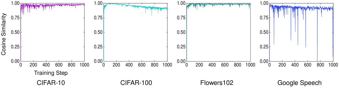
Figure 1: The cosine similarity between the latest gradient and the previous gradient. The similarities are measured for 1000 consecutive training iterations. All the curves consistently show the high similarity ($>0.8$). This observation implies that the parameter space with respect to a certain data tends not to dramatically change during training.

3.1 Key Observations on Gradient Stability

SGD-based neural network training typically goes through a large number of iterations repeatedly calculating the approximated gradients. Figure 1 shows how much the gradients are changed during training. We measure the cosine similarity between the latest gradient and the previous gradient, which are computed from the same data samples. Interestingly, the similarity remains high during the training regardless of which data and model are used. The similarity value is most likely higher than $0.85$ which indicates that the gradient is quite stable across a few consecutive iterations. In other words, the parameter space with respect to the training data does not change dramatically during the training. The similar observation has been reported in different contexts [2, 22]. This result motivates us to utilize the previous gradients for the model perturbation in SAM. Even if the previous gradient is used to perturb the model, if they are sufficiently similar to the latest one, the SAM will still be expected to improve the model’s generalization performance. We develop an asynchronous-parallel model perturbation method based on this hypothesis regarding the practical SGD dynamics.

3.2 Asynchronous-Parallel Model Perturbation with Fixed Staleness

The first step of SAM is to perturb the model through gradient ascent [8]. Once the model is perturbed, then the gradient can be computed and the model is finally updated using it. We propose to break such a data dependency between the model perturbation and the model update steps. Specifically, we asynchronously parallelize the model perturbation step such that one process calculates the gradient ascent while the other process calculates the gradient descent simultaneously. The asynchronous model perturbation can be defined as follows.

$$w_{t+1}=w_{t}-\eta\nabla L_{t}\left(w_{t}+r\frac{\nabla L_{t-\tau}(w_{t-\tau})}{\|\nabla L_{t-\tau}(w_{t-\tau})\|}\right).$$ (2)

The key difference between (2) and the original SAM is the degree of asynchrony term $\tau$ on the right-hand side. Note that, if $\tau=0$, it becomes the original SAM which can update the model only after the model is perturbed. The $\tau>0$ implies that the model is perturbed using the slightly out-of-date gradients. That is, we can update the model without waiting for the gradient ascent to be computed, which results in eliminating the extra computation time. Ideally, the training time can be the same as that of SGD that does not have a model perturbation cost.

Discussion on Gradient Staleness – While the asynchronous model perturbation (2) improves the degree of parallelism by breaking the data dependency, it may hurt the convergence properties if the gradient ascent is too inaccurate. Specifically, if $\tau$ is large, the gradient $\nabla L_{t-\tau}(w_{t-\tau})$ can be significantly different from the latest gradient $\nabla L_{t}(w_{t})$, and it results in penalizing the gradient norm less effectively. Thus, the $\tau$ should be sufficiently small to ensure the staled gradient to be similar to the latest one.

Azam et al. empirically investigated how many SGD iterations the stochastic gradients remain similar [2]. Their results show that the first-order gradients usually remain similar for roughly a decade of iterates. LookSAM proposed in [22] takes advantage of the stability of stochastic gradients such that they reuse the gradient for $k$ iterations where $k$ is a user-tunable hyper-parameter. However, the stability heavily depends on the training data as well as the learning rate, and thus cannot be simply assumed in advance. For instance, if the learning rate is large, the gradients will most likely be changed much due to the different loss landscape. Thus, it is straight-forward that the lower the degree of gradient staleness, the higher the chance of having stable gradient dynamics that is directly connected to the more effective gradient norm penalizing effect. In the following subsection, we will describe how to minimize $\tau$ without increasing the model perturbation time.

3.3 Asynchronous-Parallel Model Perturbation on Heterogeneous Systems

In modern computers, it is common to use accelerators such as GPUs to train machine learning models. Without loss of generality, we consider a system that has at least two compute resources with a different computing capability (e.g., CPU and GPU). To enable SAM algorithm to fully utilize such heterogeneous resources while maintaining the convergence properties, we propose assigning the gradient descent on the fast resource while giving the gradient ascent to the slow one. Under this general setting, the parameter update rule of SAM can be written as follows.

$$w_{t+1} =w_{t}-\eta\nabla L_{t}^{b}\left(w_{t}+r\frac{\nabla L_{t-1}^{b^{\prime}}(w_{t-1})}{\|\nabla L_{t-1}^{b^{\prime}}(w_{t-1})\|}\right),\quad b^{\prime}\leq b,$$ (3)

where $\nabla L_{t}^{b}(w_{t})$ indicates the mini-batch gradient computed from $b$ random training samples at iteration $t$ and $\nabla L_{t-1}^{b^{\prime}}(w_{t-1})$ is the mini-batch gradient computed from $b^{\prime}$ random samples at the previous iteration.

The $b^{\prime}$ directly affects how much time will be spent to compute the gradient ascent. In the original SAM, $b^{\prime}$ is assumed to be the same as $b$. We propose to adjust $b^{\prime}$ in a system-aware manner such that $b^{\prime}=(T_{f}/T_{s})\times b$. Here, $T_{s}$ is the single data gradient calculation time on the slow compute resource and $T_{f}$ is that on the fast compute resource. In this way, we can automatically find the maximum batch size $b^{\prime}$ which makes the gradient ascent time and the gradient descent time nearly the same. Such gradient ascent time can be entirely hidden behind the gradient descent time by employing a dedicated process. Note that $b^{\prime}$ will decrease as the performance difference between the two compute resources increases.

Note that $\tau$ is fixed to a constant $1$. One might think the $\tau$ could be increased instead of reducing $b^{\prime}$ to match the gradient descent time and the ascent time. Many previous works already show that they have the same complexity of the adverse impact on the convergence rate. The degree of asynchrony $\tau$ has the impact of $\mathcal{O}(\tau)$ on the convergence rate [13]. In the meantime, it has also been widely known that $\textbf{var}(\nabla L^{b})\propto b$ [10, 28]. However, reducing the batch size is more beneficial in terms of system efficiency. A smaller batch size of gradient ascent, $b^{\prime}$ reduces not only the computation time but also the memory footprint, while a greater degree of asynchrony only increases the gradient descent time that can overlap the ascent time. Therefore, we can conclude that the $\tau$ should be fixed to $1$ and the $b^{\prime}$ should be adjusted accordingly.

Algorithm 1 Asynchronous SAM with system-aware model perturbation.

1: Input: $r$: the ascent scaling factor, $T$: the number of training iterations, $b$: the gradient descent batch size, $b^{\prime}$: the gradient ascent batch size, $\eta$: the learning rate

2: for $t\in\{0,\cdots,T-1\}$ do

3:  Asynchronously compute $\nabla L^{b^{\prime}}_{t}(w_{t})$.

4:  if t $\geq$ 1 then

5:   Perturb the model: $\hat{w}_{t}=w_{t}+r\frac{\nabla L_{t-1}^{b^{\prime}}(w_{t-1})}{\|\nabla L_{t-1}^{b^{\prime}}(w_{t-1})\|}$.

6:   Compute gradient: $g_{t}=\nabla L_{t}^{b}(\hat{w}_{t})$.

7:  else

8:   Compute gradient: $g_{t}=\nabla L_{t}^{b}(w_{t})$.

9:  end if

10:  Update model: $w_{t+1}=w_{t}-\eta g_{t}$.

11: end for

12: Output: $w_{T}$

3.4 Asynchronous SAM Algorithm

We build up an asynchronous-parallel SAM by putting the aforementioned two methods together. Figure 2 shows a few schematic illustrations that support the proposed method. First, Figure 2.a shows a schematic illustration of two consecutive SAM iterations on the parameter space projected on 2-D space. The two gradient ascent steps perturb the model toward almost the same direction. This is aligned with our observation shown in Figure 1. Figure 2.b shows the schematic illustration of the proposed method. Instead of the latest gradients (red arrows), our method uses $\tau=1$ iteration-old gradients (blue arrows) for the model perturbation. Although the gradients are staled, they are still similar to the latest gradients. Thus, the model is expected to move toward a similar direction resulting in reaching the same flat minimum.

Algorithm 1 shows the proposed asynchronous SAM that corresponds to Figure 2.b. The asynchronous gradient computation at line 3 indicates the asynchronous parallel computation of the gradient for the model perturbation. Since there is no gradient for the model perturbation at the very first iteration, it runs without the perturbation. After that, the model is perturbed using $\nabla L^{b^{\prime}}_{t-1}(w_{t-1})$, the gradient computed asynchronously using 1-iteration old model parameters and $b^{\prime}$ random data samples. Note that Algorithm 1 fixes $\tau=1$. That is, the degree of staleness in the gradient ascent is minimized and it keeps the noise scale in the stochastic gradients from being too much increased when using a smaller batch size ($b^{\prime}<b$).

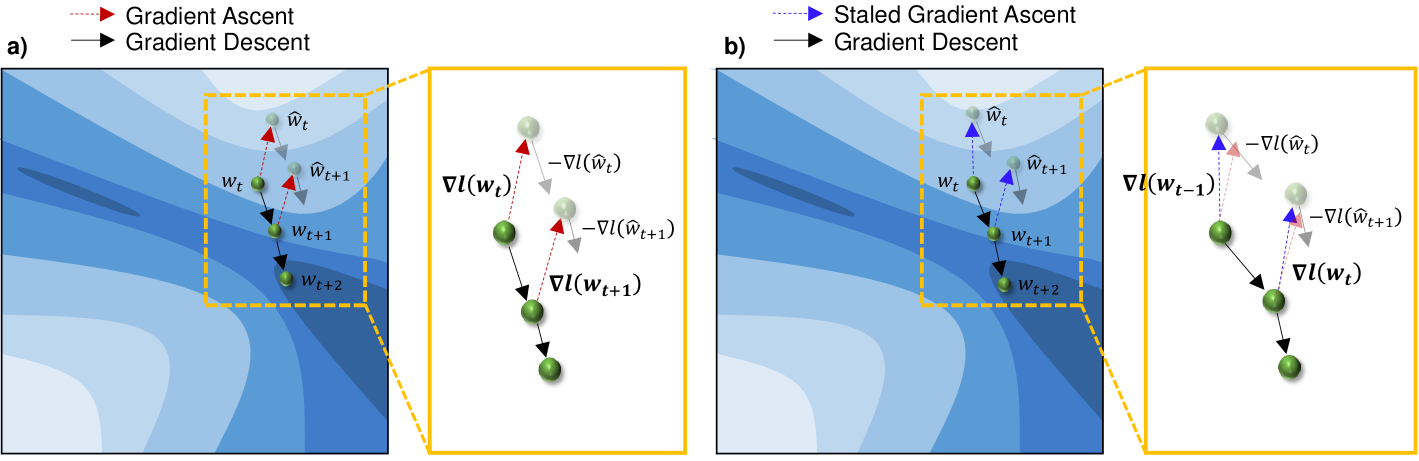
Figure 2: a: The schematic illustration of SAM. The model is updated twice using Eq. 1. The two consecutive gradients, $\nabla l(w_{t})$ and $\nabla l(w_{t+1})$ are observed to be quite similar to each other (See Fig. 1). b: The schematic illustration of the proposed asynchronous SAM. Instead of using the latest gradient for the model perturbation, the staled gradients, $\nabla l(w_{t-1})$ and $\nabla l(w_{t})$ are used to perturb $w_{t}$ and $w_{t+1}$, respectively. When $\tau$ is sufficiently small, the staled gradients are similar to the latest gradients and thus the model is expected to move toward the same minimum.

3.5 Convergence Analysis

Here we analyze the convergence behavior of the proposed asynchronous SAM with a system-aware batch size for the model perturbation. Our goal is to show that the proposed method provides a minimum performance guarantee and thus is safely applicable to real-world applications. Our analysis follows the conventional assumptions as follows.
Assumption 1. (Smoothness): There exists a constant $\beta\geq 0$ such that $\|\nabla l(u)-\nabla l(v)\|\leq\beta\|u-v\|\mathrm{,}\forall u,v\in\mathbb{R}^{d}$.
Assumption 2. (Bounded Variance): There exists a constant $\sigma\geq 0$ such that $\mathbb{E}_{\xi_{i}\in D}[\|\nabla l(w,\xi_{i})-\nabla L(w)\|^{2}]\leq\sigma^{2}$.
Assumption 3. (Bounded Norm): There exists a constant $G\geq 0$ such that $\|\nabla l(w,\xi_{i})\|^{2}\leq G^{2}\mathrm{,}\forall i\in[n]$, where $n$ is the number of total data and $\xi_{i}$ is a data sample.

Then, the convergence rate of Algorithm 1 is analyzed as follows. The proof is provided in Appendix.

Theorem 3.1.

Assume the $\beta$-smooth non-convex loss function and the bounded gradient variance and norm. Then, if $\eta\leq\frac{1}{\beta},Algorithm\ref{alg:asyncsam}satisfies:$

$$\frac{1}{T}\sum_{t=0}^{T-1}\mathbb{E}\left[\|\nabla L(w_{t})\|^{2}\right]\leq\frac{2}{T\eta}\left(L(w_{0})-\mathbb{E}\left[L(w_{T})\right]\right)+\left(\frac{2\beta^{2}r^{2}}{b^{\prime}}+\frac{4\beta^{2}r^{2}+\eta\beta}{b}\right)\sigma^{2}+4\beta^{2}r^{2}G^{2}.$$ (4)

Remark 1. Convergence guarantee: For non-convex smooth problems, Algorithm 1 guarantees a convergence regardless of which $b^{\prime}$ is used and how large $\tau$ is. When carefully choosing the learning rate $\eta$, the right-hand side can be minimized except for $\frac{2\beta^{2}r^{2}}{b^{\prime}}$, $\frac{4\beta^{2}r^{2}}{b}$, and $4\beta^{2}r^{2}G^{2}$ terms. That is, the loss will converge to a $\mathcal{O}(\beta^{2}r^{2}G^{2})$ neighborhood of the minimum. Although it does not ensure convergence to an exact minimum, this rough guarantee is acceptable and can be considered useful in real-world applications [31, 9].

Remark 2. Impact of having asynchronous gradient ascent and $b^{\prime}\leq b$: As the batch size $b^{\prime}$ decreases, the variance term on the right-hand side increases making the training loss converge more slowly. That is, if the two compute resources for the model perturbation and the model update have a significantly different capacity, the convergence rate will be more adversely affected. In addition, the right-most term on the right-hand side indicates the penalty of allowing asynchronous gradient ascent. As expected, it will converge more slowly as compared to the original SAM. However, the proposed method enables the gradient ascent time to be entirely hidden behind the gradient descent time. This trade-off between the slower convergence and the shorter end-to-end wall-clock timing will be empirically analyzed in Section 4.

4 Performance Evaluation

4.1 Experimental Settings

To evaluate the performance of our proposed asynchronous SAM, we collect and analyze the classification performance of CIFAR-10 [14] (ResNet20 [11]), CIFAR-100 (Wide-ResNet28 [30]), Oxford_Flowers102 [25] (Wide-ResNet16), Google Speech Command [29] (CNN), and Tiny-ImageNet [15] (ResNet50). We also analyze the CIFAR-100 fine-tuning performance using ImageNet-pretrained Vision Transformer (ViT) [5]. The training software is implemented using TensorFlow 2.11.0, and the experiments are conducted on several GPU machines with different CPU resources. We implement the asynchronous-parallel SAM using MPI such that two processes run in parallel, one performs the gradient ascent and the other performs the gradient descent simultaneously. The hyper-parameter settings for all individual experiments are provided in Appendix. All individual accuracy values are obtained by running at least three independent experiments.

4.2 Classification Performance

Accuracy Comparison – We first show the classification accuracy comparison in Table 4.1. We compare our method to several SOTA methods (Generalized SAM, ESAM, LookSAM, MESA, and AE-SAM) as well as the conventional SGD and the original SAM. SGD indicates mini-batch SGD with the best-tuned batch size. SAM is the vanilla SAM [8] that updates the model only using the gradients computed with the perturbed model. Generalized SAM is a variant of SAM which updates the model using both the gradient ascent and descent [33]. ESAM is a variant of SAM that takes advantage of the partial model perturbation and a biased gradient estimator [6]. LookSAM is another variant of SAM that reuses the gradient ascent [22]. MESA is a memory-efficient version of SAF(Sharpness-Aware Minimization for Free) that perturbs the model using a trajectory loss [7]. AE-SAM is also another variant of SAM that runs SGD and SAM interchangeably based on the gradient norm [12].

Overall, our proposed method achieves clearly higher accuracy than SGD. In all the benchmarks, our method’s accuracy is comparable to the generalized SAM which achieves the best validation accuracy among all the SOTA methods. A few SOTA methods achieve much lower accuracy than the original SAM (e.g., MESA in CIFAR-100 and LookSAM in Google Speech experiments) while our method consistently achieves much higher than that. These comparisons empirically prove that the proposed asynchronous-parallel model perturbation method maintains the SAM’s superior generalization performance even though the data dependency between the model perturbation and the model update is broken. It also validates that the asynchronous SAM works well not only for ResNet series with a moderate size but also for a large-scale Vision Transformer (ViT-b16).

Algorithm	CIFAR-10	CIFAR-100	Oxford Flowers102	Google Speech	CIFAR-100	Tiny-ImageNet
	(ResNet20)	(WRN-28)	(WRN-16)	(CNN)	(ViT Fine-Tuning)	(ResNet50)
SGD	$91.96\pm 0.3\%$	$79.47\pm 0.5\%$	$69.82\pm 0.2\%$	$95.96\pm 0.4\%$	$91.20\pm 0.1\%$	$61.38\pm 0.1\%$
SAM	$92.53\pm 0.4\%$	$80.13\pm 0.4\%$	$73.87\pm 0.6\%$	$97.45\pm 0.5\%$	$92.26\pm 0.1\%$	$64.68\pm 0.1\%$
Generalized SAM [33]	$92.64\pm 0.4\%$	$80.83\pm 0.5\%$	$74.77\pm 0.6\%$	$98.74\pm 0.1\%$	$92.41\pm 0.1\%$	$64.77\pm 0.3\%$
ESAM [6]	$92.59\pm 0.2\%$	$80.33\pm 0.1\%$	$74.18\pm 1.8\%$	$96.53\pm 0.2\%$	$92.08\pm 0.1\%$	$63.84\pm 0.1\%$
LookSAM [22]	$92.42\pm 0.3\%$	$80.13\pm 0.7\%$	$73.63\pm 0.5\%$	$93.94\pm 0.2\%$	$91.93\pm 0.1\%$	$61.66\pm 0.1\%$
MESA [7]	$92.22\pm 0.2\%$	$79.60\pm 0.3\%$	$74.41\pm 0.4\%$	$96.05\pm 0.4\%$	$91.35\pm 0.3\%$	-
AE-SAM [12]	$92.60\pm 0.2\%$	$80.09\pm 0.3\%$	$73.97\pm 0.7\%$	$97.38\pm 0.9\%$	$92.01\pm 0.1\%$	$63.82\pm 0.1\%$
AsyncSAM (proposed)	$92.60\pm 0.2\%$	$80.67\pm 0.5\%$	$77.70\pm 1.1\%$	$97.64\pm 1.2\%$	$91.87\pm 0.1\%$	$62.50\pm 0.1\%$

Table 4.1: The classification performance comparisons. Most of the methods outperform the baseline SGD, achieving the near accuracy to SAM. Our proposed method, AsyncSAM, shows almost the same accuracy as that of Generalized SAM which achieves the best accuracy in all the benchmarks.

One interesting result is that our method achieves significantly higher Oxford_Flowers102 accuracy than SAM. This improvement is not observed in any other benchmarks. We believe this performance gap comes from a relatively small batch size ($b=40$) and the dataset’s inherent characteristics. Finding out the specific conditions where asynchronous SAM achieves better accuracy will be crucial future work. When the model size is large, e.g., ResNet50, MESA could not successfully run on our systems due to its big memory footprint. It keeps a moving average of all the model parameters and even performs knowledge distillation using two separate models, which makes it less practical.

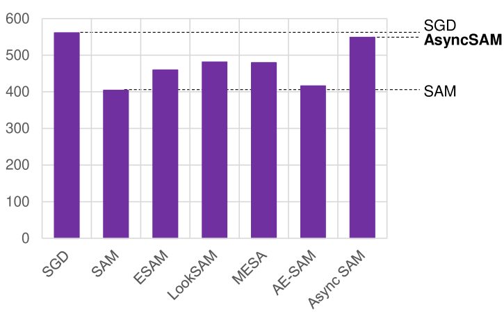
Figure 3: The CIFAR-10 training throughput Comparison (images/sec).

Throughput Comparison – Figure 3 shows the CIFAR-10 (ResNet20) training throughput comparison. The mini-batch size is set to 128 and the timing is averaged across at least 3 epochs. As expected, the original SAM shows the lowest throughput (images / sec) among all the methods. We omit Generalized SAM because it has virtually the same throughput as the original SAM (It only has one additional hyper-parameter). LookSAM, ESAM, and MESA achieve almost the same throughput that is higher than that of SAM. We clearly see that asynchronous SAM achieves remarkably higher throughput than these SOTA methods. The performance gain mostly comes from the asynchronous-parallel model perturbation method that nearly eliminates the extra computation time. Together with the model accuracy comparison shown in Table 4.1, this result verifies that asynchronous SAM maintains the model accuracy while significantly improving the system efficiency of SAM.

Time vs. Accuracy – To demonstrate the efficacy of our method, we show CIFAR-10 time-vs-accuracy curve comparison in Figure 4. Because the original SAM and the generalized SAM have exactly the same computational cost, we only show the generalized SAM which achieves higher accuracy. First, as expected, the generalized SAM takes the longest time to finish the same number of training epochs (150 in total). When using AE-SAM, SAM steps take up roughly a half of the total steps and thus it still takes much more time than SGD. It noticeably makes the training loss curve unstable, but we do not see any validation accuracy drop. We found that LookSAM significantly loses the accuracy when the gradient re-calculation interval is set to be larger than $2$. Thus, we fix it to $2$ and collected the curves. Under this setting, we see that LookSAM takes a similar amount of time as AE-SAM. Finally, our proposed asynchronous SAM takes almost the same amount of time as SGD while achieving comparable accuracy to the generalized SAM.

One interesting observation is that, while all the other variants of SAM show a slower convergence of the loss, asynchronous SAM converges even faster than SGD. We observed the same tendency across all the four benchmarks. Such an unexpected acceleration may be caused by the staleness of the gradient ascent. We consider the lack of understanding about this symptom as a limitation of this study and believe that analyzing this result and understanding the root cause will be intriguing future work.

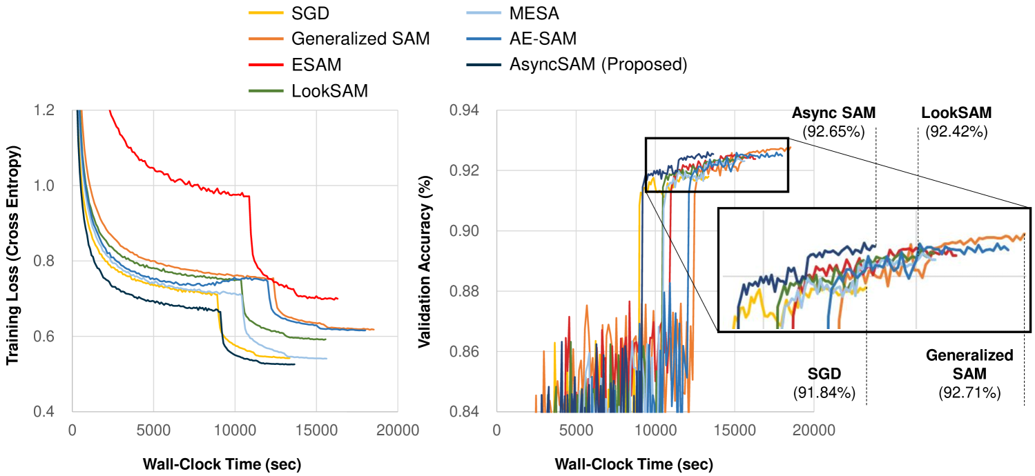
Figure 4: The CIFAR-10 learning curve comparison. Our proposed asynchronous SAM achieves nearly the same accuracy as the generalized SAM [33] while taking a similar amount of time as SGD. The generalized SAM achieves the best accuracy, however, it takes much more time than other methods. Interestingly, asynchronous SGD also achieves a training loss slightly lower than that of SGD.

Benchmark	Grad. Ascent	Grad. Descent	$\frac{b}{b^{\prime}}$	Epoch time	Valid. Accuracy
CIFAR-10	NVIDIA A6000	NVIDIA A6000	$1\times$	$91\pm 3$ sec	$92.56\pm 0.3\%$
	AMD EPYC 7452	NVIDIA A6000	$5\times$	$93\pm 3$ sec	$92.45\pm 0.4\%$
	NVIDIA RTX 4060	NVIDIA RTX 4060	$1\times$	$19\pm 1$ sec	$92.60\pm 0.6\%$
	Intel i9-13900HX	NVIDIA RTX 4060	$3\times$	$20\pm 1$ sec	$92.53\pm 0.5\%$
	Intel i7-12650H	NVIDIA RTX 4060	$4\times$	$20\pm 2$ sec	$92.47\pm 0.5\%$
Oxford_Flowers102	NVIDIA A6000	NVIDIA A6000	$1\times$	$52\pm 3$ sec	$76.49\pm 1.1\%$
	AMD EPYC 7452	NVIDIA A6000	$5\times$	$53\pm 2$ sec	$74.35\pm 0.5\%$
	NVIDIA RTX 4060	NVIDIA RTX 4060	$1\times$	$17\pm 1$ sec	$76.50\pm 0.8\%$
	Intel i9-13900HX	NVIDIA RTX 4060	$3\times$	$18\pm 1$ sec	$76.55\pm 0.3\%$
	Intel i7-12650H	NVIDIA RTX 4060	$4\times$	$18\pm 1$ sec	$74.24\pm 0.3\%$

Table 4.2: The classification performance of Asynchronous SAM on the heterogeneous system resources. The accuracy is consistently improved over SGD regardless of the system capabilities.

4.3 Performance on In-Node Heterogeneous Resources

We further support the efficacy of the proposed method by analyzing its timing and accuracy on realistic heterogeneous systems. Table 4.2 shows the average epoch time and the validation accuracy. The column $\frac{b}{b^{\prime}}$ indicates the ratio of the gradient descent batch size to the gradient ascent batch size. This value is estimated from the average iteration time in advance. First, the accuracy is consistently improved over SGD regardless of the performance gap between the in-node compute resources (See Table 4.1 for the SGD accuracy for both benchmarks). For instance, when the gradient ascent with CIFAR-10 is performed on AMD EPYC 7452, it is roughly 5 times slower than the gradient descent on NVIDIA A6000. Thus, we set $b^{\prime}=26$ while $b=128$, and asynchronous SAM still achieves $92.45\pm 0.4\%$ accuracy that is much higher than the SGD accuracy, $91.96\pm 0.3\%$. For Oxford_Flowers102, $b=40$ and $b^{\prime}$ is set to $14$ on Intel i9 and $10$ on Intel i7 depending on the performance gap. The accuracy is not dropped when $\frac{b}{b^{\prime}}\leq 3\times$, and it starts to slightly drop when the ratio goes beyond $3\times$. However, when the ratio is $5\times$, it achieves accuracy of $74.35\pm 0.5\%$ that is still significantly higher than that of SGD, $69.82\pm 0.2\%$. These results empirically prove that asynchronous SAM enables users to exploit the in-node heterogeneous system resources to improve the generalization performance.

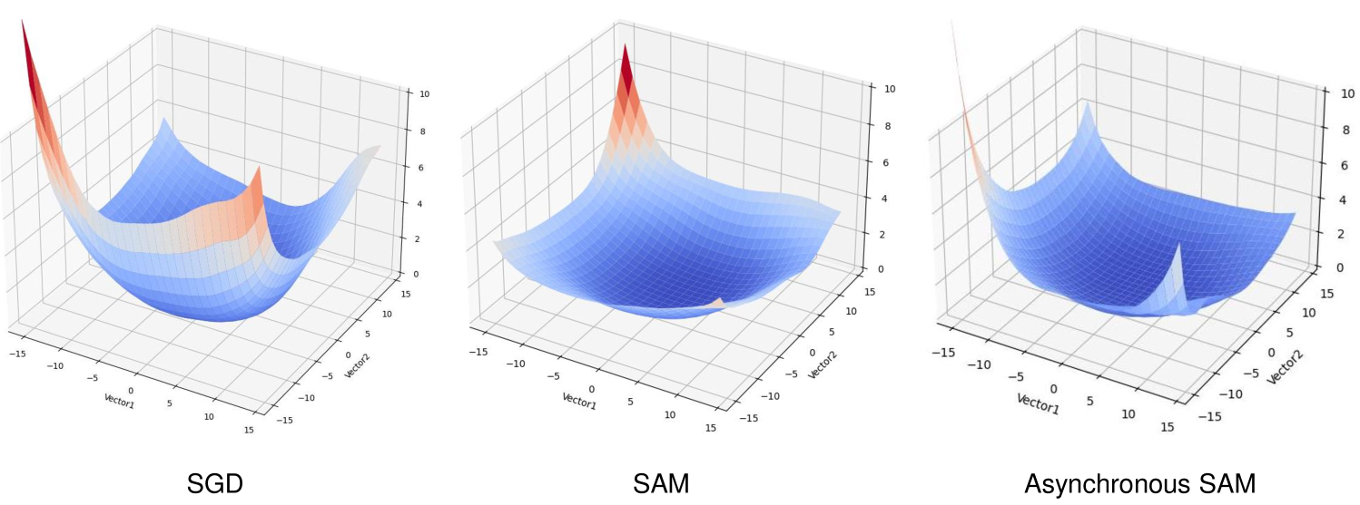
Figure 5: The CIFAR-10 loss landscape comparison. The maximum z-axis is fixed to $10$. We clearly see that asynchronous SAM leads the model to a flat region similarly to the original SAM. The flatter the loss landscape, the better the generalization performance.

4.4 Visualized Loss Landscape Comparison

We visualize the loss landscape and compare it across different SAM variants. The parameter space is visualized using the projection technique shown in [17]. We collected the loss from $30\times 30$ different points and visualized the loss landscape. To better visualize the difference, we calculated the loss directly using the logits instead of the softmax outputs. Figure 5 shows the loss landscape comparison. It is clearly shown that SAM makes the model converge to a flatter region than SGD. Likewise, asynchronous SAM shows a flatter loss landscape as compared to SGD. The corresponding validation accuracy of SGD, SAM, and asynchronous SAM are $91.83\%$, $92.61\%$, and $92.51\%$, respectively. The flatness of the loss landscape is well aligned with the achieved validation accuracy. Therefore, we can conclude that the proposed asynchronous SAM effectively leads the model to a flat region of the parameter space likely to SAM, achieving the superior generalization performance.

5 Conclusion

Our study shows that the SAM’s model perturbation time can be hidden behind the model update time by allowing a limited degree of asynchrony for the gradient ascent and carefully adjusting its batch size. Especially, it is shown that the gradient ascent computed with one-iteration-old model parameters is sufficiently accurate so that the model’s gradient norm is well penalized. This novel approach enables users to exploit heterogeneous system resources such as CPU and GPU to accelerate the neural network training with SAM. Our extensive experiments well demonstrate that the proposed method effectively reduces the training time while maintaining the superior generalization performance of SAM. In modern computers, it is common to have on CPU and multiple GPUs. Since the proposed asynchronous-parallel approach is orthogonal to the gradient recycling approach, they can be harmonized to better utilize such extremely heterogeneous system resources. Further scaling up the proposed asynchronous SAM based on the well-studied data-parallelism should be intriguing future work.

Limitations and Future Work – Our experimental results show that the asynchronous SAM loses the accuracy when the gradient ascent batch size is too small. The batch size is determined by the in-node system capacity, e.g., the performance gap between CPU and GPU. However, we verified that the accuracy drop is almost negligible when the performance gap is reasonably small. Adjusting the degree of asynchrony and the degree of stochasticity together to tackle this inaccurate gradient ascent issue will be interesting future work. In addition, our theoretical analysis is based on the bounded gradient norm assumption. We plan to improve our analysis to get rid of the strong assumption.

Appendix A Appendix

A.1 Hyper-Parameter Settings

The hyper-parameters settings used in Table 4.1 are shown in Table A.1. In addition, the optimizer-specific settings are shown in Table A.2. We believe the experiments conducted in this study can be all precisely reproduced using the above Table A.1 and A.2. If a setting is written like $x\sim y$, we choose the best one between $x$ and $y$ depending on the benchmarks.

Table A.1: The hyper-parameter settings.

Dataset	Model	Batch Size	Init. Learning Rate	Number of Epochs
CIFAR-10	ResNet20	128	0.1	150
CIFAR-100	Wide-ResNet-28	128	0.1	200
Oxford_Flowers102	Wide-ResNet-16	40	0.1	100
Google Speech	CNN	128	0.1	10
CIFAR-100	ViT-b16	40	0.01	20
Tiny-ImageNet	ResNet50	256	0.1	200

Table A.2: The optimizer-specific hyper-parameter settings.

Optimizer	Settings
SGD	momentum = $0.9$
SAM	$r=0.1$
Generalized SAM	$r=0.1$, $\alpha=0.7\sim 0.9$
ESAM	$r=0.1$, $\beta=0.6$, $\gamma=0.6\sim 1$
LookSAM	$r=0.1$, gradient ascent reuse interval = 2
MESA	$\beta=0.995$, $\lambda=0.8$, $\tau=1.5$, start epoch = 5
AE-SAM	$r=0.1$, $\lambda_{1}=-1$, $\lambda_{2}=1$, $\epsilon=0.9$
Asynchronous SAM	$r=0.05\sim 0.1$, $\tau=1$, $\frac{b}{b^{\prime}}=\{25\%,50\%,75\%,100\%\}$

A.2 Theoretical Analysis

We first present a couple of useful lemmas here. Note that our analysis borrows the proof structure used in [1].

Lemma A.1.

Given a $\beta$-smooth loss function $L(x)$, we have the following bound for any $x\in\mathbb{R}^{d}$.

$$\langle\nabla L(u)-\nabla L(v),u-v\rangle \geq-\beta\|u-v\|^{2}.$$

Proof.

Starting from the smoothness assumption,

$$\|\nabla L(u)-\nabla L(v)\|\leq\beta\|u-v\|\text{ for all }u\text{ and }v\in\mathbb{R}^{d}$$

By multiplying $\|v-u\|$ on the both side, we get

$$\|\nabla L(u)-\nabla L(v)\|\|v-u\| \leq\beta\|u-v\|\|v-u\|$$

$$\|\nabla L(u)-\nabla L(v)\|\|v-u\| \leq\beta\|u-v\|^{2}$$

$$\langle\nabla L(u)-\nabla L(v),v-u\rangle \leq\beta\|u-v\|^{2},$$ (5)

where (5) is based on Cauchy-Schwarz inequality. Then, by multiplying -1 on both sides,

$$-\langle\nabla L(u)-\nabla L(v),v-u\rangle \geq-\beta\|u-v\|^{2}$$

$$\langle\nabla L(u)-\nabla L(v),u-v\rangle \geq-\beta\|u-v\|^{2}$$

∎

Lemma A.2.

Given a $\beta$-smooth loss function $L(x)$, we have the following bound for any $r>0$ and $x\in\mathbb{R}^{d}$.

$$\langle\nabla L(w_{t}+r\nabla L(w_{t-\tau})),\nabla L(w_{t})\rangle\geq\|\nabla L(w_{t})\|^{2}-r\beta\|\nabla L(w_{t-\tau})\|^{2}$$

Proof.

$$\langle\nabla L(w_{t}+r\nabla L(w_{t-\tau})),\nabla L(w_{t})\rangle =\langle\nabla L(w_{t}+r\nabla L(w_{t-\tau}))-\nabla L(w_{t}),\nabla L(w_{t})\rangle+\|\nabla L(w_{t})\|^{2}$$

$$=\frac{1}{r}\langle\nabla L(w_{t}+r\nabla L(w_{t-\tau}))-\nabla L(w_{t}),r\nabla L(w_{t})\rangle+\|\nabla L(w_{t})\|^{2}$$

$$\geq-\frac{\beta}{r}\|r\nabla L(w_{t-\tau})\|^{2}+\|\nabla L(w_{t})\|^{2}$$ (6)

$$\geq-r\beta\|\nabla L(w_{t-\tau})\|^{2}+\|\nabla L(w_{t})\|^{2}$$

where (6) is based on Lemma A.1. ∎

Lemma A.3.

We consider the classical SAM which uses the same mini-batch when calculating the gradient ascent and the gradient descent. Then, given a $\beta$-smooth loss function $L(x)$, we have the following bound for any $r>0$, any $0\leq\kappa\leq 1$, and $x\in\mathbb{R}^{d}$.

$$\mathbb{E}\left[\langle\nabla L_{t+1}(w_{t}+r\nabla L_{t-\tau+1}(w_{t-\tau})),\nabla L(w_{t})\rangle\right]\geq\frac{1}{2}\|\nabla L(w_{t})\|^{2}-r\beta\|\nabla L(w_{t-\tau})\|^{2}-\frac{\beta^{2}r^{2}\sigma^{2}}{2b}.$$

Proof.

We first define the layer-wise gradient ascent step $\tilde{w}_{t}=w_{t}+r\nabla L(w_{t-\tau})$.

$$\mathbb{E}\left[\langle\nabla L_{t+1}(w_{t}+r\nabla L_{t-\tau+1}(w_{t-\tau})),\nabla L(w_{t})\rangle\right] =\mathbb{E}\left[\langle\nabla L(w_{t}+r\nabla L_{t-\tau+1}(w_{t-\tau})),\nabla L(w_{t})\rangle\right]$$

$$=\mathbb{E}\left[\langle\nabla L(w_{t}+r\nabla L_{t-\tau+1}(w_{t-\tau}))-\nabla L(\tilde{w}_{t})+\nabla L(\tilde{w}_{t}),\nabla L(w_{t})\rangle\right]$$

$$=\underset{E_{1}}{\underbrace{\mathbb{E}\left[\langle\nabla L(w_{t}+r\nabla L_{t-\tau+1}(w_{t-\tau}))-\nabla L(\tilde{w}_{t}),\nabla L(w_{t})\rangle\right]}}$$

$$\quad+\underset{E_{2}}{\underbrace{\mathbb{E}\left[\langle\nabla L(\tilde{w}_{t}),\nabla L(w_{t})\rangle\right]}}.$$

Then, we will bound $E_{1}$ and $E_{2}$ separately. First, $E_{1}$ is lower-bounded as follows.

$$E_{1} =\mathbb{E}\left[\langle\nabla L(w_{t}+r\nabla L_{t-\tau+1}(w_{t-\tau}))-\nabla L(\tilde{w}_{t}),\nabla L(w_{t})\rangle\right]$$

$$\geq-\frac{1}{2}\mathbb{E}\left[\|\nabla L(w_{t}+r\nabla L_{t-\tau+1}(w_{t-\tau}))-\nabla L(\tilde{w}_{t})\|^{2}\right]-\frac{1}{2}\mathbb{E}\left[\|\nabla L(w_{t})\|^{2}\right]$$

$$\geq-\frac{\beta^{2}}{2}\mathbb{E}\left[\|w_{t}+r\nabla L_{t-\tau+1}(w_{t-\tau})-\tilde{w}_{t}\|^{2}\right]-\frac{1}{2}\mathbb{E}\left[\|\nabla L(w_{t})\|^{2}\right]$$ (7)

$$=-\frac{\beta^{2}}{2}\mathbb{E}\left[\|r\nabla L_{t-\tau+1}(w_{t-\tau})-r\nabla L(w_{t-\tau})\|^{2}\right]-\frac{1}{2}\mathbb{E}\left[\|\nabla L(w_{t})\|^{2}\right]$$

$$\geq-\frac{\beta^{2}r^{2}\sigma^{2}}{2b}-\frac{1}{2}\mathbb{E}\left[\|\nabla L(w_{t})\|^{2}\right],$$ (8)

where (7) is based on the smoothness assumption. The final equality, (8), is based on the bounded variance assumption. Then, $E_{2}$ is lower-bounded directly based on Lemma A.2 as follows.

$$E_{2} =\mathbb{E}\left[\langle\nabla L(\tilde{w}_{t}),\nabla L(w_{t})\rangle\right]\geq\|\nabla L(w_{t})\|^{2}-r\beta\|\nabla L(w_{t-\tau})\|^{2}.$$

Summing up these bounds, we have

$$\mathbb{E}\left[\langle\nabla L_{t+1}(w_{t}+r\nabla L_{t-\tau+1}(w_{t-\tau})),\nabla L(w_{t})\rangle\right] =E_{1}+E_{2}$$

$$\geq\frac{1}{2}\|\nabla L(w_{t})\|^{2}-r\beta\|\nabla L(w_{t-\tau})\|^{2}-\frac{\beta^{2}r^{2}\sigma^{2}}{2b}.$$

∎

Lemma A.4.

Under the assumption of $\beta$ smoothness and the bounded variance, the SAM guarantees the following if $\eta\leq\frac{1}{\beta}$.

$$\mathbb{E}\left[L(w_{t+1})\right]\leq\mathbb{E}\left[L(w_{t})\right]-\frac{\eta}{2}\left\|\nabla L(w_{t})\right\|^{2}+\left(\frac{\eta\beta^{2}r^{2}}{b^{\prime}}+\frac{4\eta\beta^{2}r^{2}+\eta^{2}\beta}{2b}\right)\sigma^{2}+2\eta\beta^{2}r^{2}G^{2}.$$ (9)

Proof.

Let us first define the model updated with the gradient ascent as $w_{t+1/2}=w_{t}+r\nabla L_{t+1-\tau}(w_{t-\tau})$. From the smoothness assumption, we begin with the following condition.

$$L(w_{t+1})\leq L(w_{t})-\eta\langle\nabla L_{t+1}(w_{t+1/2}),\nabla L(w_{t})\rangle+\frac{\eta^{2}\beta}{2}\|\nabla L_{t+1}(w_{t+1/2})\|^{2}.$$

Taking the expectation on both sides, we have

$$\mathbb{E}\left[L(w_{t+1})\right] \leq\mathbb{E}\left[L(w_{t})\right]-\eta\mathbb{E}\left[\langle\nabla L(w_{t+1/2}),\nabla L(w_{t})\rangle\right]+\frac{\eta^{2}\beta}{2}\mathbb{E}\left[\|\nabla L_{t+1}(w_{t+1/2})\|^{2}\right]$$

$$=\mathbb{E}\left[L(w_{t})\right]-\frac{\eta}{2}\mathbb{E}\left[\left\|\nabla L(w_{t+1/2})\right\|^{2}+\left\|\nabla L(w_{t})\right\|^{2}-\underset{E_{1}}{\underbrace{\left\|\nabla L(w_{t+1/2})-\nabla L(w_{t})\right\|^{2}}}\right]$$ (10)

$$\quad+\frac{\eta^{2}\beta}{2}\underset{E_{2}}{\underbrace{\mathbb{E}\left[\|\nabla L_{t+1}(w_{t+1/2})\|^{2}\right]}}$$

Now, we focus on bounding $E_{1}$ and $E_{2}$, separately.
Bounding $E_{1}$.

$$E_{1} =\left\|\nabla L(w_{t+1/2})-\nabla L(w_{t})\right\|^{2}$$

$$\leq\beta^{2}\left\|w_{t+1/2}-w_{t}\right\|^{2}$$

$$=\beta^{2}\left\|w_{t}+r\nabla L_{t+1-\tau}(w_{t-\tau})-w_{t}\right\|^{2}$$

$$=\beta^{2}r^{2}\left\|\nabla L_{t+1-\tau}(w_{t-\tau})\right\|^{2}$$

$$=\beta^{2}r^{2}\left\|\nabla L_{t+1-\tau}(w_{t-\tau})-\nabla L(w_{t-\tau})+\nabla L(w_{t-\tau})\right\|^{2}$$

$$\leq 2\beta^{2}r^{2}\left\|\nabla L_{t+1-\tau}(w_{t-\tau})-\nabla L(w_{t-\tau})\right\|^{2}+2\beta^{2}r^{2}\left\|\nabla L(w_{t-\tau})\right\|^{2}$$

$$\leq\frac{2\beta^{2}r^{2}}{b^{\prime}}\sigma^{2}+2\beta^{2}r^{2}\left\|\nabla L(w_{t-\tau})\right\|^{2}$$

$$\leq\frac{2\beta^{2}r^{2}}{b^{\prime}}\sigma^{2}+2\beta^{2}r^{2}\left(\left\|\nabla L(w_{t-\tau})-\nabla L_{t+1}(w_{t-\tau})+\nabla L_{t+1}(w_{t-\tau})\right\|^{2}\right)$$

$$\leq\frac{2\beta^{2}r^{2}}{b^{\prime}}\sigma^{2}+4\beta^{2}r^{2}\left(\left\|\nabla L(w_{t-\tau})-\nabla L_{t+1}(w_{t-\tau})\right\|^{2}+\left\|\nabla L_{t+1}(w_{t-\tau})\right\|^{2}\right)$$

$$\leq\frac{2\beta^{2}r^{2}}{b^{\prime}}\sigma^{2}+\frac{4\beta^{2}r^{2}}{b}\sigma^{2}+4\beta^{2}r^{2}\left\|\nabla L_{t+1}(w_{t-\tau})\right\|^{2}$$

$$\leq\left(\frac{2\beta^{2}r^{2}}{b^{\prime}}+\frac{4\beta^{2}r^{2}}{b}\right)\sigma^{2}+4\beta^{2}r^{2}G^{2}$$ (11)

Bounding $E_{2}$.

$$E_{2} =\mathbb{E}\left[\|\nabla L_{t+1}(w_{t+1/2})\|^{2}\right]$$

$$=\mathbb{E}\left[\|\nabla L_{t+1}(w_{t+1/2})-\nabla L(w_{t+1/2})+\nabla L(w_{t+1/2})\|^{2}\right]$$

$$=\mathbb{E}\left[\|\nabla L_{t+1}(w_{t+1/2})-\nabla L(w_{t+1/2})\|^{2}+\|\nabla L(w_{t+1/2})\|^{2}\right]$$

$$\quad+2\left\langle\nabla L_{t+1}(w_{t+1/2})-\nabla L(w_{t+1/2}),\nabla L(w_{t+1/2})\right\rangle$$

$$=\mathbb{E}\left[\|\nabla L_{t+1}(w_{t+1/2})-\nabla L(w_{t+1/2})\|^{2}+\|\nabla L(w_{t+1/2})\|^{2}\right]$$ (12)

$$=\frac{\sigma^{2}}{b}+\mathbb{E}\left[\|\nabla L(w_{t+1/2})\|^{2}\right],$$ (13)

where (12) is based on the gradient variance assumption.

By plugging in (11) and (13) into (10), we have

$$\mathbb{E}\left[L(w_{t+1})\right] \leq\mathbb{E}\left[L(w_{t})\right]-\frac{\eta}{2}\left(\left\|\nabla L(w_{t+1/2})\right\|^{2}+\left\|\nabla L(w_{t})\right\|^{2}-\left(\frac{2\beta^{2}r^{2}}{b^{\prime}}+\frac{4\beta^{2}r^{2}}{b}\right)\sigma^{2}-4\beta^{2}r^{2}G^{2}\right)$$

$$\quad+\frac{\eta^{2}\beta}{2}\left(\frac{\sigma^{2}}{b}+\mathbb{E}\left[\|\nabla L(w_{t+1/2})\|^{2}\right]\right)$$

$$=\mathbb{E}\left[L(w_{t})\right]+\left(\frac{\eta^{2}\beta}{2}-\frac{\eta}{2}\right)\left\|\nabla L(w_{t+1/2})\right\|^{2}-\frac{\eta}{2}\left\|\nabla L(w_{t})\right\|^{2}$$

$$\quad+\left(\frac{\eta\beta^{2}r^{2}}{b^{\prime}}+\frac{2\eta\beta^{2}r^{2}}{b}+\frac{\eta^{2}\beta}{2b}\right)\sigma^{2}+2\beta^{2}r^{2}\eta G^{2}$$

$$=\mathbb{E}\left[L(w_{t})\right]-\frac{\eta}{2}\left\|\nabla L(w_{t})\right\|^{2}+\left(\frac{\eta\beta^{2}r^{2}}{b^{\prime}}+\frac{4\eta\beta^{2}r^{2}+\eta^{2}\beta}{2b}\right)\sigma^{2}+2\eta\beta^{2}r^{2}G^{2},$$ (14)

where (14) holds if $\eta\leq\frac{1}{\beta}$. ∎

Theorem A.5.

Assume the $\beta$-smooth loss function and the bounded gradient variance. Then, if $\eta\leq\frac{1}{\beta}$, mini-batch SGD satisfies:

$$\frac{1}{T}\sum_{t=0}^{T-1}\mathbb{E}\left[\|\nabla L(w_{t})\|^{2}\right]\leq\frac{2}{T\eta}\left(L(w_{0})-\mathbb{E}\left[L(w_{T})\right]\right)+\left(\frac{2\beta^{2}r^{2}}{b^{\prime}}+\frac{4\beta^{2}r^{2}+\eta\beta}{b}\right)\sigma^{2}+4\beta^{2}r^{2}G^{2}.$$ (15)

Proof.

Based on Lemma A.4, by Averaging (9) across $T$ iterates, we have

$$\frac{1}{T}\sum_{t=0}^{T-1}\mathbb{E}\left[L(w_{t+1})\right] \leq\frac{1}{T}\sum_{t=0}^{T-1}\left(\mathbb{E}\left[L(w_{t})\right]-\frac{\eta}{2}\left\|\nabla L(w_{t})\right\|^{2}+\left(\frac{\eta\beta^{2}r^{2}}{b^{\prime}}+\frac{4\eta\beta^{2}r^{2}+\eta^{2}\beta}{2b}\right)\sigma^{2}+2\eta\beta^{2}r^{2}G^{2}\right)$$

Then, we can have a telescoping sum by rearranging the terms as follows.

$$\frac{\eta}{2T}\sum_{t=0}^{T-1}\mathbb{E}\left[\|\nabla L(w_{t})\|^{2}\right] \leq\frac{1}{T}\sum_{t=0}^{T-1}\left(\mathbb{E}\left[L(w_{t})\right]-\mathbb{E}\left[L(w_{t+1})\right]\right)+\left(\frac{\eta\beta^{2}r^{2}}{b^{\prime}}+\frac{4\eta\beta^{2}r^{2}+\eta^{2}\beta}{2b}\right)\sigma^{2}+2\eta\beta^{2}r^{2}G^{2}$$

$$=\frac{1}{T}\left(L(w_{0})-\mathbb{E}\left[L(w_{T})\right]\right)+\left(\frac{\eta\beta^{2}r^{2}}{b^{\prime}}+\frac{4\eta\beta^{2}r^{2}+\eta^{2}\beta}{2b}\right)\sigma^{2}+2\eta\beta^{2}r^{2}G^{2}$$

Finally, by dividing both sides by $\frac{\eta}{2}$, we have

$$\frac{1}{T}\sum_{t=0}^{T-1}\mathbb{E}\left[\|\nabla L(w_{t})\|^{2}\right]\leq\frac{2}{T\eta}\left(L(w_{0})-\mathbb{E}\left[L(w_{T})\right]\right)+\left(\frac{2\beta^{2}r^{2}}{b^{\prime}}+\frac{4\beta^{2}r^{2}+\eta\beta}{b}\right)\sigma^{2}+4\beta^{2}r^{2}G^{2}.$$ (16)

∎

References

- Andriushchenko and Flammarion [2022] Andriushchenko, M., Flammarion, N., 2022. Towards understanding sharpness-aware minimization, in: International Conference on Machine Learning, PMLR. pp. 639–668.
- Azam et al. [2021] Azam, S.S., Hosseinalipour, S., Qiu, Q., Brinton, C., 2021. Recycling model updates in federated learning: Are gradient subspaces low-rank?, in: International Conference on Learning Representations.
- Chen et al. [2016] Chen, J., Pan, X., Monga, R., Bengio, S., Jozefowicz, R., 2016. Revisiting distributed synchronous sgd. arXiv preprint arXiv:1604.00981 .
- Cong et al. [2017] Cong, G., Bhardwaj, O., Feng, M., 2017. An efficient, distributed stochastic gradient descent algorithm for deep-learning applications, in: 2017 46th International Conference on Parallel Processing (ICPP), IEEE. pp. 11–20.
- Dosovitskiy et al. [2021] Dosovitskiy, A., Beyer, L., Kolesnikov, A., Weissenborn, D., Zhai, X., Unterthiner, T., Dehghani, M., Minderer, M., Heigold, G., Gelly, S., et al., 2021. An image is worth 16x16 words: Transformers for image recognition at scale, in: International Conference on Learning Representations.
- Du et al. [2022a] Du, J., Yan, H., Feng, J., Zhou, J.T., Zhen, L., Goh, R.S.M., Tan, V.Y., 2022a. Efficient sharpness-aware minimization for improved training of neural networks, in: International Conference on Learning Representations.
- Du et al. [2022b] Du, J., Zhou, D., Feng, J., Tan, V., Zhou, J.T., 2022b. Sharpness-aware training for free. Advances in Neural Information Processing Systems 35, 23439–23451.
- Foret et al. [2021] Foret, P., Kleiner, A., Mobahi, H., Neyshabur, B., 2021. Sharpness-aware minimization for efficiently improving generalization, in: International Conference on Learning Representations.
- Goh [2017] Goh, G., 2017. Why momentum really works. Distill 2, e6.
- Gower et al. [2019] Gower, R.M., Loizou, N., Qian, X., Sailanbayev, A., Shulgin, E., Richtárik, P., 2019. Sgd: General analysis and improved rates, in: International conference on machine learning, PMLR. pp. 5200–5209.
- He et al. [2016] He, K., Zhang, X., Ren, S., Sun, J., 2016. Deep residual learning for image recognition, in: Proceedings of the IEEE conference on computer vision and pattern recognition, pp. 770–778.
- Jiang et al. [2023] Jiang, W., Yang, H., Zhang, Y., Kwok, J., 2023. An adaptive policy to employ sharpness-aware minimization, in: International Conference on Learning Representations.
- Koloskova et al. [2022] Koloskova, A., Stich, S.U., Jaggi, M., 2022. Sharper convergence guarantees for asynchronous sgd for distributed and federated learning. Advances in Neural Information Processing Systems 35, 17202–17215.
- Krizhevsky et al. [2009] Krizhevsky, A., Hinton, G., et al., 2009. Learning multiple layers of features from tiny images. Technical Report .
- Le and Yang [2015] Le, Y., Yang, X.S., 2015. Tiny imagenet visual recognition challenge.
- Lee et al. [2024] Lee, S., Zhang, T., Prakash, S., Niu, Y., Avestimehr, S., 2024. Embracing federated learning: Enabling weak client participation via partial model training. IEEE Transactions on Mobile Computing .
- Li et al. [2018] Li, H., Xu, Z., Taylor, G., Studer, C., Goldstein, T., 2018. Visualizing the loss landscape of neural nets. Advances in neural information processing systems 31.
- Li et al. [2023] Li, Z., Cao, Q., Chen, Y., Yan, W., 2023. Cotrain: Efficient scheduling for large-model training upon gpu and cpu in parallel, in: Proceedings of the 52nd International Conference on Parallel Processing, pp. 92–101.
- Lian et al. [2015] Lian, X., Huang, Y., Li, Y., Liu, J., 2015. Asynchronous parallel stochastic gradient for nonconvex optimization. Advances in neural information processing systems 28.
- Lian et al. [2018] Lian, X., Zhang, W., Zhang, C., Liu, J., 2018. Asynchronous decentralized parallel stochastic gradient descent, in: International Conference on Machine Learning, PMLR. pp. 3043–3052.
- Liu et al. [2022a] Liu, R., Wu, F., Wu, C., Wang, Y., Lyu, L., Chen, H., Xie, X., 2022a. No one left behind: Inclusive federated learning over heterogeneous devices, in: Proceedings of the 28th ACM SIGKDD Conference on Knowledge Discovery and Data Mining, pp. 3398–3406.
- Liu et al. [2022b] Liu, Y., Mai, S., Chen, X., Hsieh, C.J., You, Y., 2022b. Towards efficient and scalable sharpness-aware minimization, in: Proceedings of the IEEE/CVF Conference on Computer Vision and Pattern Recognition, pp. 12360–12370.
- Meng et al. [2016] Meng, Q., Chen, W., Yu, J., Wang, T., Ma, Z., Liu, T.Y., 2016. Asynchronous accelerated stochastic gradient descent., in: IJCAI, pp. 1853–1859.
- Mueller et al. [2024] Mueller, M., Vlaar, T., Rolnick, D., Hein, M., 2024. Normalization layers are all that sharpness-aware minimization needs. Advances in Neural Information Processing Systems 36.
- Nilsback and Zisserman [2008] Nilsback, M.E., Zisserman, A., 2008. Automated flower classification over a large number of classes, in: Proceedings of the Indian Conference on Computer Vision, Graphics and Image Processing.
- Qu et al. [2022] Qu, Z., Li, X., Duan, R., Liu, Y., Tang, B., Lu, Z., 2022. Generalized federated learning via sharpness aware minimization, in: International Conference on Machine Learning, PMLR. pp. 18250–18280.
- Rapp et al. [2022] Rapp, M., Khalili, R., Pfeiffer, K., Henkel, J., 2022. Distreal: Distributed resource-aware learning in heterogeneous systems, in: Proceedings of the AAAI Conference on Artificial Intelligence, pp. 8062–8071.
- Smith and Le [2018] Smith, S.L., Le, Q.V., 2018. A bayesian perspective on generalization and stochastic gradient descent, in: International Conference on Learning Representations.
- Warden [2018] Warden, P., 2018. Speech commands: A dataset for limited-vocabulary speech recognition. arXiv preprint arXiv:1804.03209 .
- Zagoruyko and Komodakis [2016] Zagoruyko, S., Komodakis, N., 2016. Wide residual networks. arXiv preprint arXiv:1605.07146 .
- Zhang et al. [2021] Zhang, C., Bengio, S., Hardt, M., Recht, B., Vinyals, O., 2021. Understanding deep learning (still) requires rethinking generalization. Communications of the ACM 64, 107–115.
- Zhang et al. [2020] Zhang, X., Liu, J., Zhu, Z., 2020. Taming convergence for asynchronous stochastic gradient descent with unbounded delay in non-convex learning, in: 2020 59th IEEE Conference on Decision and Control (CDC), IEEE. pp. 3580–3585.
- Zhao et al. [2022] Zhao, Y., Zhang, H., Hu, X., 2022. Penalizing gradient norm for efficiently improving generalization in deep learning, in: International Conference on Machine Learning, PMLR. pp. 26982–26992.
- Zheng et al. [2022] Zheng, D., Song, X., Yang, C., LaSalle, D., Karypis, G., 2022. Distributed hybrid cpu and gpu training for graph neural networks on billion-scale heterogeneous graphs, in: Proceedings of the 28th ACM SIGKDD Conference on Knowledge Discovery and Data Mining, pp. 4582–4591.
- Zheng et al. [2017] Zheng, S., Meng, Q., Wang, T., Chen, W., Yu, N., Ma, Z.M., Liu, T.Y., 2017. Asynchronous stochastic gradient descent with delay compensation, in: International conference on machine learning, PMLR. pp. 4120–4129.