Refining Image Edge Detection via Linear Canonical Riesz Transforms

Abstract  Combining the linear canonical transform and the Riesz transform, we introduce the linear canonical Riesz transform (for short, LCRT), which is further proved to be a linear canonical multiplier. Using this LCRT multiplier, we conduct numerical simulations on images. Notably, the LCRT multiplier significantly reduces the complexity of the algorithm. Based on these we introduce the new concept of the sharpness $R^{\rm E}_{\rm sc}$ of the edge strength and continuity of images associated with the LCRT and, using it, we propose a new LCRT image edge detection method (for short, LCRT-IED method) and provide its mathematical foundation. Our experiments indicate that this sharpness $R^{\rm E}_{\rm sc}$ characterizes the macroscopic trend of edge variations of the image under consideration, while this new LCRT-IED method not only controls the overall edge strength and continuity of the image, but also excels in feature extraction in some local regions. These highlight the fundamental differences between the LCRT and the Riesz transform, which are precisely due to the multiparameter of the former. This new LCRT-IED method might be of significant importance for image feature extraction, image matching, and image refinement.

1 Introduction

As is well known, the Fourier transform, proposed by Joseph Fourier in 1807, was originally intended to solve the heat conduction equation. Moreover, over time, the range of applications of the Fourier transform has rapidly expanded, evolving into a key technology in scientific research and engineering. Over the course of more than two centuries, the Fourier transform has not only occupied a significant position in mathematics but has also become a cornerstone of signal processing and analysis, particularly in analyzing and processing stationary signals (see, for example, Plonka et al. [47] and Sun et al. [11, 12] for some recent applications of the Fourier transform in graph signal processing). To recall the precise definition of the Fourier transform, we denote the set of all Schwartz functions equipped with the well-known topology determined by a countable family of norms by $\mathscr{S}(\mathbb{R}^{n})$, and also by $\mathscr{S}^{\prime}(\mathbb{R}^{n})$ the set of all continuous linear functionals on $\mathscr{S}(\mathbb{R}^{n})$ equipped with the weak$-\ast$ topology.

Definition 1.1.

For any $f\in\mathscr{S}({\mathbb{R}^{n}})$, its Fourier transform $\mathscr{F}(f)$ or $\widehat{f}$ is defined by setting, for any $\boldsymbol{x}\in{\mathbb{R}^{n}}$,

$$\widehat{f}(\boldsymbol{x}):=\mathscr{F}(f)(\boldsymbol{x}):=\frac{1}{(\sqrt{2\pi})^{n}}\int_{\mathbb{R}^{n}}f(\boldsymbol{x}){e^{-i\boldsymbol{x}\cdot\boldsymbol{y}}}\,d\boldsymbol{y}$$

and its inverse Fourier transform ${f^{\vee}}$ is defined by setting, for any $\boldsymbol{x}\in{\mathbb{R}^{n}}$, $f^{\vee}(\boldsymbol{x}):=\widehat{f}(-\boldsymbol{x})$.

As the scopes and the subjects of research continue to expand, the limitations of the Fourier transform in handling non-stationary signals have become increasingly evident. These limitations manifest primarily in the following way. The Fourier transform is a global transform that provides the overall spectrum of a signal but fails to capture the local time-frequency characteristics crucial for such signals. Consequently, it cannot accurately represent the frequency behavior of signals as they evolve over time. This renders the Fourier transform inadequate for analyzing non-stationary and time-varying signals. In order to overcome these limitations, the fractional Fourier transform, the short-time Fourier transform, the Wigner distribution, and the wavelet transform were proposed. Among these, the fractional Fourier transform, as an extension of the Fourier transform, offers increased flexibility by introducing additional parameters, particularly when dealing with non-stationary signals (see, for example, [40, 56]). Notably, the research on the multidimensional fractional Fourier transform has obtained an increasing attention in recent years (see, for example, [31, 32, 33, 44, 57, 58]). To be precise, Namias [43] introduced the following multidimensional fractional Fourier transform; see also the recent monograph [56] of Zayed for a systematic study on the fractional Fourier transform.

Definition 1.2.

Let $\boldsymbol{\alpha}:=(\alpha_{1},\ldots,\alpha_{n})\in[0,2\pi)^{n}$ and $f\in\mathscr{S}(\mathbb{R}^{n})$. The fractional Fourier transform (for short, FrFT) $\mathcal{F}_{\boldsymbol{\alpha}}(f)$, with order $\boldsymbol{\alpha}$, of $f$ is defined by setting, for any $\boldsymbol{u}\in\mathbb{R}^{n}$,

$$\mathcal{F}_{\boldsymbol{\alpha}}(f)(\boldsymbol{u}):=\int_{\mathbb{R}^{n}}f(\boldsymbol{x})K_{\boldsymbol{\alpha}}(\boldsymbol{x},\boldsymbol{u})\,d\boldsymbol{x},$$

where, for any $\boldsymbol{x}:=(x_{1},\ldots,x_{n}),\boldsymbol{u}:=(u_{1},\ldots,u_{n})\in\mathbb{R}^{n}$,

$$K_{\boldsymbol{\alpha}}(\boldsymbol{x},\boldsymbol{u}):=\prod^{n}_{k=1}K_{\alpha_{k}}(x_{k},u_{k})$$

and, for any $k\in\{1,\ldots,n\}$,

$$K_{\alpha_{k}}(x_{k},u_{k}):=\left\{\begin{array}[c]{ll}\frac{c(\alpha_{k})}{\sqrt{2\pi}}e^{\pi i[a(\alpha_{k})(x_{k}^{2}+u_{k}^{2})-2b(\alpha_{k})x_{k}u_{k}]}&\quad\mathrm{if}\ \alpha_{k}\not\neq 0,\pi,\\ \delta(x_{k}-u_{k})&\quad\mathrm{if}\ \alpha_{k}=0,\\ \delta(x_{k}+u_{k})&\quad\mathrm{if}\ \alpha_{k}=\pi\end{array}\right.$$

with $a(\alpha_{k}):=\frac{\cot(\alpha_{k})}{2}$, $b(\alpha_{k}):=\csc(\alpha_{k})$, $c(\alpha_{k}):=\sqrt{1-i\cot(\alpha_{k})}$, and $\delta$ being the Dirac measure at $0$.

Observe that, when $\boldsymbol{\alpha}=(\frac{\pi}{2},\ldots,\frac{\pi}{2})$, the FrFT becomes the classical Fourier transform. The FrFT is currently employed in various fields of scientific research and engineering, including swept filters, artificial neural networks, wavelet transforms, time-frequency analysis, and complex transmission (see, for example, [10, 20, 42, 49, 52, 54]).

The linear canonical transform (for short, LCT), as an extension of the FrFT, is a more comprehensive novel mathematical transform for the analysis and the processing of non-stationary signals. The one-dimensional (for short, 1D) LCT is characterized by four parameters $\{a,b,c,d\}$, and it is also referred to as the ABCD matrix transform [5]. Additionally, the LCT is also called the generalized Fresnel transform [30], the quadratic phase system [4], and the extended FrFT [28].

In the 1D Euclidean space, the LCT features three free parameters, which enhances its flexibility compared to the FrFT. In 1961, Bargmann [2] first introduced the LCT with complex parameters. Collins [13], along with Moshinsky and Quesne [41], formally presented the LCT in the 1970s. Initially, the LCT was employed to solve differential equations and analyze optical systems. Subsequently, the relation between the LCT and existing transforms and implementation methods of the LCT in optical systems have been established (see, for example, [3, 27]). With the rapid development of the FrFT in the 1990s, the LCT gradually garnered attention in the field of signal processing. Barshan et al. [3] gave the application of the LCT in optimal filter design in 1997. Pei et al. [45] explored the discrete algorithms of the LCT, providing two types of discrete forms and applying this discrete algorithm to filter design and other areas; [46] gave the eigenvalues and the eigenfunctions of the LCT, the LCT is divided into seven cases based on different parameter assumptions, and the eigenfunctions are then applied to the self-imaging problem in optics. For more studies of LCTs, we refer to [15, 25, 26, 60].

In multidimensional signal processing, it is crucial to extend commonly used 1D signal processing tools to accommodate multidimensional signals. The multidimensional LCT is a more general form of the multidimensional Fourier transform and FrFT, and it has been widely used in various applications, including filter design, sampling, image processing, and pattern recognition (see, for example, [16, 34, 35, 48]). The multidimensional LCT was introduced in [16] as follows.

Definition 1.3.

Let $\boldsymbol{A}:=(A_{1},\ldots,A_{n})$ with the matrix $A_{k}:=\begin{bmatrix}{a_{k}}&{b_{k}}\\ {c_{k}}&{d_{k}}\end{bmatrix}\in{M_{2\times 2}}(\mathbb{R})$ ($M_{2\times 2}$ denotes the set of all $2\times 2$ real matrixes with determinant equalling 1) for any $k\in\{1,\ldots,n\}$. For any $f\in\mathscr{S}({\mathbb{R}^{n}})$, the linear canonical transform ${\mathscr{L}_{\boldsymbol{A}}}$ is defined by setting, for any $\boldsymbol{u}\in\mathbb{R}^{n}$,

$$\mathscr{L}_{\boldsymbol{A}}(f)(\boldsymbol{u}):=\int_{\mathbb{R}^{n}}f(\boldsymbol{x})K_{\boldsymbol{A}}(\boldsymbol{x},\boldsymbol{u})\,d\boldsymbol{x},$$

where, for any $\boldsymbol{x}:=(x_{1},\ldots,x_{n}),\boldsymbol{u}:=(u_{1},\ldots,u_{n})\in\mathbb{R}^{n}$,

$$K_{\boldsymbol{A}}(\boldsymbol{x},\boldsymbol{u}):=\prod^{n}_{k=1}K_{A_{k}}(x_{k},u_{k})$$

and, for any $k\in\{1,\ldots,n\}$,

$$K_{A_{k}}(x_{k},u_{k}):=\left\{\begin{array}[c]{ll}C_{A_{k}}e_{b_{k},a_{k}}({x_{k}})e_{-b_{k}}\left(x_{k},u_{k}\right)e_{b_{k},d_{k}}({u_{k}})&\quad\mathrm{if}\ b_{k}\not\neq 0,\\ \sqrt{d_{k}}e^{\frac{i}{2}\left({c_{k}}{d_{k}}u_{k}^{2}\right)}\delta(x_{k}-d_{k}u_{k})&\quad\mathrm{if}\ b_{k}=0\end{array}\right.$$

with $C_{A_{k}}:=\sqrt{\frac{1}{i2\pi b_{k}}}$, $e_{b_{k},a_{k}}({x_{k}}):=e^{i\frac{a_{k}}{2b_{k}}x_{k}^{2}}$, $e_{-b_{k}}(u_{k},x_{k}):=e^{-i{\frac{{u_{k}}{x_{k}}}{b_{k}}}}$, $e_{b_{k},d_{k}}({u_{k}}):=e^{i\frac{d_{k}}{2b_{k}}u_{k}^{2}}$, and $\delta$ as in Definition 1.2.

In Definition 1.3, when the parameter matrices $\boldsymbol{A}:=({A_{1},\ldots,A_{n}})$ take several different specific values, the LCT, as a general integral transform, reduces to several classical well-known integral transforms (see Remark 1.4). These transforms include the Fourier transform, the FrFT, the scaling operator, the chirp multiplication, and the Fresnel transform. Such transforms play a crucial role in solving problems related to electromagnetic, acoustic, and wave propagation (see, for example, [1, 6, 50]).

Remark 1.4.

Let $j\in\{1,\ldots,n\}$, $\boldsymbol{A}:=(A_{1},\ldots,A_{n})$ with $A_{j}:=\begin{bmatrix}{a_{j}}&{b_{j}}\\ {c_{j}}&{d_{j}}\end{bmatrix}\in{M_{2\times 2}}(\mathbb{R})$, and $f\in{\mathscr{S}({\mathbb{R}^{n}})}$.

1. If $A_{j}:=\begin{bmatrix}0&1\\ {-1}&0\end{bmatrix}$ for all $j$, then the LCT $\mathscr{L}_{\boldsymbol{A}}$ in this case reduces to the Fourier transform multiplied by $(\sqrt{-i})^{n}$. That is, for any $\boldsymbol{u}\in\mathbb{R}^{n}$, $\mathscr{L}_{\boldsymbol{A}}(f)(\boldsymbol{u})={(\sqrt{-i})^{n}}\mathscr{F}(f)(\boldsymbol{u})$;

2. If $A_{j}:=\begin{bmatrix}{\cos{\alpha_{j}}}\,&{\sin{\alpha_{j}}}\\ {-\sin{\alpha_{j}}}\,&{\cos{\alpha_{j}}}\end{bmatrix}$ for all $j$, then the LCT $\mathscr{L}_{\boldsymbol{A}}$ in this case reduces to the FrFT multiplied by $n$ fixed phase factors. That is, for any $\boldsymbol{u}\in\mathbb{R}^{n}$, $\mathscr{L}_{\boldsymbol{A}}(f)(\boldsymbol{u})=\prod\limits_{j=1}^{n}\sqrt{e^{-i\alpha_{j}}}\mathscr{F}_{\boldsymbol{\alpha}}(f)(\boldsymbol{u})$;

3. If $A_{j}:=\begin{bmatrix}\sigma&0\\ 0&{\frac{1}{\sigma}}\end{bmatrix}$ for all $j$, then the LCT $\mathscr{L}_{\boldsymbol{A}}$ in this case reduces to the scaling operator;

4. If $A_{j}:=\begin{bmatrix}1&\frac{z\lambda}{2\pi}\\ 0&1\end{bmatrix}$ for all $j$, then the LCT $\mathscr{L}_{\boldsymbol{A}}$ in this case reduces to the Fresenel transform, where $\lambda$ is the wave length and $z$ is the dissemination distance;

5. If $A_{j}:=\begin{bmatrix}1&0\\ {-q}&1\end{bmatrix}$ for all $j$, then the LCT $\mathscr{L}_{\boldsymbol{A}}$ in this case reduces to the chirp multiplication.

Definition 1.5.

Let $\boldsymbol{a}:=(a_{1},\ldots,a_{n}),\boldsymbol{b}:=(b_{1},\ldots,b_{n})\in\mathbb{R}^{n}$. The chirp functions $e_{\boldsymbol{a},\boldsymbol{b}}$ and $e_{\boldsymbol{a}}$ are defined, respectively, by setting, for any $\boldsymbol{x}:=(x_{1},\ldots,x_{n}),\boldsymbol{t}:=(t_{1},\ldots,t_{n})\in\mathbb{R}^{n}$,

(1.1) $${e}_{\boldsymbol{a},\boldsymbol{b}}(\boldsymbol{x}):=e^{i\sum_{j=1}^{n}\frac{b_{j}}{2a_{j}}x_{j}^{2}},$$

and

(1.2) $$e_{\boldsymbol{a}}(\boldsymbol{x},\boldsymbol{t}):=e^{i\sum_{j=1}^{n}\frac{1}{a_{j}}x_{j}t_{j}}.$$

Remark 1.6.

Let $\boldsymbol{A}:=(A_{1},\ldots,A_{n})$ with $A_{j}:=\begin{bmatrix}{{a_{j}}}&{{b_{j}}}\\ {{c_{j}}}&{{d_{j}}}\end{bmatrix}\in{M_{2\times 2}}(\mathbb{R})$ and $b_{j}\neq 0$ for any $j\in\{1,\ldots,n\}$. Define $C_{\boldsymbol{A}}:=\prod^{n}_{k=1}C_{A_{k}}$, where $C_{A_{k}}$ is the same as in Definition 1.3. Let $\boldsymbol{a}:=(a_{1},\ldots,a_{n})$, $\boldsymbol{b}:=(b_{1},\ldots,b_{n})$, $\boldsymbol{d}:=(d_{1},\ldots,d_{n})$, and $f\in{\mathscr{S}(\mathbb{R}^{n})}$. By Definitions 1.1 and 1.3, the LCT $\mathscr{L}_{\boldsymbol{A}}(f)$ of the signal $f$ is exactly the Fourier transform of the signal $g:={e}_{\boldsymbol{b},\boldsymbol{a}}f$ multiplied by the chirp functions, where ${e}_{\boldsymbol{b},\boldsymbol{a}}$ is the same as in (1.1) with exchanging the position of $\boldsymbol{a}$ and $\boldsymbol{b}$. In other words, the LCT $\mathscr{L}_{\boldsymbol{A}}(f)$ of $f$ can be decomposed into that, for any $\boldsymbol{x}\in\mathbb{R}^{n}$,

(1.3) $$\mathscr{L}_{\boldsymbol{A}}(f)(\boldsymbol{x})={\left(\sqrt{2\pi}\right)^{n}}C_{\boldsymbol{A}}{e}_{\boldsymbol{b},\boldsymbol{d}}(\boldsymbol{x})\mathscr{F}\left({e}_{\boldsymbol{b},\boldsymbol{a}}f\right)(\widetilde{\boldsymbol{x}}),$$

where ${e}_{\boldsymbol{b},\boldsymbol{d}}$ is the same as in (1.1) with $\boldsymbol{a}$ and $\boldsymbol{b}$ replaced, respectively, by $\boldsymbol{b}$ and $\boldsymbol{d}$ and where $\boldsymbol{\widetilde{x}}:=\frac{\boldsymbol{x}}{\boldsymbol{b}}:=(\frac{x_{1}}{b_{1}},\ldots,\frac{x_{n}}{b_{n}})$. Based on (1.3), we observe that the LCT $\mathscr{L}_{\boldsymbol{A}}(f)$ of a function $f\in{\mathscr{S}(\mathbb{R}^{n})}$ consists of the following four simpler operators (as illustrated in Figure 1):

1. The multiplication by a chirp function, that is, for any $\boldsymbol{t}\in\mathbb{R}^{n}$, $g(\boldsymbol{t}):={e}_{\boldsymbol{b},\boldsymbol{a}}f(\boldsymbol{t})$;

2. The Fourier transform, that is, for any $\boldsymbol{x}\in\mathbb{R}^{n}$, $\widehat{g}(\boldsymbol{x}):=(\mathscr{F}g)(\boldsymbol{x})$;

3. The scaling operator, that is, for any $\boldsymbol{x}\in\mathbb{R}^{n}$, $\widetilde{g}(\boldsymbol{x}):=g(\frac{\boldsymbol{x}}{\boldsymbol{b}})$;

4. The multiplication by a chirp function again, that is, for any $\boldsymbol{x}\in\mathbb{R}^{n}$,

   $$\mathscr{L}_{A}(f)(\boldsymbol{x}):=\left(\sqrt{2\pi}\right)^{n}{C_{A}}{{e}_{\boldsymbol{b},\boldsymbol{d}}}\widetilde{g}(\boldsymbol{x}).$$

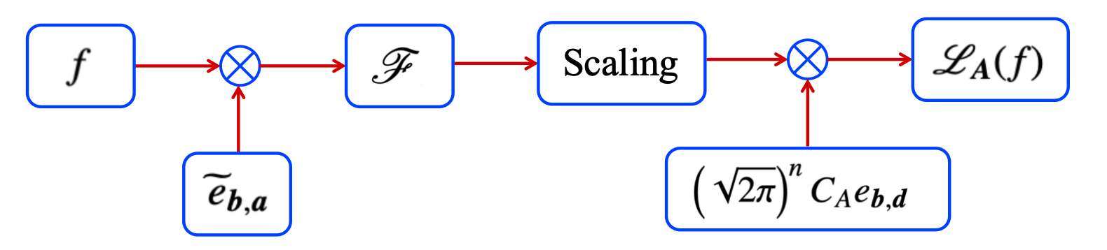
Figure 1: The decomposition of the LCT $\mathscr{L}_{\boldsymbol{A}}$.

The definition of the multidimensional inverse LCT in [39] is as follows.

Definition 1.7.

Let $\boldsymbol{A}:=(A_{1},\ldots,A_{n})$ and $\boldsymbol{A}^{-1}:=(A_{1}^{-1},\ldots,A_{n}^{-1})$, respectively, with the matrices $A_{k}:=\begin{bmatrix}{a_{k}}&{b_{k}}\\ {c_{k}}&{d_{k}}\end{bmatrix},A_{k}^{-1}:=\begin{bmatrix}{d_{k}}&{-b_{k}}\\ {-c_{k}}&{\ a_{k}}\end{bmatrix}\in{M_{2\times 2}}(\mathbb{R})$ for any $k\in\{1,\ldots,n\}$. For any $f\in\mathscr{S}(\mathbb{R}^{n})$, its multidimensional inverse LCT $({\mathscr{L}_{\boldsymbol{A}}})^{-1}(f)$ is defined by setting, for any $\boldsymbol{x}\in\mathbb{R}^{n}$, $\left({\mathscr{L}_{\boldsymbol{A}}}\right)^{-1}(f)(\boldsymbol{x}):={\mathscr{L}_{\boldsymbol{A}^{-1}}}(f)(\boldsymbol{x}).$

The Hilbert transform occupies a significant position in Fourier analysis and plays a crucial role in signal processing. It has been extensively applied to modulation theory, edge detection, and filter design (see, for example, [7, 8, 21, 47]). In recent years, the FrFT and the LCT are respectively combined with the Hilbert transform to lead to the fractional Hilbert transform and the linear canonical Hilbert transform (for short, LCHT), which yield significant results (see, for example, [10, 55]). The Riesz transform serves as a natural extension of the Hilbert transform in the $n$-dimensional Euclidean space. In 2023, Fu et al. [19] combined the FrFT with the Riesz transform, introducing the fractional Riesz transform and applying it to edge detection. Compared to the classical Riesz transform, the fractional Riesz transform is capable of detecting not only global information in images but also local information in arbitrary directions.

In this article, combining the linear canonical transform and the Riesz transform, we introduce the linear canonical Riesz transform (for short, LCRT), which is further proved to be a linear canonical multiplier. Using this LCRT multiplier, we conduct numerical simulations on images. Notably, the LCRT multiplier significantly reduces the complexity of the algorithm. Based on these we introduce the new concept of the sharpness $R^{\rm E}_{\rm sc}$ of the edge strength and continuity of images associated with the LCRT and, using it, we propose a new LCRT image edge detection method (for short, LCRT-IED method) and provide its mathematical foundation. Our experiments indicate that this sharpness $R^{\rm E}_{\rm sc}$ characterizes the macroscopic trend of edge variations of the image under consideration, while this new LCRT-IED method not only controls the overall edge strength and continuity of the image, but also excels in feature extraction in some local regions. These highlight the fundamental differences between the LCRT and the Riesz transform, which are precisely due to the multiparameter of the former. This new LCRT-IED method might be of significant importance for image feature extraction, image matching, and image refinement.

The remainder of this article is organized as follows.

In Section 2, we introduce the LCRT and prove that the LCRT is the linear canonical multiplier (Theorem 2.7). Additionally, we obtain the boundedness of the LCRT on Lebesgue spaces (Theorem 2.10).

In Section 3, we conduct numerical simulations of images using the LCRT, demonstrating the image of the original test image (Gaussian function) after the LCRT (Figure 4) and, in the LCT domain, the amplitude, the real part, and the imaginary part of both the original test image and the image after the LCRT (Figures 5 and 6). The obtained results demonstrate that the LCRT exhibits both the amplitude attenuate and the shifting effect in the LCT domain. Additionally, we conduct image numerical simulations of the LCHT to compare the differences between the multiplier of the LCHT and the LCRT (Figure 7).

In Section 4, we first introduce the new concept of the sharpness $R^{\rm E}_{\rm sc}$ of the edge strength and continuity of images associated with the LCRT in Definition 4.1. Based on this we then propose the new LCRT-IED method and provide its mathematical foundation (Theorem 4.2). This sharpness $R^{\rm E}_{\rm sc}$ is used to characterize the macroscopic trend of edge changes in the image under consideration. Our experimental results (Figures 8, 9, 10, 11, 12, and 13 and Tables 1, 2, and 3) demonstrate that the LCRT-IED method can gradually control of the edge strength and continuity by subtly adjusting the parameter matrices of the LCRT. Additionally, this new LCRT-IED method also demonstrates its capabilities in feature extraction within some local regions, enabling better preservation of image details. Also, in this section, we further summarize the advantages and features of this new LCRT-IED method in image processing.

A conclusion is given in Section 5.

It is worth mentioning that the experimental results presented in this article do not require the final binarization like the fractional Riesz transform edge detection method in [19] and, moreover, the results are equally striking. This can be attributed to the fact that the LCT is able to perform not only rotations but also scaling operations in the time-frequency plane. Furthermore, this new LCRT-IED method also performs exceptionally well when processing RGB images.

Finally, we make some conventions on notation. Let $\mathbb{N}:=\{1,2,\ldots\}$, ${C}^{\infty}({\mathbb{R}^{n}})$ denote the set of all infinitely differentiable functions on $\mathbb{R}^{n}$. We use $C$ to denote a positive constant, which is independent of the main parameters involved, whose value may vary from line to line. The symbol $g\lesssim h$ means $g\leq Ch$. If $g\lesssim h$ and $h\lesssim g$, we then write $g\sim h$. Let $p\in(0,\infty]$. The Lebesgue space $L^{p}(\mathbb{R}^{n})$ is defined to be the set of all measurable functions $f$ on $\mathbb{R}^{n}$ such that, when $p\in(0,\infty)$, $\|f\|_{L^{p}(\mathbb{R}^{n})}:=\left[\int_{\mathbb{R}^{n}}|f(x)|^{p}\,dx\right]^{\frac{1}{p}}<\infty$ and

$$\|f\|_{L^{\infty}(\mathbb{R}^{n})}:=\mathop{\mathrm{\,ess\,sup\,}}_{x\in\mathbb{R}^{n}}|f(x)|<\infty.$$

Moreover, when we prove a theorem (and the like), in its proof we always use the same symbols as those used in the statement itself of that theorem (and the like).

2 Linear Canonical Riesz Transforms

The Riesz transform, as a natural extension of the Hilbert transform in the $n$-dimensional Euclidean space, is the archetype of Calderón–Zygmund operators, which is not only an important class of convolution operators but also a special class of Fourier multipliers. The fractional Hilbert transform and the LCHT have been extensively studied and widely applied in signal processing (see, for example, [18, 28, 53, 59]). The LCHT was introduced by Li et al. in [38] as follows.

Definition 2.1.

Let $A:=\begin{bmatrix}a&b\\ c&d\end{bmatrix}\in{M_{2\times 2}}(\mathbb{R})$ and $b\neq 0$. The linear canonical Hilbert transform (for short, LCHT) ${H_{A}}$ is defined by setting, for any $f\in\mathscr{S}({\mathbb{R}})$ and $t\in{\mathbb{R}}$,

$${H_{A}}(f)(t):=\frac{1}{\pi}e^{-i\frac{d}{2b}{t^{2}}}{\rm p}.{\rm v}.\int_{\mathbb{R}}{\frac{f(x)e^{i\frac{a}{2b}{x^{2}}}}{t-x}\,dx}.$$

Remark 2.2.

If $A:=\begin{bmatrix}{\cos{\alpha}\,}&{\sin{\alpha}}\\ {-\sin{\alpha}\,}&{\cos{\alpha}}\end{bmatrix}$ with $\alpha\in(0,2\pi)$ and $\alpha\neq\pi$, then the LCHT reduces to the fractional Hilbert transform in [55, Definition 1].

The two-dimensional (for short, 2D) half-planed Hilbert transform was introduced by Xu et al. in [53] as follows.

Definition 2.3.

Let $A_{j}:=\begin{bmatrix}{a_{j}}&{b_{j}}\\ {c_{j}}&{d_{j}}\end{bmatrix}\in{M_{2\times 2}}(\mathbb{R})$ and $b_{j}\neq 0$ for any $j\in\{1,2\}$. The half-planed Hilbert transforms related to the LCT (for short, HLCHT) $H_{x}^{A_{1}}$ and $H_{y}^{A_{2}}$ are defined by setting, for any $f\in\mathscr{S}({\mathbb{R}^{2}})$ and $x,y\in\mathbb{R}$,

$$H_{x}^{A_{1}}\left(f\right)\left({x,y}\right):=\frac{e^{\frac{-id_{1}x^{2}}{2b_{1}}}}{\pi}{\rm p}.{\rm v}.\int_{\mathbb{R}}\frac{f(\xi,y)e^{\frac{-ia_{1}\xi^{2}}{2b_{1}}}}{x-\xi}\,d\xi$$

and

$$H_{y}^{A_{2}}\left(f\right)\left({x,y}\right):=\frac{e^{\frac{-id_{2}y^{2}}{2b_{2}}}}{\pi}{\rm p}.{\rm v}.\int_{\mathbb{R}}\frac{f(x,\eta)e^{\frac{-ia_{2}\eta^{2}}{2b_{2}}}}{y-\eta}\,d\eta,$$

where $H_{x}^{A_{1}}$ is the HLCHT along $X$ axis and $H_{y}^{A_{2}}$ is the HLCHT along $Y$ axis.

Fu et al. [19] further extended the concept of fractional Hilbert transforms to higher dimensions, referred to as the fractional Riesz transforms, and successfully applied this extension to image edge detection. Compared with the classical Riesz transform used in edge detection, the fractional Riesz transform not only extracts global edge information from images but also flexibly captures local edge information in any directions by adjusting the fractional parameters.

Definition 2.4.

(see [19]) For any $j\in\{1,\ldots,n\}$ and $\boldsymbol{\alpha}:=(\alpha_{1},\ldots,\alpha_{n})\in[0,2\pi)^{n}$ with $\alpha_{k}\notin\{0,\pi\}$ for any $k\in\{1,\ldots,n\}$, the $j$th fractional Riesz transform $R_{j}^{\boldsymbol{\alpha}}(f)$ of $f\in\mathscr{S}(\mathbb{R}^{n})$ is defined by setting, for any $\boldsymbol{x}\in\mathbb{R}^{n}$,

$$R_{j}^{\boldsymbol{\alpha}}(f)(\boldsymbol{x}):=\widetilde{c}_{n}\ {\rm p}.{\rm v}.\ e_{-\boldsymbol{\alpha}}(\boldsymbol{x})\int_{\mathbb{R}^{n}}\frac{x_{j}-y_{j}}{|\boldsymbol{x}-\boldsymbol{y}|^{n+1}}f(\boldsymbol{y})e_{\boldsymbol{\alpha}}(\boldsymbol{y})\,d\boldsymbol{y},$$

where $\widetilde{c}_{n}:=\Gamma(\frac{n+1}{2})/\pi^{\frac{n+1}{2}}$, $e_{\boldsymbol{\alpha}}(\boldsymbol{x}):=e^{i\sum\nolimits_{k=1}^{n}\frac{\cot({\alpha_{k}})}{2}{x_{k}^{2}}}$, and $e_{-\boldsymbol{\alpha}}(\boldsymbol{x}):=e^{-i\sum\nolimits_{k=1}^{n}\frac{\cot({\alpha_{k}})}{2}{x_{k}^{2}}}$.

In other words, the fractional Riesz transform can also be viewed as a fractional convolution operator. Fu et al. [19] proved that the fractional Riesz transform is a fractional multiplier, demonstrating that the fractional Riesz transform is entirely equivalent to the composition of the FrFT, the fractional multiplier, and the inverse FrFT.

Based on the LCHT and the fractional Riesz transform, we introduce the $j$th linear canonical Riesz transform as follows.

Definition 2.5.

Let $\boldsymbol{A}:=(A_{1},\ldots,A_{n})$ with $A_{k}:=\begin{bmatrix}{a_{k}}&{b_{k}}\\ {c_{k}}&{d_{k}}\end{bmatrix}\in{M_{2\times 2}}(\mathbb{R})$ and $b_{k}\neq 0$ for any $k\in\{1,\ldots,n\}$, and let $\boldsymbol{a}:=(a_{1},\ldots,a_{n})$, $\boldsymbol{b}:=(b_{1},\ldots,b_{n})$, and $\boldsymbol{d}:=(d_{1},\ldots,d_{n})$. For any given $j\in\{1,\ldots,n\}$, the $j$th linear canonical Riesz transform (for short, LCRT) $R_{j}^{\boldsymbol{A}}(f)$ of $f\in\mathscr{S}(\mathbb{R}^{n})$ is defined by setting, for any $\boldsymbol{x}\in\mathbb{R}^{n}$,

(2.1) $$R_{j}^{\boldsymbol{A}}(f)(\boldsymbol{x}):={\widetilde{c}_{n}}{e}_{\boldsymbol{b},-\boldsymbol{d}}(\boldsymbol{x})\,{\rm p}.{\rm v}.\int_{\mathbb{R}^{n}}\frac{({x_{j}}-{y_{j}})f(\boldsymbol{y}){e}_{\boldsymbol{b},\boldsymbol{a}}(\boldsymbol{y})}{|\boldsymbol{x}-\boldsymbol{y}|^{n+1}}\,d\boldsymbol{y},$$

where $\widetilde{c}_{n}:=\frac{\Gamma(\frac{n+1}{2})}{\pi^{\frac{n+1}{2}}}$, ${e}_{\boldsymbol{b},-\boldsymbol{d}}$ is the same as in (1.1) with $\boldsymbol{a}$ and $\boldsymbol{b}$ replaced, respectively, by $\boldsymbol{b}$ and $-\boldsymbol{d}$ and ${e}_{\boldsymbol{b},\boldsymbol{a}}$ is the same as in (1.1) with exchanging the position of $\boldsymbol{a}$ and $\boldsymbol{b}$.

Remark 2.6.

1. Let $k,j\in\{1,\ldots,n\}$. If $\boldsymbol{A}:=({{A_{1}},\ldots,{A_{n}}})$ with $A_{k}:=\begin{bmatrix}\cos{\alpha_{k}}&\sin{\alpha_{k}}\\ -\sin{\alpha_{k}}&\cos{\alpha_{k}}\end{bmatrix}$ and both $\alpha_{k}\in(0,2\pi)$ and $\alpha_{k}\neq\pi$, then the LCRT $R_{j}^{\boldsymbol{A}}$ in this case becomes the fractional Riesz transform $R_{j}^{\boldsymbol{\alpha}}$ in [19, Definition 1.3]. If $\boldsymbol{A}:=({{A_{1}},\ldots,{A_{n}}})$ with $A_{k}:=\begin{bmatrix}0&1\\ {-1}&0\end{bmatrix}$ for all $k$, then the LCRT $R_{j}^{\boldsymbol{A}}$ in this case becomes the classical Riesz transform $R_{j}$ in [24, Definition 4.1.13].

2. If $n=1$, then the LCRT becomes the LCHT in this case in [38, (7), Section 2].

Now, we prove that the LCRT is a linear canonical multiplier, which demonstrates that the LCRT is equivalent to the composition of the LCT and a multiplier.

Theorem 2.7.

Let $k,j\in\{1,\ldots,n\}$ and $\boldsymbol{A}:=(A_{1},\ldots,A_{n})$ with $A_{k}:=\begin{bmatrix}{a_{k}}&{b_{k}}\\ {c_{k}}&{d_{k}}\end{bmatrix}\in{M_{2\times 2}}(\mathbb{R})$ and both $b_{k}\neq 0$ and $a_{k}=d_{k}$ for all $k$, and let $\boldsymbol{a}:=(a_{1},\ldots,a_{n})$, $\boldsymbol{b}:=(b_{1},\ldots,b_{n})$, and $\boldsymbol{d}:=(d_{1},\ldots,d_{n})$. From the perspective of the LCT, the $j$th LCRT $R_{j}^{\boldsymbol{A}}$ is given by the multiplication by the function $\frac{-i\omega_{j}}{b_{j}}/{|\frac{\boldsymbol{\omega}}{\boldsymbol{b}}|}$. That is, for any $f\in\mathscr{S}(\mathbb{R}^{n})$ and $\boldsymbol{\omega}\in\mathbb{R}^{n}$, one has

(2.2) $$\mathscr{L}_{\boldsymbol{A}}\left[R_{j}^{\boldsymbol{A}}(f)\right](\boldsymbol{\omega})=-i\frac{\frac{\omega_{j}}{b_{j}}}{|\frac{\boldsymbol{\omega}}{\boldsymbol{b}}|}\mathscr{L}_{\boldsymbol{A}}(f)(\boldsymbol{\omega}),$$

where $\frac{\boldsymbol{\omega}}{\boldsymbol{b}}:=(\frac{\omega_{1}}{b_{1}},\ldots,\frac{\omega_{n}}{b_{n}})$.

Proof.

From the definitions of LCTs and LCRTs, it follows that, for any $f\in\mathscr{S}(\mathbb{R}^{n})$ and $\boldsymbol{\omega}\in\mathbb{R}^{n}$,

(2.3) $$\mathscr{L}_{\boldsymbol{A}}\left[R_{j}^{\boldsymbol{A}}\left(f\right)\right](\boldsymbol{\omega})$$

$$\quad={\widetilde{c}_{n}}\int_{\mathbb{R}^{n}}{e}_{-\boldsymbol{b},\boldsymbol{d}}\left(\boldsymbol{t}\right)\lim_{\varepsilon\rightarrow 0}\int_{|\boldsymbol{t}-\boldsymbol{x}|\geq\varepsilon}{\frac{({t_{j}}-{x_{j}})f(\boldsymbol{x}){e}_{\boldsymbol{b},\boldsymbol{a}}\left(\boldsymbol{x}\right)}{{|{\boldsymbol{t}-\boldsymbol{x}}|}^{n+1}}\,d\boldsymbol{x}}K_{\boldsymbol{A}}(\boldsymbol{t},\boldsymbol{\omega})\,d\boldsymbol{t}$$

$$\quad=C_{\boldsymbol{A}}\int_{\mathbb{R}^{n}}{f\left(\boldsymbol{x}\right)}{e}_{\boldsymbol{b},\boldsymbol{a}}\left(\boldsymbol{\omega}\right){e}_{\boldsymbol{b},\boldsymbol{a}}\left(\boldsymbol{x}\right)\left[\frac{\Gamma\left(\frac{n+1}{2}\right)}{\pi^{\frac{n+1}{2}}}\lim_{\varepsilon\rightarrow 0}\int_{|\boldsymbol{t}-\boldsymbol{x}|\geq\varepsilon}{\frac{(t_{j}-x_{j}){e_{-\boldsymbol{b}}}\left(\boldsymbol{t},\boldsymbol{\omega}\right)}{{|\boldsymbol{t}-\boldsymbol{x}|}^{n+1}}\,d\boldsymbol{t}}\right]\,d\boldsymbol{x},$$

where ${e}_{\boldsymbol{b},\boldsymbol{a}}$ is the same as in (1.1) with exchanging the position of $\boldsymbol{a}$ and $\boldsymbol{b}$ and $e_{-\boldsymbol{b}}$ is the same as in (1.2) with $\boldsymbol{a}$ replaced by $-\boldsymbol{b}$. Let

$$I:=\frac{\Gamma\left(\frac{n+1}{2}\right)}{\pi^{\frac{n+1}{2}}}\lim_{\varepsilon\rightarrow 0^{+}}\int_{|\boldsymbol{t}-\boldsymbol{x}|\geq\varepsilon}\frac{(t_{j}-x_{j})e_{-\boldsymbol{b}}({\boldsymbol{t},\boldsymbol{\omega}})}{{|\boldsymbol{t}-\boldsymbol{x}|}^{n+1}}d\boldsymbol{t},$$

here and thereafter, $\varepsilon\rightarrow 0^{+}$ means $\varepsilon\in(0,c_{0})$, with $c_{0}$ being some positive constant, and $\varepsilon\rightarrow 0$. By a change of variables and the spherical coordinate transformation, we conclude that

$$I =-\frac{\Gamma(\frac{n+1}{2})}{\pi^{\frac{n+1}{2}}}\lim_{\varepsilon\rightarrow 0^{+}}\int_{|\boldsymbol{t}-\boldsymbol{x}|\geq\varepsilon}\frac{(x_{j}-t_{j})e_{-\boldsymbol{b}}(\boldsymbol{t},\boldsymbol{\omega})}{|\boldsymbol{x}-\boldsymbol{t}|^{n+1}}\,d\boldsymbol{t}$$

$$=-\frac{\Gamma(\frac{n+1}{2})}{\pi^{\frac{n+1}{2}}}\lim_{\varepsilon\rightarrow 0^{+}}\int_{|\boldsymbol{y}|\geq\varepsilon}\frac{y_{j}e^{-i\sum\limits_{j=1}^{n}\frac{(x_{j}-y_{j})\omega_{j}}{b_{j}}}}{{|\boldsymbol{y}|}^{n+1}}\,d\boldsymbol{y}$$

$$=-\frac{\Gamma(\frac{n+1}{2})}{\pi^{\frac{n+1}{2}}}e^{-i\sum\limits_{j=1}^{n}{\frac{{x_{j}}{\omega_{j}}}{b_{j}}}}\lim_{\varepsilon\rightarrow 0}\int_{s^{n-1}}\int_{\varepsilon\leq r\leq\frac{1}{\varepsilon}}{e^{i\sum\limits_{j=1}^{n}{\frac{{r{\theta_{j}}{\omega_{j}}}}{b_{j}}}}\frac{1}{r}}{\theta_{j}}\,dr\,d\boldsymbol{\theta}$$

$$=-\frac{\Gamma({\frac{n+1}{2}})}{\pi^{\frac{n+1}{2}}}e^{-i\sum\limits_{j=1}^{n}{\frac{x_{j}{\omega_{j}}}{b_{j}}}}\int_{S^{n-1}}{\int_{0}^{\infty}i\frac{\sin(\sum\limits_{j=1}^{n}{\frac{r{\theta_{j}}{\omega_{j}}}{b_{j}}})}{r}}{\theta_{j}}\,dr\,d\boldsymbol{\theta}$$

$$=-\frac{\Gamma(\frac{n+1}{2})}{\pi^{\frac{n+1}{2}}}e^{-i\sum\limits_{j=1}^{n}{\frac{x_{j}{\omega_{j}}}{b_{j}}}}\int_{S^{n-1}}{\int_{0}^{\infty}i\frac{{}^{\sin(r\sum\limits_{j=1}^{n}{\frac{\theta_{j}\omega_{j}}{b_{j}}})}}{r\sum\limits_{j=1}^{n}\frac{\theta_{j}\omega_{j}}{b_{j}}}}{\theta_{j}}d\left(\sum\limits_{j=1}^{n}{\frac{\theta_{j}\omega_{j}}{b_{j}}}r\right)\,d\boldsymbol{\theta}$$

$$=-i\frac{\Gamma({\frac{n+1}{2}})}{\pi^{\frac{n+1}{2}}}e^{-i\sum\limits_{j=1}^{n}\frac{x_{j}{\omega_{j}}}{b_{j}}}\frac{1}{2}\pi\frac{2\pi^{\frac{n-1}{2}}}{\Gamma\left(\frac{n+1}{2}\right)}\frac{\frac{\omega_{j}}{b_{j}}}{\left|{\frac{\boldsymbol{\omega}}{\boldsymbol{b}}}\right|}=-ie^{-i\sum\limits_{j=1}^{n}\frac{x_{j}{\omega_{j}}}{b_{j}}}\frac{\frac{\omega_{j}}{b_{j}}}{|{\frac{\boldsymbol{\omega}}{\boldsymbol{b}}}|}.$$

Substituting the above formula into (2.3), we then obtain

$$\mathscr{L}_{\boldsymbol{A}}\left[R_{j}^{\boldsymbol{A}}\left(f\right)\right](\boldsymbol{\omega}) =-iC_{\boldsymbol{A}}\int_{\mathbb{R}^{n}}f(\boldsymbol{x})e^{i\sum\limits_{j=1}^{n}({\frac{a_{j}}{2b_{j}}\omega_{j}^{2}-\frac{x_{j}{\omega_{j}}}{b_{j}}+\frac{a_{j}}{{2b_{j}}}x_{j}^{2}})}\frac{\frac{\omega_{j}}{b_{j}}}{\left|{\boldsymbol{\frac{\omega}{b}}}\right|}\,d\boldsymbol{x}=-i\frac{{\frac{\omega_{j}}{b_{j}}}}{|{\frac{\boldsymbol{\omega}}{\boldsymbol{b}}}|}{\mathscr{L}_{\boldsymbol{A}}}(f)(\boldsymbol{\omega}).$$

This finishes the proof of Theorem 2.7. ∎

Remark 2.8.

1. When $n=1$, Theorem 2.7 in this case coincides with [38, Theorem 2] which is on the LCHT.

2. Let $j\in\{1,\ldots,n\}$. When $A_{j}:=\begin{bmatrix}{\cos{\alpha_{j}}}&{\sin{\alpha_{j}}}\\ {-\sin{\alpha_{j}}}&{\cos{\alpha_{j}}}\end{bmatrix}$ with $\alpha_{j}\in(0,2\pi)$ and $\alpha_{j}\neq\pi$, Theorem 2.7 in this case reduces to [19, Theorem 2.1] which is on the fractional Riesz transform.

The following lemma gives the inverse LCT theorem, which is precisely [16, Reversible property (13)].

Lemma 2.9.

Let $\boldsymbol{A}:=(A_{1},\ldots,A_{n})$ with $A_{k}:=\begin{bmatrix}{a_{k}}&{b_{k}}\\ {c_{k}}&{d_{k}}\end{bmatrix}\in{M_{2\times 2}}(\mathbb{R})$ for any $k\in\{1,\ldots,n\}$. For any $f\in\mathscr{S}(\mathbb{R}^{n})$ and $\boldsymbol{x}\in\mathbb{R}^{n}$, $({\mathscr{L}_{\boldsymbol{A}}})^{-1}{\mathscr{L}_{\boldsymbol{A}}}(f)(\boldsymbol{x})=f(\boldsymbol{x}).$

Let $k,j\in\{1,\ldots,n\}$ and $\boldsymbol{A}:=(A_{1},\ldots,A_{n})$ with $A_{k}:=\begin{bmatrix}{a_{k}}&{b_{k}}\\ {c_{k}}&{d_{k}}\end{bmatrix}\in{M_{2\times 2}}(\mathbb{R})$ and both $b_{k}\neq 0$ and $a_{k}=d_{k}$ for all $k$. By Lemma 2.9 and Theorem 2.7, the $j$th LCRT $R_{j}^{\boldsymbol{A}}$ can be rewritten as, for any $f\in\mathscr{S}(\mathbb{R}^{n})$ and $\boldsymbol{x}\in\mathbb{R}^{n}$,

(2.4) $$R_{j}^{\boldsymbol{A}}f(\boldsymbol{x})=\mathscr{L}_{{\boldsymbol{A}}^{-1}}\left\{-i\frac{\frac{\omega_{j}}{b_{j}}}{|{\frac{\boldsymbol{\omega}}{\boldsymbol{b}}}|}{\mathscr{L}_{\boldsymbol{A}}}\left[f(\boldsymbol{\omega})\right]\right\}(\boldsymbol{x}).$$

For simplicity of presentation, for any $\boldsymbol{\omega}\in\mathbb{R}^{n}$, let $m^{j}_{\boldsymbol{A}}(\boldsymbol{\omega}):=-i\frac{\frac{\omega_{j}}{b_{j}}}{|\frac{\boldsymbol{\omega}}{\boldsymbol{b}}|}$. Based on (2.4), we observe that the LCRT $R_{j}^{\boldsymbol{A}}f$ of $f$ consists of the following three simpler operators (as illustrated in Figure 2):

1. The LCT ${\mathscr{L}_{\boldsymbol{A}}}f$ of $f$, that is, for any $\boldsymbol{w}\in\mathbb{R}^{n}$, $g(\boldsymbol{w}):={\mathscr{L}_{\boldsymbol{A}}}f(\boldsymbol{w})$;

2. The multiplier $m^{j}_{\boldsymbol{A}}$, that is, for any $\boldsymbol{w}\in\mathbb{R}^{n}$, $h(\boldsymbol{w}):=m^{j}_{\boldsymbol{A}}(\boldsymbol{w})g(\boldsymbol{w})$;

3. The inverse LCT $\mathscr{L}_{{\boldsymbol{A}}^{-1}}h$ of $h$, that is, for any $\boldsymbol{x}\in\mathbb{R}^{n}$, $R_{j}^{\boldsymbol{A}}f(\boldsymbol{x}):=\mathscr{L}_{{\boldsymbol{A}}^{-1}}h(\boldsymbol{x})$.

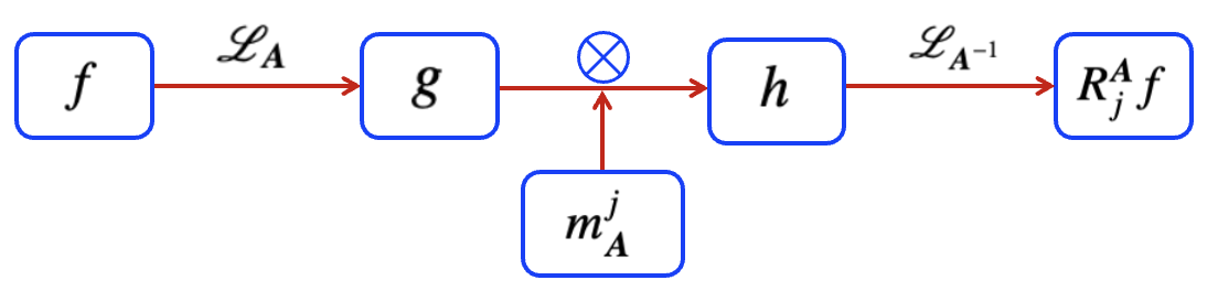
Figure 2: The decomposition of the $j$th LCRT $R_{j}^{\boldsymbol{A}}f$.

Next, we establish the boundedness of the LCRT on Lebesgue spaces.

Theorem 2.10.

Let $k,j\in\{1,\ldots,n\}$ and $\boldsymbol{A}:=(A_{1},\ldots,A_{n})$ with $A_{k}:=\begin{bmatrix}{a_{k}}&{b_{k}}\\ {c_{k}}&{d_{k}}\end{bmatrix}\in{M_{2\times 2}}(\mathbb{R})$ and both $b_{k}\neq 0$ and $a_{k}=d_{k}$ for all $k$. For any give $p\in(1,\infty)$, $R_{j}^{\boldsymbol{A}}$ can be extended to a linear bounded operator on $L^{p}(\mathbb{R}^{n})$ and, moreover, there exists a positive constant $C$ such that, for any $f\in L^{p}(\mathbb{R}^{n})$, $\|R_{j}^{\boldsymbol{A}}(f)\|_{L^{p}(\mathbb{R}^{n})}\leq C\|f\|_{L^{p}(\mathbb{R}^{n})}.$

Proof.

We first assume $f\in\mathscr{S}(\mathbb{R}^{n})$. By the integral definitions [see Definition 2.5 and Remark 2.6(i)] of both the Riesz transform and the LCRT, we obtain, for any $\boldsymbol{x}\in{\mathbb{R}^{n}}$, $R_{j}^{\boldsymbol{A}}(f)(\boldsymbol{x})={e}_{\boldsymbol{b},-\boldsymbol{d}}(\boldsymbol{x})R_{j}({e}_{\boldsymbol{b},\boldsymbol{a}}f)(\boldsymbol{x}),$ where ${e}_{\boldsymbol{b},-\boldsymbol{d}}$ is the same as in (1.1) with $\boldsymbol{a}$ and $\boldsymbol{b}$ replaced, respectively, by ${\boldsymbol{b}}$ and ${-\boldsymbol{d}}$, ${e}_{\boldsymbol{b},\boldsymbol{a}}$ is the same as in (1.1) with exchanging the position of $\boldsymbol{a}$ and $\boldsymbol{b}$, and $R_{j}$ is the same as in Remark 2.6(i). Using this and the boundedness of the classical Riesz transform on $L^{p}(\mathbb{R}^{n})$ (see, for example, [24, Corollary 5.2.8]), we immediately obtain the boundedness of the LCRT $R_{j}^{\boldsymbol{A}}$ on $L^{p}(\mathbb{R}^{n})\cap\mathscr{S}(\mathbb{R}^{n})$.

Now, let $p\in(1,\infty)$ and $f\in L^{p}(\mathbb{R}^{n})$. Since $\mathscr{S}(\mathbb{R}^{n})$ is dense in $L^{p}(\mathbb{R}^{n})$ (see, for example, [51, p. 20]), we deduce that there exists a sequence $\{g_{l}\}_{l\in\mathbb{N}}$ in $\mathscr{S}(\mathbb{R}^{n})$ such that $g_{l}\to f$ in $L^{p}(\mathbb{R}^{n})$ as $l\to\infty$. Thus, $\{g_{l}\}_{l\in\mathbb{N}}$ is a Cauchy sequence in $L^{p}(\mathbb{R}^{n})$. Note that $\{{e}_{\boldsymbol{b},\boldsymbol{a}}g_{l}\}_{l\in\mathbb{N}}$ is still a sequence in $\mathscr{S}(\mathbb{R}^{n})$ and, by the just proved boundedness of $R_{j}^{\boldsymbol{A}}$ on $L^{p}(\mathbb{R}^{n})\cap\mathscr{S}(\mathbb{R}^{n})$, we find that, for any $l,m\in\mathbb{N}$,

$$\left\|R_{j}^{\boldsymbol{A}}(g_{l})-R_{j}^{\boldsymbol{A}}(g_{m})\right\|_{L^{p}(\mathbb{R}^{n})}\lesssim\left\|g_{l}-g_{m}\right\|_{L^{p}(\mathbb{R}^{n})},$$

which further implies that $\{R_{j}^{\boldsymbol{A}}(g_{l})\}_{l\in\mathbb{N}}$ is also a Cauchy sequence in $L^{p}(\mathbb{R}^{n})$. From this and the completeness of $L^{p}(\mathbb{R}^{n})$, we infer that $\lim_{l\to\infty}R_{j}^{\boldsymbol{A}}(g_{l})$ exists in $L^{p}(\mathbb{R}^{n})$. Let $R_{j}^{\boldsymbol{A}}(f):=\lim_{l\to\infty}R_{j}^{\boldsymbol{A}}(g_{l})$ in $L^{p}(\mathbb{R}^{n})$. Then it is easy to show that $R_{j}^{\boldsymbol{A}}(f)$ is independent of the choice of $\{g_{l}\}_{l\in\mathbb{N}}$ and hence is well-defined. Moreover, by the Minkowski norm inequality of $L^{p}(\mathbb{R}^{n})$ and the just proved boundedness of $R_{j}^{\boldsymbol{A}}$ on $L^{p}(\mathbb{R}^{n})\cap\mathscr{S}(\mathbb{R}^{n})$ again, we obtain

$$\left\|R_{j}^{\boldsymbol{A}}(f)\right\|_{L^{p}(\mathbb{R}^{n})}=\lim_{l\to\infty}\left\|R_{j}^{\boldsymbol{A}}(g_{l})\right\|_{L^{p}(\mathbb{R}^{n})}\lesssim\lim_{l\to\infty}\|g_{l}\|_{L^{p}(\mathbb{R}^{n})}=\|f\|_{L^{p}(\mathbb{R}^{n})},$$

which then completes the proof of Theorem 2.10. ∎

3 Numerical Simulations

In this section, we perform LCRTs numerical simulations of images by using the discrete LCT algorithm and the LCRT multiplier (see, for example, the inspiring comprehensive monograph [47] for similar numerical simulations). Due to the fast algorithm of LCTs, the complexity of this algorithm is significantly reduced compared with the convolution type LCRT. Through a series of simulation experiments, we successfully demonstrate that LCRTs not only have the effect of shifting terms, but can also attenuate the amplitude in the LCT domain. Furthermore, we conduct numerical simulations of images by using LCHTs and conduct a complete comparison of the numerical results between LCRTs and LCHTs, clarifying the distinctions between them. This comparison not only deepens our understanding of these two transforms, but also lays the foundation for their further applications in signal processing, thereby opening doors to new application directions.

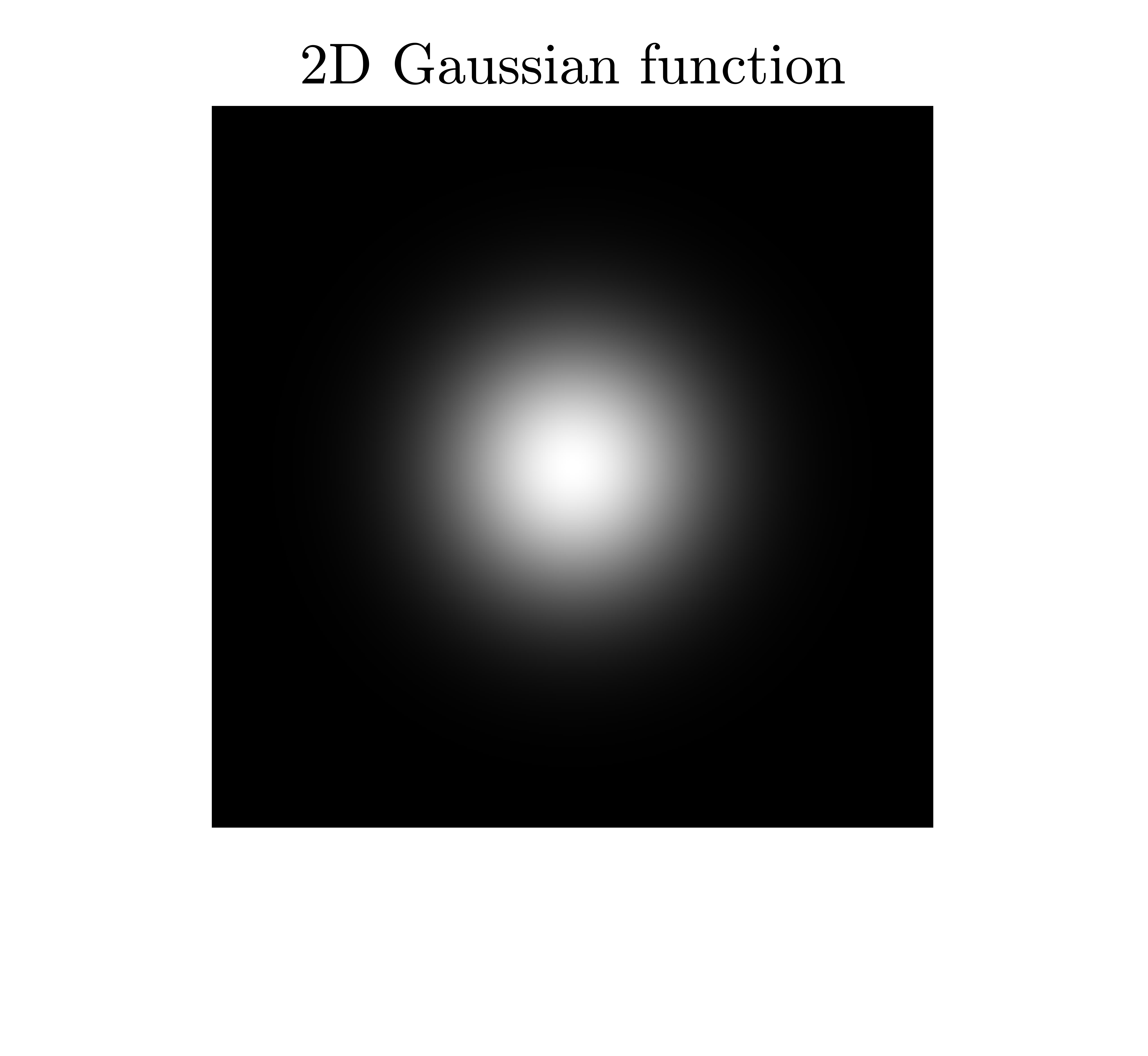
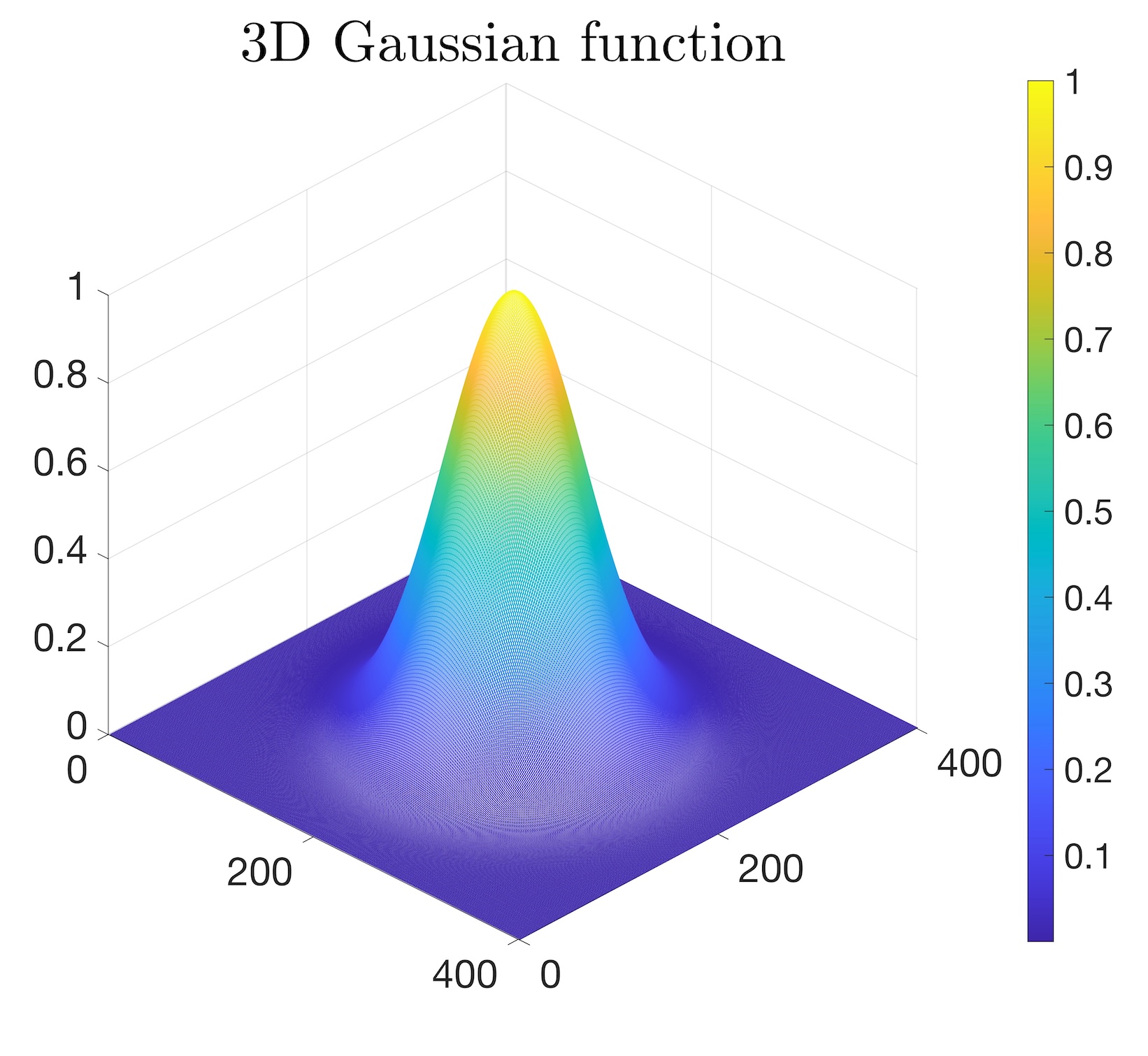
Figure 3: Gaussian function as a test image.

Graphs (a) and (b) in Figure 3 are the test images used for numerical simulations in this whole section. Graph (a) presents a $400\times 400$ pixel 2D grayscale image, while Graph (b) is a three-dimensional (for short, 3D) color image of Graph (a). In the continuous case, Graph (a) can be represented by the following Gaussian function $G$, which is defined by setting, for any $(x_{1},x_{2})\in[0,400]^{2}$,

$$G(x_{1},x_{2}):=e^{-\frac{(x_{1}-200)^{2}+(x_{2}-200)^{2}}{2\cdot\sigma^{2}}},$$

where $x_{1}$ and $x_{2}$ are the coordinates in the image matrix and $\sigma$ is the standard deviation, with $\sigma=50$. The center of Graph (a) is located at $(200,200)$. Finally, the pixel values of Graph (a) are normalized to ensure that its image data falls within the range of $0$ to $1$, which is a common practice to maintain consistency during display or further processing.

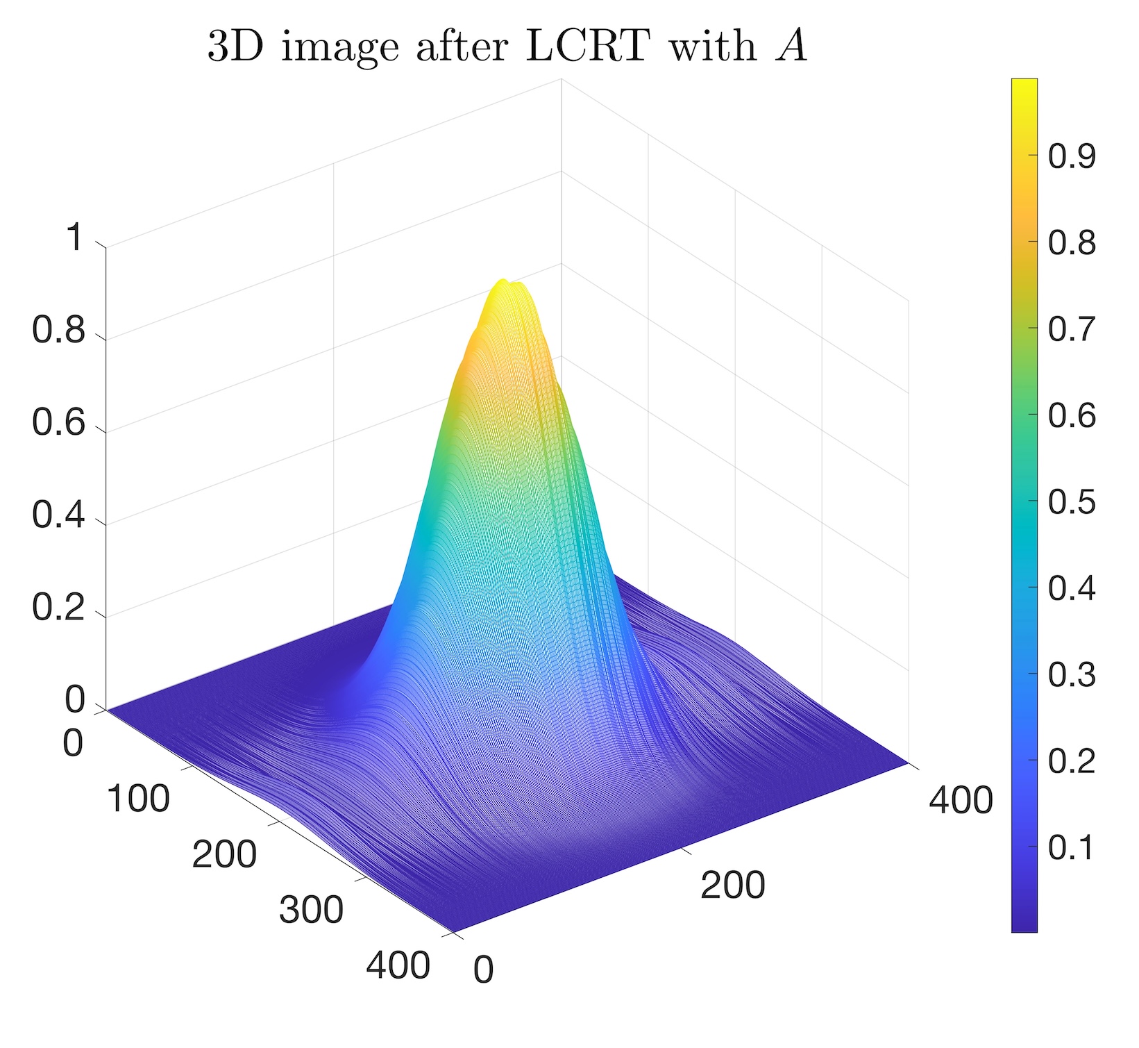
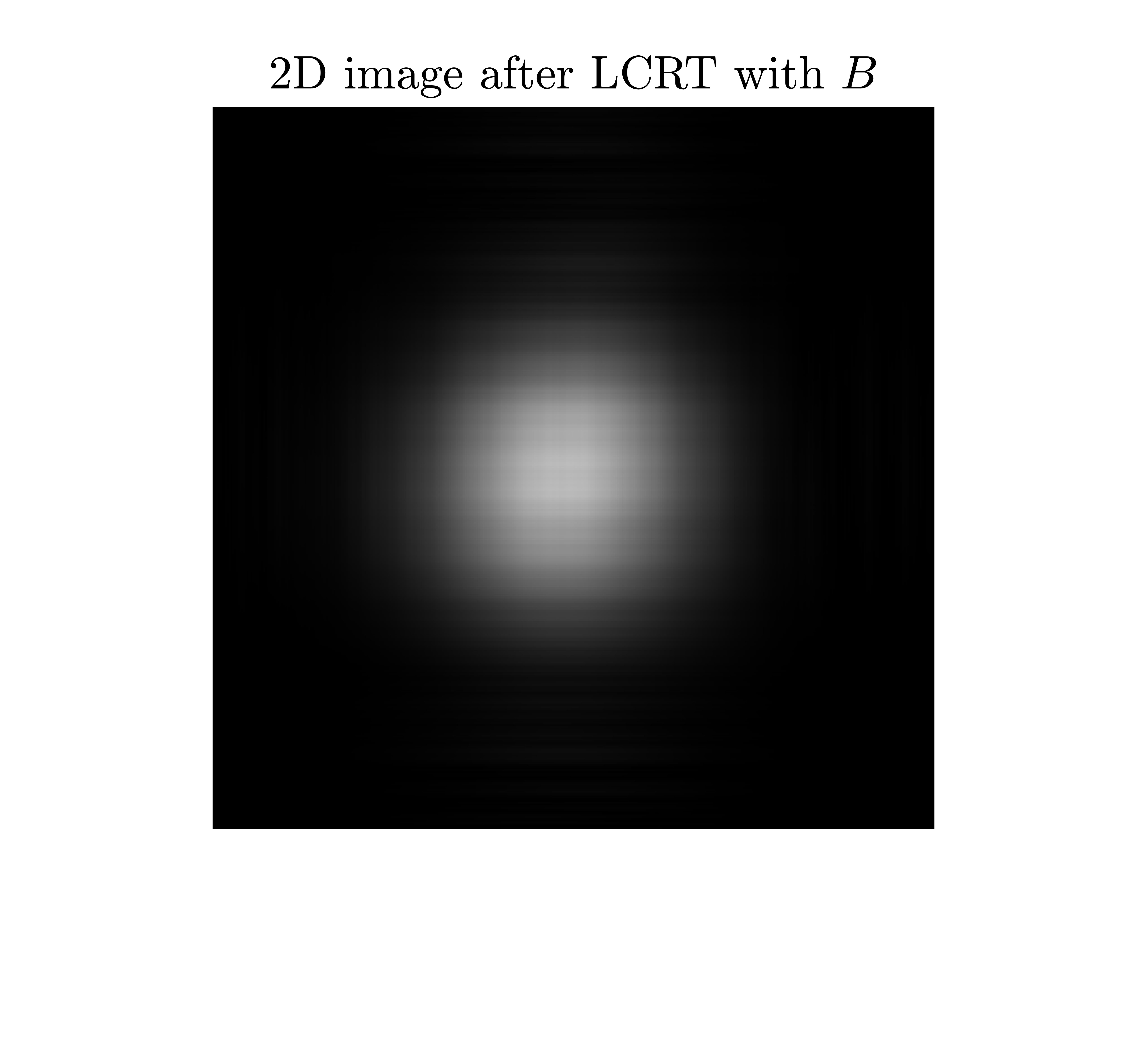
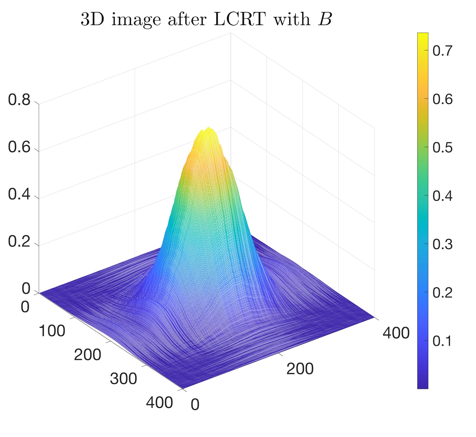
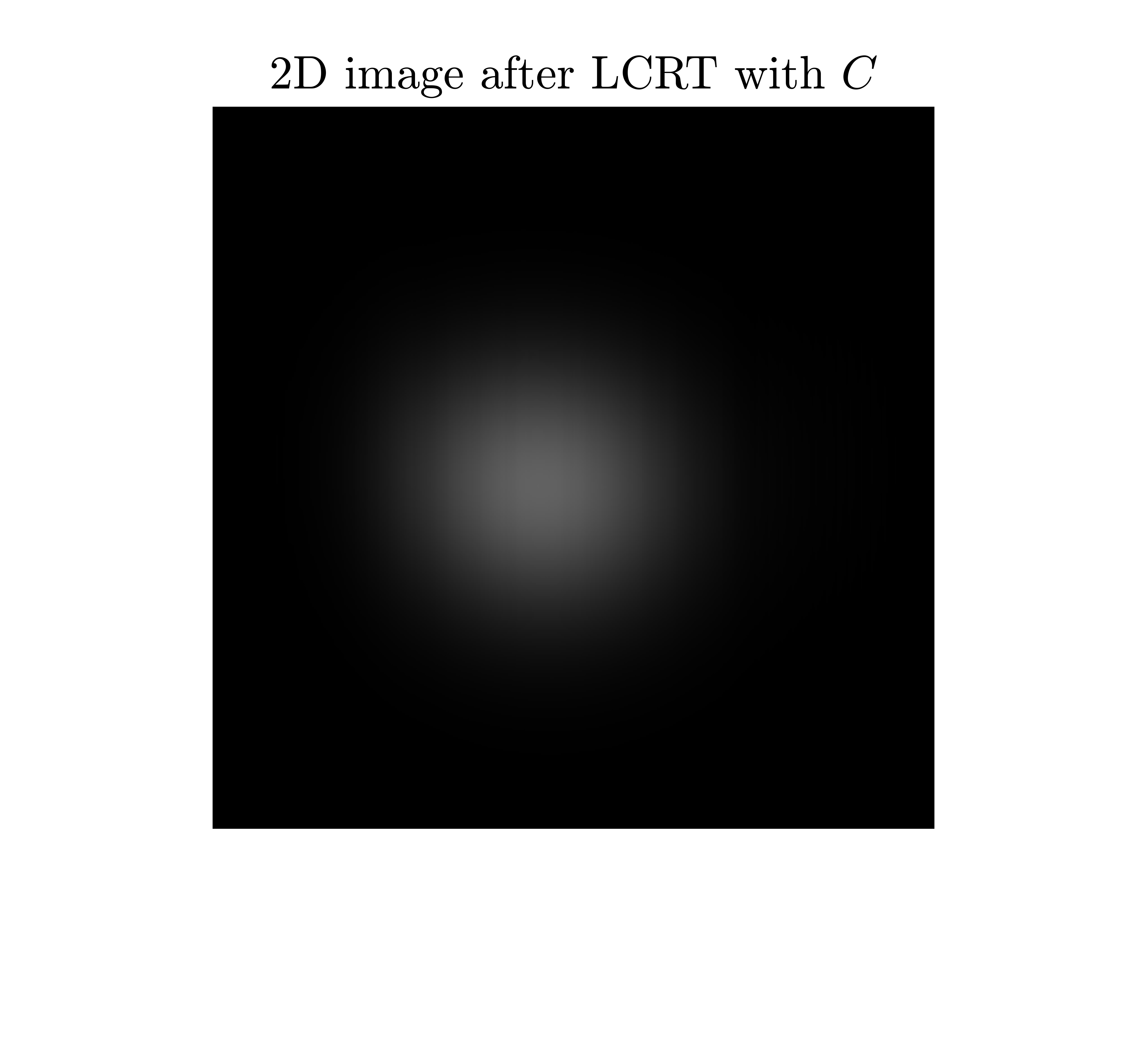
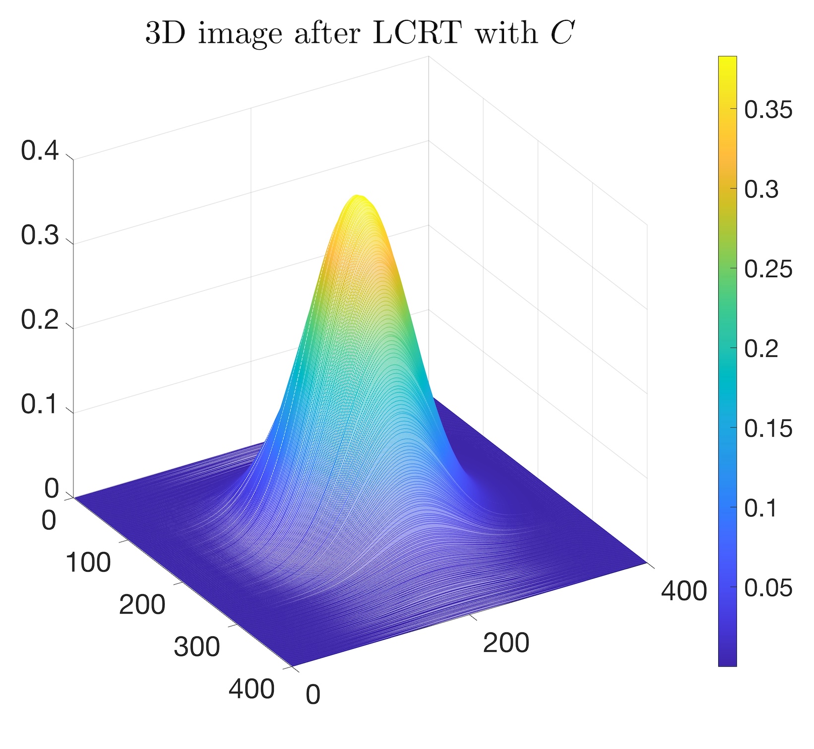
Figure 4: 2D and 3D images of the test image after applying LCRT with different parameters are shown. Graphs (a) and (b), (c) and (d), and (d) and (e) correspond to LCRT parameters ${\boldsymbol{A}}$, ${\boldsymbol{B}}$, and ${\boldsymbol{C}}$, respectively.

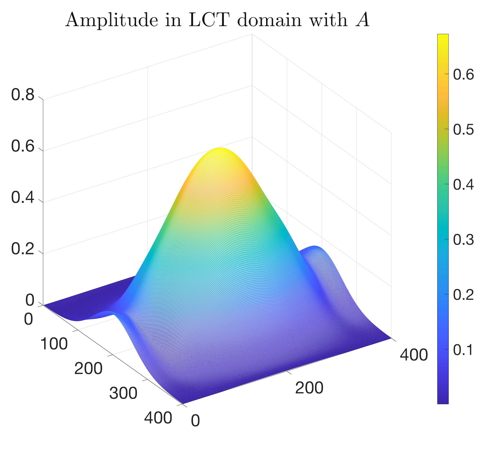
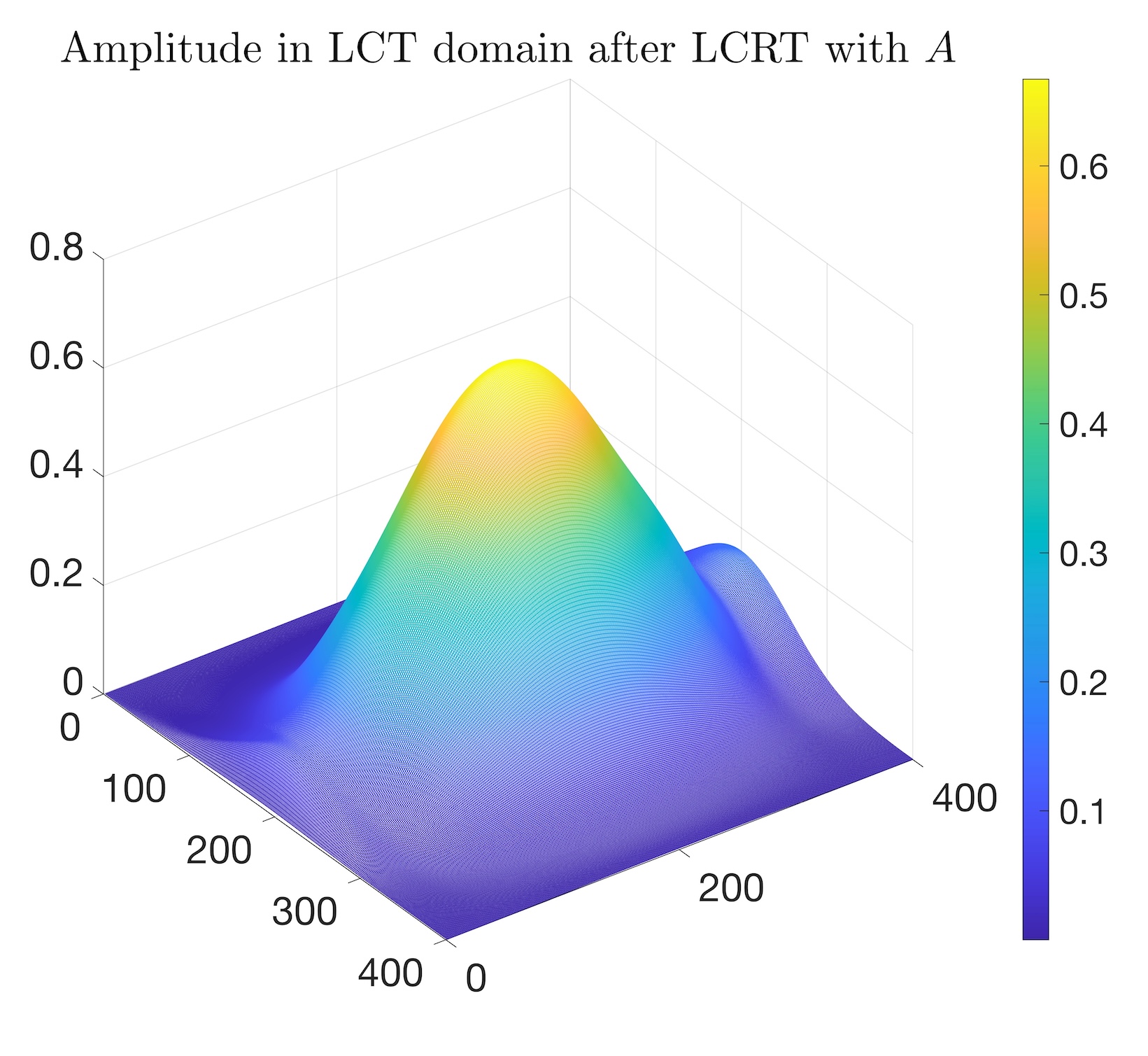
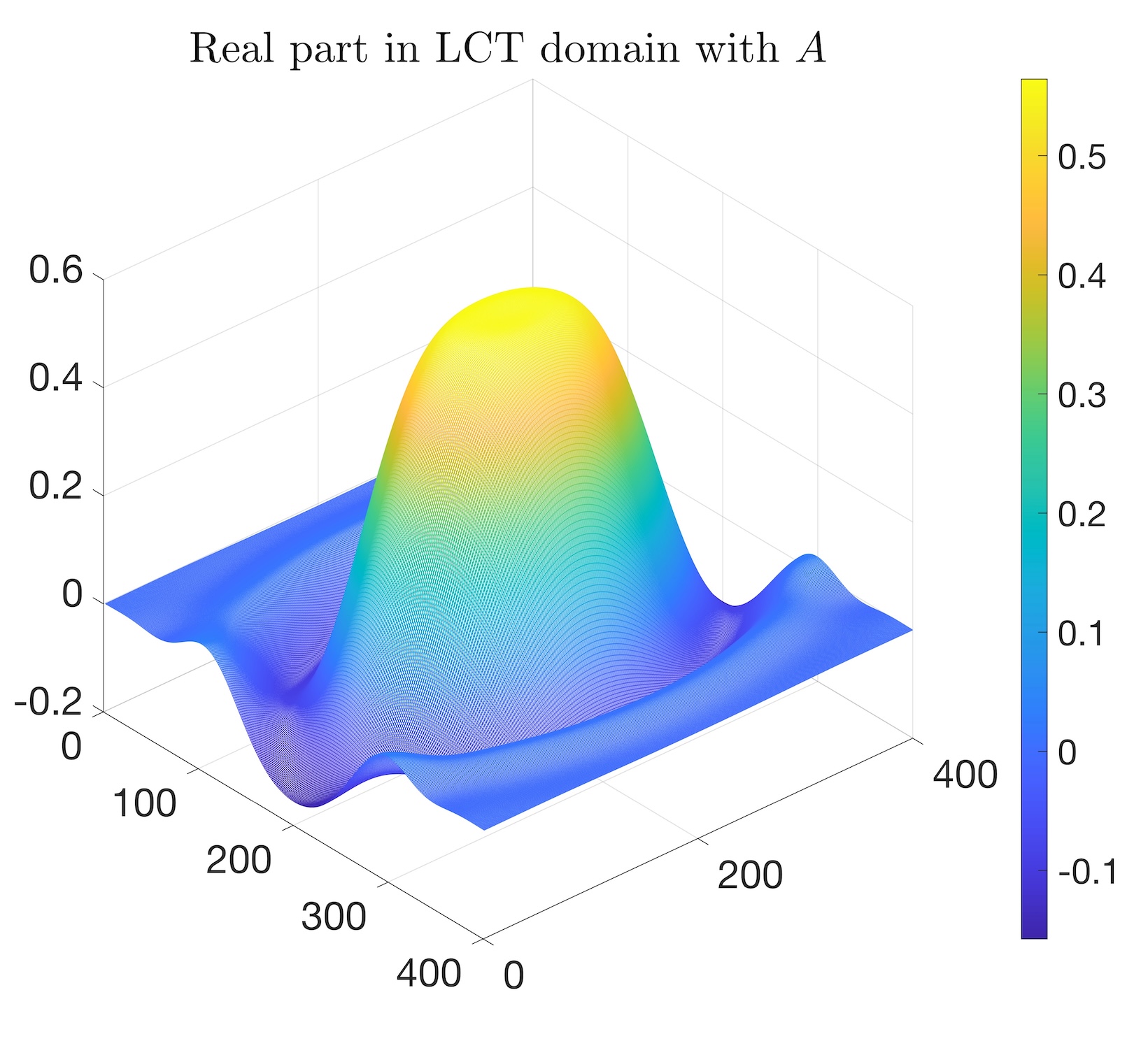
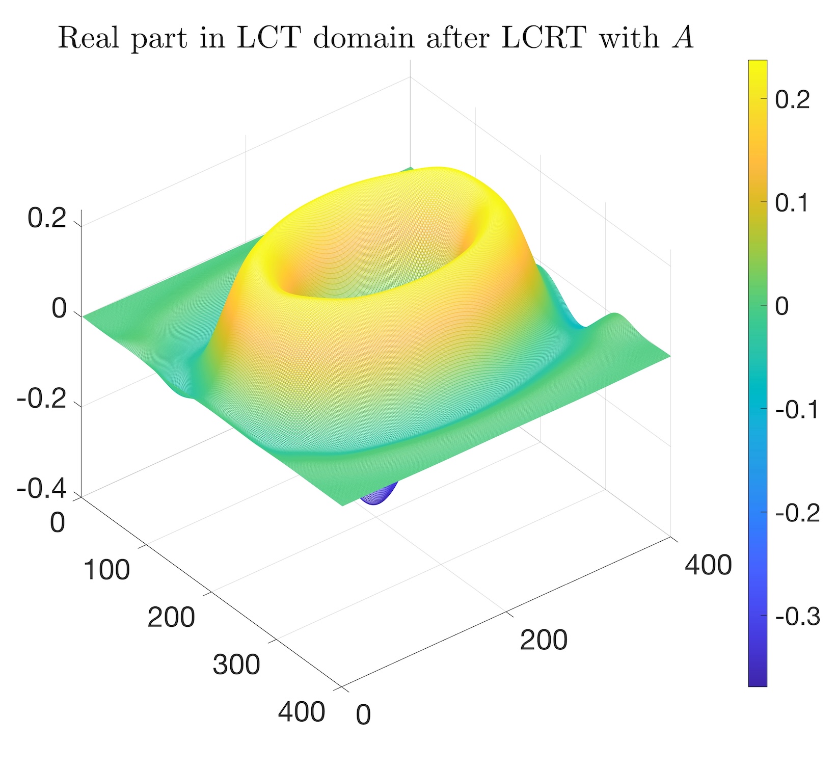
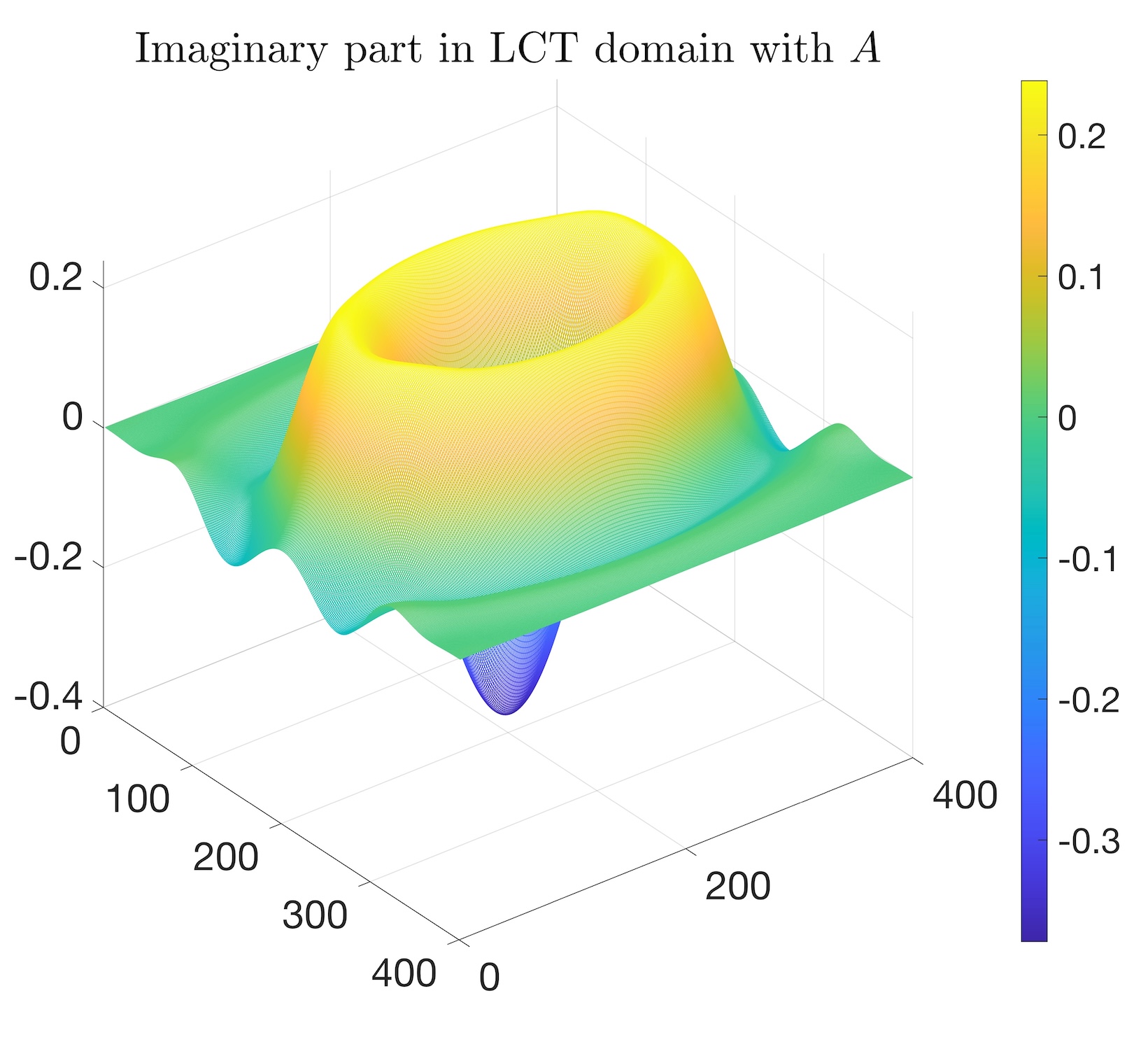
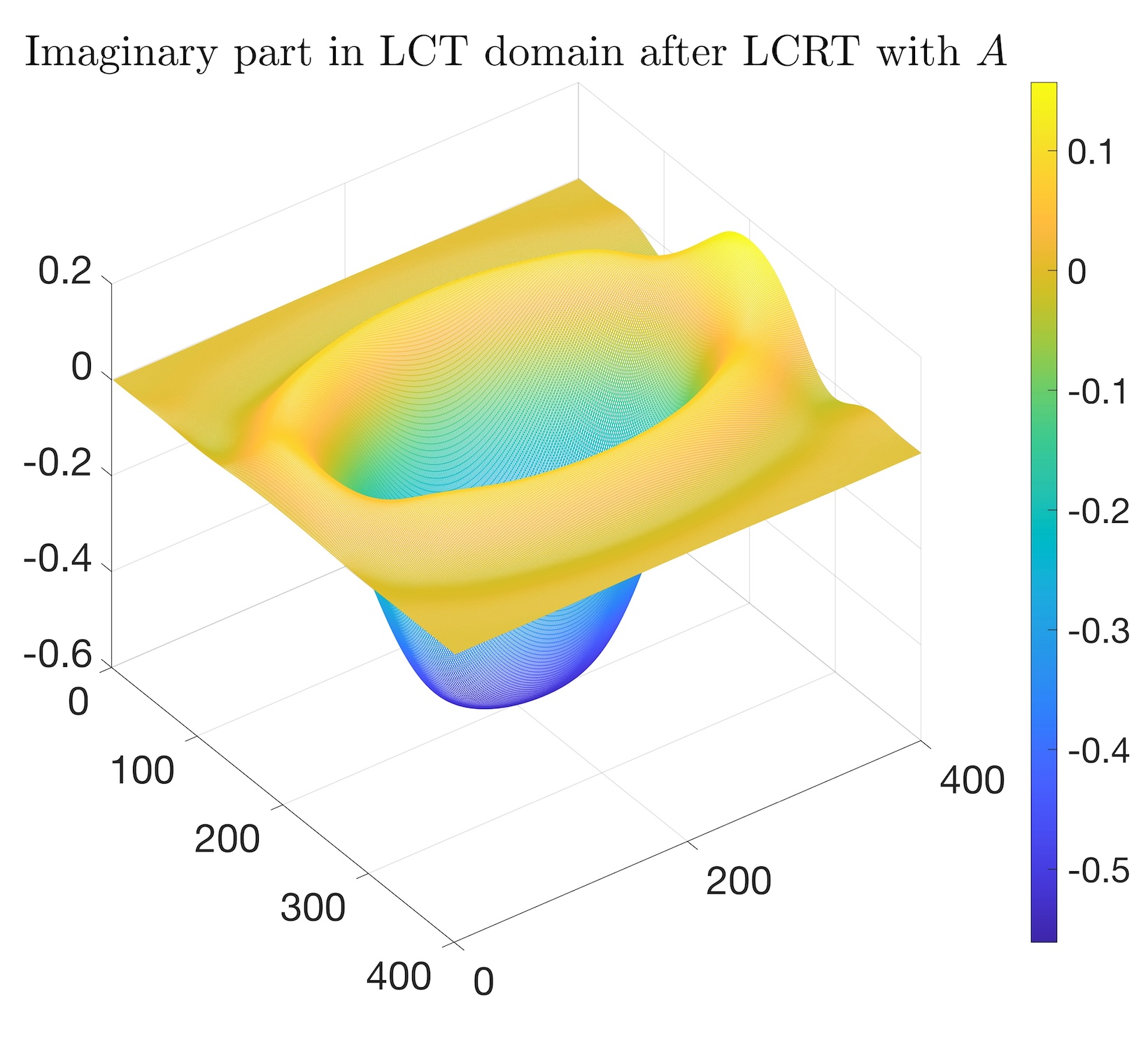
Figure 5: The amplitude, the real part, and the imaginary part of the original test image in the LCT domain, and those of the original image after applying LCRTs in the LCT domain with the corresponding parameter ${\boldsymbol{A}}$.

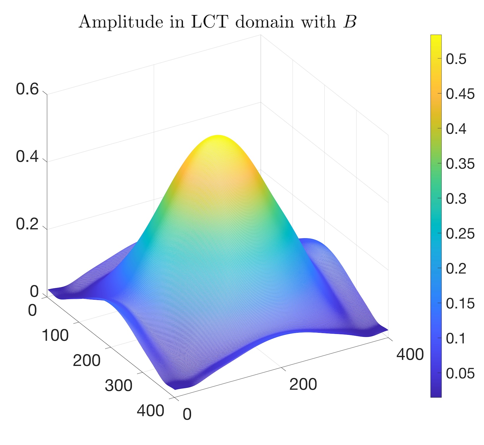
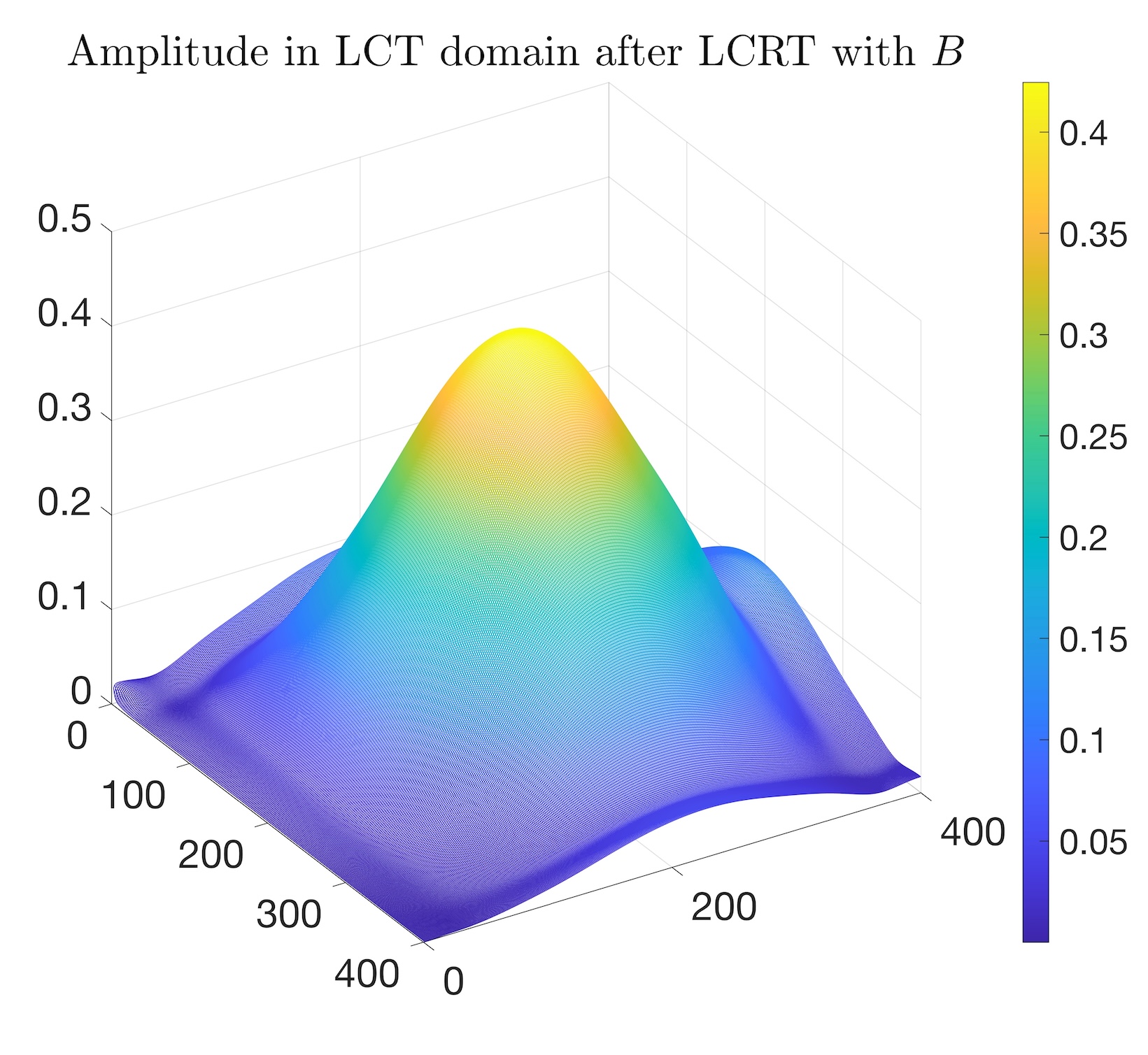
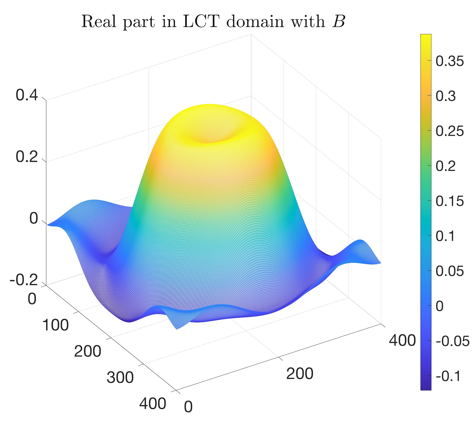
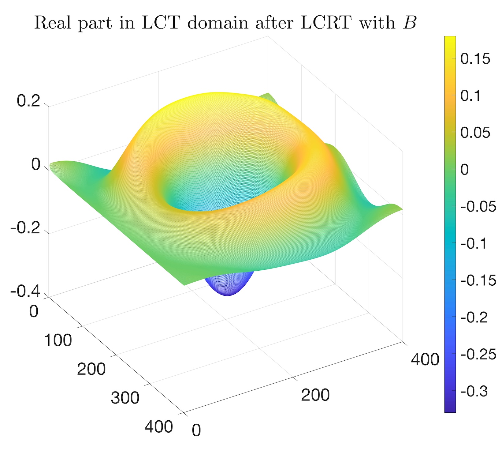
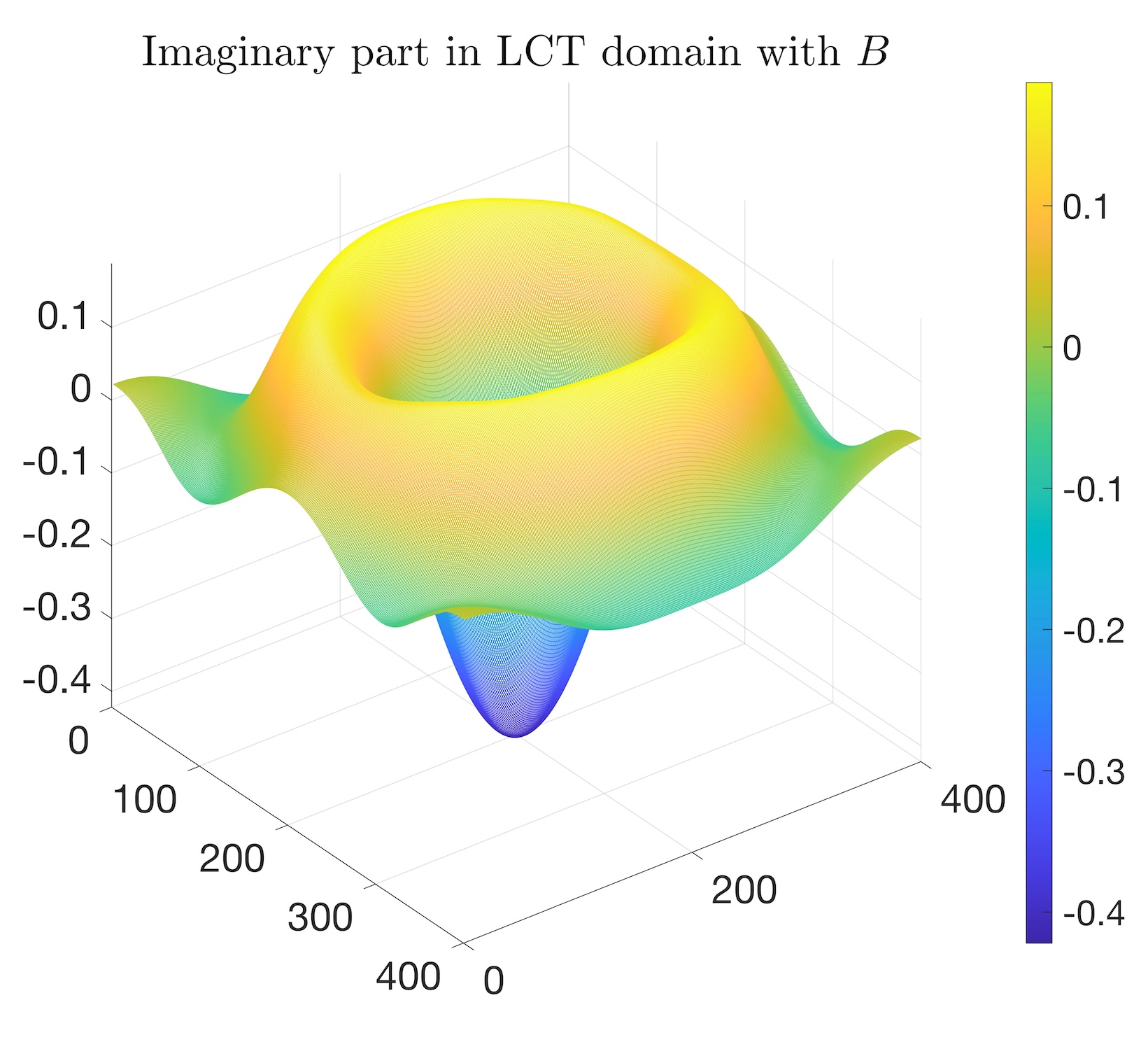
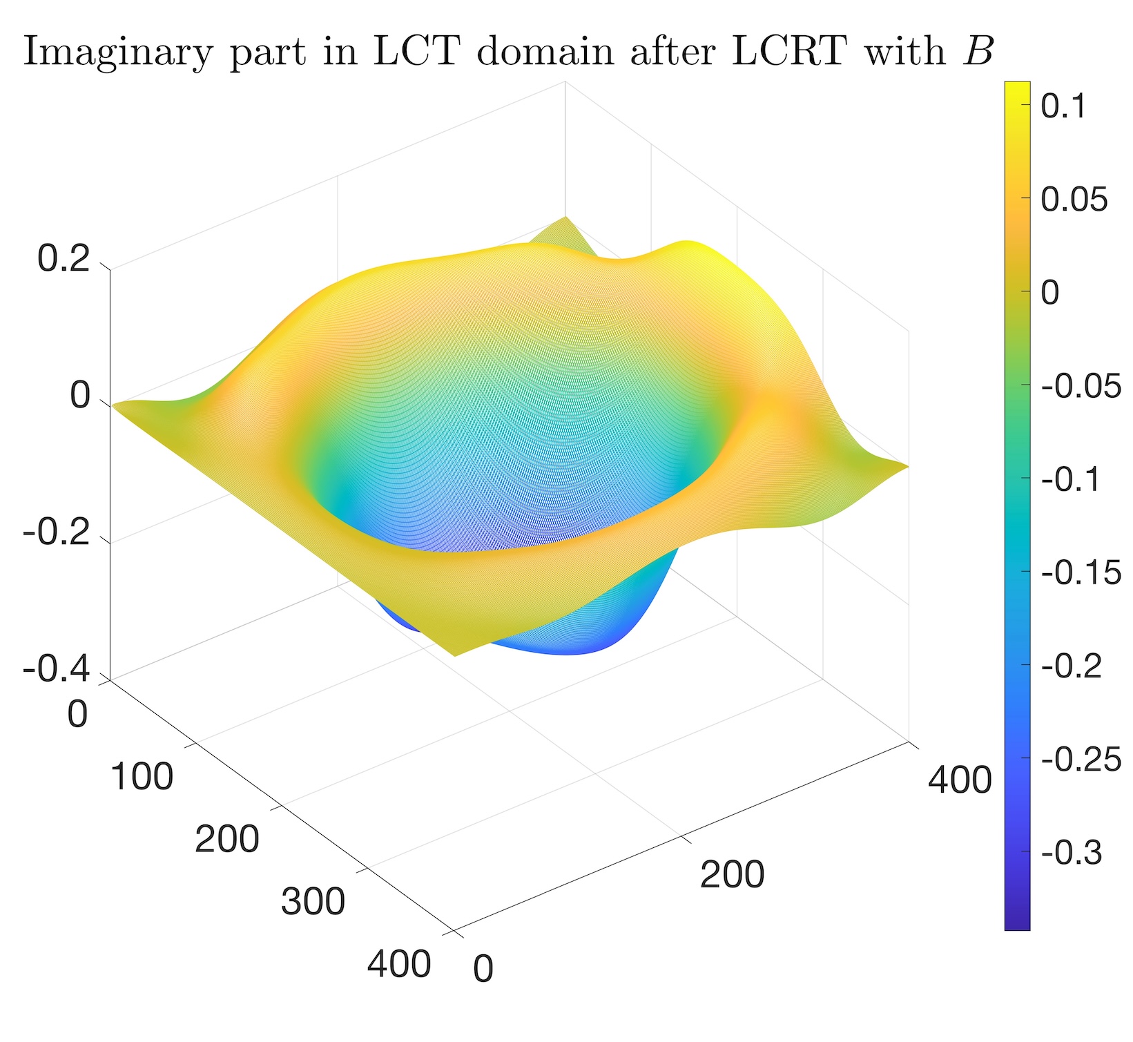
Figure 6: The amplitude, the real part, and the imaginary part of the original test image in the LCT domain, and those of the original image after applying LCRTs in the LCT domain with the corresponding parameter ${\boldsymbol{B}}$.

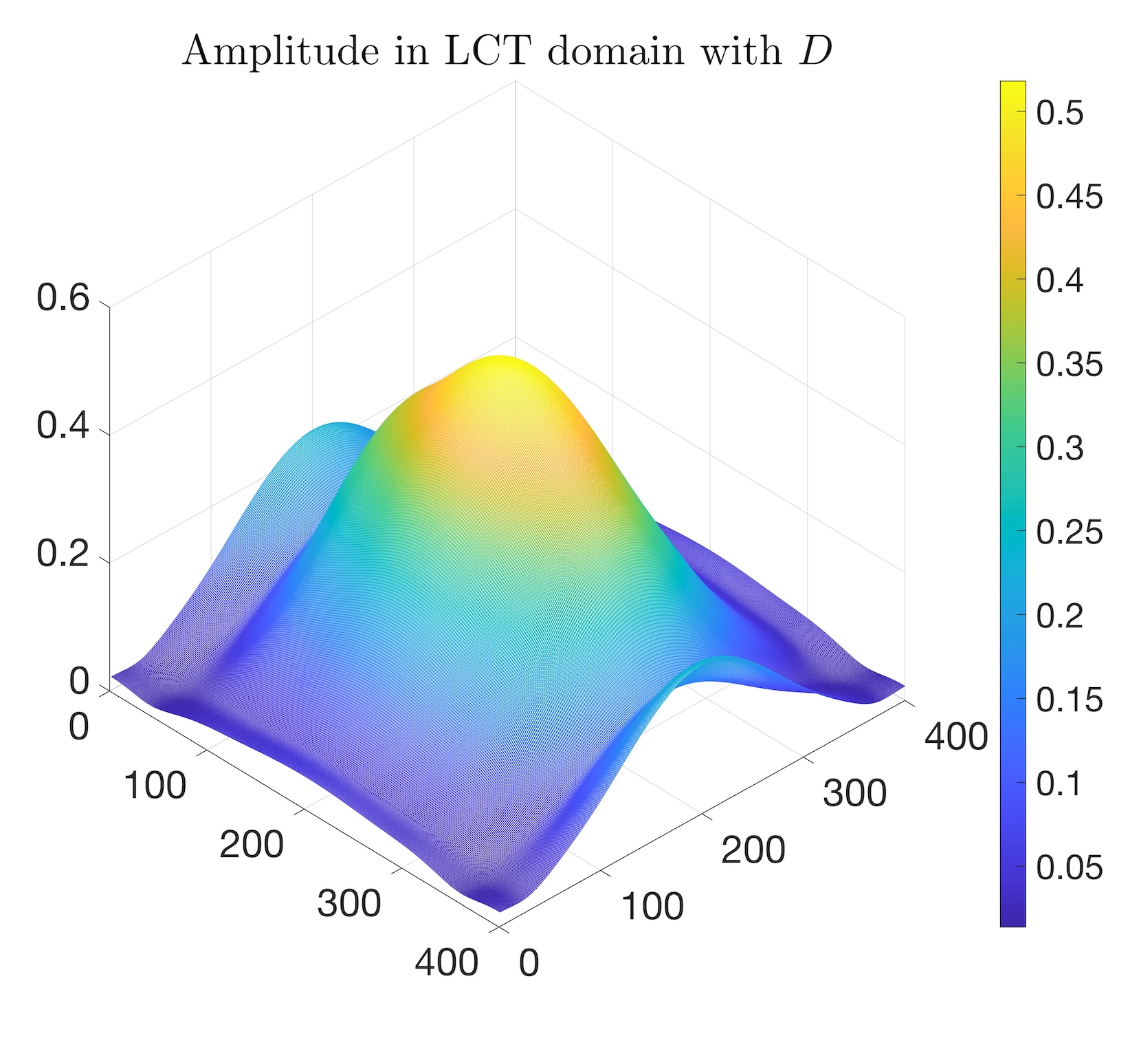
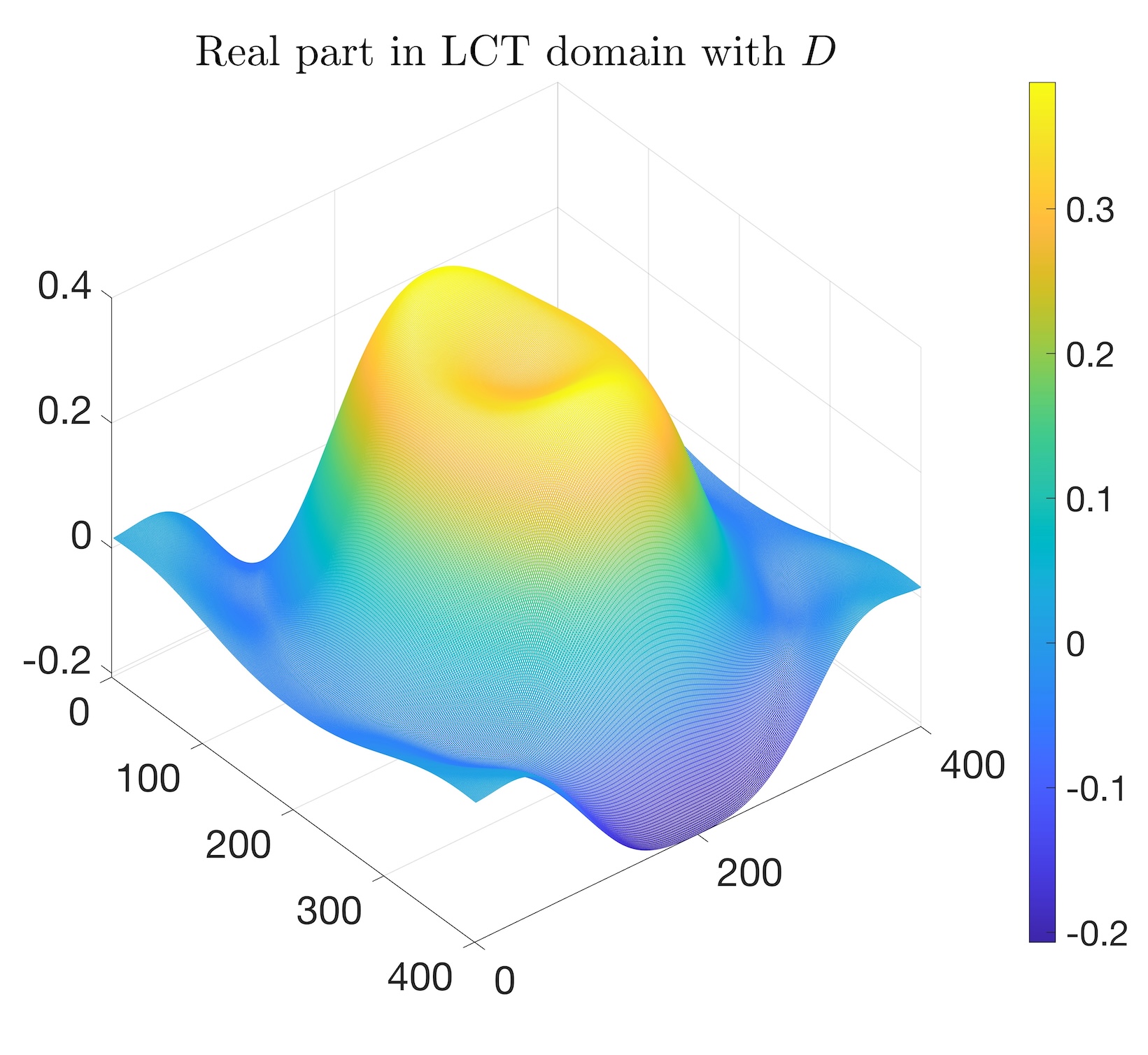
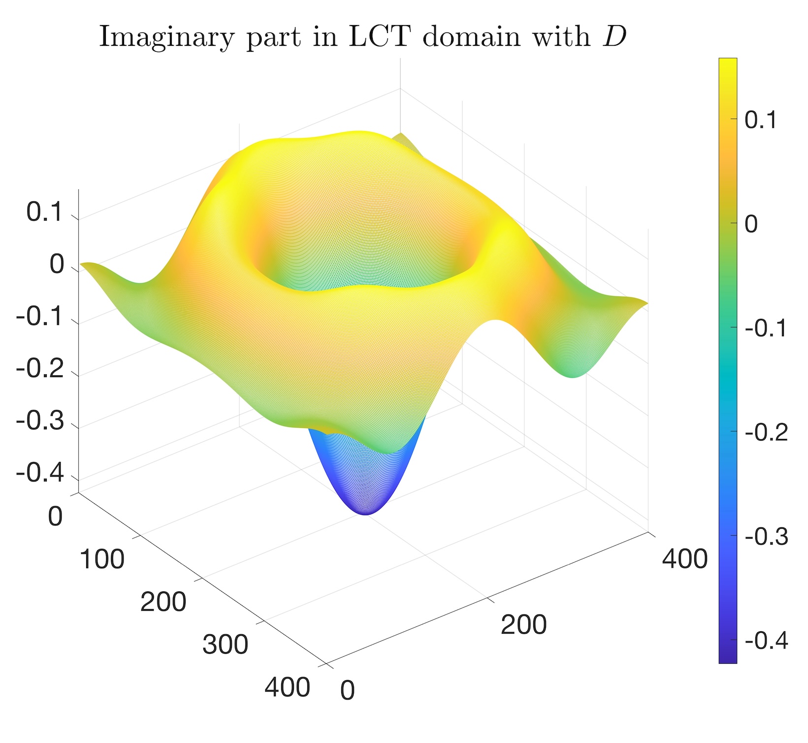
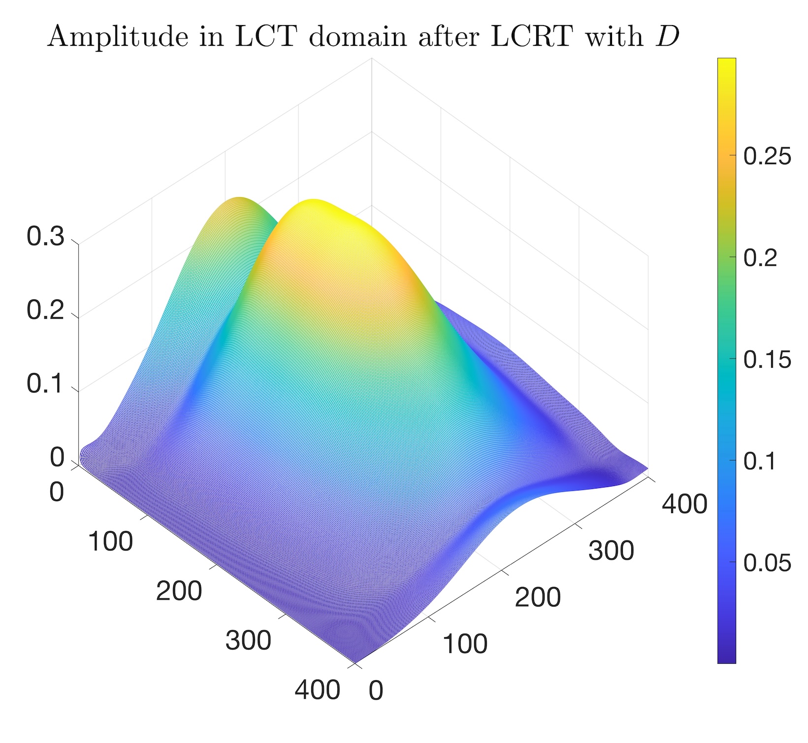
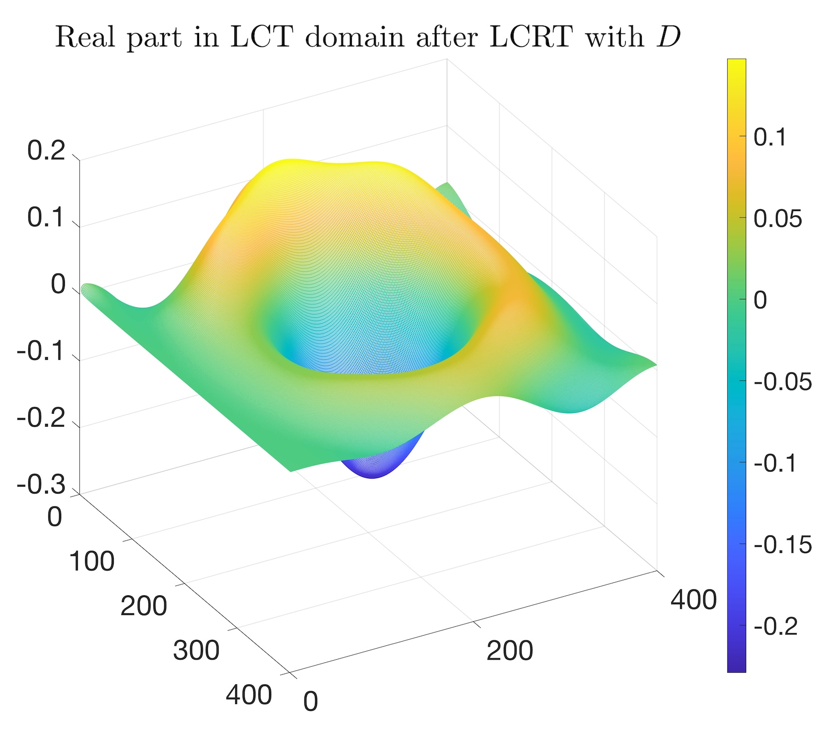
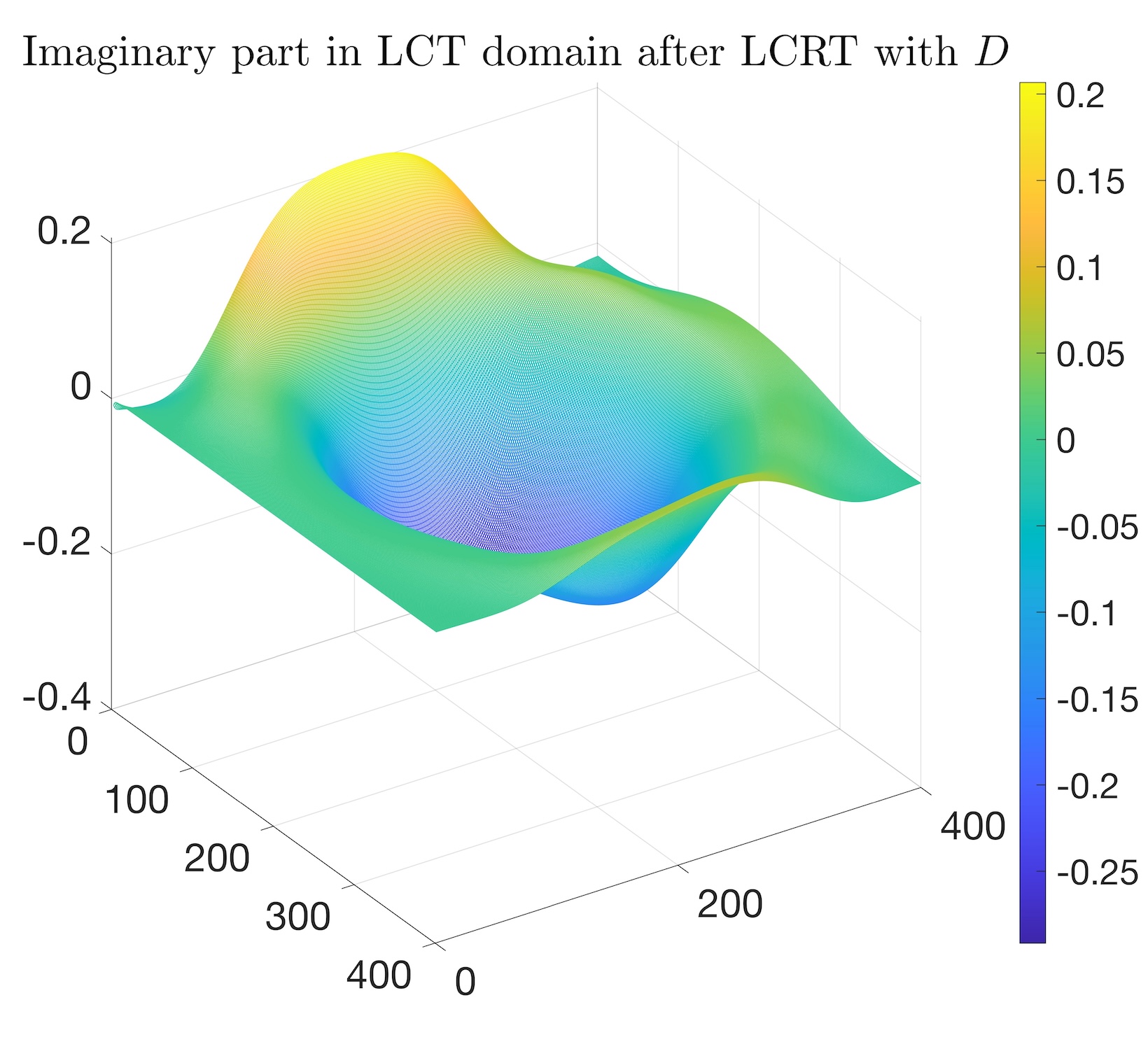
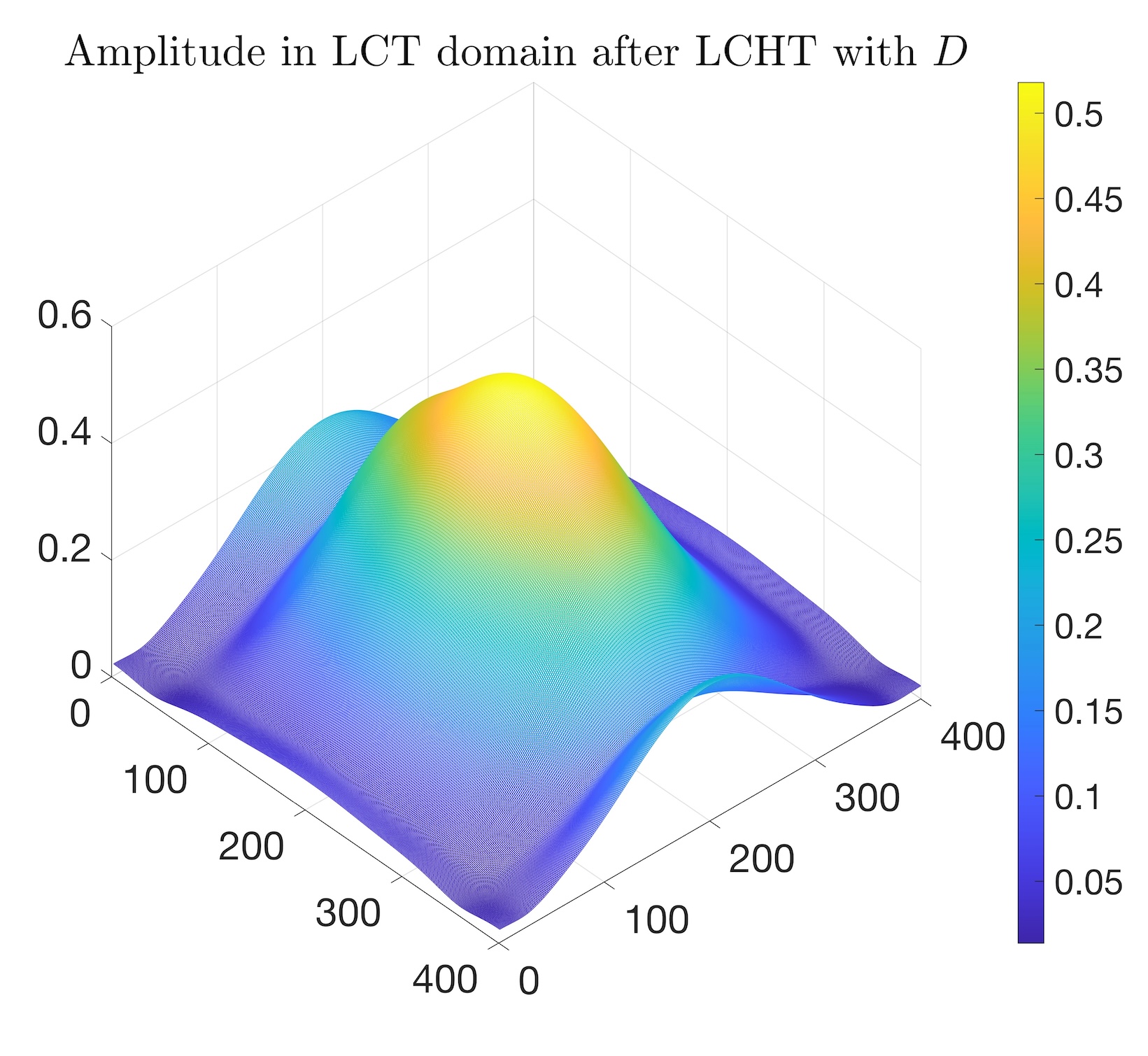
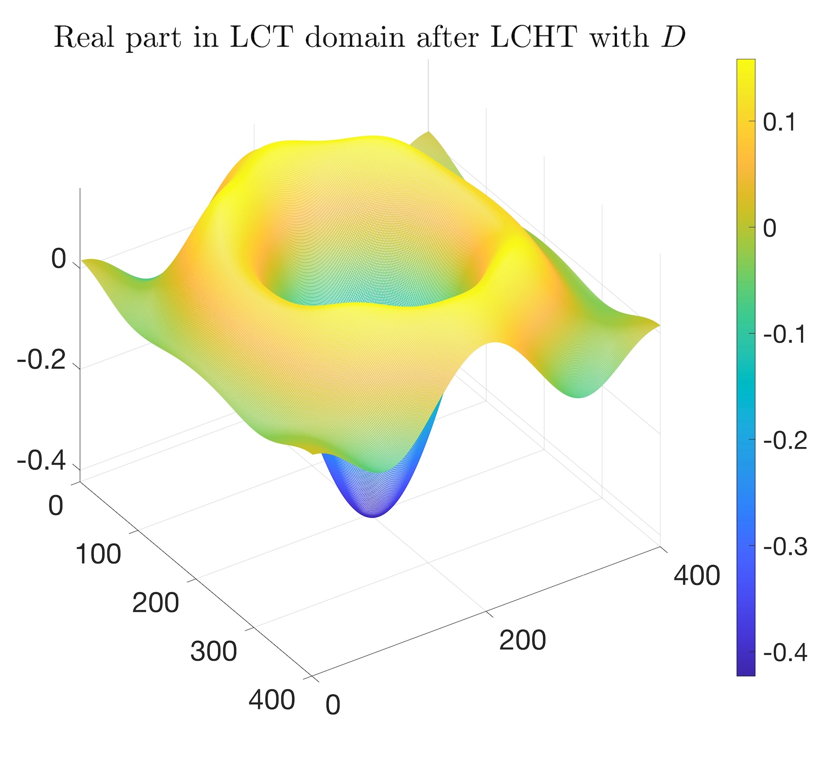
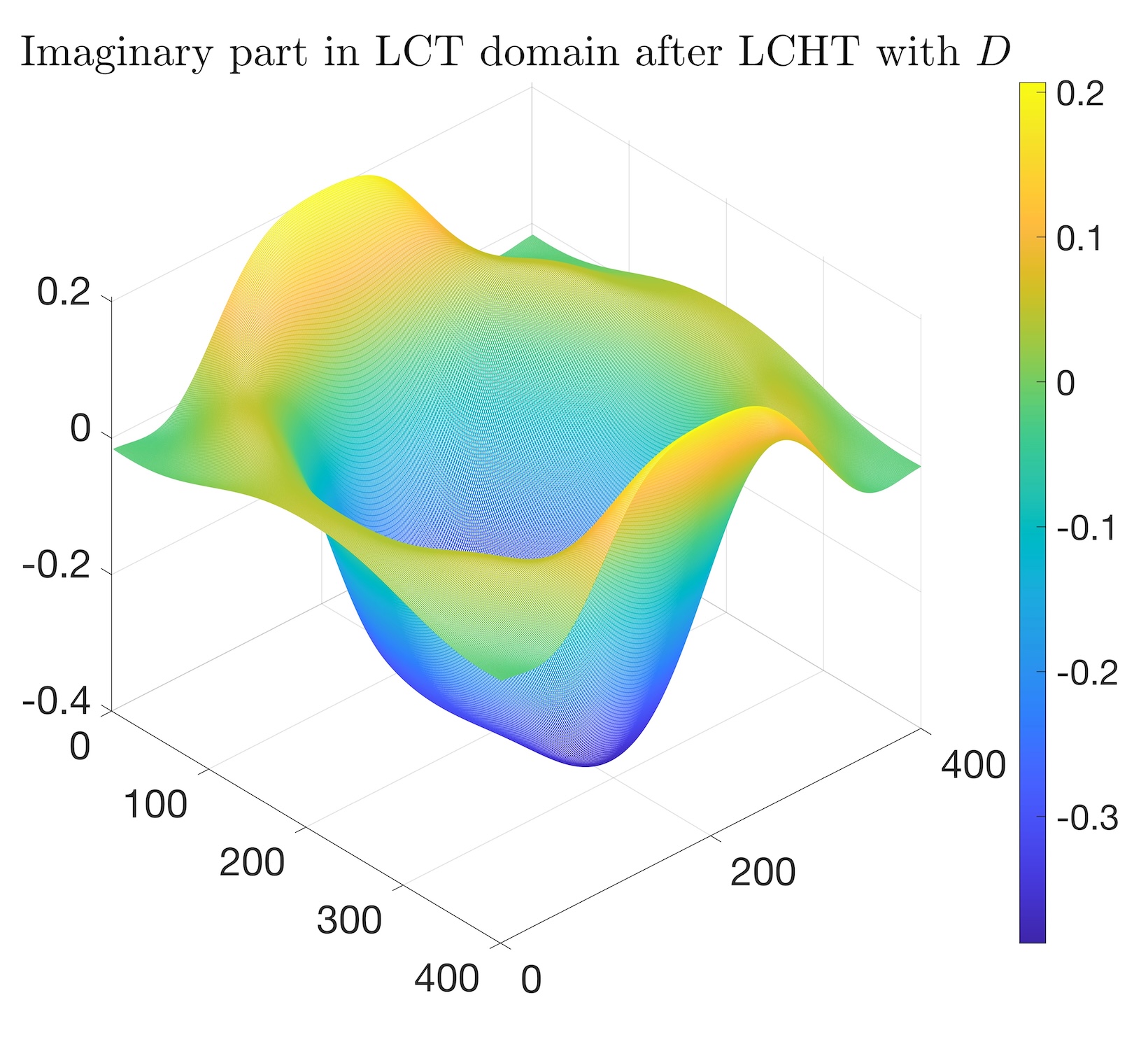
Figure 7: In the LCT domain, the amplitude, the real part, as well as the imaginary part of the original test image, and those of the original image after applying LCRTs and HLCHTs, are presented, with the corresponding parameter being ${\boldsymbol{D}}$.

In Figure 4, Graphs (a), (c), and (e) represent grayscale images obtained by applying LCRTs $R_{1}^{\boldsymbol{A}}$, $R_{1}^{\boldsymbol{B}}$, and $R_{1}^{\boldsymbol{C}}$ with different parameters on Graph (a) in Figure 3. Their parameter matrices correspond, respectively, to ${\boldsymbol{A}}:=(A_{1},A_{2})$ with $A_{1}:=\begin{bmatrix}{6}\ &{50}\\ {0.7}\ &{6}\end{bmatrix}$ and $A_{2}:=\begin{bmatrix}{3}\ &{400}\\ {0.02}\ &{3}\end{bmatrix}$, ${\boldsymbol{B}}:=(B_{1},A_{2})$ with $B_{1}:=\begin{bmatrix}{10}\ &{330}\\ {0.3}\ &{10}\end{bmatrix}$, and ${\boldsymbol{C}}:=(C_{1},C_{2})$ with $C_{1}:=\begin{bmatrix}{20}\ &{39.9}\\ {10}\ &{20}\end{bmatrix}$ and $C_{2}:=\begin{bmatrix}{4}\ &{1}\\ {15}\ &{4}\end{bmatrix}$. Also, in Figure 4, Graphs (b), (d), and (f) show the 3D color images of Graphs (a), (c), and (e), respectively. From Figure 4, we infer that applying LCRTs with different parameter matrices to the same test image yields significantly different effects, which further indicates that parameter matrices of LCRTs completely determine its role.

In Figure 5, Graphs (a), (c), and (e) represent, respectively, the amplitude, the real part, and the imaginary part of the original test image in Figure 3 in the LCT domain, while Graphs (b), (d), and (f) represent, respectively, the amplitude, the real part, and the imaginary part of the original test image in Figure 3 after applying LCRTs in the LCT domain using the same parameter matrix ${\boldsymbol{A}}$ as in Figure 4. Comparing Graphs (a) with (b), we find that LCRTs dramatically attenuate the amplitude in the LCT domain. Additionally, by comparing Graphs (c) with (f) and Graphs (e) with (d), we find that LCRTs have an obvious shifting effect in the LCT domain.

Replacing the parameter matrix ${\boldsymbol{A}}$ with the parameter matrix ${\boldsymbol{B}}$ (both ${\boldsymbol{A}}$ and ${\boldsymbol{B}}$ are the same as in Figure 4) and then repeating the experiment same as in Figure 5, we obtain Figure 6. We find that, in different LCT domains, LCRTs always have obvious and different effects of shifting and amplitude attenuation. Therefore, it is important to select the appropriate LCT domain for solving various problems.

In Figure 7, we compare the amplitude, the real part, and the imaginary part of the original test image in Figure 3, the original test image in Figure 3 after applying LCRTs $R_{1}^{\boldsymbol{D}}$, and the original test image in Figure 3 after applying HLCHTs $H_{x}^{D_{1}}$ in the LCT domain, where the corresponding parameter matrix is ${\boldsymbol{D}}:=(D_{1},D_{2})$, where $D_{1}:=\begin{bmatrix}{6}\ &{500}\\ {0.07}\ &{6}\end{bmatrix}$ and $D_{2}:=\begin{bmatrix}{4}\ &{300}\\ {0.05}\ &{4}\end{bmatrix}$. Graphs (a), (d), and (g) represent the amplitude for the aforementioned three cases, while Graphs (b), (e), and (h) represent their real parts, and Graphs (c), (f), and (i) represent their imaginary parts. Observing Graphs (a), (d), and (g), we conclude that LCRTs have the effect of reducing amplitude in the LCT domain, whereas the HLCHT does not exhibit this effect. Comparing Graphs (b), (e), (h), (c), (f), and (i), we find that LCRTs induce a phase shift of $\pi/2$ in the LCT domain, and HLCHTs also have the same effect.

In summary, through a series of image simulation experiments, we have verified that LCRTs are able to yield both shifting and attenuation of amplitudes in the LCT domain. Compared to the HLCHT, the LCRT is able to attenuate amplitudes in the LCT domain, which may enhance performance in image feature extraction, image quality enhancement, and texture analysis, while, compared to fractional Riesz transforms, LCRTs provide a broader selection of frequency domains and greater flexibility, potentially resulting in more precise extraction of local image feature information.

4 Applications

In this section, we present the application of LCRT to refining image edge detection. In Section 4.1, we introduce the concept of the sharpness $R^{\rm E}_{\rm sc}$ of the edge strength and continuity of images associated with the LCRT, and propose a new LCRT image edge detection method (namely LCRT-IED method) and provide its mathematical foundation. The experimental results demonstrate that this new LCRT-IED method is able to gradually control of the edge strength and continuity by subtly adjusting the parameter matrices of the LCRT. Meanwhile, in local edge feature extraction, the LCRT-IED method better preserves fine image edge details in some sub-regions. In Section 4.2, we further summarize the advantages and features of the LCRT-IED method in image processing.

4.1 Refining Image Edge Detection by Using $R^{\rm E}_{\rm sc}$

The image processing has long been a central focus in information sciences, playing a vital role in applied sciences and garnering significant attention (see, for example, [6, 22, 23, 29]). In image processing, edge detection is one of the key steps in understanding image content. It involves extracting important structural information from images, such as contours and textures, which is crucial for image analysis and computer vision tasks. While traditional edge detection methods, such as the Canny and Sobel edge detectors, perform well in certain scenarios, they often struggle with complex or noisy images (see, for example, [9, 14]). Recently, the Riesz transform has garnered attention as a novel edge detection technique due to its advantages in the analysis of multi-scale and directional analysis tasks. The Riesz transform can provide richer edge information compared to traditional methods, demonstrating its superior performance in image processing (see, for example, [19, 36]). Based on the theoretical foundations of Riesz transforms and fractional Riesz transforms, this section explore the application of LCRTs in edge detection. Through the whole section, we work on $\mathbb{R}^{2}$.

In image processing and computer vision, edge strength and continuity are two crucial attributes that are essential for image analysis and understanding. Edge strength refers to the prominence of an edge within an image, typically associated with the rate of strength change at the edge. Regions with high edge strength exhibit greater changes in image strength, indicating a more pronounced edge. Edge strength information plays a vital role in tasks, such as image segmentation, feature extraction, and object recognition. In some cases, edge strength can be used to differentiate among different types of edges, such as contour edges and texture edges. Edge continuity describes the coherence of an edge within an image. A continuous edge means that edge points are closely connected without interruptions. In image segmentation and object detection, edge continuity is a key feature. Continuous edges help to define object boundaries, leading to more accurate image segmentation and object recognition.

Felsberg and Sommer [17] introduced the monogenic signal in image processing, while Larkin et al. [37] introduced this signal in the optical context. For an image $f$, the monogenic signal $\left(p,q_{1},q_{2}\right)$ is defined as the combination of $f$ and its LCRTs as follows:

$$\left(p,q_{1},q_{2}\right):=\left(f,R_{1}^{\boldsymbol{A}}f,R_{2}^{\boldsymbol{A}}f\right),$$

where the LCRTs $R_{1}^{\boldsymbol{A}}$ and $R_{2}^{\boldsymbol{A}}$ are the same as in Theorem 2.7 with $n=2$. Due to the existence of fast algorithms for the LCT, this approach significantly reduces the computational complexity compared to the convolution type LCRT. For any $\boldsymbol{x}\in\mathbb{R}^{2}$, the local amplitude value $A(\boldsymbol{x})$, the local orientation $\theta(\boldsymbol{x})$, and the local phase $P(\boldsymbol{x})$ in the monogenic signal in the image are respectively defined by setting

$$A(\boldsymbol{x}):=\sqrt{p(\boldsymbol{x})^{2}+|q_{1}(\boldsymbol{x})|^{2}+|q_{2}(\boldsymbol{x})|^{2}},$$

(4.1) $$\theta(\boldsymbol{x}):=\tan^{-1}\left\{\left|\frac{q_{2}(\boldsymbol{x})}{q_{1}(\boldsymbol{x})}\right|\right\},\ \mathrm{and}\ P(\boldsymbol{x}):=\tan^{-1}\left[\frac{p(\boldsymbol{x})}{\sqrt{|q_{1}(\boldsymbol{x})|^{2}+|q_{2}(\boldsymbol{x})|^{2}}}\right].$$

Next, we introduce the sharpness of the edge strength and continuity of the image associated with the LCRT.

Definition 4.1.

Let $M:=\begin{bmatrix}{a}&{b}\\ {c}&{d}\end{bmatrix}\in{M_{2\times 2}}(\mathbb{R})$ be either of $A_{1}$ and $A_{2}$ appearing in the definition of the LCRTs $\{R_{1}^{\boldsymbol{A}},R_{2}^{\boldsymbol{A}}\}$ with $\boldsymbol{A}:=(A_{1},A_{2})$ as in Definition 2.5 with $n=2$. The sharpness of the edge strength and continuity of images related to LCRTs, $R^{\rm E}_{\rm sc}(M)$, is defined by setting

$$R^{\rm E}_{\rm sc}(M):=\frac{b}{c}.$$

On the LCRTs $\{R_{1}^{\boldsymbol{A}},R_{2}^{\boldsymbol{A}}\}$, using the sharpnesses $\{R^{\rm E}_{\rm sc}(A_{1}),R^{\rm E}_{\rm sc}(A_{2})\}$ of the edge strength and continuity of images related to LCRTs introduced in Definition 4.1, we find their following fundamental properties.

Theorem 4.2.

Let $\boldsymbol{A}:=(A_{1},A_{2})$ with $A_{j}:=\begin{bmatrix}{a_{j}}&{b_{j}}\\ {c_{j}}&{d_{j}}\end{bmatrix}\in{M_{2\times 2}}(\mathbb{R})$ and both $b_{j}\neq 0$ and $c_{j}\neq 0$ for any $j\in\{1,2\}$, and let the LCRTs $\{R_{1}^{\boldsymbol{A}},R_{2}^{\boldsymbol{A}}\}$ be the same as in Definition 2.5 with $n=2$. Then the following assertions hold.

• For any $f\in\mathscr{S}(\mathbb{R}^{2})$ and $\boldsymbol{x}\in\mathbb{R}^{2}$, the LCRTs $\{R_{1}^{\boldsymbol{A}},R_{2}^{\boldsymbol{A}}\}$ can be expressed as

  (4.2) $$R_{1}^{\boldsymbol{A}}f(\boldsymbol{x})={\widetilde{c}_{2}}e^{-i\sum^{2}_{j=1}\frac{d_{j}x_{j}^{2}}{R^{\rm E}_{\rm sc}(A_{j})c_{j}}}\,{\rm p}.{\rm v}.\int_{\mathbb{R}^{2}}\frac{({x_{1}}-{y_{1}})f(\boldsymbol{y})e^{i\sum^{2}_{j=1}\frac{a_{j}y_{j}^{2}}{R^{\rm E}_{\rm sc}(A_{j})c_{j}}}}{|\boldsymbol{x}-\boldsymbol{y}|^{3}}\,d\boldsymbol{y}$$

  and

  (4.3) $$R_{2}^{\boldsymbol{A}}f(\boldsymbol{x})={\widetilde{c}_{2}}e^{-i\sum^{2}_{j=1}\frac{d_{j}x_{j}^{2}}{R^{\rm E}_{\rm sc}(A_{j})c_{j}}}\,{\rm p}.{\rm v}.\int_{\mathbb{R}^{2}}\frac{({x_{2}}-{y_{2}})f(\boldsymbol{y})e^{i\sum^{2}_{j=1}\frac{a_{j}y_{j}^{2}}{R^{\rm E}_{\rm sc}(A_{j})c_{j}}}}{|\boldsymbol{x}-\boldsymbol{y}|^{3}}\,d\boldsymbol{y},$$

  where ${\widetilde{c}_{2}}$ is the same as in Definition 2.5.

• For any $f\in\mathscr{S}(\mathbb{R}^{2})$ and $\boldsymbol{x}\in\mathbb{R}^{2}$, one has

  $$\lim_{\genfrac{}{}{0.0pt}{}{R^{\rm E}_{\rm sc}(A_{1})\rightarrow-1,\,a_{1}\rightarrow 0,\,d_{1}\rightarrow 0}{R^{\rm E}_{\rm sc}(A_{2})\rightarrow-1,\,a_{2}\rightarrow 0,\,d_{2}\rightarrow 0}}R_{1}^{\boldsymbol{A}}f(\boldsymbol{x})=R_{1}f(\boldsymbol{x})\ \ \text{and}\ \ \lim_{\genfrac{}{}{0.0pt}{}{R^{\rm E}_{\rm sc}(A_{1})\rightarrow-1,\,a_{1}\rightarrow 0,\,d_{1}\rightarrow 0}{R^{\rm E}_{\rm sc}(A_{2})\rightarrow-1,\,a_{2}\rightarrow 0,\,d_{2}\rightarrow 0}}R_{2}^{\boldsymbol{A}}f(\boldsymbol{x})=R_{2}f(\boldsymbol{x}).$$

• For any $p\in(1,\infty)$ and $f\in L^{p}(\mathbb{R}^{2})$, one has

  $$\lim_{\genfrac{}{}{0.0pt}{}{R^{\rm E}_{\rm sc}(A_{1})\rightarrow-1,\,a_{1}\rightarrow 0,\,d_{1}\rightarrow 0}{R^{\rm E}_{\rm sc}(A_{2})\rightarrow-1,\,a_{2}\rightarrow 0,\,d_{2}\rightarrow 0}}\|R_{1}^{\boldsymbol{A}}f-R_{1}f\|_{L^{p}(\mathbb{R}^{2})}=0\ \ \text{and}\ \ \lim_{\genfrac{}{}{0.0pt}{}{R^{\rm E}_{\rm sc}(A_{1})\rightarrow-1,\,a_{1}\rightarrow 0,\,d_{1}\rightarrow 0}{R^{\rm E}_{\rm sc}(A_{2})\rightarrow-1,\,a_{2}\rightarrow 0,\,d_{2}\rightarrow 0}}\|R_{1}^{\boldsymbol{A}}f-R_{1}f\|_{L^{p}(\mathbb{R}^{2})}=0.$$

• For any $p\in(1,\infty)$ and $f\in L^{p}(\mathbb{R}^{2})$, one has

  $$\lim_{\genfrac{}{}{0.0pt}{}{R^{\rm E}_{\rm sc}(A_{1})\rightarrow-1,\,a_{1}\rightarrow 0,\,d_{1}\rightarrow 0}{R^{\rm E}_{\rm sc}(A_{2})\rightarrow-1,\,a_{2}\rightarrow 0,\,d_{2}\rightarrow 0}}R_{1}^{\boldsymbol{A}}f=R_{1}f\ \ \text{and}\ \ \lim_{\genfrac{}{}{0.0pt}{}{R^{\rm E}_{\rm sc}(A_{1})\rightarrow-1,\,a_{1}\rightarrow 0,\,d_{1}\rightarrow 0}{R^{\rm E}_{\rm sc}(A_{2})\rightarrow-1,\,a_{2}\rightarrow 0,\,d_{2}\rightarrow 0}}R_{2}^{\boldsymbol{A}}f=R_{2}f$$

  in $\mathscr{S}^{\prime}(\mathbb{R}^{2})$.

Proof.

To show (i), using Definitions 1.5, 2.5, and 4.1, we derive (4.2) and (4.3), which completes the proof of (i).

In order to prove (ii), by symmetry we only need to consider the case $R_{1}^{\boldsymbol{A}}$. To this end, fix $f\in\mathscr{S}(\mathbb{R}^{2})$ and $\boldsymbol{x}\in\mathbb{R}^{2}$. We obviously have

$$\left|{\rm p}.{\rm v}.\int_{\mathbb{R}^{2}}\frac{({x_{1}}-{y_{1}})f(\boldsymbol{y})e^{i\sum^{2}_{j=1}\frac{a_{j}y_{j}^{2}}{R^{\rm E}_{\rm sc}(A_{j})c_{j}}}}{|\boldsymbol{x}-\boldsymbol{y}|^{3}}\,d\boldsymbol{y}-{\rm p}.{\rm v}.\int_{\mathbb{R}^{2}}\frac{({x_{1}}-{y_{1}})f(\boldsymbol{y})}{|\boldsymbol{x}-\boldsymbol{y}|^{3}}\,d\boldsymbol{y}\right|$$

$$\quad\leq\left|{\rm p}.{\rm v}.\int_{|\boldsymbol{x}-\boldsymbol{y}|\leq 1}\frac{({x_{1}}-{y_{1}})f(\boldsymbol{y})[e^{i\sum^{2}_{j=1}\frac{a_{j}y_{j}^{2}}{R^{\rm E}_{\rm sc}(A_{j})c_{j}}}-1]}{|\boldsymbol{x}-\boldsymbol{y}|^{3}}\,d\boldsymbol{y}\right|+\left|\int_{|\boldsymbol{x}-\boldsymbol{y}|>1}\cdots\,d\boldsymbol{y}\right|$$

$$\quad=:H_{1}+H_{2}.$$

We first estimate $H_{2}$. For this purpose, using the mean value theorem, we obtain, for any $\boldsymbol{y}\in\mathbb{R}^{2}$,

(4.4) $$\left|e^{i\sum^{2}_{j=1}\frac{a_{j}y_{j}^{2}}{R^{\rm E}_{\rm sc}(A_{j})c_{j}}}-1\right|\leq\left|\sum^{2}_{j=1}\frac{2a_{j}\theta y_{j}}{R^{\rm E}_{\rm sc}(A_{j})c_{j}}\right|\left|e^{i\sum^{2}_{j=1}\frac{a_{j}(\theta y_{j})^{2}}{R^{\rm E}_{\rm sc}(A_{j})c_{j}}}\right|\left|\boldsymbol{y}\right|\leq\left[\sum^{2}_{j=1}\frac{2|a_{j}||y_{j}|}{|R^{\rm E}_{\rm sc}(A_{j})||c_{j}|}\right]\left|\boldsymbol{y}\right|,$$

where $\theta\in[0,1]$. Substituting this bound into the expression for $H_{2}$, we find that

$$0\leq H_{2}\leq \sum^{2}_{j=1}\int_{|\boldsymbol{x}-\boldsymbol{y}|>1}\frac{|f(\boldsymbol{y})2a_{j}y_{j}||\boldsymbol{y}|}{|\boldsymbol{x}-\boldsymbol{y}|^{2}|R^{\rm E}_{\rm sc}(A_{j})||c_{j}|}\,d\boldsymbol{y}$$

$$\leq \sum^{2}_{j=1}\frac{2|a_{j}|}{|R^{\rm E}_{\rm sc}(A_{j})||c_{j}|}\int_{\mathbb{R}^{2}}\left|f(\boldsymbol{y})\right||y_{j}|\left|\boldsymbol{y}\right|\,d\boldsymbol{y}\to 0$$

as $R^{\rm E}_{\rm sc}(A_{j})\to-1$ and $a_{j}\to 0$ for any $j\in\{1,2\}$, which further implies that $H_{2}\to 0$ as $R^{\rm E}_{\rm sc}(A_{j})\to-1$ and $a_{j}\to 0$ for any $j\in\{1,2\}$.

Then we estimate $H_{1}$. Again, by the mean value theorem and (4.4), we conclude that, for any $\boldsymbol{y}\in\mathbb{R}^{2}$ satisfying $|\boldsymbol{x}-\boldsymbol{y}|\leq 1$,

$$\left|f(\boldsymbol{y})\left[e^{i\sum^{2}_{j=1}\frac{a_{j}y_{j}^{2}}{R^{\rm E}_{\rm sc}(A_{j})c_{j}}}-1\right]-f(\boldsymbol{x})\left[e^{i\sum^{2}_{j=1}\frac{a_{j}x_{j}^{2}}{R^{\rm E}_{\rm sc}(A_{j})c_{j}}}-1\right]\right|$$

$$\quad=\left|\left[f(\boldsymbol{y})-f(\boldsymbol{x})\right]\left[e^{i\sum^{2}_{j=1}\frac{a_{j}y_{j}^{2}}{R^{\rm E}_{\rm sc}(A_{j})c_{j}}}-1\right]+f(\boldsymbol{x})\left[e^{i\sum^{2}_{j=1}\frac{a_{j}y_{j}^{2}}{R^{\rm E}_{\rm sc}(A_{j})c_{j}}}-e^{i\sum^{2}_{j=1}\frac{a_{j}x_{j}^{2}}{R^{\rm E}_{\rm sc}(A_{j})c_{j}}}\right]\right|$$

$$\quad\leq|\boldsymbol{y}-\boldsymbol{x}|\left\{\left|\nabla f\left[\theta_{1}\boldsymbol{y}+(1-\theta_{1})\boldsymbol{x}\right]\right|\left[\sum^{2}_{j=1}\frac{2|a_{j}||y_{j}|}{|R^{\rm E}_{\rm sc}(A_{j})||c_{j}|}\right]\left|\boldsymbol{y}\right|\right.$$

$$\left.\qquad+\left|f\left(\boldsymbol{x}\right)\right|\left|\sum^{2}_{j=1}\frac{2a_{j}[\theta_{2}y_{j}+(1-\theta_{2})x_{j}]}{R^{\rm E}_{\rm sc}(A_{j})c_{j}}\right|\left|e^{i\sum^{2}_{j=1}\frac{a_{j}[\theta_{2}y_{j}+(1-\theta_{2})x_{j}]^{2}}{R^{\rm E}_{\rm sc}(A_{j})c_{j}}}\right|\right\}$$

$$\quad\leq\left\{\|\,|\nabla f|\,\|_{L^{\infty}(\mathbb{R}^{2})}(1+|\boldsymbol{x}|)^{2}+|f(\boldsymbol{x})|(1+2|\boldsymbol{x}|)\right\}|\boldsymbol{y}-\boldsymbol{x}|\sum^{2}_{j=1}\frac{2|a_{j}|}{|R^{\rm E}_{\rm sc}(A_{j})||c_{j}|}$$

$$\quad=:\,C_{(f,\boldsymbol{x})}|\boldsymbol{y}-\boldsymbol{x}|\sum^{2}_{j=1}\frac{2|a_{j}|}{|R^{\rm E}_{\rm sc}(A_{j})||c_{j}|},$$

where $\theta_{1},\theta_{2}\in[0,1]$. By the definitions of both $H_{1}$ and the principle integral, together with the vanishing moment of $x_{1}-y_{1}$ in the kernel of $H_{1}$ and the last estimate, we find that

$$0\leq H_{1}= \left|\int_{|\boldsymbol{x}-\boldsymbol{y}|\leq 1}\frac{({x_{1}}-{y_{1}})\{f(\boldsymbol{y})[e^{i\sum^{2}_{j=1}\frac{a_{j}y_{j}^{2}}{R^{\rm E}_{\rm sc}(A_{j})c_{j}}}-1]-f(\boldsymbol{x})[e^{i\sum^{2}_{j=1}\frac{a_{j}x_{j}^{2}}{R^{\rm E}_{\rm sc}(A_{j})c_{j}}}-1]\}}{|\boldsymbol{x}-\boldsymbol{y}|^{3}}\,d\boldsymbol{y}\right|$$

$$\leq C_{(f,\boldsymbol{x})}\sum^{2}_{j=1}\frac{2|a_{j}|}{|R^{\rm E}_{\rm sc}(A_{j})||c_{j}|}\int_{|\boldsymbol{x}-\boldsymbol{y}|\leq 1}\frac{1}{|\boldsymbol{x}-\boldsymbol{y}|}\,d\boldsymbol{y}\to 0$$

as $R^{\rm E}_{\rm sc}(A_{j})\to-1$ and $a_{j}\to 0$ for $j\in\{1,2\}$, which further implies that $H_{1}\to 0$ as $R^{\rm E}_{\rm sc}(A_{j})\to-1$ and $a_{j}\to 0$ for any $j\in\{1,2\}$. Combining the estimates for $H_{1}$ and $H_{2}$, we finally conclude that

$$\lim_{\genfrac{}{}{0.0pt}{}{R^{\rm E}_{\rm sc}(A_{1})\rightarrow-1,\,a_{1}\rightarrow 0}{R^{\rm E}_{\rm sc}(A_{2})\rightarrow-1,\,a_{2}\rightarrow 0}}\left|{\rm p}.{\rm v}.\int_{\mathbb{R}^{2}}\frac{({x_{1}}-{y_{1}})f(\boldsymbol{y})e^{i\sum^{2}_{j=1}\frac{a_{j}y_{j}^{2}}{R^{\rm E}_{\rm sc}(A_{j})c_{j}}}}{|\boldsymbol{x}-\boldsymbol{y}|^{3}}\,d\boldsymbol{y}-{\rm p}.{\rm v}.\int_{\mathbb{R}^{2}}\frac{({x_{1}}-{y_{1}})f(\boldsymbol{y})}{|\boldsymbol{x}-\boldsymbol{y}|^{3}}\,d\boldsymbol{y}\right|=0.$$

Equivalently,

$$\lim_{\genfrac{}{}{0.0pt}{}{R^{\rm E}_{\rm sc}(A_{1})\rightarrow-1,\,a_{1}\rightarrow 0}{R^{\rm E}_{\rm sc}(A_{2})\rightarrow-1,\,a_{2}\rightarrow 0}}{\rm p}.{\rm v}.\int_{\mathbb{R}^{2}}\frac{({x_{1}}-{y_{1}})f(\boldsymbol{y})e^{i\sum^{2}_{j=1}\frac{a_{j}y_{j}^{2}}{R^{\rm E}_{\rm sc}(A_{j})c_{j}}}}{|\boldsymbol{x}-\boldsymbol{y}|^{3}}\,d\boldsymbol{y}={\rm p}.{\rm v}.\int_{\mathbb{R}^{2}}\frac{({x_{1}}-{y_{1}})f(\boldsymbol{y})}{|\boldsymbol{x}-\boldsymbol{y}|^{3}}\,d\boldsymbol{y}.$$

This and the continuity of exponential functions further imply that

$$\lim_{\genfrac{}{}{0.0pt}{}{R^{\rm E}_{\rm sc}(A_{1})\rightarrow-1,\,a_{1}\rightarrow 0,\,d_{1}\rightarrow 0}{R^{\rm E}_{\rm sc}(A_{2})\rightarrow-1,\,a_{2}\rightarrow 0,\,d_{2}\rightarrow 0}}R_{1}^{\boldsymbol{A}}f(\boldsymbol{x})=R_{1}f(\boldsymbol{x}).$$

This finishes the proof of (ii).

To show (iii), by the symmetry again, we only consider $R_{1}^{\boldsymbol{A}}$. For this purpose, we first assume $f\in\mathscr{S}(\mathbb{R}^{2})$. Then, by the Minkowski norm inequality of $L^{p}(\mathbb{R}^{2})$, for any $f\in\mathscr{S}(\mathbb{R}^{2})$ we obviously have

$$\|R_{1}^{\boldsymbol{A}}f-R_{1}f\|_{L^{p}(\mathbb{R}^{2})}$$

$$\quad=\left\|R_{1}^{\boldsymbol{A}}f-e^{-i\sum^{2}_{j=1}\frac{d_{j}(\cdot_{j})^{2}}{R^{\rm E}_{\rm sc}(A_{j})c_{j}}}R_{1}f\right\|_{L^{p}(\mathbb{R}^{2})}+\left\|e^{-i\sum^{2}_{j=1}\frac{d_{j}(\cdot_{j})^{2}}{R^{\rm E}_{\rm sc}(A_{j})c_{j}}}R_{1}f-R_{1}f\right\|_{L^{p}(\mathbb{R}^{2})}=:\mathrm{I}_{1}+\mathrm{I}_{2}.$$

For ${\rm I}_{1}$, from (i), the boundedness of the classical Riesz transform on $L^{p}(\mathbb{R}^{n})$ (see, for example, [24, Corollary 5.2.8]) and the Lebesgue dominated convergence theorem, we infer that

$$0\leq{\rm I}_{1}\leq\left\|R_{1}\left\{\left[e^{-i\sum^{2}_{j=1}\frac{a_{j}(\cdot_{j})^{2}}{R^{\rm E}_{\rm sc}(A_{j})c_{j}}}-1\right]f\right\}\right\|_{L^{p}(\mathbb{R}^{2})}\lesssim\left\|\left[e^{i\sum^{2}_{j=1}\frac{a_{j}(\cdot_{j})^{2}}{R^{\rm E}_{\rm sc}(A_{j})c_{j}}}-1\right]f\right\|_{L^{p}(\mathbb{R}^{2})}\to 0$$

as $R^{\rm E}_{\rm sc}(A_{1}),R^{\rm E}_{\rm sc}(A_{2})\to-1$ and $a_{1},a_{2}\to 0$, which further implies that

$$\lim_{\genfrac{}{}{0.0pt}{}{R^{\rm E}_{\rm sc}(A_{1})\rightarrow-1,\,a_{1}\rightarrow 0}{R^{\rm E}_{\rm sc}(A_{2})\rightarrow-1,\,a_{2}\rightarrow 0}}{\rm I}_{1}=0.$$

For ${\rm I}_{2}$, by $R_{1}f\in L^{p}(\mathbb{R}^{2})$ and the Lebesgue dominated convergence theorem, we obtain

$$0\leq{\rm I}_{2}\leq\left\|\left[e^{-i\sum^{2}_{j=1}\frac{d_{j}(\cdot_{j})^{2}}{R^{\rm E}_{\rm sc}(A_{j})c_{j}}}-1\right]R_{1}f\right\|_{L^{p}(\mathbb{R}^{2})}\to 0$$

as $R^{\rm E}_{\rm sc}(A_{1}),R^{\rm E}_{\rm sc}(A_{2})\to-1$ and $d_{1},d_{2}\to 0$, which further implies that

$$\lim_{\genfrac{}{}{0.0pt}{}{R^{\rm E}_{\rm sc}(A_{1})\rightarrow-1,\,d_{1}\rightarrow 0}{R^{\rm E}_{\rm sc}(A_{2})\rightarrow-1,\,d_{2}\rightarrow 0}}{\rm I}_{2}=0.$$

Combining the estimates for ${\rm I}_{1}$ and ${\rm I}_{2}$, we conclude that

(4.5) $$\lim_{\genfrac{}{}{0.0pt}{}{R^{\rm E}_{\rm sc}(A_{1})\rightarrow-1,\,a_{1}\rightarrow 0,\,d_{1}\rightarrow 0}{R^{\rm E}_{\rm sc}(A_{2})\rightarrow-1,\,a_{2}\rightarrow 0,\,d_{2}\rightarrow 0}}\|R_{1}^{\boldsymbol{A}}f-R_{1}f\|_{L^{p}(\mathbb{R}^{2})}=0.$$

Now, let $p\in(1,\infty)$ and $f\in L^{p}(\mathbb{R}^{n})$. Since $\mathscr{S}(\mathbb{R}^{n})$ is dense in $L^{p}(\mathbb{R}^{n})$ (see, for example, [51, p. 20]), we deduce that, for any $\epsilon\in(0,\infty)$, there exist $g\in\mathscr{S}(\mathbb{R}^{n})$ such that $\|f-g\|_{L^{p}(\mathbb{R}^{2})}<\epsilon$. For this $g$, using (4.5), we find that there exists $\delta\in(0,\infty)$ such that, when $|R^{\rm E}_{\rm sc}(A_{i})+1|<\delta$, $|a_{i}|<\delta$, and $|d_{i}|<\delta$ for any $i\in\{1,2\}$, $\|R_{1}^{\boldsymbol{A}}g-R_{1}g\|_{L^{p}(\mathbb{R}^{2})}<\epsilon$. Then, from the Minkowski norm inequality of $L^{p}(\mathbb{R}^{2})$, the boundedness of the LCRT on $L^{p}(\mathbb{R}^{n})$ in Theorem 2.10, and the boundedness of the classical Riesz transform on $L^{p}(\mathbb{R}^{n})$ (see, for example, [24, Corollary 5.2.8]), it follows that, when $|R^{\rm E}_{\rm sc}(A_{i})+1|<\delta$, $|a_{i}|<\delta$, and $|d_{i}|<\delta$ for any $i\in\{1,2\}$,

$$\left\|R_{1}^{\boldsymbol{A}}f-R_{1}f\right\|_{L^{p}(\mathbb{R}^{2})} =\left\|R_{1}^{\boldsymbol{A}}f-R_{1}^{\boldsymbol{A}}g+R_{1}^{\boldsymbol{A}}g+R_{1}g-R_{1}g-R_{1}f\right\|_{L^{p}(\mathbb{R}^{2})}$$

$$\leq\left\|R_{1}^{\boldsymbol{A}}(f-g)\right\|_{L^{p}(\mathbb{R}^{2})}+\left\|R_{1}^{\boldsymbol{A}}g-R_{1}g\right\|_{L^{p}(\mathbb{R}^{2})}+\left\|R_{1}(g-f)\right\|_{L^{p}(\mathbb{R}^{2})}$$

$$\lesssim\left\|f-g\right\|_{L^{p}(\mathbb{R}^{2})}+\left\|R_{1}^{\boldsymbol{A}}g-R_{1}g\right\|_{L^{p}(\mathbb{R}^{2})}\lesssim\epsilon,$$

which further implies that

$$\lim_{\genfrac{}{}{0.0pt}{}{R^{\rm E}_{\rm sc}(A_{1})\rightarrow-1,\,a_{1}\rightarrow 0,\,d_{1}\rightarrow 0}{R^{\rm E}_{\rm sc}(A_{2})\rightarrow-1,\,a_{2}\rightarrow 0,\,d_{2}\rightarrow 0}}\|R_{1}^{\boldsymbol{A}}f-R_{1}f\|_{L^{p}(\mathbb{R}^{2})}=0,$$

which completes the proof of (iii).

To prove (iv), by symmetry we also only consider the case $R_{1}^{\boldsymbol{A}}$. For any $p\in(1,\infty)$, $f\in L^{p}(\mathbb{R}^{2})$, and $\phi\in\mathscr{S}(\mathbb{R}^{2})$, we need to show that

$$\lim_{\genfrac{}{}{0.0pt}{}{R^{\rm E}_{\rm sc}(A_{1})\rightarrow-1,\,a_{1}\rightarrow 0,\,d_{1}\rightarrow 0}{R^{\rm E}_{\rm sc}(A_{2})\rightarrow-1,\,a_{2}\rightarrow 0,\,d_{2}\rightarrow 0}}\langle R_{1}^{\boldsymbol{A}}f-R_{1}f,\phi\rangle=\lim_{\genfrac{}{}{0.0pt}{}{R^{\rm E}_{\rm sc}(A_{1})\rightarrow-1,\,a_{1}\rightarrow 0,\,d_{1}\rightarrow 0}{R^{\rm E}_{\rm sc}(A_{2})\rightarrow-1,\,a_{2}\rightarrow 0,\,d_{2}\rightarrow 0}}\int_{\mathbb{R}^{2}}\left[R_{1}^{\boldsymbol{A}}f(\boldsymbol{x})-R_{1}f(\boldsymbol{x})\right]\phi(\boldsymbol{x})\,d\boldsymbol{x}=0.$$

To this end, let $q$ be the conjugate exponent of $p$, that is, $1/p+1/q=1$. Since $\phi\in\mathscr{S}(\mathbb{R}^{2})\subset L^{q}(\mathbb{R}^{2})$, by Hölder’s inequality, we obtain

(4.6) $$\left|\int_{\mathbb{R}^{2}}\left[R_{1}^{\boldsymbol{A}}f(\boldsymbol{x})-R_{1}f(\boldsymbol{x})\right]\phi(\boldsymbol{x})\,d\boldsymbol{x}\right|\leq\left\|R_{1}^{\boldsymbol{A}}f-R_{1}f\right\|_{L^{p}(\mathbb{R}^{2})}\|\phi\|_{L^{q}(\mathbb{R}^{2})}.$$

By (iii), as $R^{\rm E}_{\rm sc}(A_{j})\rightarrow-1$, $a_{j}\rightarrow 0$, and $d_{j}\rightarrow 0$ for any $j\in\{1,2\}$, one has $\|R_{1}^{\boldsymbol{A}}f-R_{1}f\|_{L^{p}(\mathbb{R}^{2})}\to 0$, which, together with (4.6) further implies the desired conclusion. This finishes the proof of (iv) and hence Theorem 4.2. ∎

Remark 4.3.

• The convergence in (ii) of Theorem 4.2 is pointwise, not uniform. To see this, we only need to observe that, for any $\boldsymbol{x}\in\mathbb{R}^{2}$, as $a\to 0$, $e^{iax^{2}}$ converges pointwise to 1. However, this convergence is not uniform. Consequently, in Theorem 4.2(ii), when $a_{j}=0$, $R^{\rm E}_{\rm sc}(A_{j})\rightarrow-1$, and $d_{j}\to 0$ for $j\in\{1,2\}$, $R_{1}^{\boldsymbol{A}}f$ does not converge uniformly to $R_{1}f$.

• From (i), we further infer that Theorem 4.2(iii) with $p=\infty$ does not hold. For any $f\in\mathscr{S}(\mathbb{R}^{2})\subset L^{\infty}(\mathbb{R}^{2})$, by [24, Definition 5.1.13 and Theorem 2.3.20] and (4.2), we conclude that $R_{1}f,R_{1}^{\boldsymbol{A}}f\in C^{\infty}(\mathbb{R}^{2})$, which further implies that

  (4.7) $$\lim_{\genfrac{}{}{0.0pt}{}{R^{\rm E}_{\rm sc}(A_{1})\rightarrow-1,\,a_{1}\rightarrow 0,\,d_{1}\rightarrow 0}{R^{\rm E}_{\rm sc}(A_{2})\rightarrow-1,\,a_{2}\rightarrow 0,\,d_{2}\rightarrow 0}}\|R_{1}^{\boldsymbol{A}}f-R_{1}f\|_{L^{\infty}(\mathbb{R}^{2})}=\lim_{\genfrac{}{}{0.0pt}{}{R^{\rm E}_{\rm sc}(A_{1})\rightarrow-1,\,a_{1}\rightarrow 0,\,d_{1}\rightarrow 0}{R^{\rm E}_{\rm sc}(A_{2})\rightarrow-1,\,a_{2}\rightarrow 0,\,d_{2}\rightarrow 0}}\sup_{\boldsymbol{x}\in\mathbb{R}^{2}}\left|R_{1}^{\boldsymbol{A}}f-R_{1}f\right|.$$

  To make the right-hand side of (4.7) equal 0, it is required that $R_{1}^{\boldsymbol{A}}$ converges uniformly to $R_{1}$, which contradicts (i). Therefore, $p=\infty$ in Theorem 4.2(iii) does not hold.

  We now show that Theorem 4.2(iii) with $p=1$ also dose not hold. We only consider this in the case $n=1$, that is, the LCHT $H_{A}$ does not converge to the Hilbert transform $H$ in $L^{1}(\mathbb{R})$. Let $A:=\begin{bmatrix}{a}&{b}\\ {c}&{d}\end{bmatrix}\in{M_{2\times 2}}(\mathbb{R})$ and both $b\neq 0$ and $c\neq 0$. When $a=0$, $R^{\rm E}_{\rm sc}(A)\rightarrow-1$, and $d\to 0$, $H^{A}$ does not converge to $H$ in $L^{1}(\mathbb{R})$. To prove this, let $f:=\mathbf{1}_{[0,1]}\in L^{1}(\mathbb{R})$. For any $x\in\mathbb{R}$, we have $Hf(x)=\frac{1}{\pi}\ln\left|\frac{x}{x-1}\right|$ and $\lim_{x\to\infty}x\ln\left|\frac{x}{x-1}\right|=1$. This implies that there exists $N\in\mathbb{N}$ such that, for any $x>N$, $x\ln\left|\frac{x}{x-1}\right|\sim 1$. Then, by this, we further have

  $$\left\|H^{A}f-Hf\right\|_{L^{1}(\mathbb{R})} =\left\|e^{\frac{{-id(\cdot)^{2}}}{R^{\rm E}_{\rm sc}(A)c}}Hf-Hf\right\|_{L^{1}(\mathbb{R})}=\frac{1}{\pi}\left\|\left[e^{\frac{{-id(\cdot)^{2}}}{R^{\rm E}_{\rm sc}(A)c}}-1\right]\ln\left|\frac{\cdot}{\cdot-1}\right|\right\|_{L^{1}(\mathbb{R})}$$

  $$\geq\frac{1}{\pi}\int_{N}^{\infty}|e^{\frac{{-idx^{2}}}{R^{\rm E}_{\rm sc}(A)c}}-1|\ln\left|\frac{x}{x-1}\right|\,dx\sim\frac{1}{\pi}\int_{N}^{\infty}\frac{|e^{\frac{{-idx^{2}}}{R^{\rm E}_{\rm sc}(A)c}}-1|}{x}\,dx$$

  $$=\frac{1}{\pi}\int_{N}^{\infty}\frac{2|\sin(\frac{dx^{2}}{2R^{\rm E}_{\rm sc}(A)c})|}{x}\,dx=\frac{1}{\pi}\int_{\frac{dN^{2}}{2R^{\rm E}_{\rm sc}(A)c}}^{\infty}\frac{|\sin x|}{x}\,dx$$

  $$\geq\frac{1}{\pi}\sum_{k=K}^{\infty}\int_{k\pi}^{(k+1)\pi}\frac{|\sin x|}{x}\,dx\geq\frac{1}{\pi^{2}}\sum_{k=K}^{\infty}\frac{1}{k+1}\int_{k\pi}^{(k+1)\pi}|\sin x|\,dx$$

  $$\geq\frac{1}{\pi^{2}}\sum_{k=K}^{\infty}\frac{2}{k+1}=\infty,$$

  where $K:=\lfloor\frac{dN^{2}}{2R^{\rm E}_{\rm sc}(A)c\pi}\rfloor+1$. This implies that Theorem 4.2(iii) fails for $p=1$. Thus, the range $p\in(1,\infty)$ of Theorem 4.2(iii) is sharp.

Using the sharpness $R^{\rm E}_{\rm sc}$ of the edge strength and continuity of images related to LCRTs introduced in Definition 4.1 and also using Theorem 4.2, we next give a new method of refining image edge detection, call the LCRT image edge detection method (for short, LCRT-IED method) as follows. Take Figure 8 as an example. Graph (a) of Figure 8 is the given original image; using the classical Riesz transform, we extract the global edge information from Graph (a) of Figure 8 to obtain Graph (f) of Figure 8 which is our target image [in this case, $R^{\rm E}_{\rm sc}(A_{1})=-1=R^{\rm E}_{\rm sc}(A_{2})$]. Via suitably choosing parameter matrices $A_{1}$ or $A_{2}$ appearing in the LCRTs $\{R_{1}^{\boldsymbol{A}},R_{2}^{\boldsymbol{A}}\}$ with $\boldsymbol{A}:=(A_{1},A_{2})$ as in Definition 2.5 such that $R^{\rm E}_{\rm sc}(A_{1})$ or $R^{\rm E}_{\rm sc}(A_{2})$ converges increasingly closer to -1, we are able to extract the global edge information from Graph (a) of Figure 8 to obtain Graphs (b) through (e) of Figure 8 which gradually approach our target image Graph (f) of Figure 8. This new method might have applications in large-scale image matching, refinement of image feature extraction, and image refinement processing.

Theorem 4.2 provides the solid theoretical foundation from harmonic analysis for the above new ICRT-IED method. To understand this, we only need to observe that, when $A_{1}=\begin{bmatrix}{0}\ &{1}\\ {-1}\ &{0}\end{bmatrix}=A_{2}$, in this case $R^{\rm E}_{\rm sc}(A_{1})=-1=R^{\rm E}_{\rm sc}(A_{2})$ and the LCRTs $\{R_{1}^{\boldsymbol{A}},R_{2}^{\boldsymbol{A}}\}$ reduce back to classical Riesz transforms.

In Figure 8, Graph (a) is the original test image for edge detection; Graphs (b), (c), (d), (e), and (f) correspond to the edge detection images via the LCRT-IED method by using, respectively, parameter matrices $M_{1}:=(m_{1},m_{2})$ with $m_{1}:=\begin{bmatrix}{0}\ &{1}\\ {-1}\ &{0}\end{bmatrix}$ and $m_{2}:=\begin{bmatrix}{0}\ &{1000}\\ {-0.001}\ &{0}\end{bmatrix}$, $M_{2}:=(m_{1},m_{3})$ with $m_{3}:=\begin{bmatrix}{0}\ &{500}\\ {-0.002}\ &{0}\end{bmatrix}$, $M_{3}:=(m_{1},m_{4})$ with $m_{4}:=\begin{bmatrix}{0}\ &{250}\\ {-0.004}\ &{0}\end{bmatrix}$, $M_{4}:=(m_{1},m_{5})$ with $m_{5}:=\begin{bmatrix}{0}\ &{25}\\ {-0.04}\ &{0}\end{bmatrix}$, and $M_{5}:=(m_{1},m_{1})$. In particular, when the parameter matrix is $M_{5}$, in this case the LCRT reduces to the classical Riesz transform. Graphs (b), (c), (d), and (e) demonstrate the gradual enhancement of the edge strength and continuity in the edge images through the use of different parameter matrices of LCRT, which gradually approach our target image Graph (f) of Figure 8.

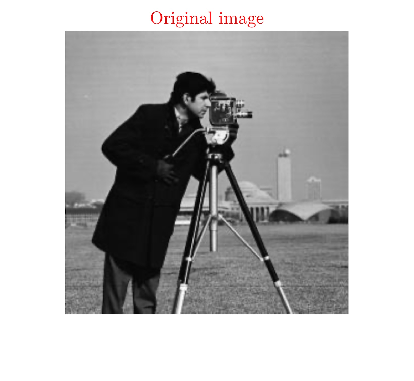
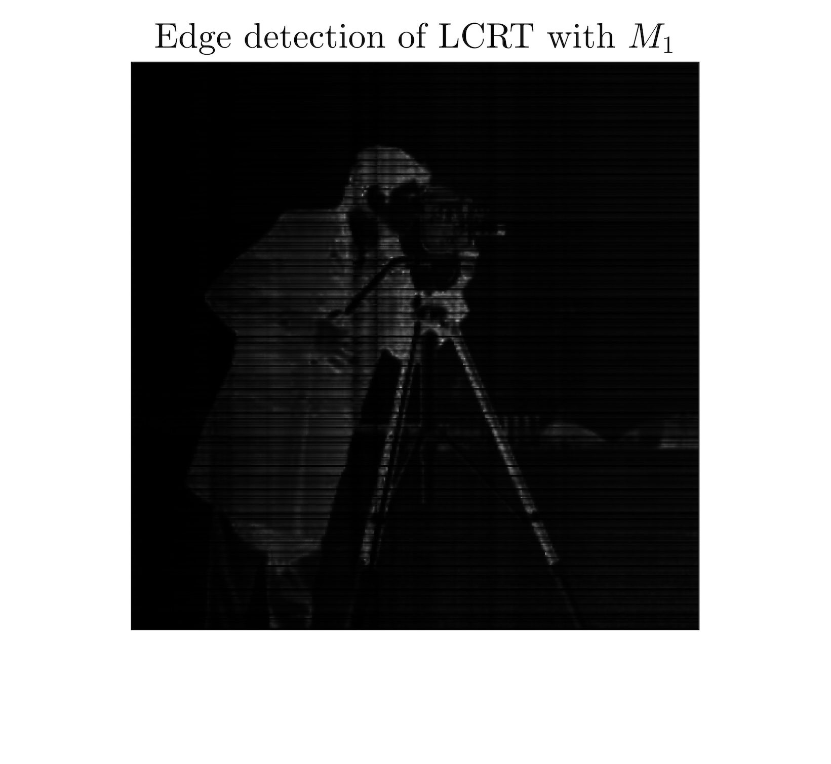
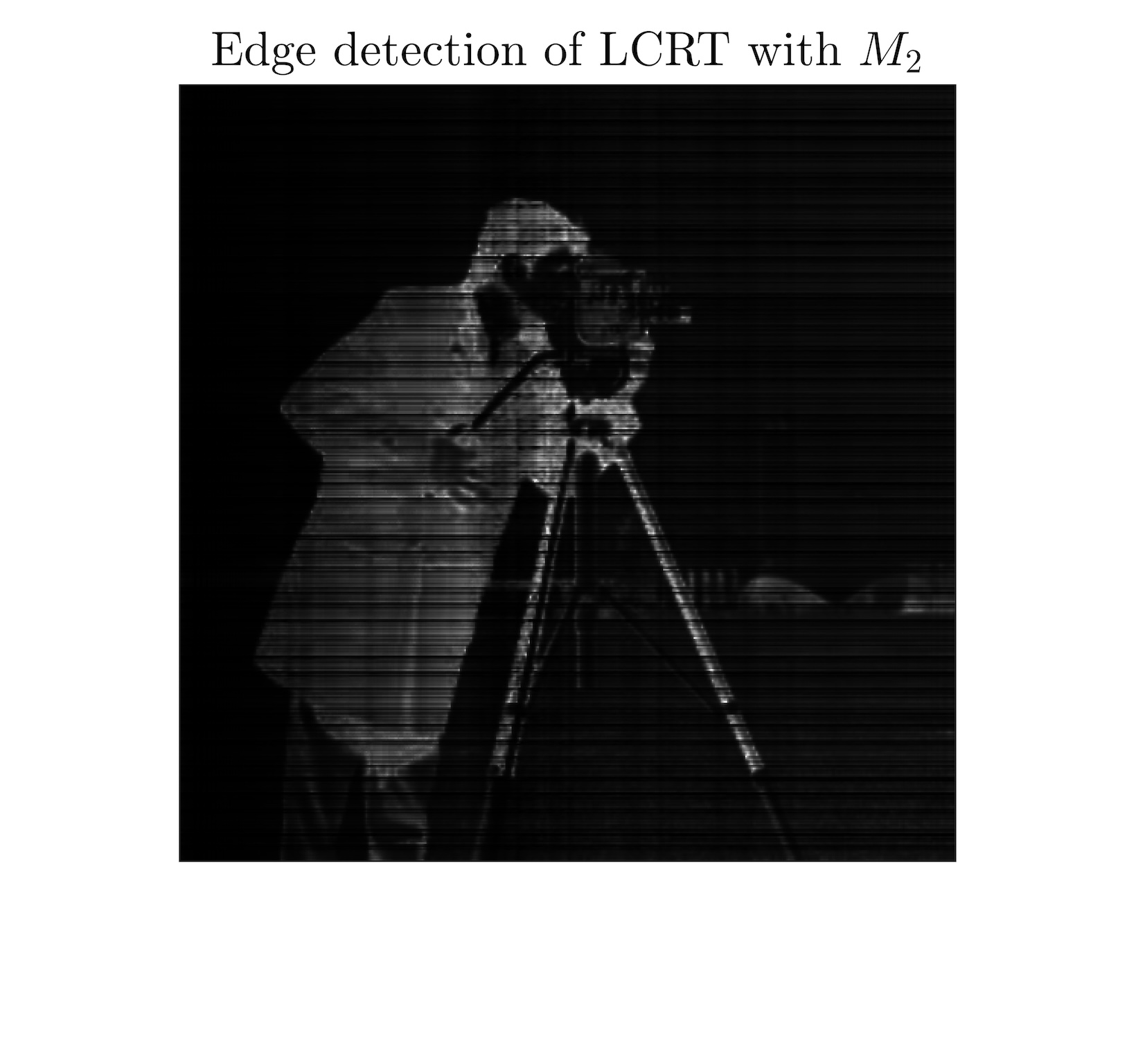
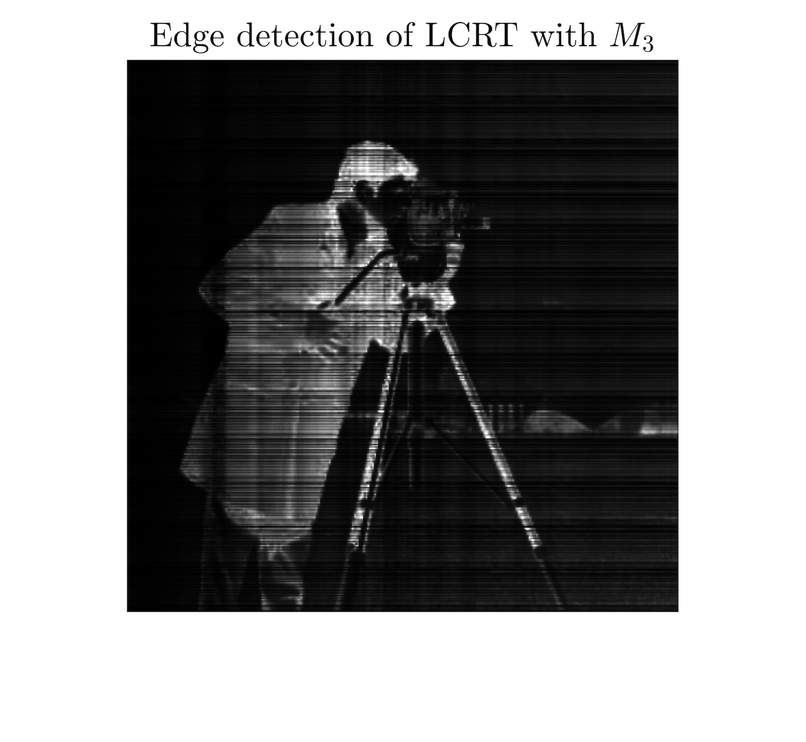
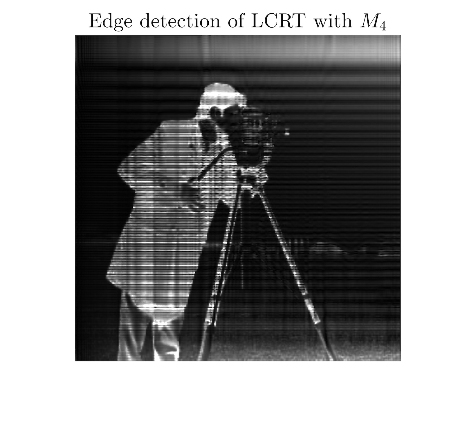
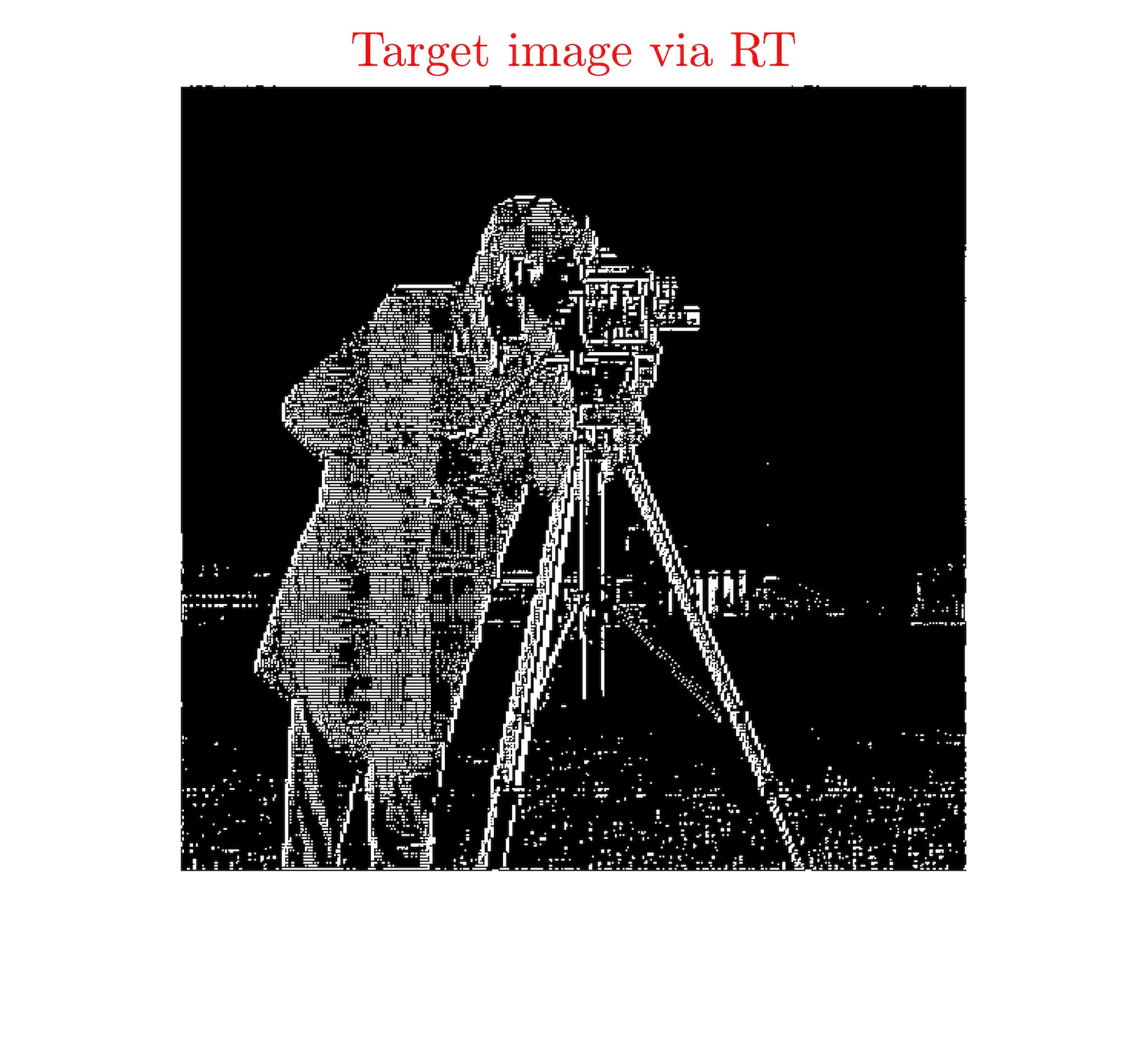
Figure 8: Edge detection using LCRT-IED method on grayscale image Cameraman.

Graph	(b)	(c)	(d)	(e)	(f)
$R_{\mathrm{sc}}^{\mathrm{E}}(A_{2})$	-1000000	-250000	-62500	-625	-1
MSE	0.2625	0.2568	0.2562	0.22	0.1642

Table 1: $R_{\mathrm{sc}}^{\mathrm{E}}$ and MSE corresponding to the edge detection images in Figure 8.

Table 1 presents $R_{\mathrm{sc}}^{\mathrm{E}}$ corresponding to the edge detection images in Figure 8 and the mean squared error (for short, MSE) between the original image and the edge detection images in Figure 8, where $R_{\mathrm{sc}}^{\mathrm{E}}$ is the same as in Definition 4.1 and the MSE is the mean squared error of pixel values between two images which is used to measure the similarity between them. A smaller MSE indicates greater similarity between the two images. As shown in Table 1, when $R_{\mathrm{sc}}^{\mathrm{E}}$ approaches $-1$, the smaller MSE values between the original image and the edge detection images in Figure 8 imply higher similarity between the two images, indicating that the edge strength and continuity of the edge image are good.

We now investigate the effectiveness of the aforementioned introduced LCRT-IED method for local feature extraction in images. In Graph (a) of Figure 9, we divide an image into 9 equally-sized sub-regions. This segmentation aims to assess the local similarity between the edge detection images and the original image by comparing their MSEs within each sub-region. Graphs (b) and (c) in Figure 9 display, respectively, the MSEs between Graphs (a) and (e) and between Graphs (a) and (f) of the aforementioned 9 sub-regions in Figure 8.

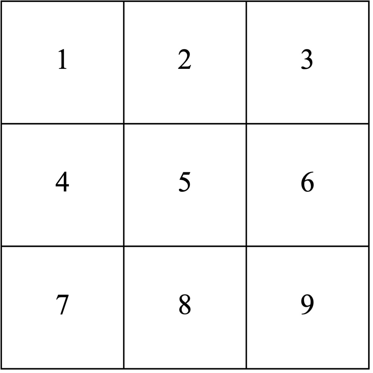
(a) Image Segmentation

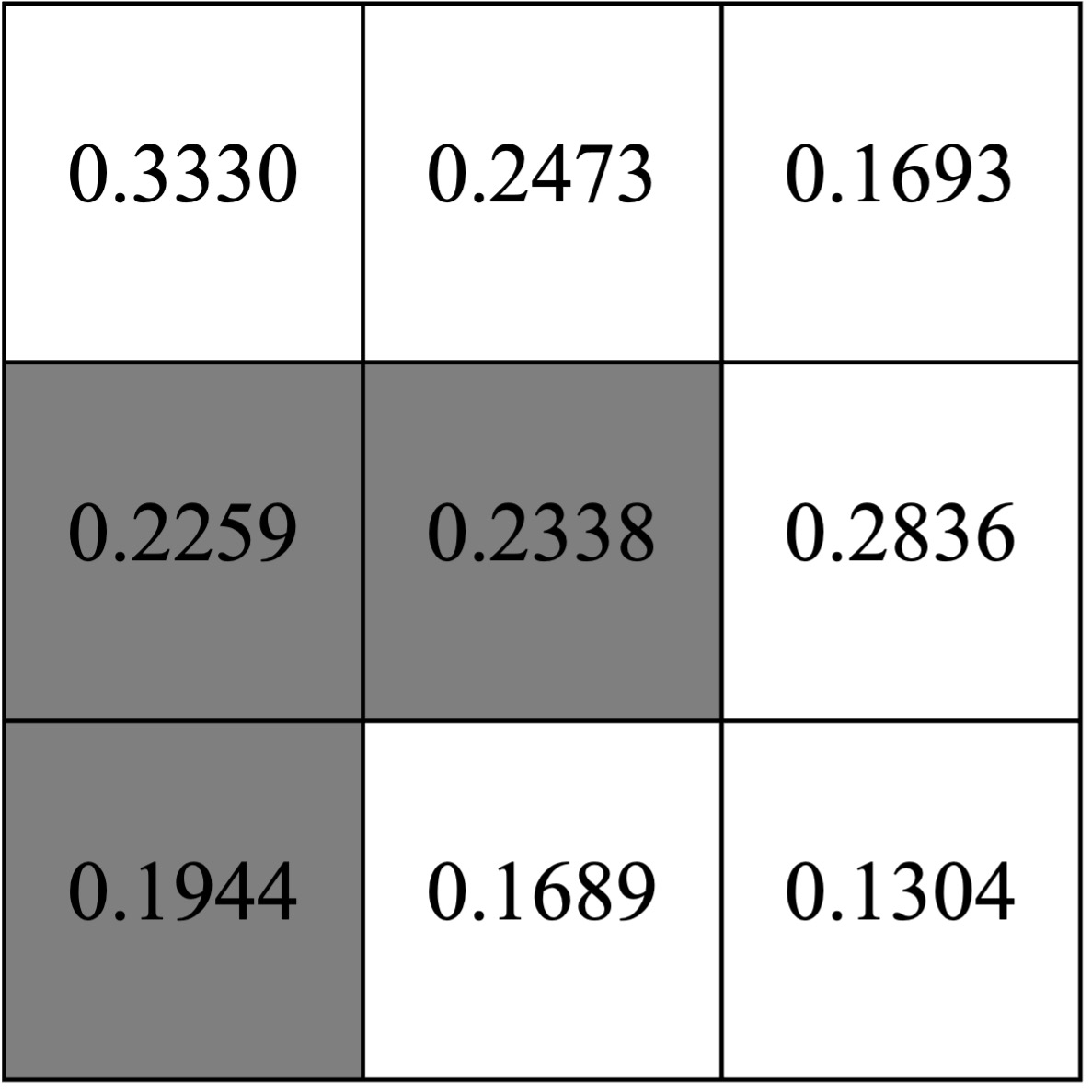
(b) MSE of each sub-region between the Graphs (a) and (e) in Figure 8.

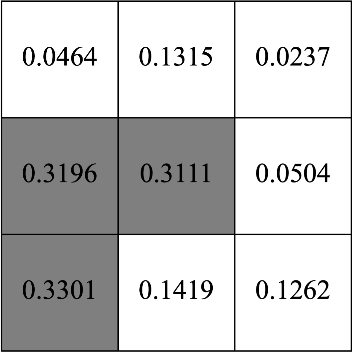
(c) MSE of each sub-region between the Graphs (a) and (f) in Figure 8.

Figure 9: MSE between the original image and the edge detection images in Figure 8 after image segmentation.

The analysis of Table 1 reveals that the MSE between Graphs (a) and (f) in Figure 8 is significantly lower than the one between Graphs (a) and (e) in Figure 8. This suggests that, when the LCRT reduces to the classical Riesz transform, it achieves refined global information extraction. Moreover, comparing Graphs (b) with (c) in Figure 9, we find an interesting phenomenon: for some sub-regions of the aforementioned 9 sub-regions, their MSEs between Graphs (a) and (f) in Figure 8 surpasses those corresponding ones between Graphs (a) and (e) in Figure 8. This interesting phenomenon confirms that the LCRT-IED method possesses dual capabilities: while maintaining stable global edge detection through parameter matrix refinement, it simultaneously excels in local feature extraction, particularly in preserving fine-scale image details for some sub-regions. This is a consequence of the convergence in Theorem 4.2(ii), which is pointwise rather than uniform [see Remark 4.3(i)]. To be precise, while the overall edge effect gradually approaches the best edge effect of the target image from below, in some sub-regions the local edge effect outperforms the corresponding one of the target image.

To ensure both the reliability of the LCRT-IED method introduced above and the generalizability of the conclusions, we now repeat the aforementioned experimental procedure on the other grayscale image.

In Figure 10, Graph (a) is the original test image for edge detection; Graphs (b), (c), (d), (e), and (f) correspond to the edge detection images via the LCRT-IED method by using, respectively, parameter matrices $T_{1}:=(t_{1},t_{2})$ with $t_{1}:=\begin{bmatrix}{0}\ &{1}\\ {-1}\ &{0}\end{bmatrix}$ and $t_{2}:=\begin{bmatrix}{100}\ &{45}\\ {22.2}\ &{100}\end{bmatrix}$, $T_{2}:=(t_{1},t_{3})$ with $t_{3}:=\begin{bmatrix}{100}\ &{70}\\ {\frac{9999}{70}}\ &{100}\end{bmatrix}$, $T_{3}:=(t_{1},t_{4})$ with $t_{4}:=\begin{bmatrix}{100}\ &{300}\\ {33.33}\ &{100}\end{bmatrix}$, $T_{4}:=(t_{1},t_{5})$ with $t_{5}:=\begin{bmatrix}{100}\ &{730}\\ {14.28}\ &{100}\end{bmatrix}$, and $T_{5}:=(t_{1},t_{1})$. In particular, when the parameter matrix is $T_{5}$, in this case the LCRT reduces to the classical Riesz transform. Graphs (b), (c), (d), and (e) demonstrate the gradual enhancement of the edge strength and continuity in the edge images through using different parameter matrices in the LCRT, which gradually approach our target image Graph (f) from below.

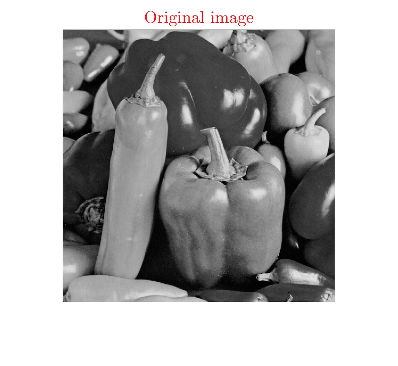
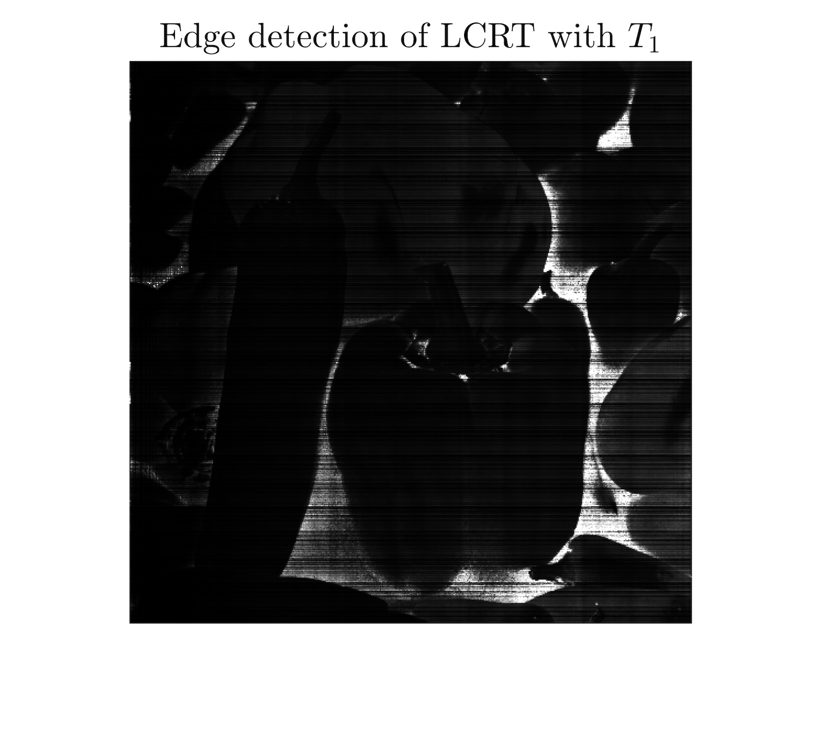
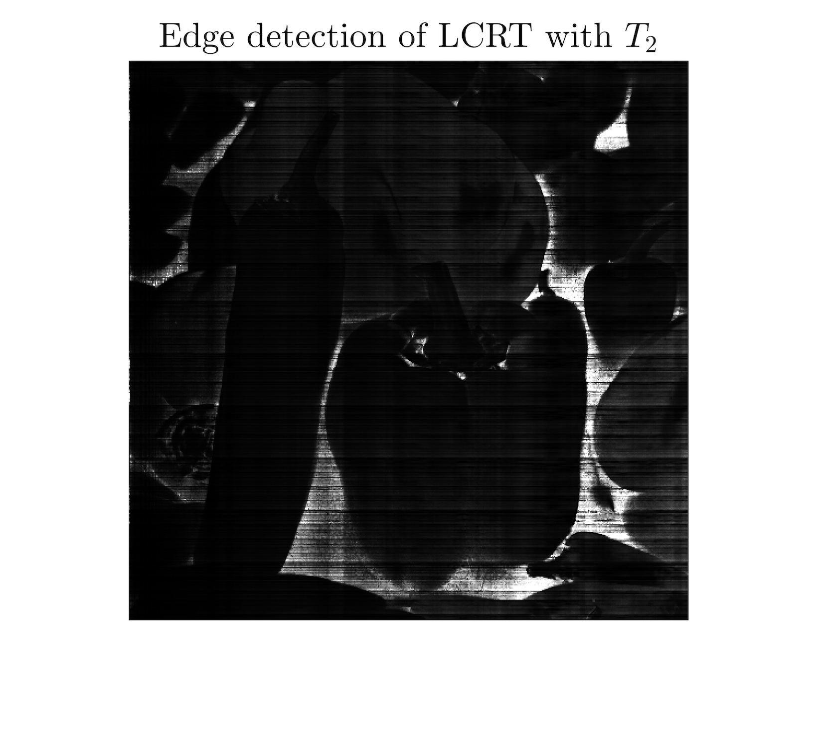
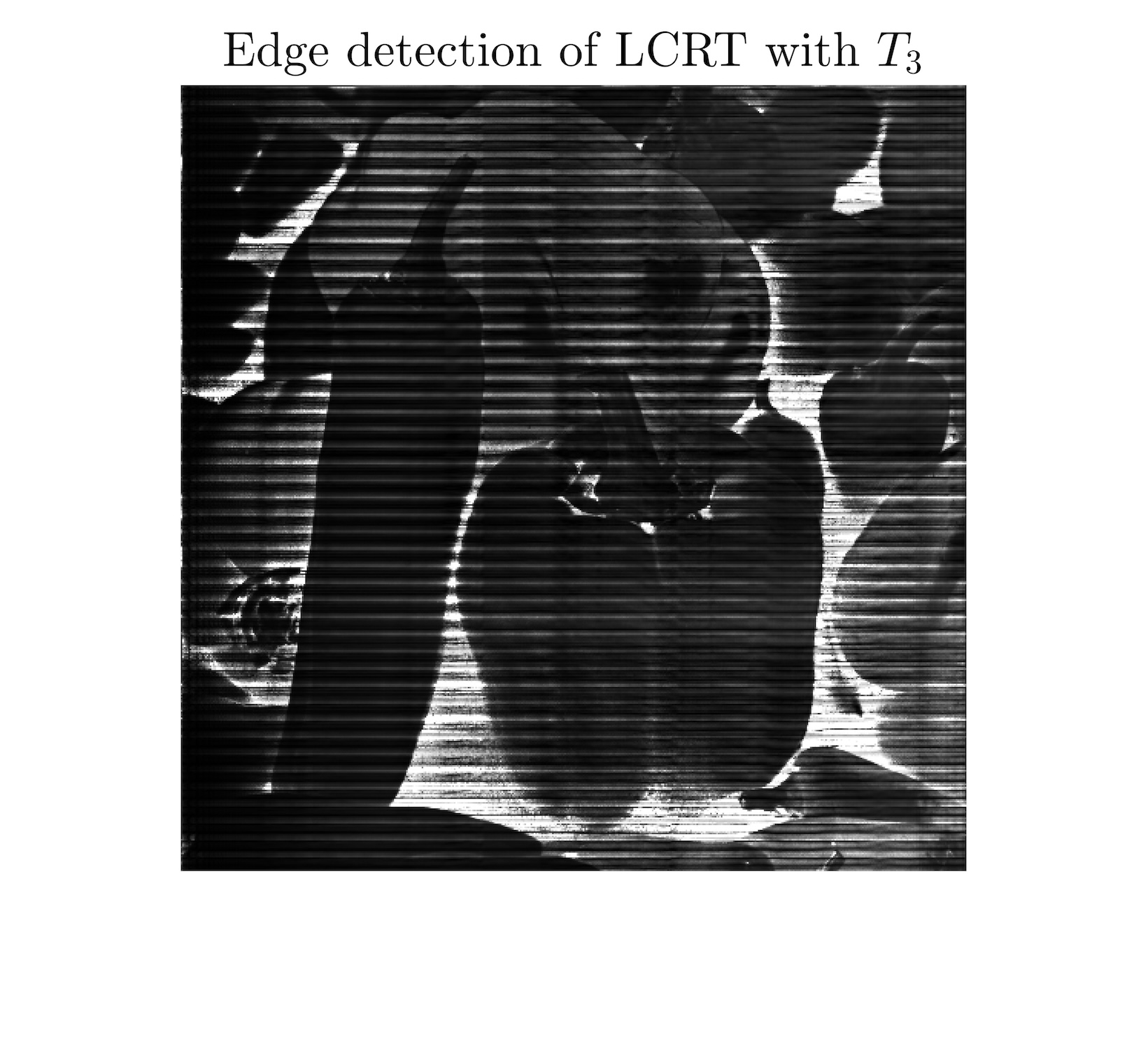
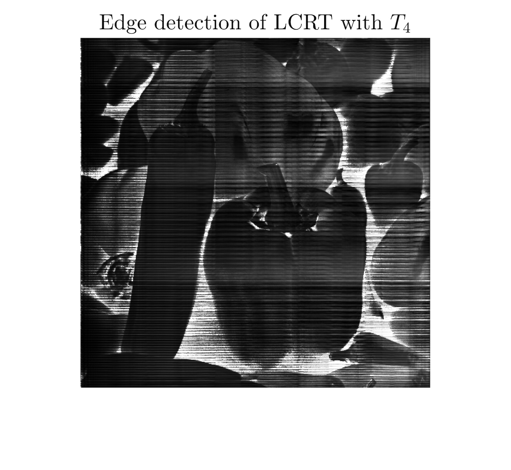
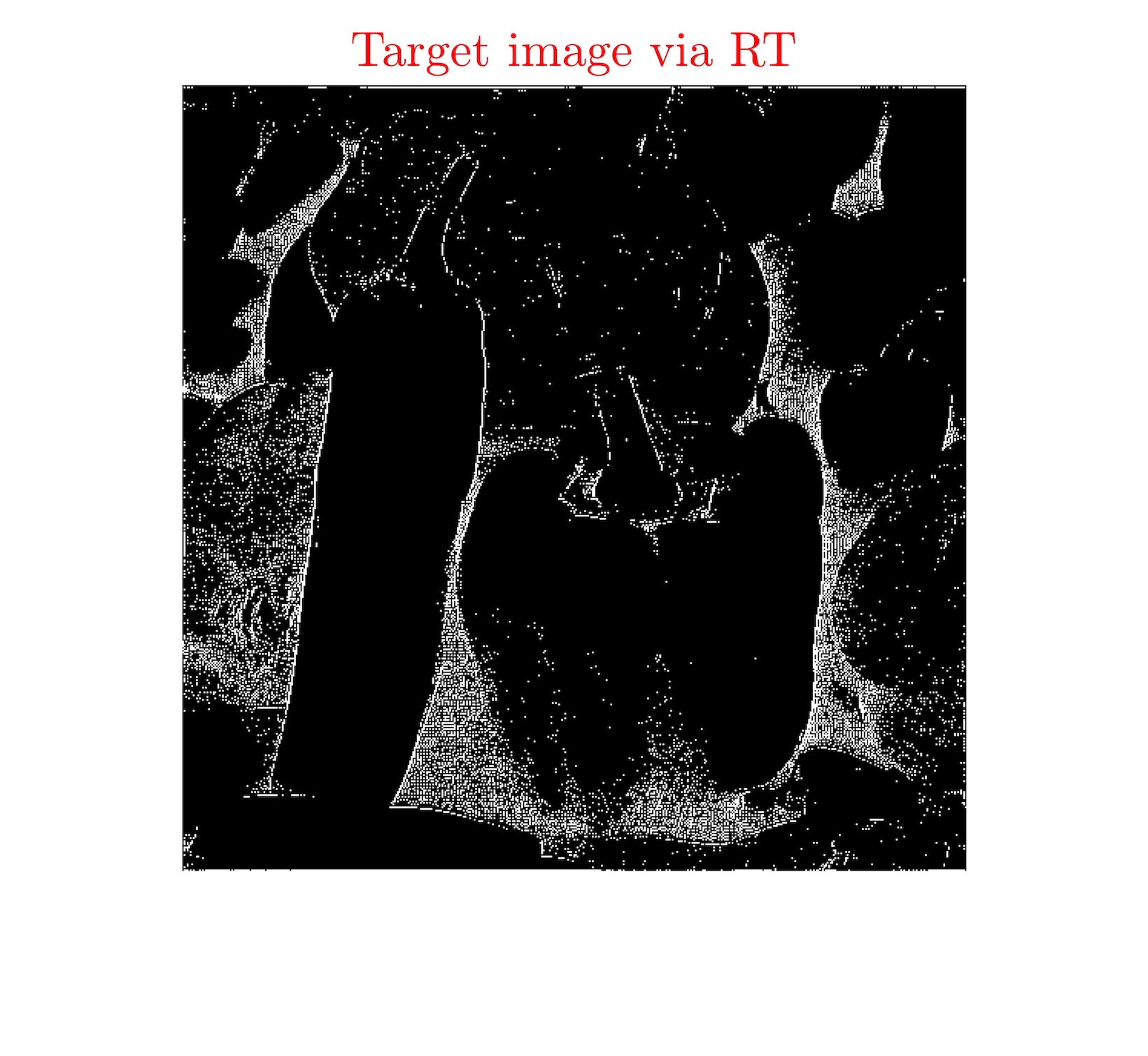
Figure 10: Edge detection using LCRT-IED method on grayscale image Peppers.

Graph	(b)	(c)	(d)	(e)	(f)
$R_{\mathrm{sc}}^{\mathrm{E}}(A_{2})$	51.1024	9.0010	0.4901	0.2025	-1
MSE	0.2197	0.2163	0.2143	0.2009	0.1739

Table 2: $R_{\mathrm{sc}}^{\mathrm{E}}$ and MSE corresponding to the edge detection images in Figure 10.

Table 2 presents $R_{\mathrm{sc}}^{\mathrm{E}}$ corresponding to the edge detection images in Figure 10 and the MSE between the original image and the edge detection images in Figure 10. As shown in Table 2, as $R_{\mathrm{sc}}^{\mathrm{E}}$ approaches $-1$, the MSE between the original image and the edge detection images in Figure 10 becomes increasingly smaller.

Again, we next investigate the effectiveness of the aforementioned introduced LCRT-IED method for local feature extraction in images. Graph (a) of Figure 11 demonstrates dividing an image into 9 equally-sized sub-regions. Graphs (b) and (c) in Figure 11 display, respectively, the MSEs, corresponding to the 9 sub-regions of Graph (a) of Figure 11, between Graphs (a) and (e) of Figure 10 and between Graphs (a) and (f) of Figure 10.

As demonstrated by the experimental results from Figures 10 and 11 and Table 2, the findings of this study align consistently with the results presented in Figures 8 and 9 and Table 1, thereby confirming that the LCRT-IED method exhibits reliability and generalizability.

In Figures 8 and 10, we perform LCRT-IED method on two different grayscale images using different parameter matrices. Indeed, our LCRT-IED method can also be directly applied to RGB images, achieving similar experimental results. However, the processing approach slightly differs when handling RGB images. To be precise, we first divide the RGB image into the red, the green, and the blue channels. Each color channel is treated as a grayscale image, and we then apply the LCRT-IED method with the same parameter matrices to each channel. Finally, we recombine these three channels to form the RGB image.

(a) Image segmentation.

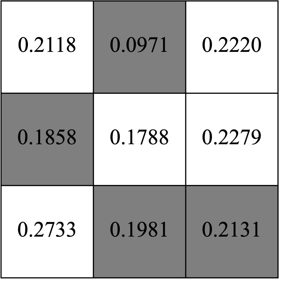
(b) MSE of each sub-region between the Graphs (a) and (e) in Figure 10.

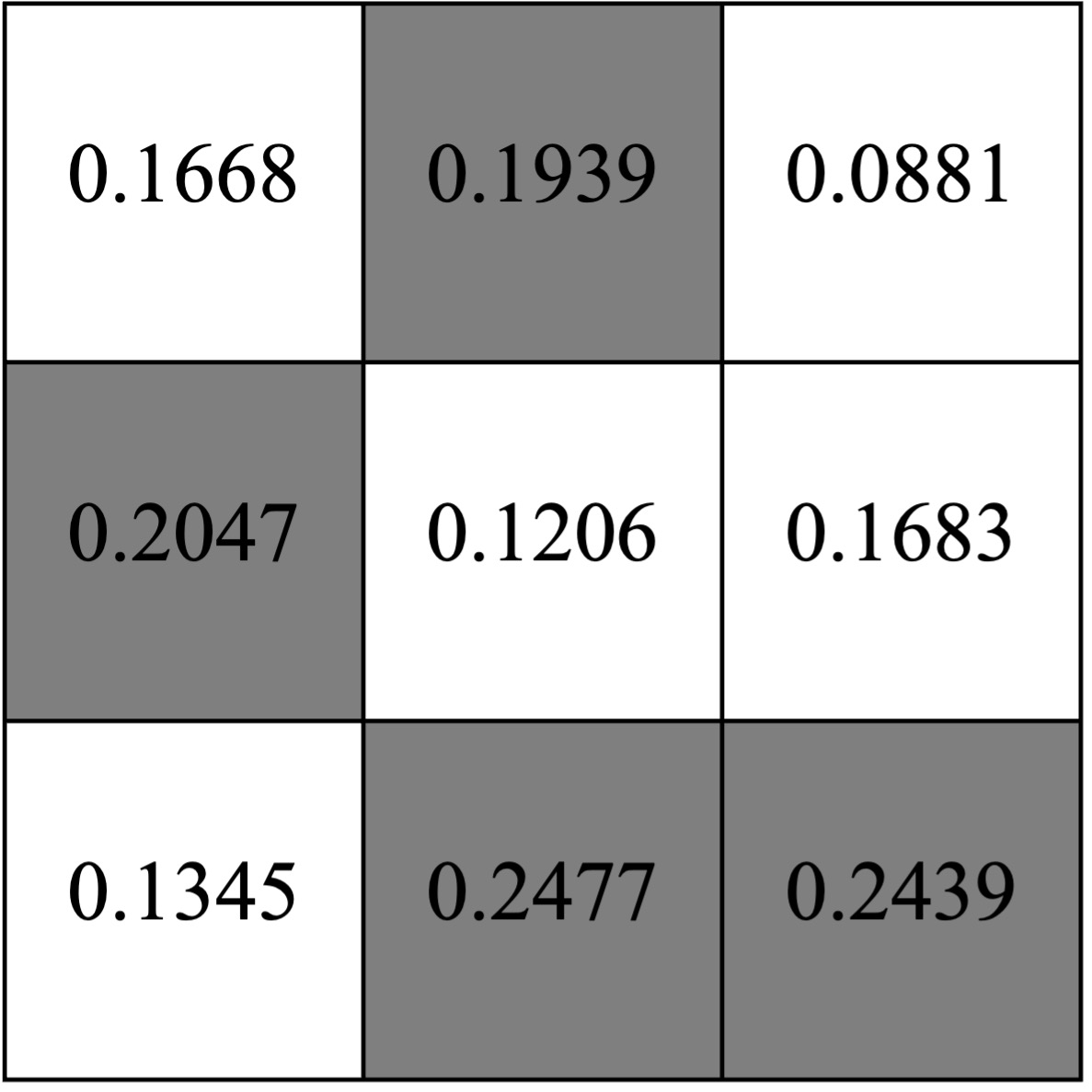
(c) MSE of each sub-region between the Graphs (a) and (f) in Figure 10.

Figure 11: MSE between the original image and the edge detection images in Figure 10 after image segmentation.

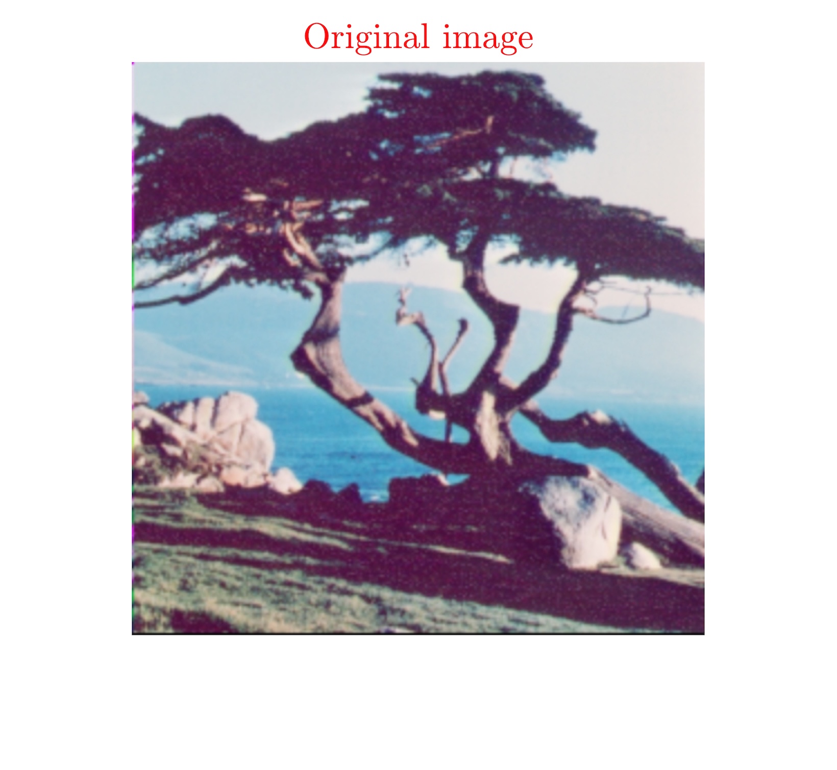
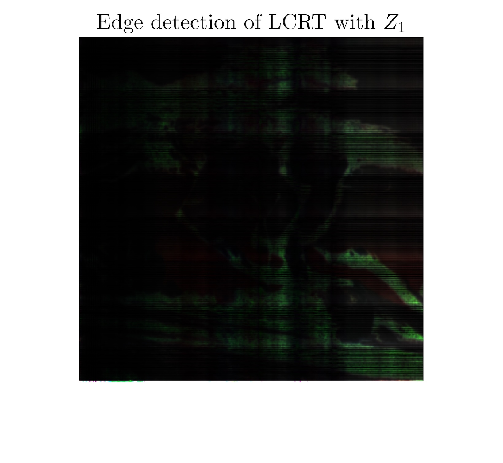
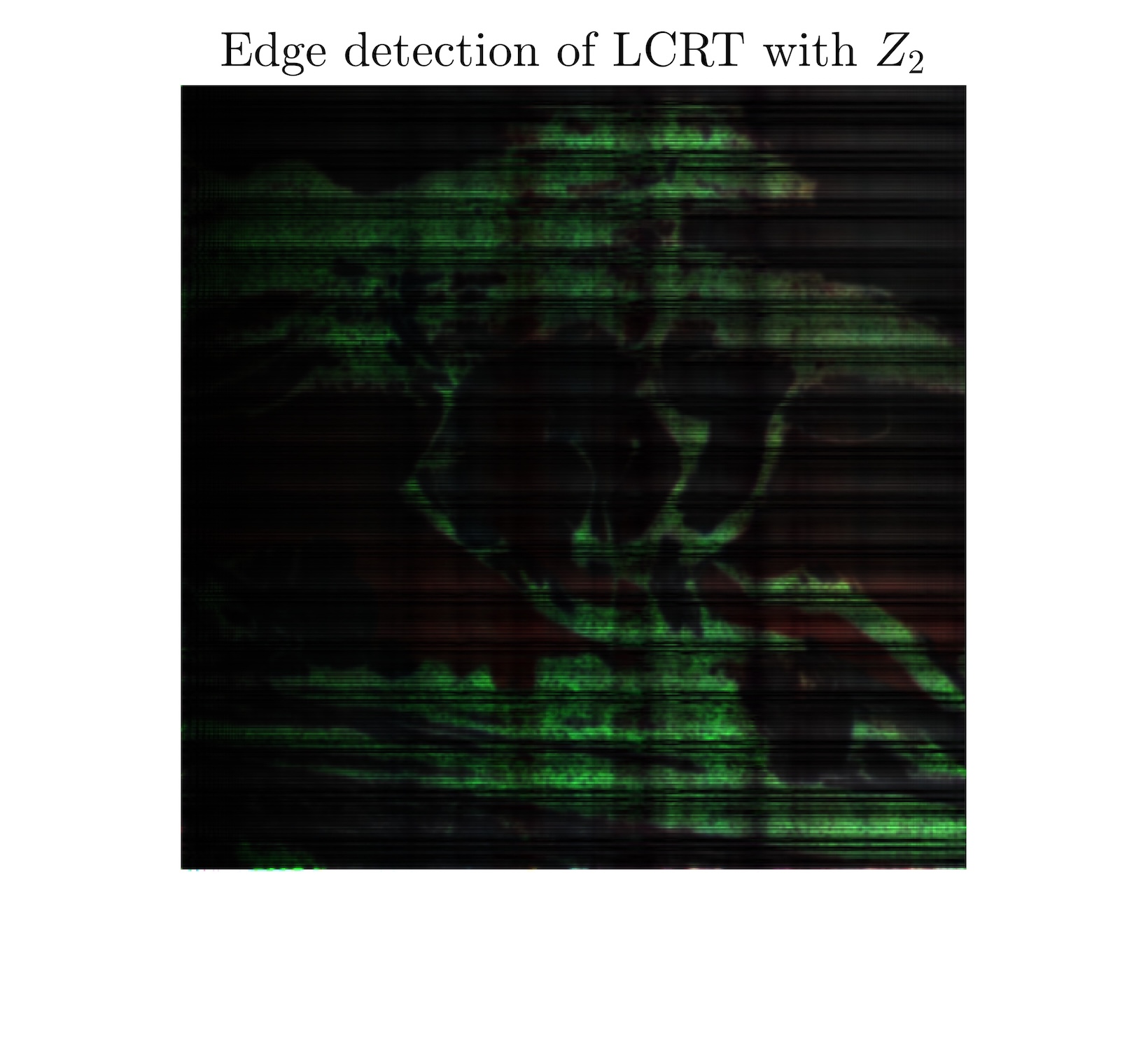
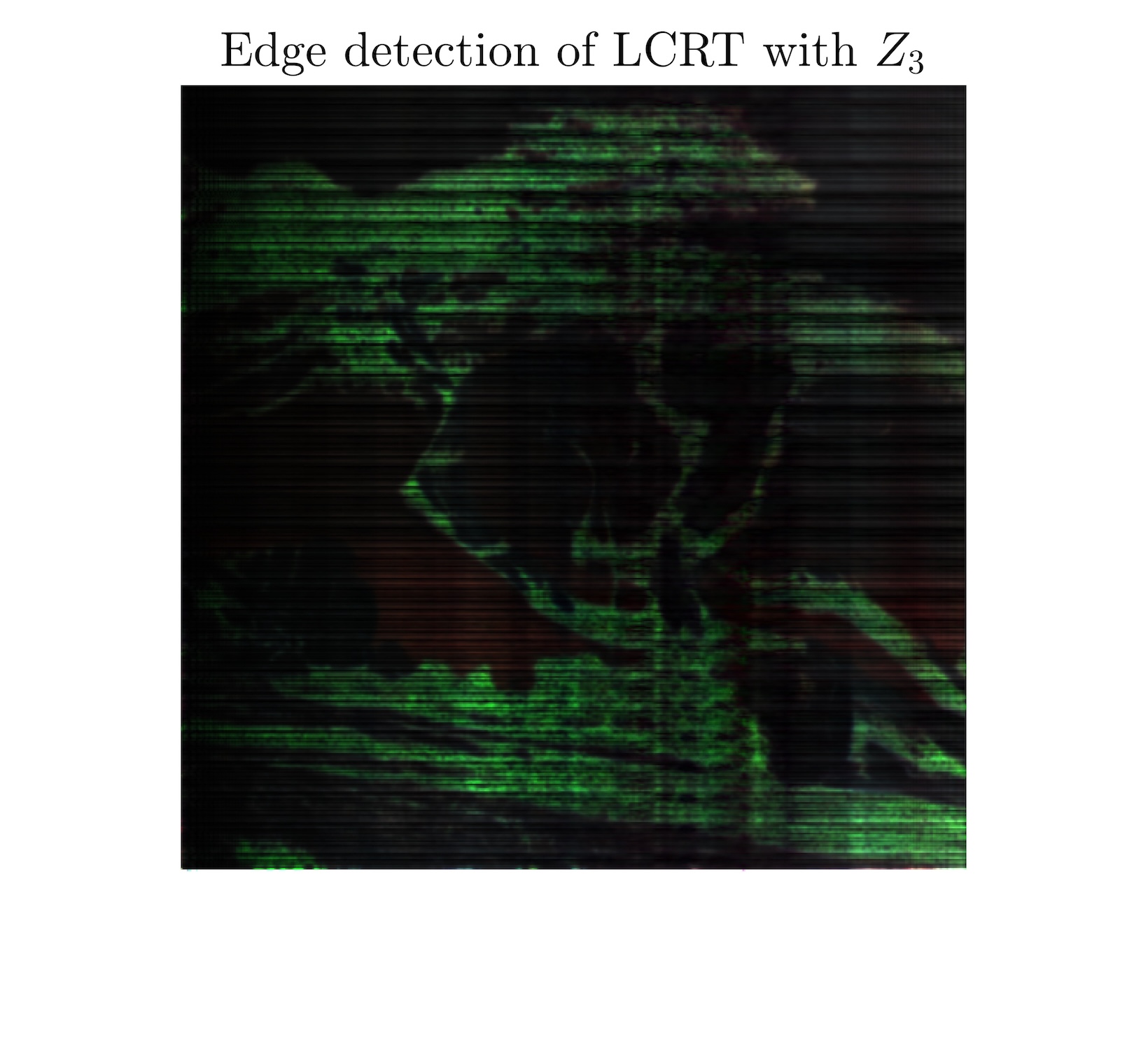
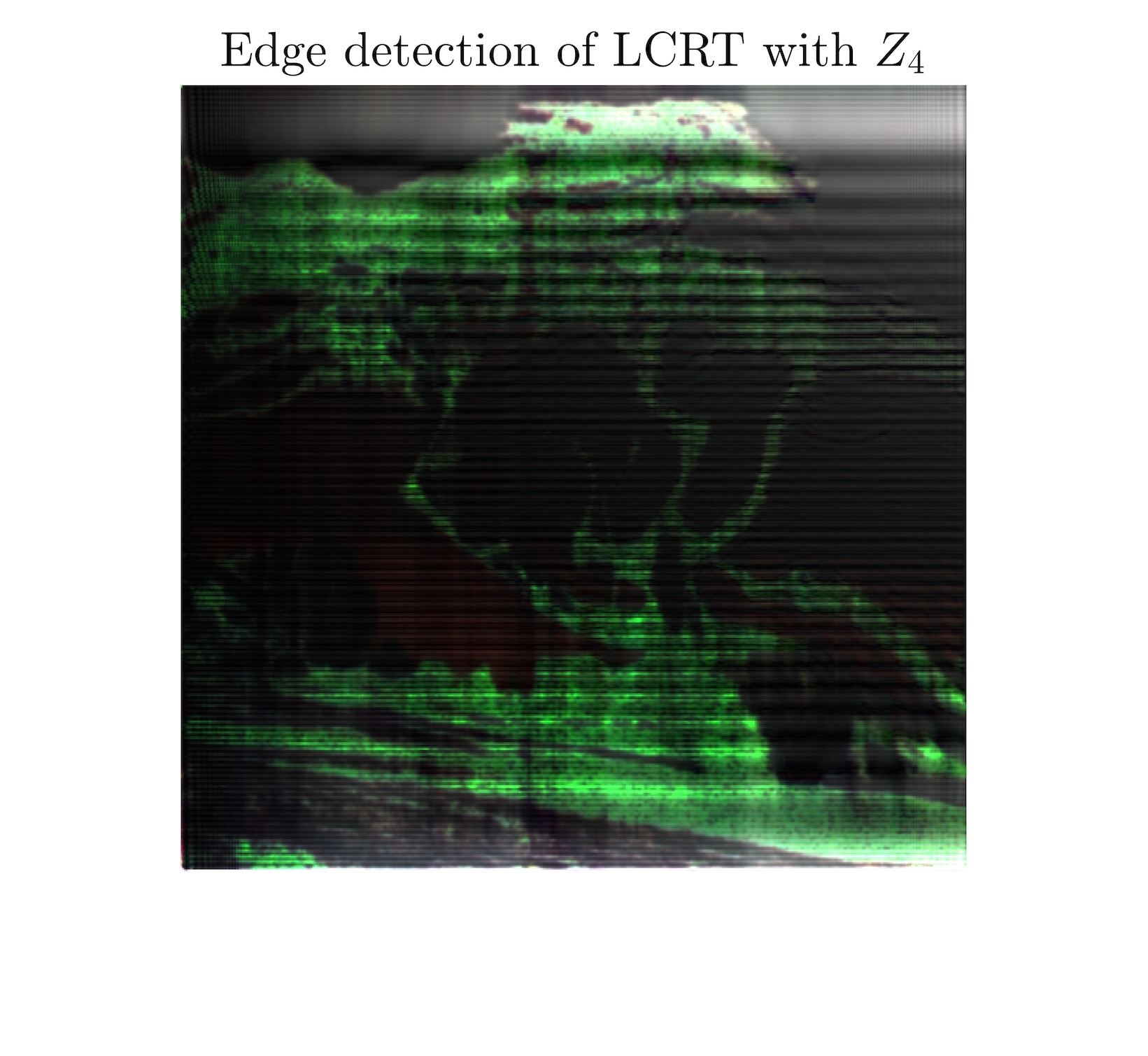
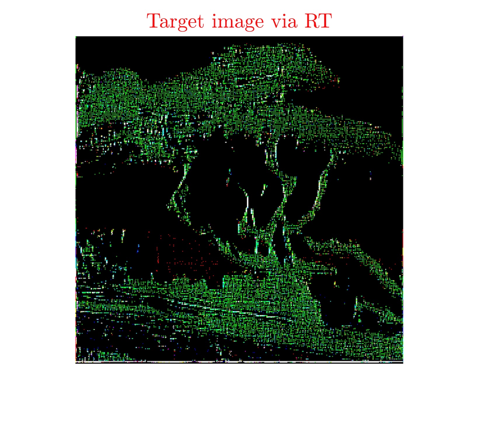
Figure 12: Edge detection using LCRT-IED method on RGB image.

In Figure 12, we use the classic RGB image in Graph (a) as the original test image; Graphs (b), (c), (d), (e), and (f) correspond to the edge detection images via the LCRT-IED method by using, respectively, parameter matrices $Z_{1}:=(z_{1},z_{2})$ with $z_{1}:=\begin{bmatrix}{0}\ &{1}\\ {-1}\ &{0}\end{bmatrix}$ and $z_{2}:=\begin{bmatrix}{0}\ &{400}\\ {-\frac{1}{400}}\ &{0}\end{bmatrix}$, $Z_{2}:=(z_{1},z_{3})$ with $z_{3}:=\begin{bmatrix}{0}\ &{200}\\ {-0.005}\ &{0}\end{bmatrix}$, $Z_{3}:=(z_{1},z_{4})$ with $z_{4}:=\begin{bmatrix}{0}\ &{125}\\ {-0.008}\ &{0}\end{bmatrix}$, $Z_{4}:=(z_{1},z_{5})$ with $z_{5}:=\begin{bmatrix}{0}\ &{22}\\ {-\frac{1}{22}}\ &{0}\end{bmatrix}$, and $Z_{5}:=(z_{1},z_{1})$. In particular, when the parameter matrix is $Z_{5}$, in this case the LCRT reduces to the classical Riesz transform. Graphs (b), (c), (d), and (e) demonstrate the gradual enhancement of the edge strength and continuity in the edge images through using different parameter matrices in the LCRT, which gradually approach our target image Graph (f).

Graph	(b)	(c)	(d)	(e)	(f)
$R_{\mathrm{sc}}^{\mathrm{E}}(A_{2})$	-160000	-40000	-15625	-484	-1
MSE(red)	0.2933	0.2731	0.2659	0.2148	0.1193
MSE(green)	0.3095	0.2975	0.2914	0.2688	0.1729
MSE(blue)	0.3528	0.3319	0.3215	0.2697	0.1642

Table 3: $R_{\mathrm{sc}}^{\mathrm{E}}$ and MSE corresponding to the edge detection images in Figure 12.

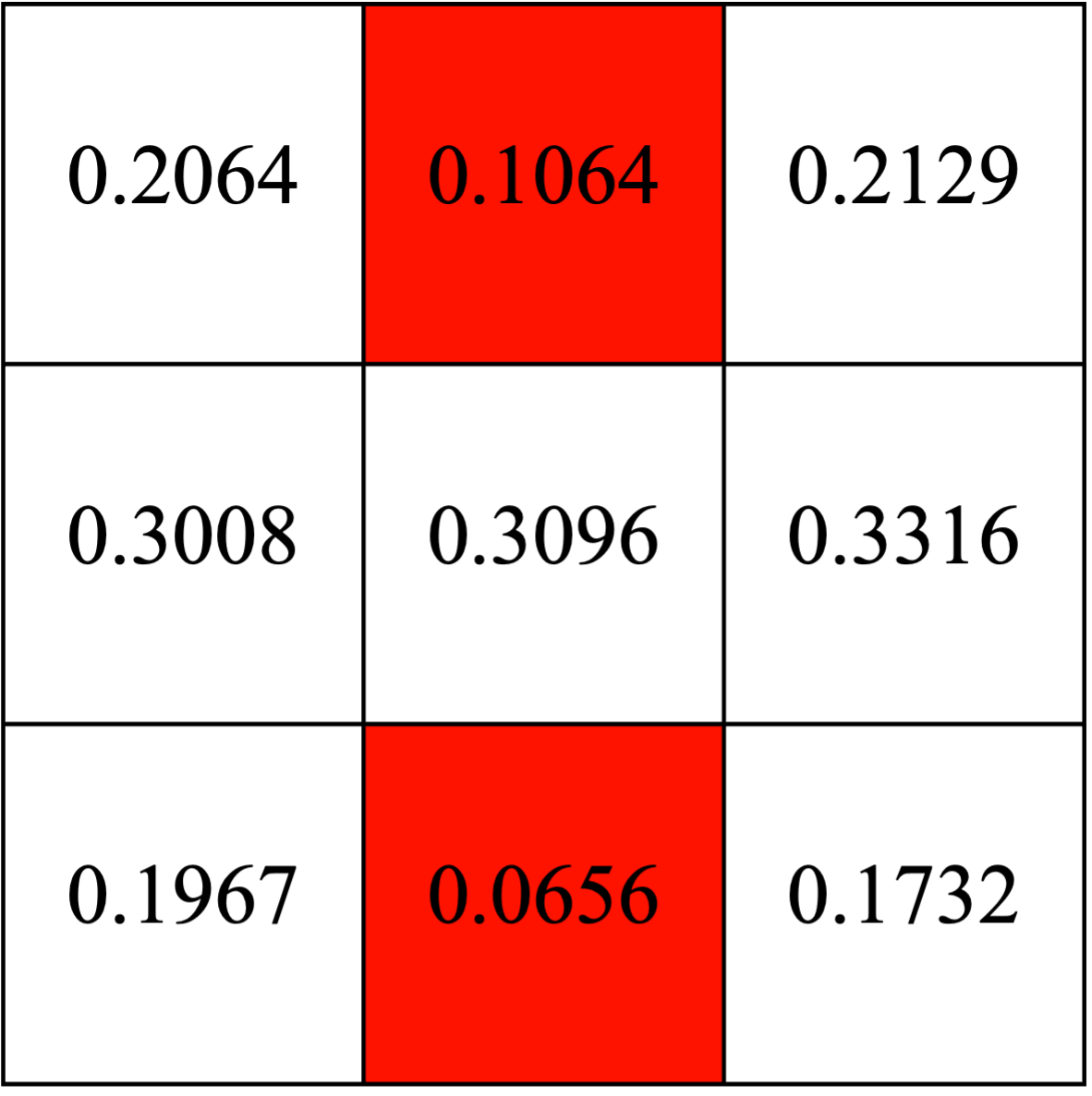
(a) MSE of the Red Channel between (a) and (e) in Figure 12.

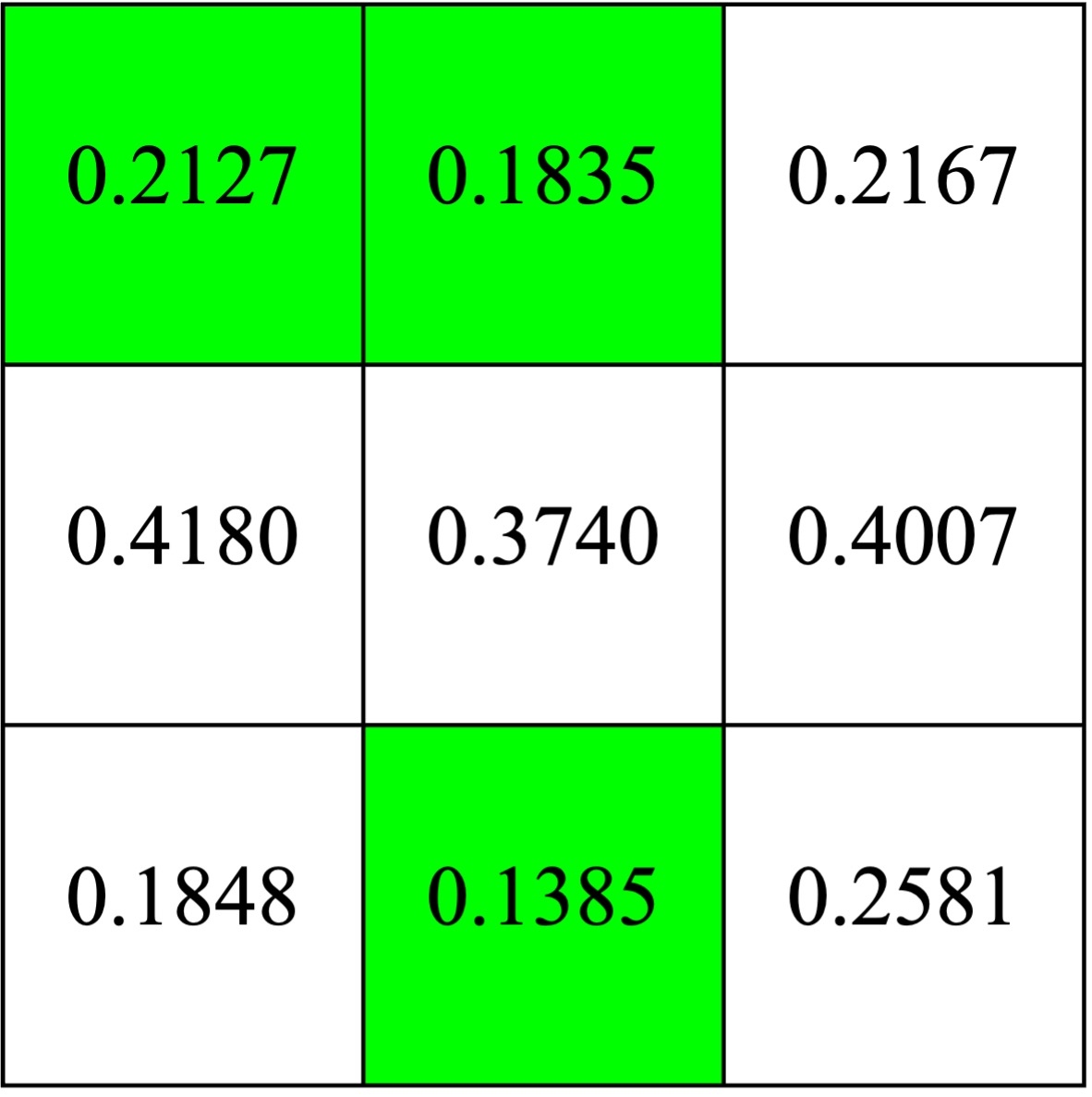
(b) MSE of the green channel between (a) and (e) in Figure 12.

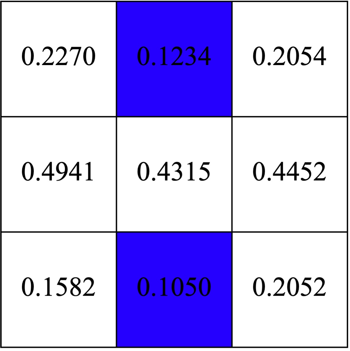
(c) MSE of the blue channel between (a) and (e) in Figure 12.

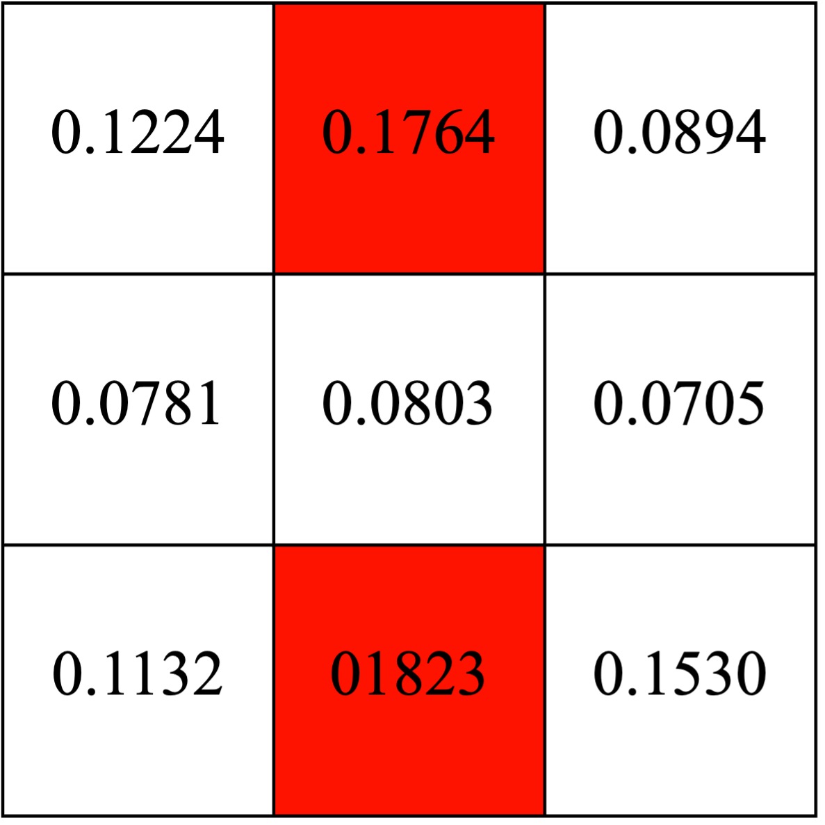
(d) MSE of the red channel between (a) and (f) in Figure 12.

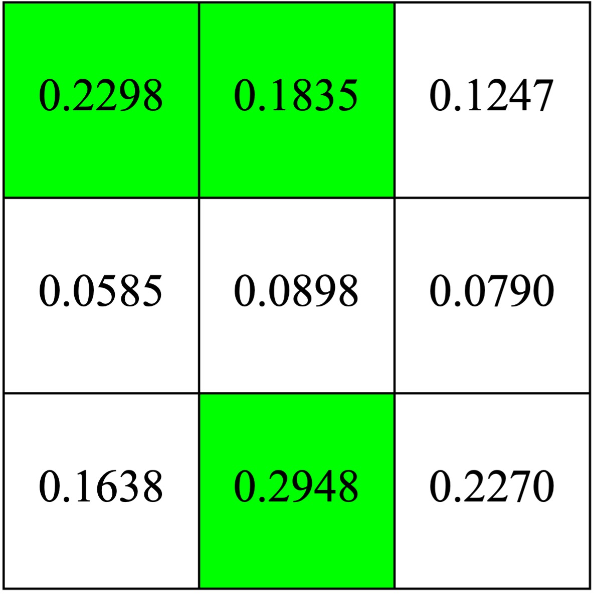
(e) MSE of the green channel between (a) and (f) in Figure 12.

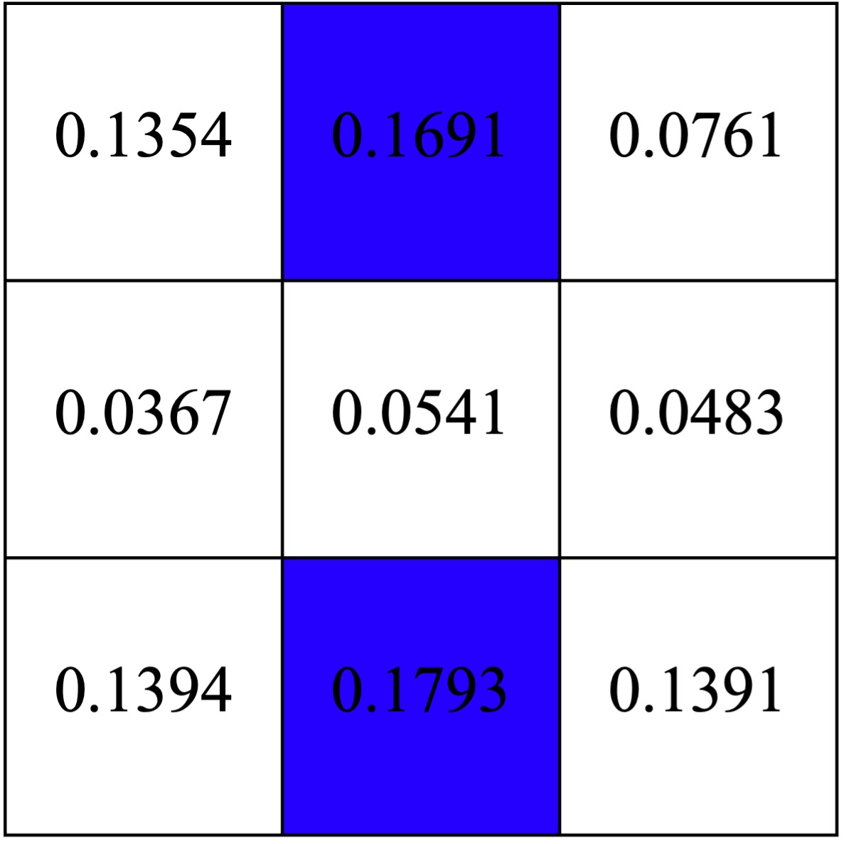
(f) MSE of the blue channel between (a) and (f) in Figure 12.

Figure 13: MSE between the original image and the edge detection images in Figure 12 in the red, the green, and the blue channels after image segmentation.

Since the original test image in Figure 12 is an RGB image, Table 3 presents the $R_{\mathrm{sc}}^{\mathrm{E}}$ corresponding to the edge detection images in Figure 12, as well as the MSE between the original image and the edge detection images in Figure 12, respectively, on the red, the green, and the blue channels. As shown in Table 3, when $R_{\mathrm{sc}}^{\mathrm{E}}$ approaches $-1$, the MSE between the original image and the edge detection images in Figure 12 on all three channels increasingly decreases, indicating the higher degree of similarity between them.

Figure 13 shows the MSEs, respectrvely, between Graphs (a) in Figure 12 and Graphs (e) and (f) in Figure 12 about each sub-region in the red, the green, and the blue channels after the same image segmentation as in Figure 9. Particularly, Graphs (a), (b), and (c) in Figure 13 display the MSEs, respectively, between Graphs (a) and (f) in Figure 12 the aforementioned 9 sub-regions in the red, the green, and the blue channels. Graphs (d), (e), and (r) in Figure 13 display the MSEs, respectively, between images (a) and (e) in Figure 12 about the aforementioned 9 sub-regions in the red, the green, and the blue channels.

As demonstrated by the experimental data in Figures 12 and 13, as well as Table 3, the results for RGB images and the two types of grayscale images show the high degree of consistency. This validates that the LCRT-IED method also possesses excellent feature extraction capabilities in RGB image processing.

Based on the results of the three sets of experiments mentioned above, we find that this new LCRT-IED method introduced above has two key advantages:

1. Effective control of edge properties: The LCRT-IED method is able to gradually control the image edge strength and continuity.

2. Local feature extraction: The LCRT-IED method demonstrates the significant capability in feature extraction about some local regions, enabling more precise preservation of image detail information.

These advantages highlight the practical value of the LCRT-IED method for image processing tasks in complex scenarios. When we reduce from LCRTs to fractional Riesz transforms, selecting a specific fractional order can effectively extract local information in specific directions of the image. It is worth mentioning that the experimental results presented in this article do not require final binarization like the fractional Riesz transform edge detection method in [19] and, moreover, the results are equally striking. This can be attributed to the fact that the LCT is able to perform not only rotations but also scaling operations in the time-frequency plane. Furthermore, the LCRT-IED method also performs exceptionally well when processing RGB images.

Remark 4.4.

By observing the results of the three sets of experiments above, we notice that, in the above experiments, we always fix the parameter matrix $A_{1}$ in LCRTs $\{R_{1}^{\boldsymbol{A}},R_{2}^{\boldsymbol{A}}\}$ with $\boldsymbol{A}:=(A_{1},A_{2})$ as in Definition 2.5 with $n=2$ and only allow $A_{2}$ to vary. This naturally raises a question: if we instead fix $A_{2}$ and let $A_{1}$ vary, would the same effect be observed? However, experimental validation shows that this is not the case, and only some weak edge information is available in this case. The deep reason for this lies in the fact that the roles of $R_{1}^{\boldsymbol{A}}$ and $R_{2}^{\boldsymbol{A}}$ are not symmetric in the local direction $\theta(\boldsymbol{x})$ in (4.1), leading to an essential difference in their effectiveness within the model under consideration.

4.2 Advantages and Features

In image processing, finely tuning the strength and the continuity of image edges can significantly enhance processing effects. The advantages and features of LCRT-IED methods can be summarized as follows:

1. Improvement of the efficiency of image matching: In image matching, we are confronted with a challenging task: how to efficiently identify images that match the target image from a vast database containing millions of images. To address this challenge, we can employ a multi-stage processing method based on edge strength and continuity. This method adopts a hierarchical strategy to refine the matching process step by step. Initially, the LCRT-IED method is applied to extract edge features with varying strengths and continuities. Subsequently, these features are used to train and evaluate models, thereby selecting the refined edge-detected images for subsequent matching stages. By combining coarse matching and fine matching, dissimilar images are filtered out, and the focus is narrowed down to candidate images with high similarity. Finally, the best-matching image is determined through pairwise comparison. This multi-stage approach not only simplifies the complexity of the matching process but also demonstrates significant advantages when dealing with large-scale image databases.

2. Refinement of feature extraction: Edges, as important indicators of image brightness changes, are often closely related to the contours or the boundaries of objects under consideration. Edge detection techniques can effectively capture this critical information, laying a solid foundation for deeper image analysis and interpretation. For example, in medical image analysis, edge detection help to identify the boundaries of tumors, and, in facial recognition systems, edge detection can extract facial features. By adjusting the strength and the continuity of the edges, these features can be more accurately identified and emphasized, thus improving the accuracy of image analysis.

3. Image refinement processing: By employing advanced edge detection techniques, key information in the image can be accurately retained while cleverly removing unnecessary pixel details. For example, in the manufacturing industry, image refinement processing techniques can be used to inspect product surfaces. By accurately preserving edge information, surface defects such as scratches or blemishes can be quickly identified. This fine-tuning not only significantly reduces computational burden and speeds up processing, but also greatly enhances the intuitiveness and the efficiency of image analysis.

4. Catalyst for subsequent processing: Finely tuning the strength and the continuity of image edges provides a solid and precise foundation for subsequent tasks such as image segmentation, object recognition, and tracking. The refined edge information simplifies the accurate identification and the localization of target objects, significantly improving the efficiency and the accuracy of follow-up processing tasks. This ensures the smoothness and the efficiency of the entire image analysis process and provides strong support for subsequent stages of image processing.

5 Conclusions

This article introduces LCRTs on the basis of LCTs and Riesz transforms. We also further perform a series of numerical simulations on images using both LCRTs and HLCHTs. By comparing these simulation experiments, we validate their respective effectiveness and highlight the differences among them. In addition, we apply LCRTs to refine image edge detection and propose a new LCRT image edge detection method, namely the LCRT-IED method, by first introducing the concept of the sharpness $R^{\mathrm{E}}_{\mathrm{sc}}$ of the edge strength and continuity of images associated with the LCRT. This method is able to gradually control the edge strength and continuity by subtly tuning the parameter matrices of LCRTs based on the sharpness $R^{\mathrm{E}}_{\mathrm{sc}}$ and performs well in feature extraction on some local regions. Moreover, this method is not only applicable to grayscale images but also works well with RGB images. This new method can be regarded as the refinement of the fractional Riesz transform edge detection method in [19]. Serving as a catalyst for subsequent image processing, it is of great significance for image matching, image feature extraction, and image refinement processing.

Data availability

No data was used for the research described in the article.

Shuhui Yang and Dachun Yang (Corresponding author)

Laboratory of Mathematics and Complex Systems (Ministry of Education of China), School of Mathematical Sciences, Beijing Normal University, Beijing 100875, The People’s Republic of China

E-mails: shuhuiyang@bnu.edu.cn (S. Yang)

E-mails: dcyang@bnu.edu.cn (D. Yang)

Zunwei Fu

School of Mathematics and Statistics, Linyi University, Linyi 276000, The People’s Republic of China; College of Information Technology, The University of Suwon, Hwaseong-si 18323, South Korea

E-mail: zwfu@suwon.ac.kr

Yan Lin and Zhen Li

School of Science, China University of Mining and Technology, Beijing 100083, The People’s Republic of China

E-mails: linyan@cumtb.edu.cn (Y. Lin)

E-mails: lizhen@student.cumtb.edu.cn (Z. Li)

References

- [1] S. A. Abbas, Q. Sun and H. Foroosh, An exact and fast computation of discrete Fourier transform for polar and spherical grid, IEEE Trans. Signal Process. 65 (2017), 2033–2048.
- [2] V. Bargmann, On a Hilbert space of analytic functions and an associated integral transform, Comm. Pure Appl. Math. 14 (1961), 187–214.
- [3] B. Barshan, M. A. Kutay and H. M. Ozaktas, Optimal filtering with linear canonical transformations, Opt. Commun.135 (1997), 32–36.
- [4] M. J. Bastiaans, The Wigner distribution function applied to optical signals and systems, Opt. Commun. 25 (1978), 26–30.
- [5] L. M. Bernardo, ABCD matrix formalism of fractional Fourier optics, Opt. Eng. 35 (1996), 732–740.
- [6] N. Bi, Q. Sun, D. Huang, Z. Yang and J. Huang, Robust image watermarking based on multiband wavelets and empirical mode decomposition, IEEE Trans. Image Process. 16 (2007), 1956–1966.
- [7] B. Boashash, Estimating and interpreting the instantaneous frequency of a signal. I. Fundamentals, Proc. IEEE 80 (1992), 520–538.
- [8] B. Boashash, Estimating and interpreting the instantaneous frequency of a signal. II. Algorithms and applications, Proc. IEEE 80 (1992), 540–568.
- [9] G. Chaple and R. D. Daruwala, Design of Sobel operator based image edge detection algorithm on FPGA, 2014 International Conference on Communication and Signal Processing, 2014, pp. 788–792, IEEE.
- [10] W. Chen, Z. Fu, L. Grafakos and Y. Wu, Fractional Fourier transforms on and applications, Appl. Comput. Harmon. Anal. 55 (2021), 71–96.
- [11] Y. Chen, C. Cheng and Q. Sun, Graph Fourier transform based on singular value decomposition of the directed Laplacian, Sampl. Theory Signal Process. Data Anal. 21 (2023), Paper No. 24, 28 pp.
- [12] C. Cheng, Y. Chen, Y. J. Lee and Q. Sun, SVD-based graph Fourier transforms on directed product graphs, IEEE Trans. Signal Inform. Process. Netw. 9 (2023), 531–541.
- [13] S. A. Collins, Lens-system diffraction integral written in terms of matrix optics, J. Opt. Soc. Amer. 60 (1970), 1168–1177.
- [14] C. Deng, G. Wang and X. Yang, Image edge detection algorithm based on improved canny operator, 2013 International Conference on Wavelet Analysis and Pattern Recognition, 2013, pp. 168–172, IEEE.
- [15] N. C. Dias, M. de Gosson and J. N. Prata, A metaplectic perspective of uncertainty principles in the linear canonical transform domain, J. Funct. Anal. 287 (2024), Paper No. 110494, 54 pp.
- [16] J. J. Ding and S. C. Pei, 2-D affine generalized fractional Fourier transform, 1999 IEEE International Conference on Acoustics, Speech, and Signal Processing. Proceedings, 1999, pp. 3181–3184, IEEE.
- [17] M. Felsberg and G. Sommer, The monogenic signal, IEEE Trans. Signal Process. 49 (2001), 3136–3144.
- [18] Y. Fu and L. Li, Generalized analytic signal associated with linear canonical transform, Opt. Commun. 281 (2008), 1468–1472.
- [19] Z. Fu, L. Grafakos, Y. Lin, Y. Wu and S. Yang, Riesz transform associated with the fractional Fourier transform and applications in image edge detection, Appl. Comput. Harmon. Anal. 66 (2023), 211–235.
- [20] Z. Fu, Y. Lin, D. Yang and S. Yang Fractional Fourier Transforms Meet Riesz Potentials and Image Processing, SIAM J. Imaging Sci.17 (2024), 476–500.
- [21] D. Gabor, Theory of communication. Part 1: The analysis of information, J. Inst. Elec. Engrs. Part III 93 (1946), 429–441.
- [22] H. Ge, W. Chen and M. K. Ng, New restricted isometry property analysis for minimization methods, SIAM J. Imaging Sci. 14 (2021), 530–557.
- [23] H. Ge, W. Chen and M. K. Ng, On recovery of sparse signals with prior support information via weighted -minimization, IEEE Trans. Inform. Theory 67 (2021), 7579–7595.
- [24] L. Grafakos, Classical Fourier Analysis, Grad. Texts in Math., 249, Springer, New York, 2014.
- [25] Y. Han and W. Sun, Inversion of the windowed linear canonical transform with Riemann sums, Math. Methods Appl. Sci. 45 (2022), 6717–6738.
- [26] Y. Han and W. Sun, Inversion formula for the windowed linear canonical transform, Appl. Anal. 101 (2022), 5156–5170.
- [27] J. J. Healy, M. A. Kutay, H. M. Ozaktas and J. T. Sheridan, Linear canonical transforms, Theory and applications, Springer, New York, 2015.
- [28] J. Hua, L. Liu and G. Li, Extended fractional Fourier transforms, J. Opt. Soc. Amer. A 14 (1997), 3316–3322.
- [29] L. Huo, W. Chen and H. Ge, Image restoration based on transformed total variation and deep image prior, Appl. Math. Model. 130 (2024), 191–207.
- [30] D. F. V. James and G. S. Agarwal, The generalized Fresnel transform and its application to optics, Opt. Commun. 126 (1996), 207–212.
- [31] R. Kamalakkannan, R. Roopkumar and A. Zayed, Short time coupled fractional Fourier transform and the uncertainty principle, Fract. Calc. Appl. Anal. 24 (2021), 667–688.
- [32] R. Kamalakkannan, R. Roopkumar and A. Zayed, On the extension of the coupled fractional Fourier transform and its properties, Integral Transforms Spec. Funct. 33 (2022), 65–80.
- [33] R. Kamalakkannan, R. Roopkumar and A. Zayed, Quaternionic coupled fractional Fourier transform on Boehmians, in: Sampling, Approximation, and Signal Analysis–Harmonic Analysis in the Spirit of J. Rowland Higgins, pp. 453–468, Appl. Numer. Harmon. Anal., Birkhäuser/Springer, Cham, 2023.
- [34] A. Koc, H. M. Ozaktas, C. Candan and M. A. Kutay, Digital computation of linear canonical transforms, IEEE Trans. Signal Process. 56 (2008), 2383–2394.
- [35] M. A. Kutay and H. M. Ozaktas, Optimal image restoration with the fractional Fourier transform, J. Opt. Soc. Amer. A 15 (1998), 825–833.
- [36] K. Langley and S. J. Anderson, The Riesz transform and simultaneous representations of phase energy and orientation in spatial vision, Vision Res. 50 (2010), 1748–1765.
- [37] K. G. Larkin, D. J. Bone and M. A. Oldfield, Natural demodulation of two-dimensional fringe patterns. I. General background of the spiral phase quadrature transform, J. Opt. Soc. Amer. A 18 (2001), 1862–1870.
- [38] B. Li, R. Tao and Y, Wang, Hilbert transform associated with the linear canonical transform, Acta Armamentarii 27 (2006), 827–830.
- [39] K. Manab, P. Akhilesh and V. R. Kumar, Multidimensional linear canonical transform and convolution, J. Ramanujan Math. Soc. 37 (2022), 159–171.
- [40] A. C. McBride and F. H. Kerr, On Namias’s fractional Fourier transforms, IMA J. Appl. Math. 39 (1987), 159–175.
- [41] M. Moshinsky and C. Quesne, Linear canonical transformations and their unitary representations, J. Math. Phys. 12 (1971), 1772–1780.
- [42] T. Musha, H. Uchida and M. Nagashima, Self-monitoring sonar transducer array with internal accelerometers, IEEE J. Ocean. Eng. 27 (2002), 28–34.
- [43] V. Namias, The fractional order Fourier transform and its application to quantum mechanics, IMA J. Appl. Math. 25 (1980), 241–265.
- [44] H. M. Ozaktas, Z. Zalevsky and M. A. Kutay, The Fractional Fourier Transform: with Applications in Optics and Signal Processing, Wiley, New York, 2001.
- [45] S. C. Pei and J. J. Ding, Closed-form discrete fractional and affine Fourier transforms, IEEE Trans. Signal Process. 48 (2000), 1338–1353.
- [46] S. C. Pei and J. J. Ding, Eigenfunctions of linear canonical transform, IEEE Trans. Signal Process. 50 (2002), 11–26.
- [47] G. Plonka, D. Potts, G. Steidl and M. Tasche, Numerical Fourier Analysis, Second edition, Applied and Numerical Harmonic Analysis, Birkhäuser/Springer, Cham, 2023.
- [48] A. Sahin, M. A. Kutay and H. M. Ozaktas, Nonseparable two-dimensional fractional Fourier transform, Appl. Optics 37 (1998), 5444–5453.
- [49] E. Sejdić, I. Djurović and L. Stanković, Fractional Fourier transform as a signal processing tool: An overview of recent developments, Signal Process. 91 (2011), 1351–1369.
- [50] L. Shen and Q. Sun, Biorthogonal wavelet system for high-resolution image reconstruction, IEEE Trans. Signal Process. 52 (2004), 1997–2011.
- [51] E. M. Stein and G. Weiss, Introduction to Fourier analysis on Euclidean spaces, Princeton University Press, Princeton, NJ, 1971.
- [52] R. Tao, Y. Li and Y. Wang, Short-time fractional Fourier transform and its applications, IEEE Trans. Signal Process. 58 (2010), 2568–2580.
- [53] G. Xu, X. Wang and X. Xu, Generalized Hilbert transform and its properties in 2D LCT domain, Signal Process. 89 (2009), 1395–1402.
- [54] I. S. Yetik and A. Nehorai, Beamforming using the fractional Fourier transform, IEEE Trans. Signal Process. 51 (2003), 1663–1668.
- [55] A. Zayed, Hilbert transform associated with the fractional Fourier transform, IEEE Signal Process. Lett. 5 (1998), 206–208.
- [56] A. Zayed, Fractional Integral Transforms: Theory and Applications, CRC Press, Abingdon, 2024.
- [57] A. Zayed, Two-dimensional fractional Fourier transform and some of its properties, Integral Transforms Spec. Funct. 29 (2018), 553–570.
- [58] A. Zayed, A new perspective on the two-dimensional fractional Fourier transform and its relation with the Wigner distribution, J. Fourier Anal. Appl. 25 (2019), 460–487.
- [59] Y. Zhang and B. Li, -linear canonical analytic signals, Signal Process. 143 (2018), 181–190.
- [60] Y. Zhou, Generalizations of the fractional Fourier transform and their analytic properties, arXiv: 2409.11201.