Layer-wise Update Aggregation with Recycling for Communication-Efficient Federated Learning

Abstract

Expensive communication cost is a common performance bottleneck in Federated Learning (FL), which makes it less appealing in real-world applications. Many communication-efficient FL methods focus on discarding a part of model updates mostly based on gradient magnitude. In this study, we find that recycling previous updates, rather than simply dropping them, more effectively reduces the communication cost while maintaining FL performance. We propose FedLUAR, a Layer-wise Update Aggregation with Recycling scheme for communication-efficient FL. We first define a useful metric that quantifies the extent to which the aggregated gradients influences the model parameter values in each layer. FedLUAR selects a few layers based on the metric and recycles their previous updates on the server side. Our extensive empirical study demonstrates that the update recycling scheme significantly reduces the communication cost while maintaining model accuracy. For example, our method achieves nearly the same AG News accuracy as FedAvg, while reducing the communication cost to just $17\%$.

1 Introduction

While Federated Learning has become a distributed learning method of choice recently, there still exists a huge gap between practical efficacy and theoretical performance. Especially, the communication cost of model aggregation is one of the most challenging issues in realistic FL environments. It is well known that larger models exhibit stronger learning capabilities. The larger the model, the higher the communication cost. Thus, addressing the communication cost issue is crucial for realizing scalable and practical FL applications.

Many communication-efficient FL methods focus on partially ‘dropping’ model parameters and thus their updates. Quantization-based FL methods reduce communication costs by lowering the numerical precision of transmitted model parameters, representing each parameter with a lower bit-width. Pruning-based FL methods directly remove a portion of model parameters to avoid the associated gradient computations and communication overhead. Model reparameterization-based FL methods adjust the model architecture using matrix decomposition techniques, reducing the total number of parameters.While all these approaches reduce the communication cost, they commonly compromise learning capability by either reducing the number of parameters or degrading the data representation quality.

In this paper, we propose FedLUAR, a Layer-wise Update Aggregation with Recycling for communication-efficient and accurate FL. Instead of dropping the updates for a part of model parameters, we consider ‘ reusing’ the old updates multiple times in a layer-wise manner. Our study first defines a useful metric that quantifies the extent to which the aggregated gradients influences the model parameter values in each layer. Based on the metric, a small number of layers are selected to recycle their previous updates on the server side. Clients can omit these updates when sending their locally accumulated updates to the server. This layer-wise update recycling method allows only a subset of less important layers to lose their update quality while maintaining high-quality of updates for all the other layers.

Our study provides critical insights into achieving a practical trade-off between communication cost reduction and the level of noise introduced by any type of communication-efficient FL methods. First, by introducing noise into layers where the update magnitude is small relative to the model parameter magnitude, the adverse impact of the noise can be minimized, thus preserving FL performance. Second, our study empirically demonstrates that the update recycling approach achieves faster loss convergence compared to simply dropping updates for the same layers. We also theoretically analyze that FedLUAR converges to a neighborhood of the minimum when updates are recycled in a sufficiently small number of layers.

We evaluate the performance of FedLUAR using representative benchmark datasets: CIFAR-10 Krizhevsky (2009) , CIFAR-100, FEMNIST Caldas et al. (2018) , and AG News Zhang et al. (2015) We first compare FedLUAR to several state-of-the-art communication-efficient FL methods: Look-back Gradient Multiplier Azam et al. (2021), FedPAQ Reisizadeh et al. (2020), FedPara Hyeon-Woo et al. (2021), PruneFL Jiang et al. (2022), and FedDropoutAvg Gunesli et al. (2021). Then, we also compare the performance of advanced FL optimizers with and without our recycling method applied. Finally, we provide extensive ablation study results that further validate the efficacy of our proposed method, including performance comparisons based on the number of layers with recycled updates. These experimental results and our analysis show that FedLUAR provides a novel and efficient approach to reducing the communication cost while maintaining the model accuracy in FL environments.

2 Related Work

Structured Model Compression – Several FL methods based on low-rank decomposition have been studied, which re-parameterize the model parameters to save either computational cost or communication cost Phan et al. (2020); Vogels et al. (2020); Hyeon-Woo et al. (2021). These methods change the model architecture in a structured manner using various tensor approximation techniques Konečnỳ et al. (2016). The re-parameterization methods commonly increase the number of network layers, leading to higher implementation complexity as well as increased computational cost. Moreover, they struggle to maintain model performance when the rank is significantly reduced.
Sketched Model Compression – Quantization-based FL methods have been actively studied, which reduce the number of bits per parameter Wen et al. (2017); Reisizadeh et al. (2020); Haddadpour et al. (2021); Chen and Vikalo (2024). Model pruning is another research direction which drops a part of model parameters to save not only computational cost but also communication cost Jiang et al. (2022, 2023); Li et al. (2024). These methods are categorized under sketched approach. Although quantization methods reduce communication overhead, they uniformly degrade the data representation quality of all parameters, disregarding their varying contributions to the training process. The pruning methods potentially harm the model’s learning capability since they directly reduce the number of parameters.
Other Communication-Efficient FL Methods – FedLAMA has been proposed recently, which adaptively adjusts the model aggregation frequency in a layer-wise manner Lee et al. (2023b). Knowledge Distillation-based FL has also been studied Wu et al. (2022). These methods address the issue of high communication costs in FL; however, they do not consider the possibility of ‘reusing’ previous gradients. In this work, we focus on the potential to recycle previously computed gradients to accelerate communication-efficient FL.
Gradient-Weight Ratio in Deep Learning – A few of recent works focus on utilizing gradient-weight ratio. Some researchers adjust learning rate based on the ratio to improve the model performance You et al. (2017); Mehmeti-Göpel and Wand (2024). These previous works theoretically demonstrate that the gradient-weight ratio deliver useful insights that can be utilized to adjust the inherent noise scale of stochastic gradients. In this study, we propose and employ a similar metric in FL environments: the ratio of accumulated updates to the initial model parameters at each communication round.
Gradient Dynamics – Depending on the geometry of the parameter space, the gradient may remain consistent over several training iterations Azam et al. (2021). It has also been shown that the loss landscape becomes smoother as the batch size increases, and thus the stochastic gradients can remain similar for more iterations Keskar et al. (2017); Lin et al. (2020); Lee et al. (2023a). We explore the possibility of ‘recycling’ such stable gradients multiple times. By recycling previous updates, clients can avoid update aggregations in some network layers. In the following section, we will discuss how to safely recycle updates in a layer-wise manner.

3 Method

In this section, we first introduce a layer prioritization metric that can be efficiently calculated during training. Then, we present a communication-efficient FL method that recycle updates for layers with low priority. Finally, we provide a theoretical guarantee of convergence for the proposed FL method.

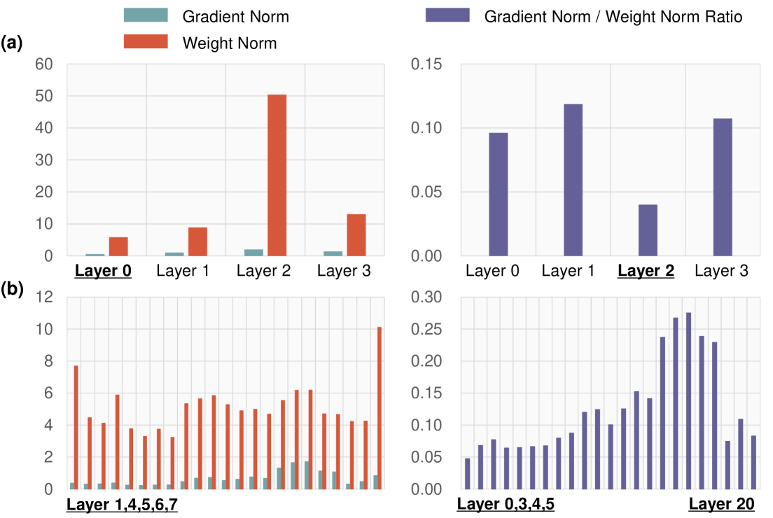
Figure 1: The layer-wise gradient norm and weight norm comparison (left) and the ratio of the gradient norm to the weight norm (right). The top-side (a) shows FEMNIST (CNN) and the bottom-side, (b) shows CIFAR-10 (ResNet20). It is clearly shown that the layers with the smallest gradients do not always least significantly affect the model parameter values.

3.1 Motivation

Many existing communication-efficient FL methods focus on how to reduce the communication cost while maintaining the gradient magnitude as similar as possible. For instance, update sparsification methods select a subset of parameters with small gradients and omit their updates Alistarh et al. (2018); Bibikar et al. (2021). Layer-wise model aggregation methods selectively aggregate the local updates at a subset of layers with small gradient norms Azam et al. (2021); Lee et al. (2023b). These methods commonly assume that larger gradients indicate greater importance.

Figure 1 shows layer-wise intermediate data collected from FEMNIST (top) and CIFAR-10 (bottom) training. The left-side chart compares the gradient norm and the weight norm while the right-side chart shows the ratio of the gradient norm to the weight norm. The IDs of a few layers with small gradient magnitudes (left) and ratios (right) are shown at the bottom of the charts. The detailed hyper-parameter settings can be found in Appendix.

The key message from this empirical study is that layers with small gradients do not necessarily show a small ratio of gradient norm to weight norm. The small ratio can be interpreted as a less significant impact of the update on changes in parameter value. Even when the gradient is large, if the corresponding parameter is also large, its effect on the layer’s output will remain minimal. From the perspective of each layer, therefore, the ratio may serve as a more critical metric than the magnitude of the gradients alone. This observation motivates us to explore a novel approach to prioritizing network layers by focusing on the ratio of gradient magnitude to weight magnitude rather than solely monitoring gradient magnitude.

Algorithm 1 Layer-wise Update Aggregation with Recycling (LUAR)

1:Input: $\Delta_{t}^{i}$: the latest local updates, $\hat{\Delta}_{t-1}$: the updates used at the previous round, $\mathcal{R}_{t}$: the set of recycling layers, $\delta$: the number of recycling layers

2:Clients send out the local updates: $\textbf{u}_{t}^{i}=[\Delta_{t,l}^{i}],\forall l\notin\mathcal{R}_{t}$

3:Server aggregates the updates: $\textbf{u}_{t}=\frac{1}{a}\sum_{i=1}^{a}\textbf{u}_{t}^{i}$

4:$\textbf{r}_{t}=[\hat{\Delta}_{t-1,l}],\forall l\in\mathcal{R}_{t}$

5:$\hat{\Delta}_{t}=[\textbf{r}_{t},\textbf{u}_{t}]$

6:Update the recycling scores: $\mathbf{s}_{t,l}$ $\triangleright$ Eq. (1)

7:$\textbf{p}^{t}\leftarrow\text{Calculate }p_{l}^{t}$, $\forall l\in[L]$ $\triangleright$ Eq. (2)

8:$\mathcal{R}_{t+1}\leftarrow$ Random_Choice($[L]$, $\delta$, $\textbf{p}^{t}$)

9:Output: $\hat{\Delta}_{t},\mathcal{R}_{t+1}$

3.2 Layer-wise Update Recycling

Gradient-Weight Ratio Analysis – We prioritize network layers using the ratio of gradient magnitude to weight magnitude. Given $L$ layers of a neural network, the prioritization metric $s_{t,l}$ is defined as follows.

$$s_{t,l}=\frac{\|\Delta_{t,l}\|}{\|\mathbf{x}_{t,l}\|},\forall l\in\{0,\cdots,L-1\}$$ (1)

where $\Delta_{t,l}$ is the accumulated local updates averaged across all the clients at round $t$ for layer $l$, and $\mathbf{x}_{t,l}$ is the initial model parameters of layer $l$ at round $t$. Intuitively, this metric quantifies the relative gradient magnitude based on parameter magnitude. If $s_{t,l}$ is measured large, we expect the layer’s parameters to move fast on the parameter space making it sensitive to the update correctness. In contrast, if $s_{t,l}$ is small, the layer’s parameters will not be dramatically changed after each update. We assign low priority to layer $l$ if its $s_{t,l}$ is small, and high priority if it is large. In this way, all the $L$ layers can be prioritized based on how actively the parameters are changed after each round.

This metric can be efficiently measured at the server-side. The $\mathbf{x}_{t,l}$ is already stored in the server before every communication round. All FL methods aggregate the local updates after every round, and thus $\Delta_{t,l}$ is also already ready to be used in the server. Therefore, $s_{t,l}$ can be easily measured without any extra communications. This is a critical advantage considering the limited network bandwidth in typical FL environments.
Layer-wise Stochastic Update Recycling Method – We design a novel FL method that recycles the previous updates for a subset of layers. The first step is to calculate a probability distribution of $L$ network layers based on the prioritization metric shown in (1). The probability of layer $l$ to be chosen is computed as follows:

$$p_{t,l}=\frac{1/s_{t,l}}{\sum_{l=0}^{L-1}1/s_{t,l}},\forall l\in\{0,\cdots,L-1\}.$$ (2)

Each layer has a weight factor $\frac{1}{s_{t,l}}$ so that it is less likely chosen if its priority is low. Dividing it by $\sum_{i=0}^{L-1}1/s_{t,l}$ ensures the sum of all weight factors equals $1$, allowing $p$ values to be directly used as weight factor of random sampling. Second, our method randomly samples $\delta$ layers using the probability distribution $\mathbf{p}$ shown in (2). We define those sampled layers at round $t$ as $\mathcal{R}_{t}$. Finally, the sampled $\delta$ layers are updated using the previous round’s updates instead of the latest updates. That is, the clients do not send the local updates for those $\delta$ layers to the server.

It is worth noting that the weighted random sampling-based layer selection prevents the updates for low-priority layers from being recycled excessively. When low-priority layers are not sampled, their updates will be normally aggregated at the server-side and thus their $s_{t,l}$ values can be updated. We will analyze the impact of this stochastic layer selection scheme on the overall performance of the update recycling method in Section 4.

Algorithm 2 Federated Learning with Layer-wise Update Aggregation with Recycling (FedLUAR)

1:Input: $a$: the number of active clients per round, $T$: the total number of rounds

2:$\mathcal{R}_{0}$ is initialized to all the layers.

3:for $t\in\{0,\cdots,T-1\}$ do

4:  $\mathcal{A}=\textrm{Random\_Choice}([\mathcal{N}],a)$.

5:  Server sends out $\textbf{x}_{t}$, $\mathcal{R}_{t}$ to the clients $\forall i\in[\mathcal{A}]$.

6:  Client receives the model: $\textbf{x}_{t,0}^{i}=\textbf{x}_{t}$.

7:  for $j\in\{1,\cdots,\tau\}$ do

8:   $\textbf{x}_{t,j}^{i}=\textrm{Local\_Update}(\textbf{x}_{t,j-1}^{i})$.

9:  end for

10:  Clients calculate the update $\Delta_{t}^{i}=\textbf{x}_{t,\tau}^{i}-\textbf{x}_{t,0}^{i}$.

11:  $\hat{\Delta}_{t},\mathcal{R}_{t+1}=\textrm{LUAR}(\Delta_{t}^{i},\hat{\Delta}_{t-1},\mathcal{R}_{t}$) $\triangleright$ Alg.1

12:  $\textbf{x}_{t+1}=\textbf{x}_{t}+\hat{\Delta}_{t}$

13:end for

14:Output: $\textbf{x}_{T}$

We formally define the update recycling method as follows.

$$\textbf{u}_{t} =[\Delta_{t,l}],\forall l\notin\mathcal{R}_{t}$$ (3)

$$\textbf{r}_{t} =[\hat{\Delta}_{t-1,l}],\forall l\in\mathcal{R}_{t}$$ (4)

$$\hat{\Delta}_{t} =[\textbf{r}_{t},\textbf{u}_{t}],$$ (5)

where ${\textbf{u}_{t}}$ is the updates for layers not included in $\mathcal{R}_{t}$, $\textbf{r}_{t}$ is the recycled updates for $\delta$ layers in $\mathcal{R}_{t}$, and $\hat{\Delta}_{t}$ is the global update composed of $\mathbf{u}_{t}$ and $\mathbf{r}_{t}$. Algorithm 1 shows Layer-wise Update Aggregation with Recycling (LUAR) method. Note that the number of layers whose update will be recycled, $\delta$, is a user-tunable hyper-parameter. We will further discuss how $\delta$ affects the model accuracy as well as the communication cost in Section 4.
Federated Learning Framework – Algorithm 2 shows FedLUAR, a FL framework built upon the proposed LUAR method shown in Algorithm 1. Before the active clients download the initial model parameters $\mathbf{x}_{t}$, the server lets them know the layers whose update will be recycled, $\mathcal{R}_{t}$ (line 5). Next, all individual clients run local training for $\tau$ iterations. Then, the local updates are aggregated using LUAR (line 11). Finally, the global model is updated using $\hat{\Delta}_{t}$. Figure 2 shows a schematic illustration of FedLUAR. If $\delta=0$, then $\hat{\Delta}_{t}$ becomes the same as $\Delta_{t}$, making it the vanilla FedAvg. In this paper, we use FedAvg as the base federated optimization algorithm for simplicity. However, extending it to more advanced FL optimizers is straightforward since LUAR is not dependent on any specific optimizer.
Potential Limitations – The proposed FL method consumes slightly increased memory space at the server-side as compared to the vanilla FedAvg. Specifically, as the server keeps $\delta$ selected layers’ previous updates, it requires a larger amount of memory space accordingly. In addition, the server should inform active clients about which layers’ updates should be omitted when transmitting the local updates to the server. This introduces only a negligible overhead, as the list of recycling layer IDs can be sent along with the initial model parameters before each communication round.

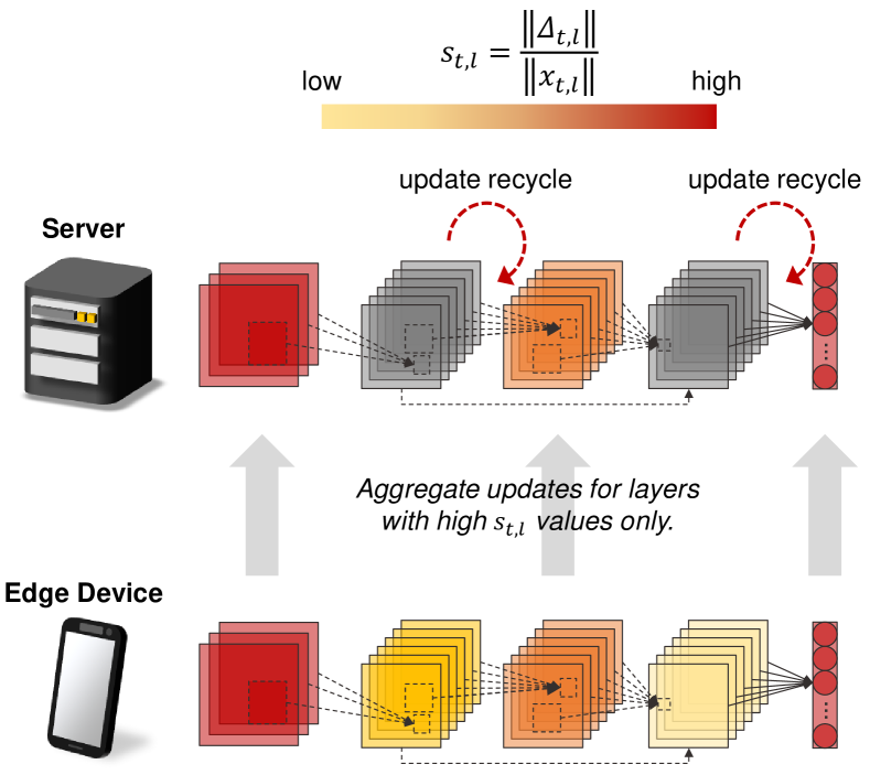
Figure 2: A schematic illustration of FedLUAR. Each client sends out updates for layers with large $s_{t,l}$ values only. For the other layers, the server ‘recycles’ the previous updates.

3.3 Theoretical Analysis

We consider non-convex and smooth optimization problems:

$$\min_{\mathbf{x}\in\mathbb{R}^{d}}F(\mathbf{x}):=\frac{1}{m}\sum_{i=1}^{m}F_{i}(\mathbf{x}),$$

where $F_{i}(\mathbf{x})=\mathbb{E}_{\xi_{i}\sim D_{i}}[f(\mathbf{x},\xi_{i})]$ is the local loss function associated with the local data distribution $D_{i}$ of client $i$ and $m$ is the number of clients.

Our analysis is based on the following assumptions.
Assumption 1. (Lipschitz continuity) There exists a constant $\mathcal{L}>0$, such that $\|\nabla F_{i}(\mathbf{x})-\nabla F_{i}(\mathbf{y})\|\leq\mathcal{L}\|\mathbf{x}-\mathbf{y}\|,\forall\mathbf{x},\mathbf{y}\in\mathbb{R}^{d},\textrm{ and }i\in[m]$.
Assumption 2. (Unbiased local gradients) The local gradient estimator is unbiased such that $\mathbb{E}_{\xi_{i}\sim D_{i}}[\nabla f(\mathbf{x},\xi_{i})]=\nabla F_{i}(\mathbf{x}),\forall i\in[m]$.
Assumption 3. (Bounded local and global variance) There exist two constants $\sigma_{L}>0$ and $\sigma_{G}>0$, such that the local gradient variance is bounded by $\mathbb{E}[\|\nabla f(\mathbf{x},\xi_{i})-\nabla F_{i}(\mathbf{x})\|]^{2}\leq\sigma_{L}^{2},\forall i\in[m]$, and the global variability is bounded by $\mathbb{E}\left[\|\nabla F_{i}(\mathbf{x})-\nabla F(\mathbf{x})\|^{2}\right]\leq\sigma_{G}^{2},\forall i\in[m]$.

We define $\hat{g}$ as a stochastic gradient vector that has zero in the selected $\delta$ layers where their updates will be recycled. Likewise, the corresponding full-batch gradient is defined as $\nabla\hat{F}(\mathbf{x})$. To analyze the impact of the update recycling in Algorithm 1, we also define the quantity of noise $n_{t}$ as follows.

$$n_{t}:=\hat{\Delta}_{t}-\Delta_{t}=\frac{1}{m}\sum_{i=1}^{m}\sum_{j=0}^{\tau-1}\left(\hat{g}_{t-k,j}^{i}-\hat{g}_{t,j}^{i}\right).$$ (6)

The $k$ in (6) represents the degree of update staleness, which increases as the update is recycled in consecutive communication rounds. As shown in Algorithm 1, our proposed method does not specify the upper bound of $k$ and adaptively selects the recycling layers based only on $s_{t,l}$ values. Therefore, we analyze the convergence rate of Algorithm 2 without any assumptions on the $k$ value.

Herein, we present our theoretical analysis on the convergence rate of Algorithm 2 (See Appendix for proofs).

Lemma 3.1.

(noise) Under assumption $1\sim 3$, if the learning rate $\eta\leq\frac{1}{\mathcal{L}\tau}$, the accumulated noise is bounded as follows.

$$\sum_{t=0}^{T-1}\mathbb{E}\left[\left\|n_{t}\right\|^{2}\right] \leq 4T\tau^{2}\sigma_{L}^{2}+8T\tau^{2}\sigma_{G}^{2}$$

$$\quad+8\kappa\tau^{2}\sum_{t=0}^{T-1}\mathbb{E}\left[\left\|\nabla F(\mathbf{x}_{t})\right\|^{2}\right]$$

$$\quad+\frac{8\tau L^{2}}{m}\sum_{t=0}^{T-1}\sum_{i=1}^{m}\sum_{j=0}^{\tau-1}\mathbb{E}\left[\left\|\mathbf{x}_{t,j}^{i}-\mathbf{x}_{t}\right\|^{2}\right],$$

where $m$ is the number of clients and $\kappa$ is the ratio of $\|\nabla\hat{F}(\mathbf{x}_{t})\|^{2}$ to $\|\nabla F(\mathbf{x}_{t})\|^{2}$ which is $\leq 1$.

Theorem 3.2.

Under assumption $1\sim 3$, if the learning rate $\eta\leq\frac{1-16\kappa}{6\sqrt{30}\mathcal{L}\tau}$ and $\kappa<\frac{1}{16}$, we have

$$\sum_{t=0}^{T-1}\mathbb{E}\left[\left\|\nabla F(\mathbf{x}_{t})\right\|^{2}\right] \leq\frac{4}{(1-16\kappa)\eta\tau}\left(F(\mathbf{x}_{0})-F(\mathbf{x}_{T})\right)$$

$$\quad+\frac{4T}{1-16\kappa}\left(\frac{\mathcal{L}\eta}{m}+4+9\mathcal{L}^{2}\right)\sigma_{L}^{2}$$ (7)

$$\quad+\frac{1080T\mathcal{L}^{2}\eta^{2}\tau^{2}}{1-16\kappa}\sigma_{G}^{2}.$$

Remark 1. Lemma 3.1 shows that the update recycling method ensures the noise magnitude bounded regardless of how many times the updates are recycled and how many layers recycle their updates if $\kappa$ is sufficiently small. This result can serve as a foundation that allows users to safely recycle updates in a layer-wise manner, thereby reducing communication costs.

Remark 2. Algorithm 2 converges to a neighbor region of a minimum since the term of $(4+9\mathcal{L}^{2})\sigma_{L}^{2}$ in (7) is not affected by the learning rate $\eta$. However, all the other terms are zeroed out as $\eta$ diminishes. Thus, we can conclude that Algorithm 2 ensures practical convergence properties in real-world applications.

Intuitively, Theorem 3.2 shows that the data heterogeneity affects how closely the model converges to a minimum. To mitigate this effect, one could use a relatively large batch size during local training steps to help the model converge as closely as possible to the minimum.

Algorithm	CIFAR-10		CIFAR-100		FEMNIST		AG News
	(ResNet20)		(WRN-28)		(CNN)		(DistillBERT)
	Accuracy	Comm	Accuracy	Comm	Accuracy	Comm	Accuracy	Comm
FedAvg	$61.27\pm 0.7\%$	$1.00$	$59.88\pm 0.8\%$	$1.00$	$71.01\pm 0.4\%$	$1.00$	$82.66\pm 0.2\%$	$1.00$
LBGM (Low-rank Approximation)	$54.87\pm 0.5\%$	$0.65$	$57.13\pm 0.2\%$	$0.87$	$69.83\pm 1.0\%$	$0.71$	$77.96\pm 0.1\%$	$0.23$
FedPAQ (Quantization)	$57.42\pm 0.2\%$	$0.50$	$36.15\pm 0.1\%$	$0.50$	$71.54\pm 0.1\%$	$0.25$	$82.72\pm 0.1\%$	$0.25$
FedPara (Re-parameterization)	$55.16\pm 0.1\%$	$0.51$	$46.14\pm 0.1\%$	$0.61$	$67.69\pm 0.1\%$	$0.22$	$75.22\pm 0.1\%$	$0.69$
PruneFL (Pruning)	$56.76\pm 0.1\%$	$0.51$	$59.40\pm 0.1\%$	$0.69$	$69.42\pm 0.4\%$	$0.19$	$77.25\pm 0.1\%$	$0.22$
FedDropoutAvg (Dropout)	$56.54\pm 0.3\%$	$0.50$	$51.25\pm 0.1\%$	$0.60$	$70.61\pm 0.1\%$	$0.25$	$64.94\pm 0.1\%$	$0.50$
FedLUAR (Proposed)	$\mathbf{60.15\pm 0.7\%}$	$\mathbf{0.47}$	$\mathbf{59.73\pm 0.6\%}$	$\mathbf{0.61}$	$\mathbf{73.17\pm 0.1\%}$	$\mathbf{0.18}$	$\mathbf{82.80\pm 0.1\%}$	$\mathbf{0.17}$

Table 1: The classification performance comparisons. The communication cost is normalized relative to that of full model averaging. The hyper-parameters are tuned to achieve comparable accuracy to FedAvg while maximizing communication cost reduction.

4 Experiments

Experimental Settings – All experiments are conducted on a GPU cluster which has 2 NVIDIA A6000 GPUs per machine. We use TensorFlow 2.15.0 for training and MPI for model aggregations. All individual experiments were performed at least 3 times, and the average accuracies are reported.

Datasets – We evaluate the performance of our proposed method on representative benchmarks: CIFAR-10 (ResNet20 He et al. (2016)), CIFAR-100 (Wide-ResNet28 Zagoruyko and Komodakis (2016)), FEMNIST (CNN), and AG News (DistillBert Sanh et al. (2019)). When tuning hyper-parameters, we conduct a grid search with a sufficiently small unit size (e.g., 0.1 for learning rate). To generate non-IID datasets, we use label-based Dirichlet distributions with $\alpha=0.1$, which indicates highly non-IID conditions.

$\delta$	CIFAR-10		CIFAR-100
	Acc. (%)	Comm.	Acc. (%)	Comm.
0	$61.27\pm 0.7\%$	$1.00$	$59.88\pm 0.8\%$	$1.00$
4	$61.25\pm 0.4\%$	$0.84$	$59.85\pm 0.1\%$	$0.88$
8	$60.92\pm 1.7\%$	$0.68$	$59.93\pm 0.1\%$	$0.76$
12	$60.15\pm 0.7\%$	$0.47$	$59.73\pm 0.6\%$	$0.61$
16	$50.07\pm 1.6\%$	$0.30$	$55.03\pm 0.7\%$	$0.51$
20	N/A	N/A	$49.60\pm 0.2\%$	$0.36$

Table 2: The CIFAR-10/100 (ResNet20/WideResNet28) classification performance with varying $\delta$ settings. The accuracy remains nearly the same until $\delta$ grows to $12$ for both datasets.

4.1 Comparative Study

We begin by presenting an accuracy comparison among SOTA communication-efficient FL methods below.

• LBGM Azam et al. (2021)

• FedPAQ Reisizadeh et al. (2020)

• FedPara Hyeon-Woo et al. (2021)

• PruneFL Jiang et al. (2022)

• FedDropoutAvg Gunesli et al. (2021)

Look-back Gradient Multiplier (LBGM) is a communication-efficient FL method which reuses the model updates in a low-rank space. FedPAQ is a quantization-based FL method that reduces the communication cost in model aggregation by quantizing all individual model parameters. FedPara is a low-rank model decomposition-based FL method which is a representative re-parameterization technique. PruneFL tackles the communication cost in FL by dropping a part of model parameters. FedDropoutAvg is a recently proposed FL method that allows each client to randomly drop the parameters at every round.

Table 1 shows the performance comparison (See Appendix). The total number of clients is 128 and randomly chosen 32 clients participate in every communication round. To make fair comparisons, we find algorithm-specific settings that achieve accuracy reasonably close to the baseline (FedAvg) while minimizing communication costs, and then directly compare the validation accuracy across algorithms.

Overall, FedLUAR achieves accuracy comparable to the baseline while significantly reducing communication costs across all four benchmarks. Particularly for FEMNIST and AG News, our method achieves nearly the same accuracy as FedAvg reducing communication cost to less than $20\%$. Additionally, our proposed method outperforms all the other SOTA methods. Regardless of the dataset, FedLUAR consistently achieves the best accuracy among all the communication-efficient FL methods while having a remarkably reduced communication cost. These results clearly demonstrate that the proposed LUAR method effectively identifies the least critical layers and enables the recycling of previous updates, thereby minimizing communication costs while maintaining model accuracy.

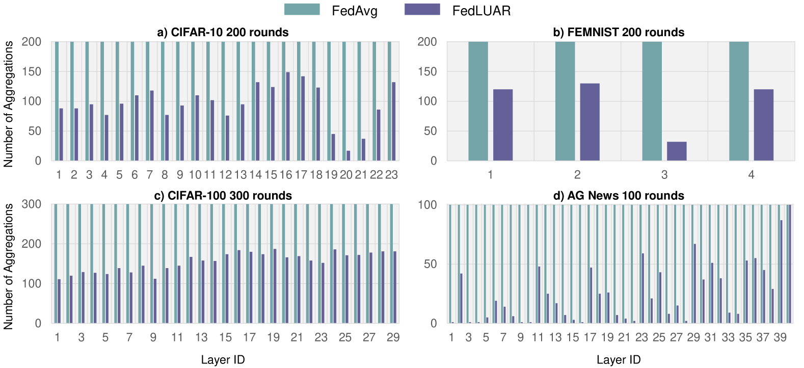
Figure 3: The number of model aggregations per layer. In all the benchmarks, FedLUAR dramatically reduces the number of model aggregations in each layer. The difference between the FedAvg count and the FedLUAR count shows how many times the updates were recycled (how many communications were skipped).

4.2 Harmonization with Other FL Methods

The proposed FL method does not have any dependencies on local training algorithms. To demonstrate this, we apply LUAR to advanced FL algorithms including FedProx Li et al. (2020), MOON Qinbin Li (2021), FedOpt Reddi et al. (2021), FedMut Hu et al. (2024), and FedACG Geeho Kim (2024), and analyze its impact on model accuracy. Table 4 shows FEMNIST accuracy comparisons (See Appendix for the detailed settings). LUAR maintains the validation accuracy while significantly reducing the communication cost across all three benchmarks. Note that the Comm values are communication cost relative to the full model averaging cost. For example, FedPAQ reduces the communication cost to $50\%$ compared to FedAvg, and LUAR further reduces it to $22\%$ of FedPAQ’s communication cost, which results in $11\%$ of FedAvg’s cost. However, LUAR barely affects the accuracy, achieving comparable accuracy to the periodic averaging. These results demonstrate that the proposed method can complement advanced FL methods and be readily applied to many real-world FL applications.

	Periodic Averaging	LUAR (Proposed)	Comm	$\delta$
FedAvg	$61.27\pm 0.1\%$	$60.97\pm 0.1\%$	$0.57$	10
FedProx	$61.74\pm 0.1\%$	$61.20\pm 0.1\%$	$0.54$
FedPAQ	$57.42\pm 0.2\%$	$57.40\pm 0.2\%$	$0.33$
FedOpt	$62.42\pm 0.1\%$	$62.28\pm 0.2\%$	$0.50$
MOON	$62.33\pm 1.2\%$	$61.65\pm 0.1\%$	$0.51$
FedMut	$61.27\pm 0.1\%$	$60.42\pm 0.1\%$	$0.56$
FedACG	$65.02\pm 0.1\%$	$64.28\pm 0.1\%$	$0.55$

Table 3: The CIFAR10 performance comparison between before and after applying LUAR to a half layers in ResNet20. LUAR remarkably reduces the communication cost while maintaining the accuracy.

	Periodic Averaging	LUAR (Proposed)	Comm	$\delta$
FedAvg	$71.01\pm 0.4\%$	$73.17\pm 0.1\%$	$0.18$	2
FedProx	$71.94\pm 0.1\%$	$73.45\pm 0.1\%$	$0.09$
FedPAQ	$71.54\pm 0.1\%$	$71.15\pm 0.1\%$	$0.11$
FedOpt	$72.34\pm 0.1\%$	$71.91\pm 0.1\%$	$0.22$
MOON	$71.55\pm 0.1\%$	$71.63\pm 0.1\%$	$0.24$
FedMut	$71.91\pm 0.1\%$	$72.31\pm 0.1\%$	$0.26$
FedACG	$72.16\pm 0.1\%$	$71.94\pm 0.1\%$	$0.21$

Table 4: The FEMNIST performance comparison between before and after applying LUAR. The communication cost is the ratio of LUAR’s cost to the periodic full averaging cost. The CNN model contains 4 layers in total, and $\delta$ is set to a half of them. For all FL methods, LUAR effectively reduces the communication cost while maintaining the validation accuracy.

4.3 Communication Cost Analysis

FedLUAR allows clients to skip sending updates for less important layers to the server, thereby reducing communication costs. Figure 3 shows the number of communications for each layer. The more frequently the updates are recycled, the lower the communication cost will be. The communication count charts demonstrate that FedLUAR performs significantly fewer communications than the vanilla FedAvg while achieving nearly the same model accuracy. One intriguing observation is that, in FEMNIST and AG News, the layer with the largest number of parameters is recycled the most, leading to a significant reduction in total communication cost. However, this trend is not observed in the CIFAR-10 and CIFAR-100 benchmarks. Thus, we can conclude that our proposed algorithm is independent of layer size or specific model architectures, adaptively identifying the least significant layers regardless of the model design.

4.4 Additional Performance Analysis

How much does it accelerate? – Figure 4 shows CIFAR-10 learning curves. The x-axis is a relative communication cost to FedAvg. To highlight the difference clearly, we selectively present comparisons among four methods only. The comparison clearly shows that FedLUAR achieves similar accuracy to FedAvg much faster than other SOTA communication-efficient FL methods. Since our method incurs little to no additional computational cost, the same performance gain can be expected in terms of the end-to-end training time in realistic FL environments. See Appendix for more curve charts.
How much could be recycled safely? – We also investigate the impact of $\delta$ on the model accuracy as well as the communication cost. We divide the number of model aggregations at each layer by the total number of communication rounds to calculate the layer-wise communication cost. Then, we sum up the calculated layer-wise costs to get the total communication cost. Intuitively, the larger the $\delta$, the lower the communication cost. However, the model accuracy is expected to drop as more layers recycle their updates.

Table 2 shows CIFAR-10 and CIFAR-100 experimental results for various $\delta$ settings. One key observation is that the accuracy is almost not degraded when LUAR is applied with $\delta\leq 12$ for both datasets. This means that many network layers have quite stable gradient dynamics, and thus their updates can be safely recycled. In addition, the accuracy is hardly reduced until the communication cost is reduced by almost $50\%$. This is a significant benefit especially in FL environments where the network bandwidth is extremely limited. See Appendix for other benchmark results.

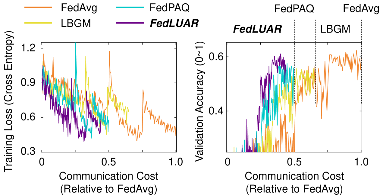
Figure 4: The learning curve comparisons for CIFAR-10 (ResNet20). The x-axis represents the communication cost relative to FedAvg. To highlight the differences clearly, we selectively present comparisons among four different methods only.

5 Conclusion

In this paper, we demonstrated that selectively recycling updates in specific layers can reduce communication costs in FL while preserving model accuracy. In particular, our study empirically proved that the gradient-to-weight magnitude ratio can serve as a practical metric for identifying the least significant layers. This layer-wise partial model aggregation scheme is expected to facilitate the development of efficient FL applications and promote the partial model training paradigm across various deep learning fields. We consider developing a communication-efficient Large Language Model fine-tuning method based on the update recycling scheme as a promising direction for future work.

Appendix A Appendix

A.1 Theoretical Analysis

We consider non-convex and smooth optimization problems as follows.

$$\min_{x\in\mathbb{R}^{d}}F(x):=\frac{1}{m}\sum_{i=1}^{m}F_{i}(x),$$ (8)

where $F_{i}(x)=\mathbb{E}_{\xi_{i}\sim D_{i}}[f(x,\xi_{i})]$ is the local loss function associated with the local data distribution $D_{i}$ of client $i$ and $m$ is the number of clients.

Our analysis is based on the following assumptions.

Assumption 1. (Lipschitz continuity) There exists a constant $\mathcal{L}>0$, such that $\|\nabla F_{i}(x)-\nabla F_{i}(y)\|\leq\mathcal{L}\|x-y\|,\forall x,y\in\mathbb{R}^{d},\mathrm{and}i\in[m]$.

Assumption 2. (Unbiased local gradients) The local gradient estimator is unbiased such that $\mathbb{E}_{\xi_{i}\sim D_{i}}[\nabla f(x,\xi_{i})]=\nabla F_{i}(x),\forall i\in[m]$.

Assumption 3. (Bounded local and global variance) There exist two constants $\sigma_{L}>0$ and $\sigma_{G}>0$, such that the local gradient variance is bounded by $\mathbb{E}[\|\nabla f(x,\xi_{i})-\nabla F_{i}(x)\|]^{2}\leq\sigma_{L}^{2},\forall i\in[m]$, and the global variability is bounded by $\mathbb{E}\left[\|\nabla F_{i}(x)-\nabla F(x)\|^{2}\right]\leq\sigma_{G}^{2},\forall i\in[m]$.

Herein, we analyze the convergence properties of FedAvg as follows. First, the following Lemma is a slightly refined version of Lemma 3 in Reddi et al. [2021]. This Lemma is also used as Lemma 2 in Yang et al. [2021].

Lemma A.1.

(model discrepancy) For any step-size satisfying $\eta\leq\frac{1}{2\sqrt{3}L\tau}$, we have the following result:

$$\frac{1}{m}\sum_{i=0}^{m}\mathbb{E}[\|\mathbf{x}_{t,k}^{i}-\mathbf{x}_{t}\|^{2}] \leq 5\eta^{2}\sigma_{L}^{2}+30\tau\eta^{2}\sigma_{G}^{2}+30\tau\eta^{2}\mathbb{E}[\|\nabla F(\mathbf{x}_{t})\|^{2}].$$

Proof.

For any client $i\in[m]$, $t\in[T-1]$, and $k\in[\tau]$, we have

$$\mathbb{E}[\|\mathbf{x}_{t,k}^{i}-\mathbf{x}_{t}\|^{2}]=\mathbb{E}[\|\mathbf{x}_{t,k-1}^{i}-\mathbf{x}_{t}-\eta g_{t,k-1}^{i}\|^{2}]$$

$$=\mathbb{E}[\|\mathbf{x}_{t,k-1}^{i}-\mathbf{x}_{t}-\eta\left(g_{t,k-1}^{i}-\nabla F_{i}(\mathbf{x}_{t,k-1}^{i})+\nabla F_{i}(\mathbf{x}_{t,k-1}^{i})-\nabla F_{i}(\mathbf{x}_{t})+\nabla F_{i}(\mathbf{x}_{t})-\nabla F(\mathbf{x}_{t})+\nabla F(\mathbf{x}_{t})\right)\|^{2}]$$

$$=\mathbb{E}[\|\eta\left(g_{t,k-1}^{i}-\nabla F_{i}(\mathbf{x}_{t,k-1}^{i})\right)\|^{2}]$$

$$\quad+2\mathbb{E}[\langle\eta\left(g_{t,k-1}^{i}-\nabla F_{i}(\mathbf{x}_{t,k-1}^{i})\right),\mathbf{x}_{t,k-1}^{i}-\mathbf{x}_{t}-\eta\left(\nabla F_{i}(\mathbf{x}_{t,k-1}^{i})-\nabla F_{i}(\mathbf{x}_{t})+\nabla F_{i}(\mathbf{x}_{t})-\nabla F(\mathbf{x}_{t})+\nabla F(\mathbf{x}_{t})\right)\rangle]$$

$$\quad+\mathbb{E}[\|\mathbf{x}_{t,k-1}^{i}-\mathbf{x}_{t}-\eta\left(\nabla F_{i}(\mathbf{x}_{t,k-1}^{i})-\nabla F_{i}(\mathbf{x}_{t})+\nabla F_{i}(\mathbf{x}_{t})-\nabla F(\mathbf{x}_{t})+\nabla F(\mathbf{x}_{t})\right)\|^{2}]$$

$$=\mathbb{E}[\|\eta\left(g_{t,k-1}^{i}-\nabla F_{i}(\mathbf{x}_{t,k-1}^{i})\right)\|^{2}]$$ (9)

$$\quad+\mathbb{E}[\|\mathbf{x}_{t,k-1}^{i}-\mathbf{x}_{t}-\eta\left(\nabla F_{i}(\mathbf{x}_{t,k-1}^{i})-\nabla F_{i}(\mathbf{x}_{t})+\nabla F_{i}(\mathbf{x}_{t})-\nabla F(\mathbf{x}_{t})+\nabla F(\mathbf{x}_{t})\right)\|^{2}]$$

$$\leq\eta^{2}\sigma_{L}^{2}+\mathbb{E}[\|\mathbf{x}_{t,k-1}^{i}-\mathbf{x}_{t}-\eta\left(\nabla F_{i}(\mathbf{x}_{t,k-1}^{i})-\nabla F_{i}(\mathbf{x}_{t})+\nabla F_{i}(\mathbf{x}_{t})-\nabla F(\mathbf{x}_{t})+\nabla F(\mathbf{x}_{t})\right)\|^{2}]$$

$$\leq\eta^{2}\sigma_{L}^{2}+\left(1+\frac{1}{2\tau-1}\right)\mathbb{E}[\|\mathbf{x}_{t,k-1}^{i}-\mathbf{x}_{t}\|^{2}]$$ (10)

$$\quad+2\tau\eta^{2}\mathbb{E}[\|\nabla F_{i}(\mathbf{x}_{t,k-1}^{i})-\nabla F_{i}(\mathbf{x}_{t})+\nabla F_{i}(\mathbf{x}_{t})-\nabla F(\mathbf{x}_{t})+\nabla F(\mathbf{x}_{t})\|^{2}]$$

$$\leq\eta^{2}\sigma_{L}^{2}+\left(1+\frac{1}{2\tau-1}\right)\mathbb{E}[\|\mathbf{x}_{t,k-1}^{i}-\mathbf{x}_{t}\|^{2}]$$

$$\quad+6\tau\eta^{2}\left(\mathbb{E}[\|\nabla F_{i}(\mathbf{x}_{t,k-1}^{i})-\nabla F_{i}(\mathbf{x}_{t})\|^{2}]+\mathbb{E}[\|\nabla F_{i}(\mathbf{x}_{t})-\nabla F(\mathbf{x}_{t})\|^{2}]+\mathbb{E}[\|\nabla F(\mathbf{x}_{t})\|^{2}]\right)$$

$$\leq\eta^{2}\sigma_{L}^{2}+\left(1+\frac{1}{2\tau-1}\right)\mathbb{E}[\|\mathbf{x}_{t,k-1}^{i}-\mathbf{x}_{t}\|^{2}]$$

$$\quad+6\tau\eta^{2}\sigma_{G}^{2}+6\tau\eta^{2}L^{2}\mathbb{E}[\|\mathbf{x}_{t,k-1}^{i}-\mathbf{x}_{t}\|^{2}]+6\tau\eta^{2}\mathbb{E}[\|\nabla F(\mathbf{x}_{t})\|^{2}]$$

$$=\eta^{2}\sigma_{L}^{2}+6\tau\eta^{2}\sigma_{G}^{2}+\left(1+\frac{1}{2\tau-1}+6\tau\eta^{2}L^{2}\right)\mathbb{E}[\|\mathbf{x}_{t,k-1}^{i}-\mathbf{x}_{t}\|^{2}]+6\tau\eta^{2}\mathbb{E}[\|\nabla F(\mathbf{x}_{t})\|^{2}],$$

where (9) is because $\mathbb{E}[g_{t,k-1}^{i}]=\nabla F_{i}(\mathbf{x}_{t,k}^{i})$. The (10) is based on the fact that

$$\|\mathbf{a}+\mathbf{b}\|^{2}\leq(1+\frac{1}{\alpha})\|\mathbf{a}\|^{2}+(1+\alpha)\|\mathbf{b}\|^{2}$$

for any $\alpha>0$.

Next, if $\eta\leq\frac{1}{2\sqrt{3}L\tau}$, the above bound can be simplified as follows.

$$\mathbb{E}[\|\mathbf{x}_{t,k}^{i}-\mathbf{x}_{t}\|^{2}]$$

$$\leq\eta^{2}\sigma_{L}^{2}+6\tau\eta^{2}\sigma_{G}^{2}+\left(1+\frac{1}{2\tau-1}+6\tau\eta^{2}L^{2}\right)\mathbb{E}[\|\mathbf{x}_{t,k-1}^{i}-\mathbf{x}_{t}\|^{2}]+6\tau\eta^{2}\mathbb{E}[\|\nabla F(\mathbf{x}_{t})\|^{2}]$$

$$\leq\eta^{2}\sigma_{L}^{2}+6\tau\eta^{2}\sigma_{G}^{2}+\left(1+\frac{1}{\tau-1}\right)\mathbb{E}[\|\mathbf{x}_{t,k-1}^{i}-\mathbf{x}_{t}\|^{2}]+6\tau\eta^{2}\mathbb{E}[\|\nabla F(\mathbf{x}_{t})\|^{2}].$$

Then, by unrolling the recursion until $k-1$ goes to $0$, we have

$$\mathbb{E}[\|\mathbf{x}_{t,k}^{i}-\mathbf{x}_{t}\|^{2}] \leq\sum_{j=0}^{k-1}\left(1+\frac{1}{\tau-1}\right)^{j}\left(\eta^{2}\sigma_{L}^{2}+6\tau\eta^{2}\sigma_{G}^{2}+6\tau\eta^{2}\mathbb{E}[\|\nabla F(\mathbf{x}_{t})\|^{2}]\right)$$

$$\leq(\tau-1)((1+\frac{1}{\tau-1})^{k-1}-1)\left(\eta^{2}\sigma_{L}^{2}+6\tau\eta^{2}\sigma_{G}^{2}+6\tau\eta^{2}\mathbb{E}[\|\nabla F(\mathbf{x}_{t})\|^{2}]\right)$$

$$\leq(\tau-1)((1+\frac{1}{\tau-1})^{\tau}-1)\left(\eta^{2}\sigma_{L}^{2}+6\tau\eta^{2}\sigma_{G}^{2}+6\tau\eta^{2}\mathbb{E}[\|\nabla F(\mathbf{x}_{t})\|^{2}]\right)$$

$$\leq 5\tau\eta^{2}\sigma_{L}^{2}+30\tau^{2}\eta^{2}\sigma_{G}^{2}+30\tau^{2}\eta^{2}\mathbb{E}[\|\nabla F(\mathbf{x}_{t})\|^{2}].$$ (11)

where (11) is because that the maximum value of $(\tau-1)((1+\frac{1}{\tau-1})^{\tau}-1)$ is $\frac{19}{4}$ when $\tau=3$. Finally, because the right-hand side of (11) is independent of $m$, we have

$$\frac{1}{m}\sum_{i=0}^{m}\mathbb{E}[\|\mathbf{x}_{t,k}^{i}-\mathbf{x}_{t}\|^{2}] \leq 5\tau\eta^{2}\sigma_{L}^{2}+30\tau^{2}\eta^{2}\sigma_{G}^{2}+30\tau^{2}\eta^{2}\mathbb{E}[\|\nabla F(\mathbf{x}_{t})\|^{2}].$$

∎

Based on the proposed update recycling method, the noise $n_{t}$ is defined as follows.

$$n_{t}=\frac{1}{m}\sum_{i=1}^{m}\sum_{j=0}^{\tau-1}\left(\hat{g}_{t-k,j}^{i}-\hat{g}_{t,j}^{i}\right),$$

where $\hat{g}$ indicates the gradient vector that has non-zero gradients only at the layers where their updates will be recycled.

Lemma A.2.

(noise) Under assumption $1\sim 3$, if the learning rate $\eta\leq\frac{1}{\mathcal{L}\tau}$, the accumulated noise is bounded as follows.

$$\sum_{t=0}^{T-1}\mathbb{E}\left[\left\|n_{t}\right\|^{2}\right]\leq 4T\tau^{2}\sigma_{L}^{2}+8T\tau^{2}\sigma_{G}^{2}+8\kappa\tau^{2}\sum_{t=0}^{T-1}\mathbb{E}\left[\left\|\nabla F(\mathbf{x}_{t})\right\|^{2}\right]+\frac{8\tau L^{2}}{m}\sum_{t=0}^{T-1}\sum_{i=1}^{m}\sum_{j=0}^{\tau-1}\mathbb{E}\left[\left\|\mathbf{x}_{t,j}^{i}-\mathbf{x}_{t}\right\|^{2}\right],$$ (12)

where $\kappa$ is the ratio of $\|\nabla\hat{F}(\mathbf{x}_{t})\|^{2}$ to $\|\nabla F(\mathbf{x}_{t})\|^{2}$.

Proof.

$$\mathbb{E}\left[\left\|n_{t}\right\|^{2}\right] =\mathbb{E}\left[\left\|\frac{1}{m}\sum_{i=1}^{m}\sum_{j=0}^{\tau-1}\left(\hat{g}_{t-k,j}^{i}-\hat{g}_{t,j}^{i}\right)\right\|^{2}\right]$$

$$\leq 2\mathbb{E}\left[\left\|\frac{1}{m}\sum_{i=1}^{m}\sum_{j=0}^{\tau-1}\hat{g}_{t-k,j}^{i}\right\|^{2}\right]+2\mathbb{E}\left[\left\|\frac{1}{m}\sum_{i=1}^{m}\sum_{j=0}^{\tau-1}\hat{g}_{t,j}^{i}\right\|^{2}\right]$$

$$\leq\frac{2\tau}{m}\sum_{i=1}^{m}\sum_{j=0}^{\tau-1}\mathbb{E}\left[\left\|\hat{g}_{t-k,j}^{i}\right\|^{2}\right]+\frac{2\tau}{m}\sum_{i=1}^{m}\sum_{j=0}^{\tau-1}\mathbb{E}\left[\left\|\hat{g}_{t,j}^{i}\right\|^{2}\right]$$

$$=\frac{2\tau}{m}\sum_{i=1}^{m}\sum_{j=0}^{\tau-1}\mathbb{E}\left[\left\|\hat{g}_{t-k,j}^{i}-\nabla\hat{F}_{i}(\mathbf{x}_{t-k,j}^{i})+\nabla\hat{F}_{i}(\mathbf{x}_{t-k,j}^{i})\right\|^{2}\right]$$

$$\quad+\frac{2\tau}{m}\sum_{i=1}^{m}\sum_{j=0}^{\tau-1}\mathbb{E}\left[\left\|\hat{g}_{t,j}^{i}-\nabla\hat{F}_{i}(\mathbf{x}_{t,j}^{i})+\nabla\hat{F}_{i}(\mathbf{x}_{t,j}^{i})\right\|^{2}\right]$$

$$=\frac{2\tau}{m}\sum_{i=1}^{m}\sum_{j=0}^{\tau-1}\left(\mathbb{E}\left[\left\|\hat{g}_{t-k,j}^{i}-\nabla\hat{F}_{i}(\mathbf{x}_{t-k,j}^{i})\right\|^{2}\right]+\mathbb{E}\left[\left\|\nabla\hat{F}_{i}(\mathbf{x}_{t-k,j}^{i})\right\|^{2}\right]\right)$$ (13)

$$\quad+\frac{2\tau}{m}\sum_{i=1}^{m}\sum_{j=0}^{\tau-1}\left(\mathbb{E}\left[\left\|\hat{g}_{t,j}^{i}-\nabla\hat{F}_{i}(\mathbf{x}_{t,j}^{i})\right\|^{2}\right]+\mathbb{E}\left[\left\|\nabla\hat{F}_{i}(\mathbf{x}_{t,j}^{i})\right\|^{2}\right]\right)$$

$$\leq 2\tau^{2}\sigma_{L}^{2}+\frac{2\tau}{m}\sum_{i=1}^{m}\sum_{j=0}^{\tau-1}\mathbb{E}\left[\left\|\nabla\hat{F}_{i}(\mathbf{x}_{t-k,j}^{i})\right\|^{2}\right]+2\tau^{2}\sigma_{L}^{2}+\frac{2\tau}{m}\sum_{i=1}^{m}\sum_{j=0}^{\tau-1}\mathbb{E}\left[\left\|\nabla\hat{F}_{i}(\mathbf{x}_{t,j}^{i})\right\|^{2}\right].$$

where (13) is based on the fact that $\mathbb{E}[\|\mathbf{x}\|^{2}]=\mathbb{E}[\|\mathbf{x}-\mathbb{E}[\mathbf{x}]\|^{2}]+\|\mathbb{E}[\mathbf{x}]\|^{2}$. Then, the right-hand side can be further bounded as follows.

$$\mathbb{E}\left[\left\|n_{t}\right\|^{2}\right] \leq 4\tau^{2}\sigma_{L}^{2}+\frac{2\tau}{m}\sum_{i=1}^{m}\sum_{j=0}^{\tau-1}\mathbb{E}\left[\left\|\nabla\hat{F}_{i}(\mathbf{x}_{t-k,j}^{i})\right\|^{2}\right]+\frac{2\tau}{m}\sum_{i=1}^{m}\sum_{j=0}^{\tau-1}\mathbb{E}\left[\left\|\nabla\hat{F}_{i}(\mathbf{x}_{t,j}^{i})\right\|^{2}\right]$$

$$=4\tau^{2}\sigma_{L}^{2}+\frac{2\tau}{m}\sum_{i=1}^{m}\sum_{j=0}^{\tau-1}\mathbb{E}\left[\left\|\nabla\hat{F}_{i}(\mathbf{x}_{t-k,j}^{i})-\nabla\hat{F}_{i}(\mathbf{x}_{t-k})+\nabla\hat{F}_{i}(\mathbf{x}_{t-k})\right\|^{2}\right]$$

$$\quad+\frac{2\tau}{m}\sum_{i=1}^{m}\sum_{j=0}^{\tau-1}\mathbb{E}\left[\left\|\nabla\hat{F}_{i}(\mathbf{x}_{t,j}^{i})-\nabla\hat{F}_{i}(\mathbf{x}_{t})+\nabla\hat{F}_{i}(\mathbf{x}_{t})\right\|^{2}\right]$$

$$\leq 4\tau^{2}\sigma_{L}^{2}+\frac{4\tau}{m}\sum_{i=1}^{m}\sum_{j=0}^{\tau-1}\mathbb{E}\left[\left\|\nabla\hat{F}_{i}(\mathbf{x}_{t-k,j}^{i})-\nabla\hat{F}_{i}(\mathbf{x}_{t-k})\right\|^{2}\right]+\frac{4\tau}{m}\sum_{i=1}^{m}\sum_{j=0}^{\tau-1}\mathbb{E}\left[\left\|\nabla\hat{F}_{i}(\mathbf{x}_{t-k})\right\|^{2}\right]$$

$$\quad+\frac{4\tau}{m}\sum_{i=1}^{m}\sum_{j=0}^{\tau-1}\mathbb{E}\left[\left\|\nabla\hat{F}_{i}(\mathbf{x}_{t,j}^{i})-\nabla\hat{F}_{i}(\mathbf{x}_{t})\right\|^{2}\right]+\frac{4\tau}{m}\sum_{i=1}^{m}\sum_{j=0}^{\tau-1}\mathbb{E}\left[\left\|\nabla\hat{F}_{i}(\mathbf{x}_{t})\right\|^{2}\right]$$

$$\leq 4\tau^{2}\sigma_{L}^{2}+\frac{4\tau L^{2}}{m}\sum_{i=1}^{m}\sum_{j=0}^{\tau-1}\mathbb{E}\left[\left\|\mathbf{x}_{t-k,j}^{i}-\mathbf{x}_{t-k}\right\|^{2}\right]+\frac{4\tau}{m}\sum_{i=1}^{m}\sum_{j=0}^{\tau-1}\mathbb{E}\left[\left\|\nabla\hat{F}_{i}(\mathbf{x}_{t-k})\right\|^{2}\right]$$

$$\quad+\frac{4\tau L^{2}}{m}\sum_{i=1}^{m}\sum_{j=0}^{\tau-1}\mathbb{E}\left[\left\|\mathbf{x}_{t,j}^{i}-\mathbf{x}_{t}\right\|^{2}\right]+\frac{4\tau}{m}\sum_{i=1}^{m}\sum_{j=0}^{\tau-1}\mathbb{E}\left[\left\|\nabla\hat{F}_{i}(\mathbf{x}_{t})\right\|^{2}\right]$$

$$=4\tau^{2}\sigma_{L}^{2}+\frac{4\tau L^{2}}{m}\sum_{i=1}^{m}\sum_{j=0}^{\tau-1}\mathbb{E}\left[\left\|\mathbf{x}_{t-k,j}^{i}-\mathbf{x}_{t-k}\right\|^{2}\right]+\frac{4\tau L^{2}}{m}\sum_{i=1}^{m}\sum_{j=0}^{\tau-1}\mathbb{E}\left[\left\|\mathbf{x}_{t,j}^{i}-\mathbf{x}_{t}\right\|^{2}\right]$$

$$\quad+\frac{4\tau}{m}\sum_{i=1}^{m}\sum_{j=0}^{\tau-1}\mathbb{E}\left[\left\|\nabla\hat{F}_{i}(\mathbf{x}_{t-k})-\nabla\hat{F}(\mathbf{x}_{t-k})+\nabla\hat{F}(\mathbf{x}_{t-k})\right\|^{2}\right]$$

$$\quad+\frac{4\tau}{m}\sum_{i=1}^{m}\sum_{j=0}^{\tau-1}\mathbb{E}\left[\left\|\nabla\hat{F}_{i}(\mathbf{x}_{t})-\nabla\hat{F}(\mathbf{x}_{t})+\nabla\hat{F}(\mathbf{x}_{t})\right\|^{2}\right]$$

$$\leq 4\tau^{2}\sigma_{L}^{2}+\frac{4\tau L^{2}}{m}\sum_{i=1}^{m}\sum_{j=0}^{\tau-1}\mathbb{E}\left[\left\|\mathbf{x}_{t-k,j}^{i}-\mathbf{x}_{t-k}\right\|^{2}\right]+\frac{4\tau L^{2}}{m}\sum_{i=1}^{m}\sum_{j=0}^{\tau-1}\mathbb{E}\left[\left\|\mathbf{x}_{t,j}^{i}-\mathbf{x}_{t}\right\|^{2}\right]$$

$$\quad+\frac{4\tau}{m}\sum_{i=1}^{m}\sum_{j=0}^{\tau-1}\mathbb{E}\left[\left\|\nabla\hat{F}_{i}(\mathbf{x}_{t-k})-\nabla\hat{F}(\mathbf{x}_{t-k})\right\|^{2}\right]+\frac{4\tau}{m}\sum_{i=1}^{m}\sum_{j=0}^{\tau-1}\mathbb{E}\left[\left\|\nabla\hat{F}(\mathbf{x}_{t-k})\right\|^{2}\right]$$

$$\quad+\frac{4\tau}{m}\sum_{i=1}^{m}\sum_{j=0}^{\tau-1}\mathbb{E}\left[\left\|\nabla\hat{F}_{i}(\mathbf{x}_{t})-\nabla\hat{F}(\mathbf{x}_{t})\right\|^{2}\right]+\frac{4\tau}{m}\sum_{i=1}^{m}\sum_{j=0}^{\tau-1}\mathbb{E}\left[\left\|\nabla\hat{F}(\mathbf{x}_{t})\right\|^{2}\right]$$

$$=4\tau^{2}\sigma_{L}^{2}+8\tau^{2}\sigma_{G}^{2}+4\tau^{2}\mathbb{E}\left[\left\|\nabla\hat{F}(\mathbf{x}_{t-k})\right\|^{2}\right]+4\tau^{2}\mathbb{E}\left[\left\|\nabla\hat{F}(\mathbf{x}_{t})\right\|^{2}\right]$$ (14)

$$\quad+\frac{4\tau L^{2}}{m}\sum_{i=1}^{m}\sum_{j=0}^{\tau-1}\mathbb{E}\left[\left\|\mathbf{x}_{t-k,j}^{i}-\mathbf{x}_{t-k}\right\|^{2}\right]+\frac{4\tau L^{2}}{m}\sum_{i=1}^{m}\sum_{j=0}^{\tau-1}\mathbb{E}\left[\left\|\mathbf{x}_{t,j}^{i}-\mathbf{x}_{t}\right\|^{2}\right],$$

where (14) follows $\|\nabla\hat{F}(\cdot)\|^{2}\leq\|\nabla F(\cdot)\|^{2}$. By summing up $\mathbb{E}[\|n_{t}\|^{2}]$ across $T$ rounds, we have

$$\sum_{t=0}^{T-1}\mathbb{E}\left[\left\|n_{t}\right\|^{2}\right] \leq 4T\tau^{2}\sigma_{L}^{2}+8T\tau^{2}\sigma_{G}^{2}+4\tau^{2}\sum_{t=0}^{T-1}\mathbb{E}\left[\left\|\nabla\hat{F}(\mathbf{x}_{t-k})\right\|^{2}\right]+4\tau^{2}\sum_{t=0}^{T-1}\mathbb{E}\left[\left\|\nabla\hat{F}(\mathbf{x}_{t})\right\|^{2}\right]$$

$$\quad+\frac{4\tau L^{2}}{m}\sum_{t=0}^{T-1}\sum_{i=1}^{m}\sum_{j=0}^{\tau-1}\mathbb{E}\left[\left\|\mathbf{x}_{t-k,j}^{i}-\mathbf{x}_{t-k}\right\|^{2}\right]+\frac{4\tau L^{2}}{m}\sum_{t=0}^{T-1}\sum_{i=1}^{m}\sum_{j=0}^{\tau-1}\mathbb{E}\left[\left\|\mathbf{x}_{t,j}^{i}-\mathbf{x}_{t}\right\|^{2}\right]$$

$$\leq 4T\tau^{2}\sigma_{L}^{2}+8T\tau^{2}\sigma_{G}^{2}+8\tau^{2}\sum_{t=0}^{T-1}\mathbb{E}\left[\left\|\nabla\hat{F}(\mathbf{x}_{t})\right\|^{2}\right]+\frac{8\tau L^{2}}{m}\sum_{t=0}^{T-1}\sum_{i=1}^{m}\sum_{j=0}^{\tau-1}\mathbb{E}\left[\left\|\mathbf{x}_{t,j}^{i}-\mathbf{x}_{t}\right\|^{2}\right]$$

$$\leq 4T\tau^{2}\sigma_{L}^{2}+8T\tau^{2}\sigma_{G}^{2}+8\kappa\tau^{2}\sum_{t=0}^{T-1}\mathbb{E}\left[\left\|\nabla F(\mathbf{x}_{t})\right\|^{2}\right]+\frac{8\tau L^{2}}{m}\sum_{t=0}^{T-1}\sum_{i=1}^{m}\sum_{j=0}^{\tau-1}\mathbb{E}\left[\left\|\mathbf{x}_{t,j}^{i}-\mathbf{x}_{t}\right\|^{2}\right],$$

where $\kappa$ is the ratio of the recycled update norm to the full update norm. Because all the gradients at the layers not recycled are zeroed out, the ratio $\kappa$ lies between 0 and 1; $0<\kappa<1$. ∎

Lemma A.3.

(framework) Under assumption 1 $\sim$ 3, if the learning rate $\eta\leq\frac{1}{\mathcal{L}\tau}$, we have

$$\sum_{t=0}^{T-1}\mathbb{E}\left[\left\|\nabla F(\mathbf{x}_{t})\right\|^{2}\right] \leq\frac{2}{(1-16\kappa)\eta\tau}\left(F(\mathbf{x}_{0})-F(\mathbf{x}_{T})\right)+\frac{2T}{1-16\kappa}\left(\frac{\mathcal{L}\eta}{m}+4\right)\sigma_{L}^{2}+\frac{16T}{1-16\kappa}\sigma_{G}^{2}$$

$$\quad+\frac{18\mathcal{L}^{2}}{(1-16\kappa)m\tau}\sum_{t=0}^{T-1}\sum_{i=1}^{m}\sum_{j=0}^{\tau-1}\mathbb{E}\left[\left\|\mathbf{x}_{t,j}^{i}-\mathbf{x}_{t}\right\|^{2}\right],$$

where $\kappa$ is the ratio of the norm of the recycling layers’ gradients: $\|\nabla\hat{F}(\mathbf{x}_{t})\|^{2}$ to that of the full model gradients: $\|\nabla F(\mathbf{x}_{t})\|^{2}$.

Proof.

We first define the following notations for convenience.

$$\Delta_{t}^{i} =\sum_{j=0}^{\tau-1}g_{t,j}^{i}:=\sum_{j=0}^{\tau-1}\nabla f(\mathbf{x}_{t,j}^{i},\xi_{j}^{i})$$

$$\Delta_{t} :=\frac{1}{m}\sum_{i=1}^{m}\Delta_{t}^{i}+n_{t},$$

where $\xi_{j}^{i}$ is a random sample drawn from the local dataset $i$ at the local step $j$ and $n_{t}$ is a noise caused by the update recycling.

Based on Assumption 1, taking expectation of $F(\mathbf{x}_{t+1})$, we have:

$$\mathbb{E}[F(\mathbf{x}_{t+1})] \leq F(\mathbf{x}_{t})+\langle\nabla F(\mathbf{x}_{t}),\mathbb{E}[\mathbf{x}_{t+1}-\mathbf{x}_{t}]\rangle+\frac{\mathcal{L}}{2}\mathbb{E}[\|\mathbf{x}_{t+1}-\mathbf{x}_{t}\|^{2}]$$

$$=F(\mathbf{x}_{t})+\langle\nabla F(\mathbf{x}_{t}),\mathbb{E}[-\eta\Delta_{t}]\rangle+\frac{\mathcal{L}}{2}\mathbb{E}[\|\eta\Delta_{t}\|^{2}]$$

$$=F(\mathbf{x}_{t})+\langle\nabla F(\mathbf{x}_{t}),\mathbb{E}[-\eta\Delta_{t}+\eta\tau\nabla F(\mathbf{x}_{t})-\eta\tau\nabla F(\mathbf{x}_{t})]\rangle+\frac{\mathcal{L}}{2}\mathbb{E}[\|\eta\Delta_{t}\|^{2}]$$

$$=F(\mathbf{x}_{t})-\eta\tau\|\nabla F(\mathbf{x}_{t})\|^{2}+\underset{T_{1}}{\underbrace{\langle\nabla F(\mathbf{x}_{t}),\mathbb{E}[-\eta\Delta_{t}+\eta\tau\nabla F(\mathbf{x}_{t})]\rangle}}+\frac{\mathcal{L}}{2}\underset{T_{2}}{\underbrace{\mathbb{E}[\|\eta\Delta_{t}\|^{2}]}}.$$ (15)

Now, let us bound $T_{1}$ and $T_{2}$ separately as follows.

Bounding $T_{1}$.

$$T_{1} =\left\langle\nabla F(\mathbf{x}_{t}),\mathbb{E}\left[-\eta\Delta_{t}+\eta\tau\nabla F(\mathbf{x}_{t})\right]\right\rangle$$

$$=\left\langle\nabla F(\mathbf{x}_{t}),\mathbb{E}\left[-\eta\left(\frac{1}{m}\sum_{i=0}^{m}\sum_{j=0}^{\tau-1}g_{t,j}^{i}+n_{t}\right)+\eta\tau\nabla F(\mathbf{x}_{t})\right]\right\rangle$$

$$=\left\langle\nabla F(\mathbf{x}_{t}),\mathbb{E}\left[-\frac{\eta}{m}\sum_{i=0}^{m}\sum_{j=0}^{\tau-1}g_{t,j}^{i}+\eta\tau\nabla F(\mathbf{x}_{t})-\eta n_{t}\right]\right\rangle$$

$$=\left\langle\nabla F(\mathbf{x}_{t}),\mathbb{E}\left[-\frac{\eta}{m}\sum_{i=0}^{m}\sum_{j=0}^{\tau-1}\nabla F_{i}(\mathbf{x}_{t,j}^{i})+\frac{\eta}{m}\sum_{i=1}^{m}\sum_{j=0}^{\tau-1}\nabla F_{i}(\mathbf{x}_{t})-\eta n_{t}\right]\right\rangle$$

$$=\left\langle\nabla F(\mathbf{x}_{t}),\mathbb{E}\left[-\frac{\eta}{m}\sum_{i=0}^{m}\sum_{j=0}^{\tau-1}\left(\nabla F_{i}(\mathbf{x}_{t,j}^{i})-\nabla F_{i}(\mathbf{x}_{t})\right)-\eta n_{t}\right]\right\rangle$$

$$=\left\langle\sqrt{\eta\tau}\nabla F(\mathbf{x}_{t}),\mathbb{E}\left[-\frac{\sqrt{\eta}}{m\sqrt{\tau}}\sum_{i=0}^{m}\sum_{j=0}^{\tau-1}\left(\nabla F_{i}(\mathbf{x}_{t,j}^{i})-\nabla F_{i}(\mathbf{x}_{t})\right)-\frac{\sqrt{\eta}}{\sqrt{\tau}}n_{t}\right]\right\rangle$$

$$=\frac{\eta\tau}{2}\left\|\nabla F(\mathbf{x}_{t})\right\|^{2}+\frac{1}{2}\mathbb{E}\left[\left\|\frac{\sqrt{\eta}}{m\sqrt{\tau}}\sum_{i=1}^{m}\sum_{j=0}^{\tau-1}\left(\nabla F_{i}(\mathbf{x}_{t,j}^{i})-\nabla F_{i}(\mathbf{x}_{t})\right)+\frac{\sqrt{\eta}}{\sqrt{\tau}}n_{t}\right\|^{2}\right]$$

$$\quad-\frac{1}{2}\mathbb{E}\left[\left\|\frac{\sqrt{\eta}}{m\sqrt{\tau}}\sum_{i=1}^{m}\sum_{j=0}^{\tau-1}\nabla F_{i}(\mathbf{x}_{t,j}^{i})+\frac{\sqrt{\eta}}{\sqrt{\tau}}n_{t}\right\|^{2}\right]$$ (16)

$$\leq\frac{\eta\tau}{2}\left\|\nabla F(\mathbf{x}_{t})\right\|^{2}+\mathbb{E}\left[\left\|\frac{\sqrt{\eta}}{m\sqrt{\tau}}\sum_{i=1}^{m}\sum_{j=0}^{\tau-1}\left(\nabla F_{i}(\mathbf{x}_{t,j}^{i})-\nabla F_{i}(\mathbf{x}_{t})\right)\right\|^{2}\right]+\mathbb{E}\left[\left\|\frac{\sqrt{\eta}}{\sqrt{\tau}}n_{t}\right\|^{2}\right]$$

$$\quad-\frac{\eta}{2\tau}\mathbb{E}\left[\left\|\frac{1}{m}\sum_{i=1}^{m}\sum_{j=0}^{\tau-1}\nabla F_{i}(\mathbf{x}_{t,j}^{i})+n_{t}\right\|^{2}\right]$$

$$\leq\frac{\eta\tau}{2}\left\|\nabla F(\mathbf{x}_{t})\right\|^{2}+\frac{\eta}{m}\sum_{i=1}^{m}\sum_{j=0}^{\tau-1}\mathbb{E}\left[\left\|\nabla F_{i}(\mathbf{x}_{t,j}^{i})-\nabla F_{i}(\mathbf{x}_{t})\right\|^{2}\right]+\frac{\eta}{\tau}\mathbb{E}\left[\left\|n_{t}\right\|^{2}\right]$$

$$\quad-\frac{\eta}{2\tau}\mathbb{E}\left[\left\|\frac{1}{m}\sum_{i=1}^{m}\sum_{j=0}^{\tau-1}\nabla F_{i}(\mathbf{x}_{t,j}^{i})+n_{t}\right\|^{2}\right]$$ (17)

$$\leq\frac{\eta\tau}{2}\left\|\nabla F(\mathbf{x}_{t})\right\|^{2}+\frac{\eta\mathcal{L}^{2}}{m}\sum_{i=1}^{m}\sum_{j=0}^{\tau-1}\mathbb{E}\left[\left\|\mathbf{x}_{t,j}^{i}-\mathbf{x}_{t}\right\|^{2}\right]+\frac{\eta}{\tau}\mathbb{E}\left[\left\|n_{t}\right\|^{2}\right]$$

$$\quad-\frac{\eta}{2m^{2}\tau}\mathbb{E}\left[\left\|\sum_{i=1}^{m}\sum_{j=0}^{\tau-1}\left(\nabla F_{i}(\mathbf{x}_{t,j}^{i})+\frac{1}{\tau}n_{t}\right)\right\|^{2}\right],$$ (18)

where (16) holds because $\left\langle x,y\right\rangle=\frac{1}{2}[\|x\|^{2}+\|y\|^{2}-\|x-y\|^{2}]$ for $x=\sqrt{\eta\tau}\nabla F(\mathbf{x}_{t})$ and $\mathbf{y}=-\frac{\sqrt{\eta}}{m\sqrt{\tau}}\sum_{i=1}^{m}\sum_{j=0}^{\tau-1}(\nabla F_{i}(\mathbf{x}_{t,j}^{i})-\nabla F_{i}(\mathbf{x}_{t}))$. Also, (17) is based on the convexity of $\ell_{2}$ norm and Jensen’s inequality.

Bounding $T_{2}$.

$$T_{2} =\mathbb{E}[\|\eta\Delta_{t}\|^{2}]=\eta^{2}\mathbb{E}\left[\left\|\frac{1}{m}\sum_{i=1}^{m}\sum_{j=0}^{\tau}g_{t,j}^{i}+n_{t}\right\|^{2}\right]$$

$$=\eta^{2}\mathbb{E}\left[\left\|\frac{1}{m}\sum_{i=1}^{m}\sum_{j=0}^{\tau}\left(g_{t,j}^{i}+\frac{1}{\tau}n_{t}-\nabla F_{i}(\mathbf{x}_{t,j}^{i})+\nabla F_{i}(\mathbf{x}_{t,j}^{i})\right)\right\|^{2}\right]$$

$$\leq 2\eta^{2}\mathbb{E}\left[\left\|\frac{1}{m}\sum_{i=1}^{m}\sum_{j=0}^{\tau}\left(g_{t,j}^{i}-\nabla F_{i}(\mathbf{x}_{t,j}^{i})\right)\right\|^{2}\right]+2\eta^{2}\mathbb{E}\left[\left\|\frac{1}{m}\sum_{i=1}^{m}\sum_{j=0}^{\tau}\left(\nabla F_{i}(\mathbf{x}_{t,j}^{i})+\frac{1}{\tau}n_{t}\right)\right\|^{2}\right]$$

$$=\frac{2\eta^{2}}{m^{2}}\sum_{i=1}^{m}\mathbb{E}\left[\left\|\sum_{j=0}^{\tau}g_{t,j}^{i}-\nabla F_{i}(\mathbf{x}_{t,j}^{i})\right\|^{2}\right]+2\eta^{2}\mathbb{E}\left[\left\|\frac{1}{m}\sum_{i=1}^{m}\sum_{j=0}^{\tau}\nabla F_{i}(\mathbf{x}_{t,j}^{i})+n_{t}\right\|^{2}\right]$$ (19)

$$\leq\frac{2\eta^{2}\tau}{m}\sigma_{L}^{2}+\frac{2\eta^{2}}{m^{2}}\mathbb{E}\left[\left\|\sum_{i=1}^{m}\sum_{j=0}^{\tau}\left(\nabla F_{i}(\mathbf{x}_{t,j}^{i})+\frac{1}{\tau}n_{t}\right)\right\|^{2}\right],$$ (20)

where (19) is due to the fact that $\mathbb{E}[\|\mathbf{x}_{1}+\mathbf{x}_{2}+\cdots+\mathbf{x}_{n}\|^{2}]=\mathbb{E}[\|\mathbf{x}_{1}\|^{2}+\|\mathbf{x}_{2}\|^{2}+\cdots+\|\mathbf{x}_{n}\|^{2}]$ if $\mathbf{x}_{i}$s are independent of each other with zero mean and $\mathbb{E}[g_{t,j}^{i}]=\nabla F_{i}(\mathbf{x}_{t,j}^{i})$.

Now, by plugging in (18) and (20) into (15), we have

$$\mathbb{E}[F(\mathbf{x}_{t+1})] \leq F(\mathbf{x}_{t})-\frac{\eta\tau}{2}\mathbb{E}\left[\left\|\nabla F(\mathbf{x}_{t})\right\|^{2}\right]+\frac{\mathcal{L}\eta^{2}\tau}{m}\sigma_{L}^{2}+\frac{\eta\mathcal{L}^{2}}{m}\sum_{i=1}^{m}\sum_{j=0}^{\tau-1}\mathbb{E}\left[\left\|\mathbf{x}_{t,j}^{i}-\mathbf{x}_{t}\right\|^{2}\right]$$

$$\quad+\left(\frac{\mathcal{L}\eta^{2}}{m^{2}}-\frac{\eta}{2m^{2}\tau}\right)\mathbb{E}\left[\left\|\sum_{i=1}^{m}\sum_{j=0}^{\tau}\left(\nabla F_{i}(\mathbf{x}_{t,j}^{i})+\frac{1}{\tau}n_{t}\right)\right\|^{2}\right]+\frac{\eta}{\tau}\mathbb{E}\left[\left\|n_{t}\right\|^{2}\right]$$

$$\leq F(\mathbf{x}_{t})-\frac{\eta\tau}{2}\mathbb{E}\left[\left\|\nabla F(\mathbf{x}_{t})\right\|^{2}\right]+\frac{\mathcal{L}\eta^{2}\tau}{m}\sigma_{L}^{2}+\frac{\eta}{\tau}\mathbb{E}\left[\left\|n_{t}\right\|^{2}\right]$$

$$\quad+\frac{\eta\mathcal{L}^{2}}{m}\sum_{i=1}^{m}\sum_{j=0}^{\tau-1}\mathbb{E}\left[\left\|\mathbf{x}_{t,j}^{i}-\mathbf{x}_{t}\right\|^{2}\right],$$ (21)

where (21) holds if $\eta\leq\frac{1}{\mathcal{L}\tau}$.

Summing up (21) across $T$ communication rounds, we have

$$\sum_{t=0}^{T-1}\left(F(\mathbf{x}_{t+1})-F(\mathbf{x}_{t})\right) \leq-\frac{\eta\tau}{2}\sum_{t=0}^{T-1}\mathbb{E}\left[\left\|\nabla F(\mathbf{x}_{t})\right\|^{2}\right]+\frac{\mathcal{L}\eta^{2}\tau T}{m}\sigma_{L}^{2}+\frac{\eta}{\tau}\sum_{t=0}^{T-1}\mathbb{E}\left[\left\|n_{t}\right\|^{2}\right]$$

$$\quad+\frac{\eta\mathcal{L}^{2}}{m}\sum_{t=0}^{T-1}\sum_{i=1}^{m}\sum_{j=0}^{\tau-1}\mathbb{E}\left[\left\|\mathbf{x}_{t,j}^{i}-\mathbf{x}_{t}\right\|^{2}\right].$$

Based on Lemma 3.1, the right-hand side can be re-written as follows.

$$\sum_{t=0}^{T-1}\left(F(\mathbf{x}_{t+1})-F(\mathbf{x}_{t})\right) \leq\left(8\kappa\tau\eta-\frac{\eta\tau}{2}\right)\sum_{t=0}^{T-1}\mathbb{E}\left[\left\|\nabla F(\mathbf{x}_{t})\right\|^{2}\right]+\frac{\mathcal{L}\eta^{2}\tau T}{m}\sigma_{L}^{2}+4\eta\tau T\sigma_{L}^{2}+8\eta\tau T\sigma_{G}^{2}$$

$$\quad+\left(\frac{8\eta\mathcal{L}^{2}}{m}+\frac{\eta\mathcal{L}^{2}}{m}\right)\sum_{t=0}^{T-1}\sum_{i=1}^{m}\sum_{j=0}^{\tau-1}\mathbb{E}\left[\left\|\mathbf{x}_{t,j}^{i}-\mathbf{x}_{t}\right\|^{2}\right]$$

$$=\left(8\kappa\tau\eta-\frac{\eta\tau}{2}\right)\sum_{t=0}^{T-1}\mathbb{E}\left[\left\|\nabla F(\mathbf{x}_{t})\right\|^{2}\right]+\eta\tau T\left(\frac{\mathcal{L}\eta}{m}+4\right)\sigma_{L}^{2}+8\eta\tau T\sigma_{G}^{2}$$

$$\quad+\frac{9\eta\mathcal{L}^{2}}{m}\sum_{t=0}^{T-1}\sum_{i=1}^{m}\sum_{j=0}^{\tau-1}\mathbb{E}\left[\left\|\mathbf{x}_{t,j}^{i}-\mathbf{x}_{t}\right\|^{2}\right]$$

After rearranging the telescoping sum, we finally have

$$\sum_{t=0}^{T-1}\mathbb{E}\left[\left\|\nabla F(\mathbf{x}_{t})\right\|^{2}\right] \leq\frac{2}{(1-16\kappa)\eta\tau}\left(F(\mathbf{x}_{0})-F(\mathbf{x}_{T})\right)+\frac{2T}{1-16\kappa}\left(\frac{\mathcal{L}\eta}{m}+4\right)\sigma_{L}^{2}+\frac{16T}{1-16\kappa}\sigma_{G}^{2}$$

$$\quad+\frac{18\mathcal{L}^{2}}{(1-16\kappa)m\tau}\sum_{t=0}^{T-1}\sum_{i=1}^{m}\sum_{j=0}^{\tau-1}\mathbb{E}\left[\left\|\mathbf{x}_{t,j}^{i}-\mathbf{x}_{t}\right\|^{2}\right].$$

∎

Now, we can derive the following Theorem based on Lemma A.1, A.3, and 3.1 as follows.

Theorem A.4.

Under assumption 1$\sim$3, if the learning rate $\eta\leq\frac{1-16\kappa}{6\sqrt{30}\mathcal{L}\tau}$ and $\kappa<\frac{1}{16}$, we have

$$\sum_{t=0}^{T-1}\mathbb{E}\left[\left\|\nabla F(\mathbf{x}_{t})\right\|^{2}\right] \leq\frac{4}{(1-16\kappa)\eta\tau}\left(F(\mathbf{x}_{0})-F(\mathbf{x}_{T})\right)+\frac{4T}{1-16\kappa}\left(\frac{\mathcal{L}\eta}{m}+4+9\mathcal{L}^{2}\right)\sigma_{L}^{2}+\frac{1080T\mathcal{L}^{2}\eta^{2}\tau^{2}}{1-16\kappa}\sigma_{G}^{2}.$$

Proof.

Based on Lemma A.1 and A.3, we have

$$\sum_{t=0}^{T-1}\mathbb{E}\left[\left\|\nabla F(\mathbf{x}_{t})\right\|^{2}\right] \leq\frac{2}{(1-16\kappa)\eta\tau}\left(F(\mathbf{x}_{0})-F(\mathbf{x}_{T})\right)+\frac{2T}{1-16\kappa}\left(\frac{\mathcal{L}\eta}{m}+4\right)\sigma_{L}^{2}+\frac{16T}{1-16\kappa}\sigma_{G}^{2}$$

$$\quad+\frac{18\mathcal{L}^{2}}{(1-16\kappa)m\tau}\sum_{t=0}^{T-1}\sum_{i=1}^{m}\sum_{j=0}^{\tau-1}\mathbb{E}\left[\left\|\mathbf{x}_{t,j}^{i}-\mathbf{x}_{t}\right\|^{2}\right]$$

$$\sum_{t=0}^{T-1}\mathbb{E}\left[\left\|\nabla F(\mathbf{x}_{t})\right\|^{2}\right] \leq\frac{2}{(1-16\kappa)\eta\tau}\left(F(\mathbf{x}_{0})-F(\mathbf{x}_{T})\right)+\frac{2T}{1-16\kappa}\left(\frac{\mathcal{L}\eta}{m}+4\right)\sigma_{L}^{2}+\frac{16T}{1-16\kappa}\sigma_{G}^{2}$$

$$\quad+\frac{18\mathcal{L}^{2}}{(1-16\kappa)\tau}\sum_{t=0}^{T-1}\sum_{j=0}^{\tau-1}\left(5\eta^{2}\tau\sigma_{L}^{2}+30\eta^{2}\tau^{2}\sigma_{G}^{2}+30\eta^{2}\tau^{2}\mathbb{E}\left[\left\|\nabla F(\mathbf{x}_{t})\right\|^{2}\right]\right)$$

$$\leq\frac{2}{(1-16\kappa)\eta\tau}\left(F(\mathbf{x}_{0})-F(\mathbf{x}_{T})\right)+\frac{2T}{1-16\kappa}\left(\frac{\mathcal{L}\eta}{m}+4+9\mathcal{L}^{2}\right)\sigma_{L}^{2}+\frac{540T\mathcal{L}^{2}\eta^{2}\tau^{2}}{1-16\kappa}\sigma_{G}^{2}$$

$$\quad+\frac{540\mathcal{L}^{2}\eta^{2}\tau^{2}}{1-16\kappa}\sum_{t=0}^{T-1}\mathbb{E}\left[\left\|\nabla F(\mathbf{x}_{t})\right\|^{2}\right]$$

$$\leq\frac{2}{(1-16\kappa)\eta\tau}\left(F(\mathbf{x}_{0})-F(\mathbf{x}_{T})\right)+\frac{2T}{1-16\kappa}\left(\frac{\mathcal{L}\eta}{m}+4+9\mathcal{L}^{2}\right)\sigma_{L}^{2}+\frac{540T\mathcal{L}^{2}\eta^{2}\tau^{2}}{1-16\kappa}\sigma_{G}^{2}$$

$$\quad+\frac{1}{2}\sum_{t=0}^{T-1}\mathbb{E}\left[\left\|\nabla F(\mathbf{x}_{t})\right\|^{2}\right]$$ (22)

$$\leq\frac{4}{(1-16\kappa)\eta\tau}\left(F(\mathbf{x}_{0})-F(\mathbf{x}_{T})\right)+\frac{4T}{1-16\kappa}\left(\frac{\mathcal{L}\eta}{m}+4+9\mathcal{L}^{2}\right)\sigma_{L}^{2}+\frac{1080T\mathcal{L}^{2}\eta^{2}\tau^{2}}{1-16\kappa}\sigma_{G}^{2}.$$

where (22) holds if $\eta\leq\frac{1-16\kappa}{6\sqrt{30}\mathcal{L}\tau}$. ∎

A.2 Experimental Settings in details

Implementation Details – All our experiments are conducted on a GPU cluster which contains 2 NVIDIA A6000 GPUs per machine. We use TensorFlow 2.15.0 for training and MPI for model aggregations. All individual experiments are performed at least three times, and the average accuracies are reported. The total number of clients is 128 and randomly chosen 32 clients participate in every communication round. We use mini-batch SGD with momentum (0.9) as the local optimizer. Table 5 shows the hyper-parameter settings for all our experiments, used for not only our method but also for other SOTA methods.

Hyperparameters	CIFAR-10 (ResNet20)	CIFAR-100 (WRN-28)	FEMNIST (CNN)	AG News (DistillBERT)
$\tau$ (local steps)	20	20	20	20
batch size	32	32	20	128
min learning rate	0.2	0.1	0.01	$1\mathrm{e}{-5}$
max learning rate	0.2	0.4	0.01	$1\mathrm{e}{-5}$
total epoch	200	300	200	100
weight decay	$1\mathrm{e}{-4}$	$1\mathrm{e}{-5}$	$1\mathrm{e}{-4}$	$1\mathrm{e}{-4}$
decay epoch	100, 150	150, 200	100, 150	60, 80

Table 5: Hyperparameter Settings for all experiments

Artificial Data Heterogeneity – For benchmark datasets that are not naturally non-IID, we generate an artificial data distributions using Dirichlet’s distributions. To evaluate the performance of our proposed method under realistic FL environments, the concentration coefficient $\alpha$ is configured as $0.1$ for CIFAR-10, CIFAR-100, and FEMNIST, and as $0.5$ for AG News. Note that these small concentration coefficient values represent the highly heterogeneous numbers of local samples across clients as well as imbalance of the samples across the labels.

Algorithm-Specific Hyperparameter Selection – Here, we summarize the hyper-parameter settings used to reproduce other SOTA methods, primarily following the configurations outlined in the original papers. We find algorithm-specific hyper-parameters using a grid search that achieve accuracy reasonably close to the baseline algorithm (FedAvg) while minimizing communication costs, and then measure the validation accuracy as shown in Section 4.1. Table 6 and Table 7 show the hyper-parameter settings for SOTA methods and experiments shown in Table 3 and 4, respectively. When running FedPara, both convolution layers and fully connected (FC) layers are re-paraeterized using their proposed method. All hyperparameters shown in Table 6, 7 are defined in the original papers.

Algorithm	Hyperparameters	CIFAR-10 (ResNet20)	CIFAR-100 (WRN-28)	FEMNIST (CNN)	AG News (DistillBERT)
FedPAQ	$s$ (quantization level)	16	16	8	8
FedPara	parameters ratio [%]	0.5	0.6	0.2	0.3
LBGM	$\delta$ (threshold)	0.95	0.98	0.96	0.6
PruneFL	reconfiguration iteration	50	50	50	50
FedDropoutAvg	$fdr$ (federated dropout rate)	0.5	0.4	0.75	0.5

Table 6: Hyperparameter Settings for Comparative Study 4.1 of communication-efficient FL methods

Algorithm	Hyperparameters	CIFAR-10 (ResNet20)	FEMNIST (CNN)
FedProx	$\mu$ (proximal term coefficient)	0.001	0.001
FedPAQ	$s$ (quantization level)	16	8
FedOpt	$\eta$ (server learning rate)	0.9	1.2
MOON	$\mu$ (control the weight of model-contrastive loss), $\tau$ (temperature parameter)	1, 1.5	1, 0.5
FedMut	$\alpha$ (distance scaling factor), $\beta$ (dynamic mutation factor)	0.5, 1	0.5, 1
FedACG	$\lambda$ (global momentum scaling factor), $\beta$ (penalty coefficient)	0.7, 0.01	0.7, 0.01

Table 7: Hyperparameter Settings for Harmonization with Other FL methods 4.2

A.3 Extra Results

Sensitivity on $\delta$ – We performed a grid search for each dataset to find the best $\delta$ setting which yield the reasonable accuracy together with the maximum communication cost reduction. Table 8$\sim$11 show the four benchmarks’ accuracy and communication costs corresponding to various $\delta$ settings.
Learning Curves – Figure 5,6, and 7 show the learning curve comparisons for CIFAR-100, FEMNIST, and AG News benchmarks, respectively. To highlight the difference clearly, we chose only 3 representative methods and compare their curves to that of FedLUAR. It is clearly shown that FedLUAR achieves virtually the same accuracy as FedAvg while having a significantly reduced communication cost. These results well prove the efficacy of the proposed update recycling method.

$\delta$	Validation Accuracy (%)	Communication Cost
0	$61.27\pm 0.7\%$	$1.00$
4	$61.25\pm 0.4\%$	$0.84$
8	$60.92\pm 1.7\%$	$0.68$
12	$60.15\pm 0.7\%$	$0.47$
16	$50.07\pm 1.6\%$	$0.30$

Table 8: The CIFAR-10 (ResNet20) classification performance with varying $\delta$ settings. The accuracy is almost not reduced until $\delta$ increases to $12$.

$\delta$	Validation Accuracy (%)	Communication Cost
0	$59.88\pm 0.8\%$	$1.00$
4	$59.85\pm 0.1\%$	$0.88$
8	$59.93\pm 0.1\%$	$0.76$
12	$59.73\pm 0.6\%$	$0.61$
14	$56.49\pm 0.1\%$	$0.54$
16	$55.03\pm 0.7\%$	$0.51$
20	$49.60\pm 0.2\%$	$0.36$

Table 9: The CIFAR-100 (WideResNet28) classification performance with varying $\delta$ settings. The accuracy remains nearly the same until $\delta$ grows to $12$.

$\delta$	Validation Accuracy (%)	Communication Cost
0	$71.01\pm 0.4\%$	$1.00$
1	$71.46\pm 0.1\%$	$0.50$
2	$73.17\pm 1.1\%$	$0.18$
3	$60.35\pm 2.6\%$	$0.03$

Table 10: The FEMNIST (CNN) classification performance with varying $\delta$ settings. The communication cost is remarkably reduced while maintaining the accuracy until $\delta$ increase to $2$.

$\delta$	Validation Accuracy (%)	Communication Cost
0	$82.66\pm 0.1\%$	$1.00$
10	$82.82\pm 0.1\%$	$0.56$
20	$82.24\pm 0.1\%$	$0.36$
30	$82.80\pm 0.1\%$	$0.17$
35	$79.00\pm 0.1\%$	$0.08$

Table 11: The AG news (DistillBERT) classification performance with varying $\delta$ settings. The communication cost is remarkably reduced while maintaining the accuracy.

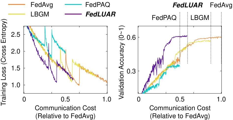
Figure 5: The learning curve comparisons for CIFAR-100 (Wide-ResNet28-10). The x-axis represents the communication cost relative to FedAvg. FedPAQ has the least amount of communication cost for 300 epochs, however it loses the accuracy too much. FedLUAR nearly does not drop the accuracy while significantly reducing the communication cost.

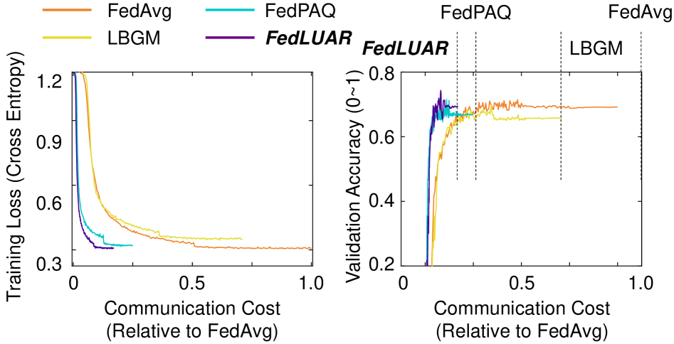
Figure 6: The learning curve comparisons for FEMNIST (CNN). The x-axis represents the communication cost relative to FedAvg. FedLUAR significantly reduces the communication cost while maintaining the model accuracy.

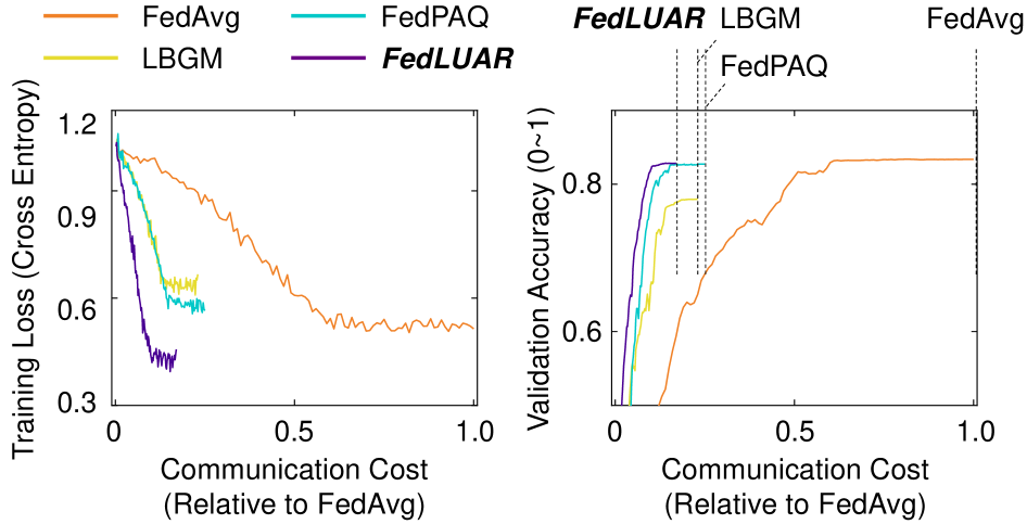
Figure 7: The learning curve comparisons for AG News (DistillBERT). The x-axis represents the communication cost relative to FedAvg. Likely to other behcnamrks, FedLUAR achieves the best accuracy faster than other SOTA methods.

References

- Alistarh et al. [2018] Dan Alistarh, Torsten Hoefler, Mikael Johansson, Sarit Khirirat, Nikola Konstantinov, and Cédric Renggli. The convergence of sparsified gradient methods. In Conference on neural information processing systems. NeurIPS, 2018.
- Azam et al. [2021] Sheikh Shams Azam, Seyyedali Hosseinalipour, Qiang Qiu, and Christopher Brinton. Recycling model updates in federated learning: Are gradient subspaces low-rank? In International Conference on Learning Representations. ICLR, 2021.
- Bibikar et al. [2021] Sameer Bibikar, Haris Vikalo, Zhangyang Wang, and Xiaohan Chen. Federated dynamic sparse training: Computing less, communicating less, yet learning better. In Proceedings of the AAAI Conference on Artificial Intelligence, 2021.
- Caldas et al. [2018] Sebastian Caldas, Sai Meher Karthik Duddu, Peter Wu, Tian Li, Jakub Konečnỳ, H Brendan McMahan, Virginia Smith, and Ameet Talwalkar. Leaf: A benchmark for federated settings. arXiv preprint arXiv:1812.01097, 2018.
- Chen and Vikalo [2024] Huancheng Chen and Haris Vikalo. Mixed-precision quantization for federated learning on resource-constrained heterogeneous devices. In Proceedings of the IEEE/CVF Conference on Computer Vision and Pattern Recognition, pages 6138–6148, 2024.
- Geeho Kim [2024] Bohyung Han Geeho Kim, Jinkyu Kim. Communication-efficient federated learning with accelerated client gradient. In Computer Vision and Pattern Recognition. CVPR, 2024.
- Gunesli et al. [2021] Gozde N Gunesli, Mohsin Bilal, Shan E Ahmed Raza, and Nasir M Rajpoot. Feddropoutavg: Generalizable federated learning for histopathology image classification. arXiv preprint arXiv:2111.13230, 2021.
- Haddadpour et al. [2021] Farzin Haddadpour, Mohammad Mahdi Kamani, Aryan Mokhtari, and Mehrdad Mahdavi. Federated learning with compression: Unified analysis and sharp guarantees. In International Conference on Artificial Intelligence and Statistics, pages 2350–2358. PMLR, 2021.
- He et al. [2016] Kaiming He, Xiangyu Zhang, Shaoqing Ren, and Jian Sun. Deep residual learning for image recognition. In Proceedings of the IEEE conference on computer vision and pattern recognition, pages 770–778, 2016.
- Hu et al. [2024] Ming Hu, Yue Cao, Anran Li, Zhiming Li, Chengwei Liu, Tianlin Li, Mingsong Chen, and Yang Liu. Fedmut: Generalized federated learning via stochastic mutation. In Proceedings of the AAAI Conference on Artificial Intelligence, 2024.
- Hyeon-Woo et al. [2021] Nam Hyeon-Woo, Moon Ye-Bin, and Tae-Hyun Oh. Fedpara: Low-rank hadamard product for communication-efficient federated learning. In International Conference on Learning Representations. ICLR, 2021.
- Jiang et al. [2022] Yuang Jiang, Shiqiang Wang, Victor Valls, Bong Jun Ko, Wei-Han Lee, Kin K Leung, and Leandros Tassiulas. Model pruning enables efficient federated learning on edge devices. IEEE Transactions on Neural Networks and Learning Systems, 34(12):10374–10386, 2022.
- Jiang et al. [2023] Zhida Jiang, Yang Xu, Hongli Xu, Zhiyuan Wang, Jianchun Liu, Qian Chen, and Chunming Qiao. Computation and communication efficient federated learning with adaptive model pruning. IEEE Transactions on Mobile Computing, 23(3):2003–2021, 2023.
- Keskar et al. [2017] Nitish Shirish Keskar, Dheevatsa Mudigere, Jorge Nocedal, Mikhail Smelyanskiy, and Ping Tak Peter Tang. On large-batch training for deep learning: Generalization gap and sharp minima. In International Conference on Learning Representations. ICLR, 2017.
- Konečnỳ et al. [2016] Jakub Konečnỳ, H Brendan McMahan, Felix X Yu, Peter Richtárik, Ananda Theertha Suresh, and Dave Bacon. Federated learning: Strategies for improving communication efficiency. arXiv preprint arXiv:1610.05492, 2016.
- Krizhevsky [2009] Alex Krizhevsky. Learning multiple layers of features from tiny images. Technical report, 2009.
- Lee et al. [2023a] Sunwoo Lee, Chaoyang He, and Salman Avestimehr. Achieving small-batch accuracy with large-batch scalability via hessian-aware learning rate adjustment. Neural Networks, 158:1–14, 2023a.
- Lee et al. [2023b] Sunwoo Lee, Tuo Zhang, and A Salman Avestimehr. Layer-wise adaptive model aggregation for scalable federated learning. In Proceedings of the AAAI Conference on Artificial Intelligence, volume 37, pages 8491–8499, 2023b.
- Li et al. [2024] Andy Li, Milan Markovic, Peter Edwards, and Georgios Leontidis. Model pruning enables localized and efficient federated learning for yield forecasting and data sharing. Expert Systems with Applications, 242:122847, 2024.
- Li et al. [2020] Tian Li, Anit Kumar Sahu, Manzil Zaheer, Maziar Sanjabi, Ameet Talwalkar, and Virginia Smith. Federated optimization in heterogeneous networks. In Annual Conferences on Machine Learning and System. MLSys, 2020.
- Lin et al. [2020] Tao Lin, Lingjing Kong, Sebastian Stich, and Martin Jaggi. Extrapolation for large-batch training in deep learning. In International Conference on Machine Learning, pages 6094–6104. PMLR, 2020.
- Mehmeti-Göpel and Wand [2024] Christian HX Mehmeti-Göpel and Michael Wand. On the weight dynamics of deep normalized networks. In International Conference on Machine Learning. ICML, 2024.
- Phan et al. [2020] Anh-Huy Phan, Konstantin Sobolev, Konstantin Sozykin, Dmitry Ermilov, Julia Gusak, Petr Tichavskỳ, Valeriy Glukhov, Ivan Oseledets, and Andrzej Cichocki. Stable low-rank tensor decomposition for compression of convolutional neural network. In European Conference on Computer Vision, pages 522–539. Springer, 2020.
- Qinbin Li [2021] Dawn Song Qinbin Li, Bingsheng He. Model-contrastive federated learning. In Computer Vision and Pattern Recognition. CVPR, 2021.
- Reddi et al. [2021] Sashank Reddi, Zachary Charles, Manzil Zaheer, Zachary Garrett, Keith Rush, Jakub Konečnỳ, Sanjiv Kumar, and H Brendan McMahan. Adaptive federated optimization. In International Conference on Learning Representations. ICLR, 2021.
- Reisizadeh et al. [2020] Amirhossein Reisizadeh, Aryan Mokhtari, Hamed Hassani, Ali Jadbabaie, and Ramtin Pedarsani. Fedpaq: A communication-efficient federated learning method with periodic averaging and quantization. In International conference on artificial intelligence and statistics, pages 2021–2031. PMLR, 2020.
- Sanh et al. [2019] Victor Sanh, L Debut, J Chaumond, and T Wolf. Distilbert, a distilled version of bert: Smaller, faster, cheaper and lighter. arxiv 2019. arXiv preprint arXiv:1910.01108, 2019.
- Vogels et al. [2020] Thijs Vogels, Sai Praneeth Karimireddy, and Martin Jaggi. Practical low-rank communication compression in decentralized deep learning. In Conference on neural information processing systems. NeurIPS, 2020.
- Wen et al. [2017] Wei Wen, Cong Xu, Feng Yan, Chunpeng Wu, Yandan Wang, Yiran Chen, and Hai Li. Terngrad: Ternary gradients to reduce communication in distributed deep learning. Advances in neural information processing systems, 30, 2017.
- Wu et al. [2022] Chuhan Wu, Fangzhao Wu, Lingjuan Lyu, Yongfeng Huang, and Xing Xie. Communication-efficient federated learning via knowledge distillation. Nature communications, 13(1):2032, 2022.
- Yang et al. [2021] Haibo Yang, Minghong Fang, and Jia Liu. Achieving linear speedup with partial worker participation in non-iid federated learning. In International Conference on Learning Representations. ICLR, 2021.
- You et al. [2017] Yang You, Igor Gitman, and Boris Ginsburg. Large batch training of convolutional networks. arXiv preprint arXiv:1708.03888, 2017.
- Zagoruyko and Komodakis [2016] Sergey Zagoruyko and Nikos Komodakis. Wide residual networks. arXiv preprint arXiv:1605.07146, 2016.
- Zhang et al. [2015] Xiang Zhang, Junbo Zhao, and Yann LeCun. Character-level convolutional networks for text classification. Advances in neural information processing systems, 28, 2015.