Strong Lensing Effect and Quasinormal Modes of Oscillations of Black Holes in $\boldsymbol{f(R,T)}$ Gravity Theory

Abstract

In this work, we analyze the strong lensing phenomenon and quasinormal modes (QNMs) in the case of black holes (BHs) surrounded by fluids within the framework of $f(R,T)$ gravity, adopting a minimally coupled model of the theory. Our analysis is conducted for three surrounding fields corresponding to three different values of the parameter $\omega$ of the equations of state, each representing a unique class of BH solutions. A universal method developed by V. Bozza is employed for strong lensing analysis and the WKB approximation method to compute the QNMs of oscillation of the BHs. The influence of the model parameter $\beta$ on the deflection angle and associated lensing coefficients is analyzed. Our findings on lensing reveal that smaller values of $\beta$ cause photon divergence at larger impact parameters, with the results converging to the Schwarzschild limit as $\beta\to-16.7551$ for (for $\omega=0)$, $\beta\to-18.8495$ (for $\omega=1/3)$ and $\beta\to-13.7088$ (for $\omega=-2/3)$. Extending the analysis to the supermassive BH SgrA*, we examine the outermost Einstein rings, estimate three lensing observables: angular position $\vartheta_{\infty}$, angular separation $s$ and relative magnification $r_{\text{mag}}$ for the BHs. For a specific value of $\beta$, BHs with different field configurations exhibit substantial variations in their observable properties. The variation of amplitude and damping of QNMs with respect to the model parameter $\beta$ is analyzed for the BHs. We found that the $\beta$ parameter has a direct correlation with the amplitude and an inverse relation with the damping of the QNMs. Further, we use the time domain analysis to verify the results and found a good match between the two methods.

I Introduction

Black holes (BHs) have gained significant attention in recent times. The two major milestones of modern physics that have propelled the growing interest in the field of BH physics are the discovery of gravitational waves (GWs) by the LIGO and Virgo team in 2015 [1, 2, 3, 4, 5, 6], and the first ever image of the BH M87^∗ at the center of M87 galaxy, by the Event Horizon Telescope (EHT) group in 2019 [7, 8, 9, 10, 11, 12]. Since then a lot of efforts have been directed towards a better understanding of the physics of BHs. Though a lot remains to be uncovered about BHs, some insights have been achieved and it is expected that advanced detectors of the future will shed more light regarding these mysterious objects. BHs came out as a mathematical solution of Einstein field equations in the General Relativity (GR) framework in 1916, obtained by Karl Schwarzschild for the vacuum case. Ever since a number of papers have derived BH solutions in different spacetimes and different gravity theories (see Ref. [13, 14, 15] for a review).

GR is the most fundamental and robust theory of gravity thus far. GR has been backed by two most fascinating and crucial observations of recent times in addition to earlier supporting observations [16]. One is the detection of GWs and the other is the snap of the direct image of the BH at the center of galaxy M87 [17] as mentioned already. However, there are some issues with GR that need to be addressed so that a complete theory of gravity can be obtained. GR faces the normalization issue in the high energy regime [18]. GR can not explain the dark components in the Universe, especially it fails in the IR regime as it cannot explain the accelerated expansion of the Universe as recently confirmed [19, 20] and can not predict anything regarding the existence of dark matter [21]. It has compatibility issues with quantum mechanical phenomena [22]. These issues have motivated researchers to look for modified as well as alternative theories of gravity (ATGs) [17, 23, 24, 25]. Physicists modify either the matter-energy sector or the geometry part of the Eistein field equations in their efforts to mitigate the issues faced by GR. The former way of modification leads to the theories of dark energy and latter one leads to the development of modified theories of gravity (MTGs). Some of the most pursued MTGs are $f(R)$ gravity [26, 27, 28], $f(R,T$) gravity [29, 30], Rastall gravity [33, 34], $f(R,L_{m}$) gravity [35] and so on. On the other hand ATGs are based on fundamentally different geometrical approaches than the approach of GR. One of the most studied ATGs is the $f(Q)$ gravity [31, 32] theory.

Gravitational lensing is a gravitational effect on light, which occurs due to the bending of light when passing the curved spacetime produced by massive objects such as galaxies, galaxy clusters, BHs, etc. It was predicted by Einstein in 1915 in his theory of GR [36] and now become an indispensable tool in modern astrophysics and cosmology [37, 38, 39, 40]. This phenomenon was first observed around the sun by Eddington, Dyson and Davidson during the time of the solar eclipse in 1919, when starlight from the Hyades cluster passed near the sun. It was recorded as the first experimental verification of GR [41]. The lensing effect produces magnified, distorted images and delays the time taken by light to arrive at the observer. Specifically, lensing in the strong field limit exhibits distinct and notable features, and the deflection angle offers a critical pathway for exploring the optical characteristics of lensing objects. Consequently, as a lensing object, BHs serve as unique platforms for studying the effects of strong gravitational fields. Within this limit, a ray of light passing very close to the objects becomes highly nonlinear. The trajectories followed by light in such propagation undergo multiple circular loops around the object before leaving it [43, 42]. As a result, a series of discrete images, referred to as relativistic images are formed from a single object which cannot be explained by classical weak-field lensing theories [44, 45]. Indeed, gravitational lensing functions as a reliable astrophysical technique for investigating the gravitational fields of massive objects and shedding light on the elusive nature of dark matter [46, 47, 48].

In the strong field regime, Darwin’s pioneering work on the interpretation of Einstein’s equations for orbits around the sun to determine whether particles or light rays captured by the sun is served as the groundwork for subsequent developments in this area [45]. Over the years, investigations in the strong field limit have gained significant attention due to their potential to extract information about BHs [43, 49, 50, 51, 52, 53, 55, 54, 56, 57, 59, 58, 60]. A wide range of work has been performed on the strong deflection lensing extensively for Schwarzschild BHs [61, 62, 64, 63, 65]. Virbhadra and his co-workers have made a significant contribution to the study of gravitational lensing by introducing the lens equation in the investigations of the strong field regime [65, 64]. Later they analyzed the formation and properties of relativistic images for a Schwarzschild BH in this context [66, 67]. Further investigations expanding to other static and symmetric BH spacetimes have been performed by many researchers [68, 69, 50, 70, 71, 51, 72, 85]. In fact, the past decade has witnessed a significant progress in studies on gravitational lensing including investigations for naked singularities [74, 75, 76], wormholes [77, 78, 79, 80], and other exotic entities [81, 82]. A plethora of parallel efforts have been made on strong field deflection in GR as well as in context of MTGs, revealing remarkable phenomena such as relativistic images and shadow formation [84, 85, 83, 86, 87, 88, 96, 89, 90, 91, 93, 94, 95, 92, 97]. However, when one considers the MTGs, the deflection angle encapsulates additional information about deviations from the Schwarzschild or Kerr metrics. By analyzing the deflection in such scenarios, one can constrain the parameters of MTGs and assess their viability in describing astrophysical observations.

Detection of GWs has opened up a new window to look at the Universe and develop our understanding on how gravity works in strong gravity regimes. When a BH is perturbed by some field, it oscillates and releases the excess energy to go back to its steady state. This release of energy is in the form of spacetime ripples with very minute amplitudes and decaying as it travels through spacetime. These are nothing but quasinormal modes (QNMs) of oscillations [98, 99]. QNMs have not been detected yet but it is believed that future detectors of GWs will be able to observe them. The concept of QNMs theoretically emerged for the first time via the work of Vishveshwara in 1970 [100]. Later, in 1975, Chandrasekhar and Detweiler computed the QNMs for the first time [101]. Schrutz and Will computed the QNMs for the first time using the WKB approximation method [102]. Since then many numerical as well as analytical methods have been employed to compute the QNMs. Konoplya developed the WKB method up to the 13th order along with the Padé averaging technique [103]. Other methods such as the asymptotic iteration method (AIM), Bernstein spectral method, Leaver’s technique, etc. have been widely used in the literature to compute the QNMs (see Ref. [98] for a review). In Ref. [104], the authors computed QNMs of BHs in scalar-vector-tensor (SVT) gravity with a surrounding quintessence field. They also studied the thermodynamic and optical properties of the obtained BH solution. Ref. [105] discusses BHs in MTGs in both static and rotating configurations and studies their optical properties. Recently, the authors in Ref. [106] computed a class of Kiselev BH solutions in the framework of $f(R,T)$ gravity. In another work [107], the authors obtained different solutions of BHs considering various models of the $f(R,T)$ gravity framework and studied their properties. QNMs of BH solutions in the framework of the Hu-Sawicki model of $f(R)$ gravity have been studied in Ref. [17].

Motivated by the factors mentioned above, our study aims to explore the strong limit lensing characteristics and QNMs of BHs within the framework of the $f(R,T)$ gravity. The recent formulation of a BH spacetime in this theoretical framework [106, 107] has sparked our interest in exploring gravitational bending effects as well as QNMs of the BH. In the strong field lensing investigation, the technique proposed by V. Bozza [43] is adopted, whereas for QNMs calculations the WKB approximation is employed.

The rest of the paper is structured as follows: In Section II, we outline the theoretical framework of the study. In Section III, we focus on the derivation of the gravitational bending angle in the strong field limit in the BH spacetime. Additionally, this section includes the computation and analysis of lensing observables by considering the supermassive BH SgrA* as a $f(R,T)$ gravity BH. Then we compute QNMs of the BH in Section IV. Section V presents the time profile analysis of the BH. Finally, we present our concluding remark in Section VI.

II $\boldsymbol{f(R,T)}$ Gravity Black Holes

The $f(R,T)$ gravity is a modification of Einstein’s GR where the gravitational Lagrangian $\mathcal{L}$ in the Einstein-Hilbert action is generalized as a function of the Ricci scalar $R$ and the trace $T$ of the energy-momentum tensor $T_{\mu\nu}$. The core concept of this theory is the coupling between the geometry and matter. This can significantly influence the BH’s spacetime by introducing an extra term in the field equations. Thus the action in this theory is given as [108]

$$S=\frac{1}{2\kappa^{2}}\int\!\sqrt{-\,g}\,{f(R,T)}\,d^{4}x+\int\!\sqrt{-\,g}\,\mathcal{L}_{m}\,d^{4}x,$$ (1)

where $\mathcal{L}_{m}$ is the Lagrangian density of matter field, $g$ is determinant of the metric $g_{\mu\nu}$ and $\kappa^{2}=8\pi G=1/M^{2}_{pl}$. $G$ and $M_{pl}$ are the gravitational constant and reduced Planck mass respectively. The energy-momentum tensor of the matter field can be written as

$$T_{\mu\nu}=-\,\frac{2\,\delta(\sqrt{-\,g}\mathcal{L}_{m})}{\sqrt{-\,g}\ \delta g^{\mu\nu}}=-\,2\ \frac{\partial\mathcal{L}_{m}}{\partial g^{\mu\nu}}+g_{\mu\nu}\,\mathcal{L}_{m}.$$ (2)

This equation gives us the trace of $T_{\mu\nu}$ as

$$T=-\,2\,g^{\mu\nu}\frac{\partial\mathcal{L}_{m}}{\partial g^{\mu\nu}}+4\,\mathcal{L}_{m}.$$ (3)

The variation of the action (1) with respect to the metric $g_{\mu\nu}$ yields the field equations of this gravity theory as

$$F_{R}\,R_{\mu\nu}-\frac{1}{2}\,f(R,T)\,g_{\mu\nu}+\left(g_{\mu\nu}\square-\nabla_{\mu}\nabla_{\nu}\right)F_{R}=\kappa^{2}T_{\mu\nu}-F_{T}\left(T_{\mu\nu}+\theta_{\mu\nu}\right),$$ (4)

where $F_{R}=df(R,T)/dR$, $F_{T}=df(R,T)/dT$ and the energy tensor $\theta_{\mu\nu}$ defined as [108, 109]

$$\theta_{\mu\nu}=g^{ab}\,\frac{\delta{T}_{ab}}{\delta{g^{\mu\nu}}}=-\,2\,T_{\mu\nu}+g_{\mu\nu}\,\mathcal{L}_{m}-2\,g^{ab}\frac{\partial^{2}{\mathcal{L}_{m}}}{\partial{g^{\mu\nu}}\partial{g^{ab}}}.$$ (5)

It is noteworthy that depending on the different forms of the function $f(R,T)$, the models of this gravity may be placed into three categories, viz., the minimally, non-minimally and purely non-minimally coupling models. The forms of these three types are proposed respectively as [110, 111]: $f(R,T)=f_{1}(R)+f_{2}(T)$, $f(R,T)=f_{1}(R)[1+f_{2}(T)]$ and $f(R,T)=f_{1}(R)\,f_{2}(T)$. In our work, we assume the minimally coupled matter and geometry sector in $f(R,T)$ gravity and so we consider the first kind of model for the analysis of the BHs spacetime in this theory. However, investigations of BHs characteristics in such models of $f(R,T)$ modified gravity result in some remarkable features that are attributed to these compact objects surrounded by some fluids [112, 106]. Recently, as mentioned earlier a study by Ref. [107] has derived the BH solutions in the context of this gravity theory and explored the thermodynamic properties of these BHs from their thermodynamic topology and thermodynamic geometry. Following this reference, we consider a static spherically symmetric metric ansatz in the form:

$$ds^{2}=A(r)dt^{2}-B(r)dr^{2}-r^{2}(d\theta^{2}+\sin^{2}\!\theta\,d\phi^{2}).$$ (6)

As mentioned above, we are focusing on a minimally coupled $f(R,T)$ model characterized by the parameters $\alpha$ and $\beta$, expressed in the following form:

$$f(R,T)=\alpha f_{1}(R)+\beta f_{2}(T),$$ (7)

where $f_{1}(R)=R$ and $f_{2}(T)=T$ are considered. In this study, the trace of the energy-momentum tensor $T$ is connected to the spherically symmetric Kiselev BHs. The energy-momentum tensor governing Kiselev BHs is effectively associated with an anisotropic fluid, whose components satisfy the following relations [112, 106]:

$$T^{t}_{t} =T^{r}_{r}=\rho,$$ (8)

$$T^{\theta}_{\theta} =T^{\phi}_{\phi}=-\,\frac{1}{2}\rho\,(3\,\omega+1),$$ (9)

where $\rho$ represents the energy density of the fluid and $\omega$ is the equation of state parameter. Choosing the matter Lagrangian density $L_{m}=P=-\,(p_{r}+2\,p_{t})/3$, with the radial and tangential pressures $p_{r}=-\,\rho$ and $p_{t}=(3\,\omega+1)/2$ respectively, calculated from the general form of the energy-momentum tensor $T_{\mu\nu}=-\,p_{t}g_{\mu\nu}+(\rho+p_{t})u_{\mu}u_{\nu}+(p_{r}-p_{t})v_{\mu}v_{\nu}$ of an anisotropic fluid, where $u_{\mu}$ and $v_{\mu}$ represent the radial four-vectors and the four-velocity vectors respectively [113], equation (5) can be rewritten as

$$\theta_{\mu\nu}=-\,2T_{\mu\nu}-\frac{1}{3}(p_{r}+2p_{t})g_{\mu\nu}.$$ (10)

Using these results the solution is obtained for the metric function (6) of spacetime in the $f(R,T)$ gravity framework with the model (7) as follows [107]:

$$A(r)=\frac{1}{B(r)}=1-\frac{2M}{r}+c_{2}\,r^{-\frac{8(\beta\omega+\pi(6\omega+2))}{16\pi-\beta(\omega-3)}},$$ (11)

where $M$ represents the total mass of the BH enclosed by the surrounding fluid and $c_{2}$ is a constant which will be taken as unity throughout the study [112, 107]. It is evident from equation (11) that this BH solution is independent of the parameter $\alpha$. Notably, in our analysis, we are concerned with three choices of the parameter $\omega$ corresponding to dust field ($\omega=0$), radiation field ($\omega=1/3$) and quintessence field ($\omega=-2/3$) around the BH which yield three different BH solutions. In the absence of fluid, the solution (11) simplifies to the Schwarzschild BH solution, but simply $\omega\to 0$, $\omega\to 1/3$ or $\omega\to-2/3$ do not reduce the solution to a BH surrounded by dust, radiation or a quintessence field in the framework of GR due to the presence of parameter $\beta$. When $\beta\to 0$, $\omega\to 0$, the solution corresponds to the metric of a Schwarzschild BH with an effective mass $M_{eff}=2M-c_{2}$ [106]. Similarly, for $\beta\to 0$, $\omega\to 1/3$, the solution behaves as the Reissner-Nordström BH with effective charge $q^{2}_{eff}=c_{2}$ [106, 107].

     

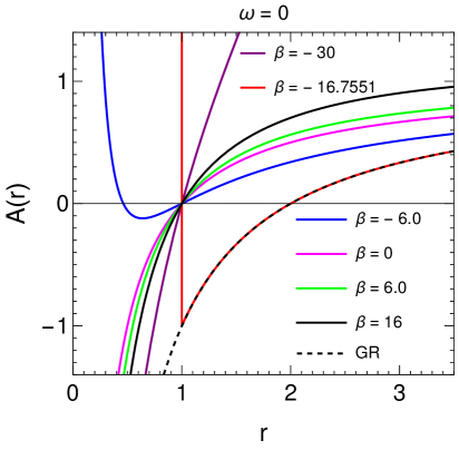
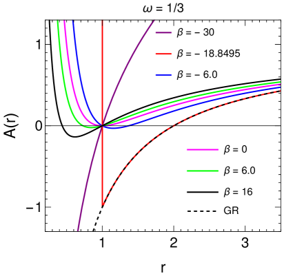
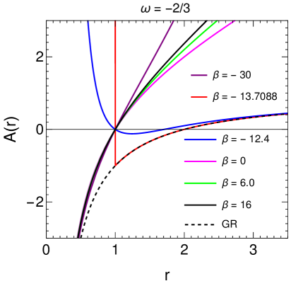
Figure 1: The horizon structure of minimally coupled $f(R,T)$ gravity BHs with different values of $\omega$ as well as for different values of model parameter $\beta$.

It also needs to outline some other key aspects of the considered BHs’ solution to ensure the completeness of the subsequent analyses. As a part, we plot the variation of the function $A(r)$ with respect to radial distance $r$ as shown in Fig. 1 to analyze the horizon structures of the BHs under consideration. It is done by the root analysis of equation $A(r)=0$ for different values of model parameter $\beta$ as the positive roots of the equation $A(r)=0$ correspond to the locations of horizons of the BHs. It is observed that our BHs’ solution (11) exhibits a fixed horizon at $r=1$ irrespective of values $\beta\geq 0$ or $\beta<0$. This fixed horizon remains unaffected by $\omega$ as well. Of course, it is not seen as the event horizon for the whole domain of parameter $\beta$ in all the classes of BHs. In the first representation with $\omega=0$, for $\beta\geq 0$, it is the event and the only horizon of the considered BH. In contrast to this, one may find mostly two distinct horizons for $\beta<0$ along with the horizon at $r=1$. For example, for small negative values of the parameter $\beta$ the first (Cauchy) horizon appears at $r<1$, whereas for large negative values of $\beta$ the second (event) horizon shifts to $r>1$. However, at sufficiently large negative values of $\beta$, the BH again admits only a single horizon at $r=1$. In the second plot of the figure where $\omega=1/3$, it is observed that the BH admits two horizons with one fixed event horizon at $r=1$ and the Cauchy horizon at $r<1$ for $\beta>0$, whereas $\beta<0$ pushes the event horizon to $r>1$ region by making a transition of $r=1$ as the Cauchy horizon. In addition, there exists only a single horizon at the common point $r=1$ for $\beta=0$ in this situation also. Moreover, similar to the first consideration, the BH has a single horizon for significantly large negative values of $\beta$. On the other hand, BH with the quintessence field as a surrounding possesses an event horizon in the region $r>1$ for smaller negative values of $\beta$ with Cauchy horizon at $r=1$. Otherwise it shows a single horizon at the fixed position as mentioned. Interestingly, with the Cauchy horizon at $r=1$, the event horizons of our BHs coincide with the Schwarzschild BH horizon at $r=2$ for $\beta=-16.7551$, $\beta=-18.8495$ and $\beta=-13.7088$ in the first ($\omega=0$), second ($\omega=1/3$) and third ($\omega=-2/3$) situations respectively. Moreover, it is examined numerically that the modified BHs under consideration exhibit non-asymptotically flat behavior for $\beta<-16.7551$ in the $\omega=0$ case, $\beta<-18.8495$ when $\omega=1/3$ and $\beta<-13.7088$ in the $\omega=-2/3$ scenario. Recognizing the importance of these critical values of $\beta$ on the geometry of the spacetime of the $f(R,T)$ BHs, we limit our analysis to $\beta\geq-16.7551$, $\beta\geq-18.8495$ and $\beta\geq-13.7088$ for the respective cases. It can be inferred that despite the event horizons at the same location, the spacetime geometry of the considered BHs differs fundamentally from that of the Schwarzschild BH due to the presence of the Cauchy horizon. Thus observing such a horizon structure scenario, we can remark that the structure of a minimally coupled $f(R,T)$ gravity BHs changes typically and reflects a significant change in the spacetime’s causal structure as the parameter $\beta$ varies.

III Bending of Light in the Strong Field Limit

In this section, we explore the bending of light in the strong field limit of the $f(R,T)$ gravity BHs spacetime. In the limit of strong gravitational lensing, a photon coming from a far distant source passes extremely close to a massive object and encounters its intense gravitational field. As a result, it is deviated at a closest approach distance $r=r_{0}$ before moving to the observer at infinity. The path of the photon undergoes sharp bending as it approaches closer to the object leading to an increased deflection angle. At a certain value of $r_{0}$ the deflection angle becomes $2\pi$ causing the photon to make a complete loop around the BH. A further reduction of $r_{0}$, the photon orbits the BH multiple times, thereby resulting in the deflection angle greater than $2\pi$. When $r_{0}$ becomes equal to the radius of the photon sphere $r_{p}$, the deflection angle diverges [114, 43, 115, 69, 116]. Here our objective is to analyze the deflection angle and related lensing observables in the strong field limit for a static, spherically symmetric BH spacetime described by the line element (6). For this, we assume photon trajectories confined in the equatorial plane $(\theta=\pi/2)$ of the object and adopt the strong lensing effect investigation method developed by V. Bozza, suitable for the motion of photons described by a standard geodesic equation in any spacetime and within any gravitational framework [43]. Notably, the entire trajectory of the photon is governed by the equation, $g_{\mu\nu}k^{\mu}k^{\nu}=0,$ where $k^{\mu}=dx^{\mu}/d\tau$ represents the wave number of the photon and $\tau$ is the affine parameter along its trajectory [115, 117]. Thus, considering $C(r)=r^{2}$ in equation (6), the equation of photon trajectories can be written as [118, 119]

$$A(r)\,\dot{t}^{2}-B(r)\,\dot{r}^{2}-C(r)\,\dot{\phi}^{2}=0.$$ (12)

As the spherical symmetry of the metric (6) ensures the conservation of energy $E=A(r)\dot{t}$ and angular momentum $L=r^{2}\dot{\phi}$ respectively during the journey, hence specified by these two constant quantities and defining impact parameter $\zeta$ as $\zeta=L/E$, the above equation of trajectories (12) can be rewritten as [118, 115]

$$\dot{r}^{2}=V_{eff}(r),$$ (13)

where $V_{eff}(r)$ is the effective radial potential for the motion of a photon and is defined as

$$V_{eff}(r)=E^{2}\left[1-\zeta^{2}\frac{A(r)}{r^{2}}\right].$$ (14)

     

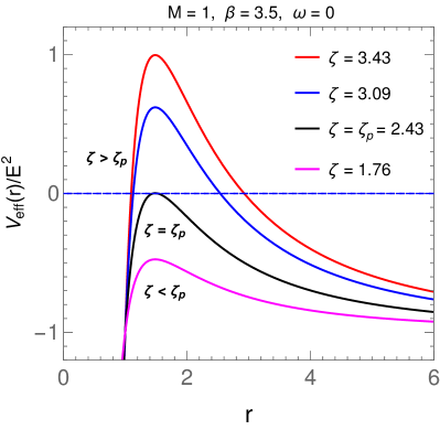
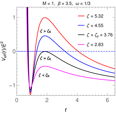
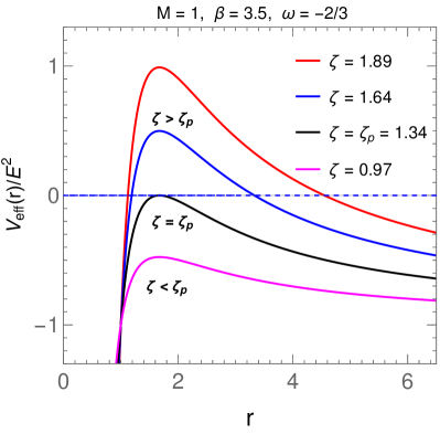
Figure 2: Variation of the effective potential $V_{eff}(r)$ for different values of $\omega$ as a function of radial coordinate $r$ for different values of impact parameter $\zeta$.

The above equation characterizes various possible photon orbits, which are graphically represented in Fig. 2 for $\omega=0,$ $1/3$ and $-2/3$. The figure depicts the effective radial potential corresponding to different impact parameter values such as $\zeta<\zeta_{p}$,  $\zeta=\zeta_{p}$ and $\zeta>\zeta_{p}$, which describe three different orbits of a photon. Here, $\zeta_{p}$ is the critical or minimum impact parameter defined at the photon sphere radius $r_{p}$ [117, 116]. A photon with impact parameter $\zeta<\zeta_{p}$ is captured by the strong field of the BHs, while one with $\zeta>\zeta_{p}$, is deflected by the BHs when reaches $r=r_{0}$ and with $\zeta=\zeta_{p}$, whirls the BHs for sometimes at photon sphere radius $r_{p}$ before leaving it [120]. The photon sphere radius is the largest positive root of the equation [121, 43, 65],

$$\frac{C^{\prime}(r)}{A^{\prime}(r)}=\frac{C(r)}{A(r)}.$$ (15)

For our BHs’ solution (11) this equation takes the form:

$$\frac{3M}{r}-\frac{4(\beta\omega+\pi(6\omega+2))r^{-\frac{8(\beta\omega+\pi(6\omega+2))}{16\pi-\beta(\omega-3)}}}{16\pi-\beta(\omega-3)}-r^{-\frac{8(\beta\omega+\pi(6\omega+2))}{16\pi-\beta(\omega-3)}}-1=0.$$ (16)

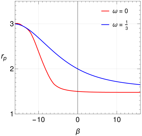
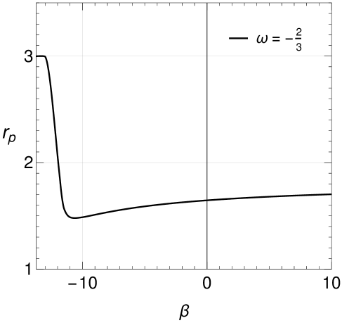
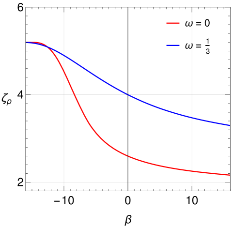
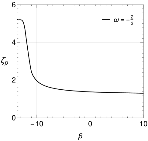
Figure 3: Behaviors of photon sphere radius $r_{p}$ and critical impact parameter $\zeta_{p}$ for minimally coupled $f(R,T)$ gravity BHs as a function of model parameter $\beta$ for $\omega=0,$ $1/3$ and $-2/3$ respectively.

Due to the complexity of this equation the photon sphere radius $r_{p}$ for different classes of BHs are computed numerically for a range of $\beta$ values and a graphical representation of their dependence on the parameter $\beta$ is shown in Fig. 3. Furthermore, at the point of closest approach $r=r_{0}$ the impact parameter $\zeta_{0}$ can be expressed from the orbit equation (13) as $\zeta_{0}=\sqrt{C(r_{0})/A(r_{0})}$. This expression allows us to determine the critical impact parameter at $r_{0}=r_{p}$ as given below:

$$\zeta_{p}=\sqrt{\frac{C(r_{p})}{A(r_{p})}}=\frac{r_{p}}{\sqrt{1-\frac{2M}{r_{p}}+\,r_{p}^{-\frac{8(\beta\omega+\pi(6\omega+2))}{16\pi-\beta(\omega-3)}}}}.$$ (17)

We depict its behavior as a function of $\beta$ in Fig. 3 along with the same for $r_{p}$ for all three cases. The figure demonstrates that both $r_{p}$ and $\zeta_{p}$ for $\omega=-2/3$ show steep initial fall in comparison to $\omega=0$ and $1/3$ cases.

III.1 Deflection angle in minimally coupled $f(R,T)$ gravity spacetime

The deflection angle $\hat{\alpha}$ which is formed between the asymptotic paths of the incoming and outgoing photons can be expressed using orbit equation (13) as [123, 122, 43]

$$\hat{\alpha}(r_{0})=I(r_{0})-\pi,$$ (18)

where

$$I(r_{0})=2\!\int_{r_{0}}^{\infty}\!\frac{1}{\sqrt{A(r)C(r)}\sqrt{\frac{C(r)A(r_{0})}{C(r_{0})A(r)}-1}}\,dr.$$ (19)

As mentioned earlier, we focus on the investigation of the deflection angle in the strong field limit where photon trajectories approach closely to the photon sphere of the lensing BHs. For completeness of our analysis following the Bozza’s method we define a new variable $z$ as [115, 42, 51]

$$z=1-\frac{r_{0}}{r},$$ (20)

and rewrite the integral (19) as [43, 51]

$$I(r_{0})=\int_{0}^{1}\!N(z,r_{0})\,g(z,r_{0})\,dz,$$ (21)

where the functions $N(z,r_{0})$ and $g(z,r_{0})$ can be written as follows [124, 51, 42]:

$$N(z,r_{0})=\frac{2r^{2}\sqrt{A(r)B(r)C(r_{0})}}{r_{0}\,C(r)},$$ (22)

and

$$g(z,r_{0})=\frac{1}{\sqrt{A(r_{0})-\frac{A(r)}{C(r)}\,C(r_{0})}}.$$ (23)

For any value of $z$ and $r_{0}$ the function $N(z,r_{0})$ is regular, whereas $g(z,r_{0})$ diverges as the photon approaches the photon sphere, i.e. when $z\to 0$. Therefore, the integral (21) can be decomposed into two parts, the regular part $I_{R}(r_{0})$ and the divergence part $I_{D}(r_{0})$ as given below [43]:

$$I(r_{0})=I_{D}(r_{0})+I_{R}(r_{0}),$$ (24)

where

$$I_{D}(r_{0})=\int_{0}^{1}\!N(0,r_{p})\,g_{0}(z,r_{0})\,dz,$$ (25)

$$I_{R}(r_{0})=\int_{0}^{1}\!\big{[}N(z,r_{0})\,g(z,r_{0})-N(0,r_{p})\,g_{0}(z,r_{0})\big{]}\,dz.$$ (26)

Next, to approximate the rate of divergence, the argument of the square root of $g(z,r_{0})$ is expanded to second-order in $z$ which results [43, 53]:

$$g(z,r_{0})\sim g_{0}(z,r_{0})=\frac{1}{\sqrt{m(r_{0})\,z+n(r_{0})\,z^{2}}},$$ (27)

where the coefficients $m(r_{0})$ and $n(r_{0})$ are obtained as [71, 125]

$$m(r_{0}) =\frac{r_{0}}{C(r_{0})}\left[A(r_{0})\,C^{\prime}(r_{0})-A^{\prime}(r_{0})\,C(r_{0})\right]$$

$$=2-\frac{6M}{r_{0}}+\left[1+\frac{4(\beta\omega+\pi(6\omega+2))}{(16\pi-\beta(\omega-3))}\right]2\,r_{0}^{\!-\frac{8(\beta\omega+\pi(6\,\omega+2))}{16\pi-\beta(\omega-3)}},$$ (28)

$$n(r_{0}) =\frac{r_{0}}{2\,C^{2}(r_{0})}\left[2\Big{(}C(r_{0})-r_{0}\,C^{\prime}(r_{0})\Big{)}\Big{(}A(r_{0})\,C^{\prime}(r_{0})-A^{\prime}(r_{0})\,C(r_{0})\Big{)}+r_{0}C(r_{0})\Big{(}A(r_{0})\,C^{\prime\prime}(r_{0})-A^{\prime\prime}(r_{0})C(r_{0})\Big{)}\right]$$

$$=\frac{6M}{r_{0}}-\left[1+\frac{8(\beta\omega+\pi(6\omega+2))}{16\pi-\beta(\omega-3)}+\frac{4(\beta\omega+\pi(6\omega+2))\left(\frac{8(\beta\omega+\pi(6\omega+2))}{16\pi-\beta(\omega-3)}+1\right)}{16\pi-\beta(\omega-3)}\right]r_{0}^{-\frac{8(\beta\omega+\pi(6\omega+2))}{16\pi-\beta(\omega-3)}}-1.$$ (29)

Eventually, when $r_{0}$ coincides with the radius of the photon sphere $r_{p}$, the coefficient $m(r_{0})$ becomes zero, thereby leaving $z^{-1}$ as the leading divergence term in the function $g_{0}(z,r_{0})$. It results in the logarithmic divergence of the integral (21). Accordingly, in the strong field limit an expression of the deflection angle in terms of impact parameter $\zeta$ can be approximated as [43, 126]

$$\hat{\alpha}(\zeta)=-\,\bar{a}\log\left(\frac{\zeta}{\zeta_{p}}-1\right)+\bar{b}+\mathcal{O}(\zeta-\zeta_{p}),$$ (30)

where $\bar{a}$, $\bar{b}$ represent the strong field limit lensing coefficients which are dependent on spacetime geometry. These coefficients are evaluated at $r_{0}=r_{p}$ and can be given by the following expressions [43, 125, 51]

$$\bar{a} =\frac{N(0,r_{p})}{2\sqrt{n(r_{p})}},$$ (31)

$$\bar{b} =-\,\pi+b_{R}+b_{D},$$ (32)

where $b_{D}$ and $b_{R}$ are defined as [51, 124]

$$b_{D} =\bar{a}\,\log\Bigg{[}\frac{r_{p}^{2}[C^{\prime\prime}(r_{p})\,A(r_{p})-C(r_{p})\,A^{\prime\prime}(r_{p})]}{\zeta_{p}\,\sqrt{A^{3}(r_{p})\,C(r_{p})}}\Bigg{]}$$

$$=\bar{a}\,\log\Bigg{[}2+\frac{[4M\,(16\pi-\beta(\omega-3))-8(\beta\omega+\pi(6\omega+2))\left(\frac{8(\beta\omega+\pi(6\omega+2))}{16\pi-\beta(\omega-3)}+1\right)r_{p}^{-\frac{8(\beta\omega+\pi(6\omega+2))}{16\pi-\beta(\omega-3)}+1}]}{(-\frac{2M}{r_{p}}+r_{p}^{-\frac{8(\beta\omega+\pi(6\omega+2))}{16\pi-\beta(\omega-3)}}+1)(16\pi-\beta(\omega-3))r_{p}}\Bigg{]},$$ (33)

$$b_{R} =I_{R}(r_{p})=\int_{0}^{1}\!\big{[}N(z,r_{p})\,g(z,r_{p})-N(0,r_{p})\,g_{0}(z,r_{p})\big{]}\,dz.$$ (34)

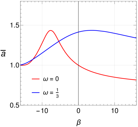
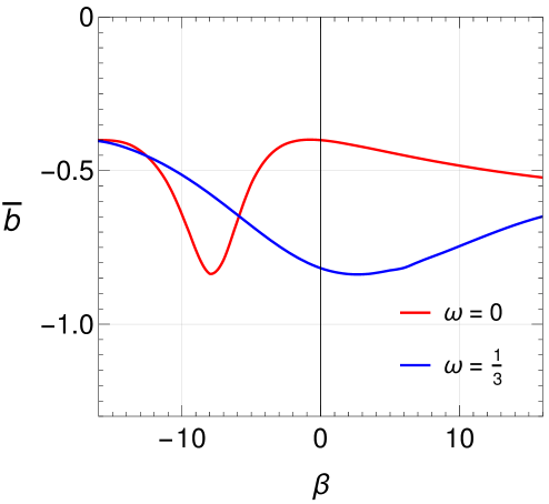
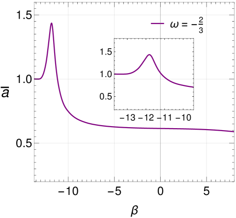
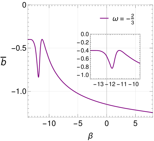
Figure 4: Behaviors of lensing coefficients $\bar{a}$ (left) and $\bar{b}$ (right) in minimally coupled $f(R,T)$ gravity BHs spacetime as a function of model parameter $\beta$ for $\omega=0$, $1/3$ and $-2/3$ cases.

To examine the behavior of the lensing coefficients in our modified BHs spacetime, we analyze their variation with model parameter $\beta$ in Fig. 4 and list their values in Tables 1, 2 and 3. For the $\omega=0$ case, the coefficient $\bar{a}$ initially increases moderately, reaches a peak around $\beta\approx-7$, then decreases as $\beta$ grows. When $\omega=1/3$, $\bar{a}$ exhibits a continuous but slow growth up to $\beta\approx 3.5$ then decreases smoothly as $\beta$ increases. In contrast, the coefficient $\bar{b}$ shows opposite trends. For the $\omega=0$ case, $\bar{b}$ decreases initially, reaches a minimum near $\beta\approx-7$, then increases as $\beta$ approaches to $0$. After that it follows a smooth declination for $\beta>0$, while for the $\omega=1/3$ case, $\bar{b}$ falls gradually up to $\beta\approx 3.5$ from the negative end and shows a slow growth beyond this value. On the other hand, for the $\omega=-2/3$ case, we observe significant variations in the lensing coefficients within the range of $-13.7088\leq\beta\leq-9.4381$. Similar to the cases of $\omega=0$ and $\omega=1/3$, coefficients $\bar{a}$ and $\bar{b}$ exhibit analogous behavior in this case also. However, for $\beta>-9.4381$, $\bar{a}$ goes almost as flat and $\bar{b}$ declines more rapidly than in the previous two cases. In fact, we observe contrasting behaviors of the lensing coefficients as a function of $\beta$ across these scenarios.

Table 1: Estimation of numerical values of lensing coefficients and corresponding impact parameter $\zeta_{p}$ for the $f(R,T)$ BHs with $\omega=0$ case. The impact parameter is listed as $\zeta_{p}/R_{s}$, where $R_{s}$ is the Schwarzschild radius. Here and in the following tables SBH represents the Schwarzschild BH.

$\beta$	$\bar{a}$	$\bar{b}$	$\zeta_{p}/R_{s}$	$\beta$	$\bar{a}$	$\bar{b}$	$\zeta_{p}/R_{s}$
- 16.7551	1	-0.40064	2.59808	SBH	1	-0.40063	2.59808
- 13.7088	1.02185	-0.41639	2.58851	2	0.95031	-0.41402	1.24511
- 12	1.10901	-0.47797	2.50511	5	0.89987	-0.44105	1.18795
- 9.4381	1.33024	-0.70592	2.17591	7	1.05798	-0.40061	1.15985
- 8.	1.43031	-0.83576	1.93813	9	0.85786	-0.47588	1.13709
- 5	1.26380	-0.54176	1.56361	10	0.85003	-0.48367	1.12725
0	0.99998	-0.40061	1.29904	12	0.83655	-0.49808	1.11004

Table 2: Estimation of numerical values of lensing coefficients and corresponding impact parameter $\zeta_{p}$ for the $f(R,T)$ BHs with $\omega=1/3$ case. The impact parameter is listed as $\zeta_{p}/R_{s}$, where $R_{s}$ is the Schwarzschild radius.

$\beta$	$\bar{a}$	$\bar{b}$	$\zeta_{p}/R_{s}$	$\beta$	$\bar{a}$	$\bar{b}$	$\zeta_{p}/R_{s}$
- 18.8495	1	-0.40064	2.59808	SBH	1	-0.40063	2.59808
- 13.7088	1.04275	-0.43049	2.57354	2	1.43156	-0.83678	1.93099
- 12	1.09001	-0.46364	2.52719	5	1.43338	-0.82465	1.84445
- 9.4381	1.17096	-0.53002	2.42349	7	1.42298	-0.79790	1.79658
- 8	1.21757	-0.57512	2.35584	9	1.40717	-0.76392	1.75533
- 5	1.30930	-0.67943	2.21143	10	1.39807	-0.74589	1.73686
0	1.41412	-0.81755	1.99982	12	1.37873	-0.70998	1.70366

Table 3: Estimation of numerical values of lensing coefficients and corresponding impact parameter $\zeta_{p}$ for the $f(R,T)$ BHs with $\omega=-2/3$ case. The impact parameter is listed as $\zeta_{p}/R_{s}$, where $R_{s}$ is the Schwarzschild radius.

$\beta$	$\bar{a}$	$\bar{b}$	$\zeta_{p}/R_{s}$	$\beta$	$\bar{a}$	$\bar{b}$	$\zeta_{p}/R_{s}$
- 13.7088	0.99949	-0.40002	2.59808	SBH	1	-0.40063	2.59808
- 13	1.00487	-0.40449	2.59681	-9.4381	0.70777	-0.71668	0.91971
- 12	1.36119	-0.74704	2.12046	-9.7	0.72388	-0.67901	0.94701
- 11.5	1.22224	-0.49753	1.52078	0	0.61479	-1.15139	0.68800
- 11	0.92935	-0.42329	1.22188	7	0.61204	-1.23563	1.09545
- 10.5	0.80914	-0.53162	1.07373	10	0.61197	-1.25831	1.11004

Also we illustrate the variation in the deflection angle resulting from the bending of light in the strong field limit of minimally coupled $f(R,T)$ gravity BHs as given by equation (30). This variation is analyzed as a function of the impact parameter $\zeta$ for different values of model parameter $\beta$, employing the values of $\zeta_{p}$ and lensing coefficients $\bar{a}$ and $\bar{b}$ determined from equations (17), (31) and (32) respectively. To compute $\bar{a}$ we rely on equations (22) and (29), evaluated at $r_{0}=r_{p}$. Meanwhile, the coefficient $\bar{b}$ is calculated by estimating $b_{R}$ numerically and determining $b_{D}$ using equations (31) in (33). Thus, the behaviors of the strong limit deflection angle $\hat{\alpha}(\zeta)$ are depicted for varying values of the model parameter $\beta$, separately for the cases of $\omega=0,$ $1/3$ and $-2/3$ respectively in Fig. 5.

     

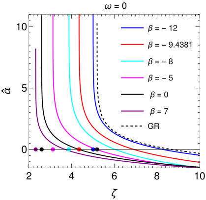
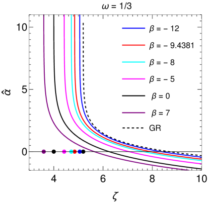
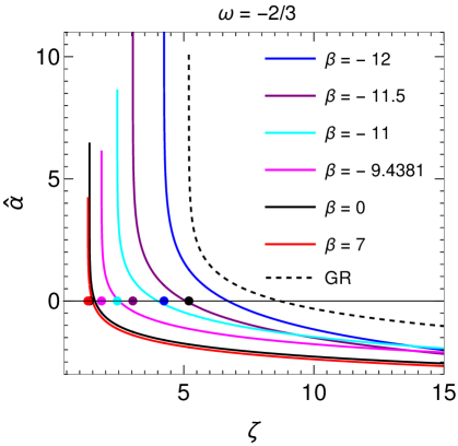
Figure 5: Variations of the deflection angle with the impact parameter $\zeta$ for different values of the model parameter $\beta$ for $\omega=0,$ $1/3$ and $-2/3$ cases respectively, where the black dashed curves represent the Schwarzschild BH. The points on the horizontal axes represent the values of the impact parameter $\zeta=\zeta_{p}$ at which the deflection angle diverges. $M=1$ is taken for all the cases.

From each graphical representation presented in this figure, it is evident that $\hat{\alpha}(\zeta)$ increases as impact parameter $\zeta$ decreases and shows divergence at $\zeta=\zeta_{p}$ as expected. When compared with the Schwarzschild BH, the deflection angle of a minimally coupled $f(R,T)$ gravity BH is found smaller than the Schwarzschild case in all three scenarios. The deflection angle decreases with increasing $\beta$, eventually becoming negative for larger impact parameter values. This negativity is more pronounced for $\beta>0$ whereas for large negative values of $\beta$ i.e., for smaller values of $\beta$ the negativity reduces and the deflection angle approaches to resemble the Schwarzschild behavior beyond some specific impact parameter values. Regarding the negative deflection angle, it is noteworthy that at high impact parameter values photons experience a repulsive interaction with the BH’s gravitational field. Additionally, in the $\omega=-2/3$ case, the deflection angle attains a more negative value compared to the $\omega=0$ and $\omega=1/3$ scenarios and the corresponding $\omega=-2/3$ plot reveals a remarkably negative deflection angle for $\beta>-9.4381$. Moreover, it is seen that for a specific value of $\beta$, a photon exhibits divergence at a larger $\zeta_{p}$ in the $\omega=1/3$ case relative to others. These observations suggest that the gravitational field of a minimally coupled $f(R,T)$ gravity BH surrounded by the radiation field is relatively stronger compared to when it is surrounded by a dust or quintessence field. In fact, the appearance of a negative deflection angle suggests valuable insights into the gravitational behavior of BHs. Several pioneering studies have also highlighted the phenomenon of negative deflection angles in BH spacetime [127, 128, 129, 130, 116].

III.2 Observables

In this subsection we estimate the strong field limit three observables viz., the angular position of the asymptotic relativistic images $\vartheta_{\infty}$, the angular separation between the outermost and asymptotic relativistic images $s$ and the relative magnification of the outermost relativistic image with other relativistic images $r_{mag}$ in the BHs spacetime under consideration. To proceed further, the source and the observer are assumed to be at infinity relative to the BH such that the spacetime curvature impacts the deflection angle close to the lens (BH) only [131, 117]. It is also assumed that the observer, the lens and the source are in perfect alignment along the line of sight (see Fig. 6). This assumption is made because the images appear significantly diminished in size unless the source, lens, and observer are nearly perfectly aligned [65]. The lens equation which relates the positions of the source, observer and lens to the positions of the image can be written as [64, 65, 63]

$$\eta=\vartheta-\frac{d_{ls}}{d_{os}}\,\Delta\alpha_{k},$$ (35)

where $\eta$ and $\vartheta$ are the angular positions of the source and the image respectively from the optic axis, $\Delta\alpha_{k}=\hat{\alpha}-2k\pi$ is an extra deflection angle, $k$ is a positive integer that denotes the total number of complete loops made by a photon around the BHs, and $d_{ls}$ and $d_{os}$ represent the distances of the source and the observer from the lens respectively.

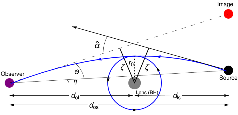
Figure 6: Schematic diagram of the strong field limit gravitational lensing by a BH as a lens.

The position of the $k$th relativistic image $\vartheta_{k}$ in terms of the coefficients $\bar{a}$, $\bar{b}$ and critical impact parameter $\zeta_{p}$ can be derived from equations (30) and (35). Thus, use of the relation $\zeta\approx\vartheta d_{ol}$ in equation (30) yields $\vartheta_{k}$ in the following form [43, 42]:

$$\vartheta_{k}=\vartheta_{k}^{0}+\frac{\zeta_{p}e_{k}(\eta-\vartheta_{k}^{0})d_{os}}{\bar{a}\,d_{ls}d_{ol}},$$ (36)

where $\vartheta_{k}^{0}=\zeta_{p}(1+e_{k})/d_{ol}$ is the relativistic image position associated with deflection angle $\hat{\alpha}=2k\pi$ with $e_{k}=\exp\left({\bar{b}-2k\pi}/\bar{a}\right)$. It is seen that $\vartheta_{k}^{0}$ decreases rapidly with $k$ and in the limit $k\to\infty$, one finds $e_{k}\to 0$, which leads $\vartheta_{\infty}$ to the form as given below [43, 132, 51]:

$$\vartheta_{\infty}=\frac{\zeta_{p}}{d_{ol}}.$$ (37)

Under the assumption of perfect alignment i.e., for $\eta=0$, visibility of relativistic images increases. In this scenario, the geometry of the system is symmetric about the line of sight. Thus, the light emitted from the source can reach the observer after being bent by the gravitational field of the BH along multiple paths in all possible directions [138]. As a result, the distorted image of the source is observed as a circular ring, known as Einstein ring [138, 139]. Taking $d_{os}=2d_{ol}$, the radius of the $k$th relativistic Einstein ring can be obtained from equation (36) as

$$\vartheta_{k}^{E}=\vartheta_{k}^{0}(1-\frac{2\zeta_{p}e_{k}}{\bar{a}\,d_{ol}})=\frac{\zeta_{p}}{d_{ol}}\left(1+e_{k}\right)\left(1-\frac{2\zeta_{p}e_{k}}{\bar{a}\,d_{ol}}\right).$$ (38)

As $d_{ol}\gg\zeta_{p}$, (38) takes the form:

$$\vartheta_{k}^{E}=\frac{\zeta_{p}}{d_{ol}}\left(1+e_{k}\right).$$ (39)

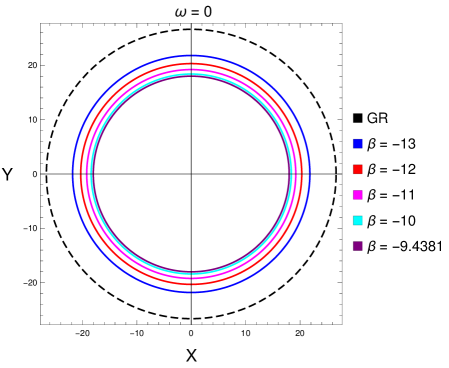
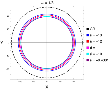
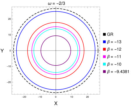
Figure 7: The outermost relativistic Einstein rings for SgrA* by considering it as a minimally coupled $f(R,T)$ BH, for different values of model parameters $\beta$. The left plot is for $\omega=0$, the middle plot is for $\omega=1/3$ and the right one is for $\omega=0$. The black dashed rings correspond to Schwarzschild BHs.

It should be noted that $k=1$ corresponds to the outermost Einstein ring. We depict the outermost Einstein ring of the supermassive BH SgrA* located at the center of the Milky Way, by modeling it as a minimally coupled $f(R,T)$ gravity BH for different values of $\beta$. The mass $M$ and the distance $d_{ol}$ from the Earth of SgrA* are taken as $4.3\times 10^{6}M_{\odot}$ and $8.35$ kpc respectively [93, 92, 140, 142, 141]. The rings are portrayed for $\omega=0$, $\omega=1/3$ and $\omega=-2/3$ separately in Fig. 7, for different values of parameter $\beta$. It is observed that relative to each respective field, the radii of rings decrease as $\beta$ increases.

The magnification of the images serves as another essential source of information. This can be examined from the expression of the magnification of the $k$th relativistic image as given by [63, 43, 50]

$$\mu_{k}=\left.\left(\frac{\eta}{\vartheta}\,\frac{\partial\eta}{\partial\vartheta}\right)^{-1}\right|_{\vartheta_{k}^{0}}\simeq\frac{e_{k}(1+e_{k})d_{os}}{\bar{a}\,\eta\ d_{ls}\ d^{2}_{ol}}\,\zeta^{2}_{p}.$$ (40)

This hints that the magnification decreases rapidly as $k$ increases, thus resulting in the outermost image as the brightest of all the other relativistic images. Also, the presence of the significantly large factor $d^{2}_{ol}$ ensures that the overall luminosity of all images remains relatively weak. Moreover, one would observe a diverging magnification as $\beta\to 0$.

Thus, we can infer that the outermost single loop image $\vartheta_{1}$ is distinguishable from the group of remaining inner images packed as $\vartheta_{\infty}$. Based on this separation the observable $\vartheta_{\infty}$ is obtained as given by equation (37). The other two observables, $s$ and $r_{mag}$, are defined as follows [43, 119, 132, 44]:

$$s =\vartheta_{1}-\vartheta_{\infty}\approx\vartheta_{\infty}\exp\left(\frac{\bar{b}-2\pi}{\bar{a}}\right),$$ (41)

$$r_{\text{mag}} =\frac{\mu_{1}}{\sum_{k=2}^{\infty}\mu_{k}}=\exp\left(\frac{2\pi}{\bar{a}}\right).$$ (42)

Subsequently, we proceed to estimate these three key lensing observables in the strong-field regime, as their evaluation reveals the nature of lensing BHs. To do this, considering the aforementioned mass and distance of SgrA*, the numerical values of the lensing observables $\vartheta_{\infty}$, $s$ and $r_{mag}$ for the BH are computed and summarized in Tables 4 and 5. To analyze their behaviors in the $f(R,T)$ BHs spacetime, the variations of these observables with respect to the modification parameter $\beta$ are illustrated in Fig. 8. It is evident that all three observables decrease with increasing $\beta$ for all three scenarios, $\omega=0$, $\omega=1/3$ and $\omega=-2/3$. For a given $\beta$, the observables attain smaller values in the presence of a dust field compared to a radiation field around it when $\beta\geq-12.23$. Below this critical limit of $\beta$, the values of all three observables exceed those corresponding to the radiation field. Further, $s$ exhibits a relatively steep decline with increasing $\beta$ for $\omega=0$, followed by a very slower variation, whereas for $\omega=1/3$, the decrease is more gradual before showing nearly constant behavior at higher values of $\beta$. On the other hand, for $\omega=-2/3$, although all three observables initially follow a similar trend as in the cases of $\omega=0$ and $\omega=1/3$ from $\beta=-13.7088$, their behavior deviates beyond $\beta\approx-9.8$. Specifically, the observable $\vartheta_{\infty}$ exhibits a sudden decline, while $s$ and $r_{\text{mag}}$ undergo steep growth upto $\beta=-9.4381$. Notably, good results for these observables are obtained only within this range of $\beta$. Consistent with the horizon structure analysis, though not exactly, the observables approach their corresponding GR values at $\beta=-16.7551$, $\beta=-18.8495$ and $\beta=-13.7088$ for the three respective fields and show deviations from GR as $\beta$ increases.

Table 4: Estimation of numerical values of characteristic strong lensing observables by considering supermassive BH SgrA* as a minimally coupled $f(R,T)$ gravity BH for $\omega=0$ and $\omega=1/3$.

	$\omega=0$				$\omega=1/3$
$\beta$	$\vartheta_{\infty}(\mu\text{as})$	s $(\mu\text{as})$	$r_{\text{mag}}$	$\beta$	$\vartheta_{\infty}(\mu\text{as})$	s $(\mu\text{as})$	$r_{\text{mag}}$
SBH	26.5972	0.033239	6.77155	SBH	26.5972	0.033239	6.77155
-16.7551	26.5972	0.033245	6.77155	-18.8495	26.5972	0.033245	6.77155
-13.7088	23.1238	0.020693	6.39666	-13.7088	22.0691	0.017165	6.24005
-12.23	21.1553	0.015319	6.08105	-12.23	21.1155	0.012752	6.07353
-12	20.2849	0.011467	5.90433	-12	20.6717	0.012676	5.98627
-9.4381	17.9771	0.004636	5.26914	-9.4381	19.3424	0.008827	5.68459
-8	17.2371	0.002949	4.97465	-8	18.8598	0.007126	5.54435
0	15.3559	0.001585	3.90956	0	17.4120	0.003259	5.04722
7	14.7449	0.000717	3.37720	7	16.8619	0.002533	4.80724

Table 5: Estimation of numerical values of characteristic strong lensing observables by considering supermassive BH SgrA* as a minimally coupled $f(R,T)$ gravity BH for $\omega=-2/3$.

$\beta$	$\vartheta_{\infty}(\mu\text{as})$	s $(\mu\text{as})$	$r_{\text{mag}}$	$\beta$	$\vartheta_{\infty}(\mu\text{as})$	s $(\mu\text{as})$	$r_{\text{mag}}$
SBH	26.5972	0.033239	6.77155	-11	15.0242	0.001132	3.6522
-13.7088	26.5972	0.041883	6.77592	-10	13.6885	0.000009	2.12064
-12	17.7773	0.004113	5.19698	-9.7	12.5422	0.000425	3.27039
-11.5	16.1008	0.002314	4.41844	-9.4381	9.42328	0.007979	9.14591

     

     

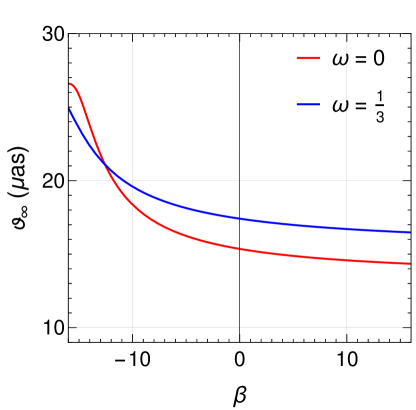
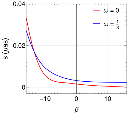
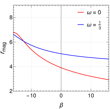
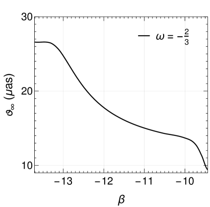
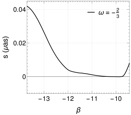
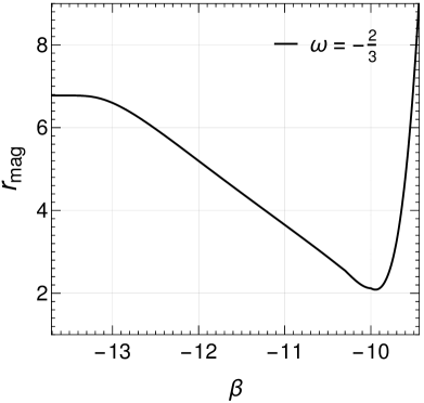
Figure 8: Behaviors of three lensing observables with $\beta.$ The left plot shows the variation of the angular position of the asymptotic relativistic images $\vartheta_{\infty}$, the middle one is for the variation of the angular separation between the outermost and asymptotic relativistic images $s$ and the right plot depicts the variation of relative magnification $r_{mag}$ with $\beta$.

IV Quasinormal Modes of Oscillations

As mentioned earlier the QNMs are the characteristic spacetime oscillations of a BH that occur when its spacetime is being perturbed. QNMs are a reliable tool for diagnosing spacetime near a BH as they provide an important means of probing spacetime with extreme gravity. These are basically complex numbers, with the real part signifying the frequency while the imaginary part signifies the damping of spacetime oscillations.

If we perturb a BH spacetime with a scalar field $\Phi$, in response to which the BH tries to regain its initial state by radiating any deformity in spacetime in the form of gravitational radiation. We describe the probe that couples minimally to $\Phi$ by the following equation of motion [98]:

$$\frac{1}{\sqrt{-g}}\partial_{a}(\sqrt{-g}g^{ab}\partial_{b})\Phi=0.$$ (43)

To obtain the convenient form of this equation, it is essential to express the scalar field $\Phi$ in the spherical form [98]:

$$\Phi(t,r,\theta,\phi)=\exp^{-i\omega t}\frac{\psi(r)}{r}\,Y_{l}^{m}(\theta,\phi),$$ (44)

where $\psi$ is the radial part and $Y_{l}^{m}$ is the spherical harmonics. $\omega$ represents the frequency of oscillation of the temporal part of the wave. Using Eq. (44) into Eq. (43) we finally get the Schrödinger-like wave equation as

$$\frac{d^{2}\psi}{dx^{2}}+(\omega^{2}-V_{l}(x))\psi=0,$$ (45)

where we define $x$ as the tortoise coordinate, given by

$$x=\int\!\frac{dr}{A(r)}.$$ (46)

The potential $V_{l}(r)$ in the BH spacetime is obtained as

$$V_{l}(r)=A(r)\bigg{(}\frac{A^{\prime}(r)}{r}+\frac{l(l+1)}{r^{2}}\Big{)},$$ (47)

where $l$ is the multipole number. For physical consistency, the following boundary conditions are imposed on $\psi(x)$ at the horizon and infinity:

$$\psi(x)\rightarrow\Bigg{\{}\begin{array}[]{ll}\!\!\mathcal{A}\,e^{+i\omega x}&\text{if }x\rightarrow-\infty,\\[3.0pt] \!\!\mathcal{B}\,e^{-i\omega x}&\text{if }x\rightarrow+\infty,\end{array}$$ (50)

where $\mathcal{A}$ and $\mathcal{B}$ denote the constants of integration that behave as amplitudes of waves. With these criteria, we are now in a position to compute the QNMs, for which we follow the Ref. [98]. At this stage it is to be noted that the QNMs associated with a BH spacetime are most often computed using the semi-analytic WKB approximation method as mentioned earlier. However, here we use the 3rd order WKB approximation only due to convergence issues with the higher order as shown in Fig. 9. It is easily observed from the plot that higher order modes are not converging, especially for the multipole $l=1$. Thus, in this work, we compute 2nd, 3rd and 4th order WKB QNMs and then compare the 3rd order results with the time domain QNMs for the sake of accuracy of the computation.

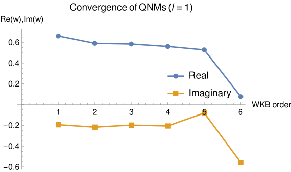
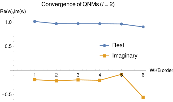
Figure 9: Convergence plots of the different order WKB QNMs of the minimally coupled $f(R,T)$ gravity BHs for $\beta=0.1$. These are applicable for other values of $\beta$ also.

   

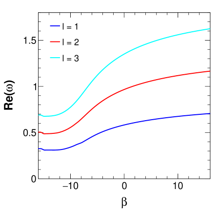
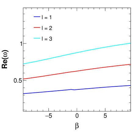
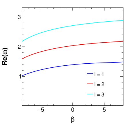
Figure 10: Amplitudes of 3rd order WKB QNMs versus $\beta$ of the minimally coupled $f(R,T)$ BHs for $\omega=0$ (left), $\omega=1/3$ (middle) and $\omega=-2/3$ (right) cases with three values of multipole $l$.

From Fig. 10 it is seen that initially amplitude shows a decreasing trend with the model parameter $\beta$ but it rises as $\beta>-10$ for the case of $\omega=0$. Whereas for the radiation case with $\omega=1/3$, the trend is almost linear, where amplitude increases as the value of parameter $\beta$ increases. A similar situation is observed for the $\omega=-2/3$ case where the amplitude increases with $\beta$ but in a nonlinear fashion. As usual, for higher multipole, we get a larger amplitude in all three cases. Similarly, we plot the damping part of the QNM in Fig. 11. It is seen from the figure that for $\omega=0$, the damping is not stable initially, it decreases a little at the beginning but then starts increasing and again increasing in an irregular manner as $\beta$ is increased. For higher values of $\beta>-8$, it is seen that the damping increases gradually and smoothly which slows down for higher positive values of $\beta$. Further, for higher $l$, the increase in the damping is less compared to lower $l$ with varying degrees depending on the value of $\beta$. For the case of $\omega=1/3$, initially there is a drastic difference in the damping for different $l$, which decreases slightly up to $\beta=-1$. As $\beta$ exceeds $-1$, the damping curves merge very close for all $l$ values and show a smooth increasing pattern with increasing $\beta$. For $\omega=-2/3$, there is a larger variation of damping for $l=1$ compared to the higher multipoles, where the damping initially increases then remains more or less the same with increasing $\beta$ depending on $l$ values.

   

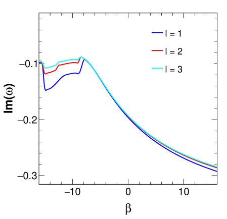
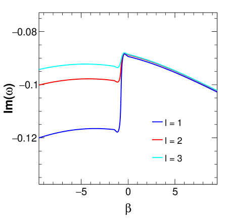
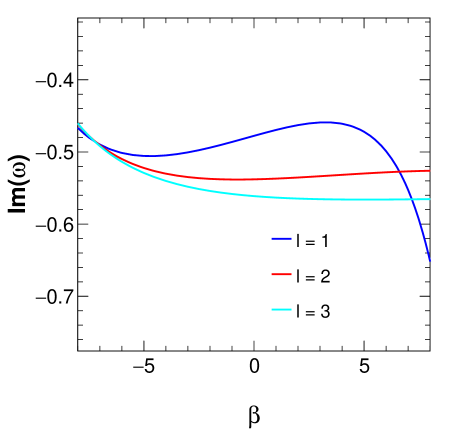
Figure 11: Dampings of 3rd order WKB QNMs versus $\beta$ of the minimally coupled $f(R,T)$ BHs for $\omega=0$ (left), $\omega=1/3$ (middle) and $\omega=-2/3$ (right) cases with three values of multipole $l$.

In Table 6, we tabulate up to 4th order WKB QNMs for the minimally coupled $f(R,T)$ BHs solution (11) along with the associated errors.

Table 6: Up to 4th order WKB QNMs of the BHs solution (11) for $l=1,$ $2$, $n=0$ and for different model parameters $\omega$ and $\beta$. The approximate errors ($\Delta_{3}$) associated with the WKB QNMs have also been computed.

	Multipole	$\omega$	$\beta$	2nd order WKB QNMs	3rd order WKB QNMs	4th order WKB QNMs	$\Delta_{3}$
	Schwarzschild ($l=1$)	-	-	0.294510 -0.107671i	0.291114 -0.098001i	0.292954 -0.097386i	$2.4290\times 10^{-3}$
	$l=1$	$0$	$-16.0$	0.325157 -0.097522i	0.325396 -0.098314i	0.325690 -0.098225i	$3.5643\times 10^{-4}$
		$0$	$-5.0$	0.486328 -0.135807i	0.484093 -0.127572i	0.434974 -0.141978i	$2.3687\times 10^{-2}$
		$0$	$1.0$	0.603433 -0.227997i	0.595620 -0.206432i	0.569958 -0.215726i	$1.7825\times 10^{-2}$
		$0$	$10.0$	0.689967 -0.304221i	0.675111 -0.268832i	0.613410 -0.295873i	$3.6511\times 10^{-2}$
	Schwarzschild ($l=2$)	-	-	0.483977 -0.100560i	0.483211 -0.096805i	0.483647 -0.096718i	$5.4543\times 10^{-4}$
	$l=2$	$0$	$-16.0$	0.502966 -0.096764i	0.503056 -0.097229i	0.503186 -0.097203i	$1.4964\times 10^{-5}$
		$0$	$-5.0$	0.803066 -0.130028i	0.802560 -0.126866i	0.791249 -0.128679i	$5.9403\times 10^{-3}$
		$0$	$1.0$	0.990501 -0.212086i	0.988736 -0.203686i	0.989223 -0.203586i	$1.4987\times 10^{-3}$
		$0$	$10.0$	1.120870 -0.277783i	1.117410 -0.263481i	1.119110 -0.263082i	$2.5806\times 10^{-3}$
	$l=1$	$1/3$	$-9.0$	0.316522 -0.097246i	0.324043 -0.119474i	0.360770 -0.107311i	$2.2634\times 10^{-2}$
		$1/3$	$-5.0$	0.342608 -0.095205i	0.349209 -0.116750i	0.384425 -0.106055i	$2.1598\times 10^{-2}$
		$1/3$	$1.0$	0.384381 -0.097927i	0.382510 -0.090304i	0.343880 -0.100448i	$1.9204\times 10^{-2}$
		$1/3$	$9.0$	0.431236 -0.109279i	0.429426 -0.101899i	0.393538 -0.111192i	$1.7961\times 10^{-2}$
	$l=2$	$1/3$	$-9.0$	0.522599 -0.091364i	0.524122 -0.099710i	0.532904 -0.098066i	$5.6634\times 10^{-3}$
		$1/3$	$-5.0$	0.567216 -0.089682i	0.568563 -0.097839i	0.577116 -0.096389i	$5.4240\times 10^{-3}$
		$1/3$	$1.0$	0.637824 -0.092550i	0.637413 -0.089669i	0.628945 -0.090876i	$4.5136\times 10^{-3}$
		$1/3$	$9.0$	0.714410 -0.104229i	0.714010 -0.101451i	0.706078 -0.102591i	$4.2405\times 10^{-3}$
	$l=1$	$-2/3$	$-6.0$	1.205080 -0.584214i	1.167160 -0.501364i	1.096700 -0.533575i	$5.9806\times 10^{-2}$
		$-2/3$	$-1.0$	1.407960 -0.585178i	1.369780 -0.486179i	1.781360 -0.373849i	$1.4772\times 10^{-1}$
		$-2/3$	$1.0$	1.450180 -0.571179i	1.413240 -0.469531i	2.022270 -0.328126i	$2.4505\times 10^{-1}$
		$-2/3$	$6.0$	1.474860 -0.528203i	1.464650 -0.499012i	2.675790 -0.273145i	$5.6155\times 10^{-1}$
	$l=2$	$-2/3$	$-6.0$	1.778890 -0.549720i	1.766960 -0.509770i	1.756690 -0.512751i	$1.5949\times 10^{-2}$
		$-2/3$	$-1.0$	2.019120 -0.583751i	2.006430 -0.538219i	2.078650 -0.519519i	$2.0389\times 10^{-2}$
		$-2/3$	$1.0$	2.075520 -0.583482i	2.062920 -0.536965i	2.171830 -0.510039i	$3.7469\times 10^{-2}$
		$-2/3$	$6.0$	2.167270 -0.572230i	2.156060 -0.528214i	2.358880 -0.482799i	$8.3120\times 10^{-2}$

As seen from this Table 6, the QNMs are tabulated for the cases of $\omega=0$, i.e. the dust matter case, $\omega=1/3$, i.e. the radiation case and $\omega=-2/3$, i.e. the quintessence case. We also present the QNMs of the Schwarzschild BH for the multipole $l=1$ and $l=2$ for the purpose of comparison. It is seen that the QNMs of the considered $f(R,T)$ BHs have significant deviations from the Schwarzschild case. As already seen from Fig. 10, a common observation is that with increasing multipole, the amplitude increases. Similar is the trend for the parameter $\beta$ where the amplitude shows an increasing trend. The damping part also shows the same trend with respect to $\beta$ as discussed from Fig. 10 analysis. The associated errors have been computed and come out to be in the range of $10^{-5}$ to $10^{-1}$ depending on the value of $\beta$, $l$ and $\omega$. In general, a specific lower value of $\beta=-16$ and higher $l$ values give lower errors. Whereas for $\omega=-2/3$, the errors are maximum. It needs to be mentioned that the error $\Delta_{3}$ is calculated as [25]

$$\Delta_{3}=\frac{W\!K\!B_{4}-W\!K\!B_{2}}{2},$$ (51)

where $W\!K\!B_{2}$ and $W\!K\!B_{4}$ are QNMs calculated respectively from the 2nd and 4th order WKB approximation method.

For the sake of the accuracy of our calculations, we compare the results of QNMs obtained by the WKB method with that of time domain analysis for which we plot the time profile of the wave. The next section deals with the time profile and QNMs computed by a wave fitting algorithm.

V Evolution of a scalar perturbation around the black holes

In this section, we study the evolution of a scalar perturbation around our considered BHs’ spacetime for three different cases: $\omega=0$, $\omega=1/3$ and $\omega=-2/3$. We use the time domain integration method to study this evolution. For this, we follow the method described in Refs. [133, 134]. Thus, considering $\psi(x,t)=\psi(i{\Delta}x,j{\Delta}t)=\psi_{i,j}$ and $V(r(x))=V(x,t)=V_{i,j}$, the equation (43) can be expressed in the following form:

$$\frac{\psi_{i+1,j}-2\psi_{i,j}+\psi_{i-1,j}}{{\Delta}x^{2}}-\frac{\psi_{i,j+1}-2\psi_{i,j}+\psi_{i,j-1}}{{\Delta}t^{2}}-V_{i}\psi_{i,j}=0.$$ (52)

This equation can be rewritten as

$$\psi_{i,j+1}=-\,\psi_{i,j-1}+\left(\frac{{\Delta}t}{{\Delta}x}\right)^{\!2}\!\!(\psi_{i+1,j}+\psi_{i-1,j})+\left(2-2\,\left(\frac{{\Delta}t}{{\Delta}x}\right)^{\!2}-V_{i}\Delta{t}^{2}\right)\!\psi_{i,j}.$$ (53)

Here, we use initial conditions as $\psi(x,t)=\exp\left[-(x-\mu)^{2}/2{\sigma}^{2}\right]$ and $\left.\psi(x,t)\right|_{t<0}=0$, where $\mu$ is the median and $\sigma$ is the width of the initial wave packet. Further, we use the Von Neumann stability condition $\frac{{\Delta}t}{{\Delta}x}\!<\!1$ for stability of results and calculate the time profiles.

     

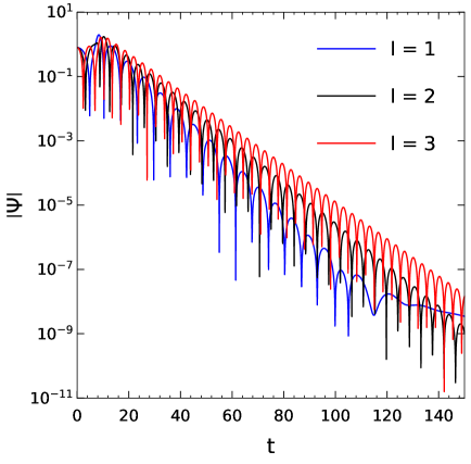
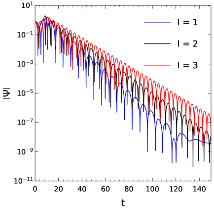
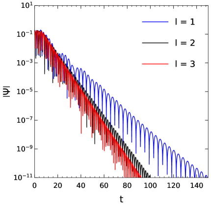
Figure 12: Time domain profile for the scalar perturbation in the spacetime of the minimally coupled $f(R,T)$ BHs. The left plot is for $\omega=0$ and $\beta=-8.8$, the right plot is for $\omega=1/3$ and $\beta=-6$, and the bottom plot is for $\omega=-2/3$ and $\beta=-2$.

In Fig. 12 we plot the time domain profiles for $\omega=0$, $\omega=1/3$ and $\omega=-2/3$ in the unit of $M$. It can be observed from the figure that the pattern of variation of the time domain profile with the multipole $l$ is in agreement with the results obtained from the 3rd order WKB approximation method.

     

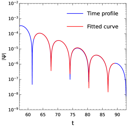
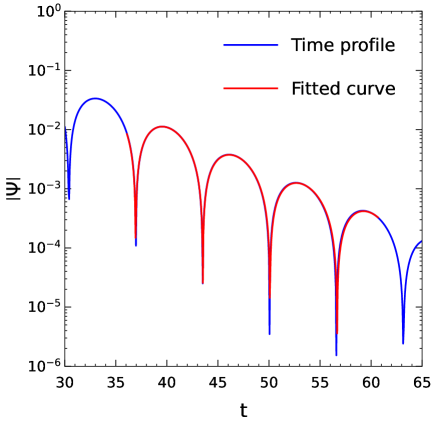
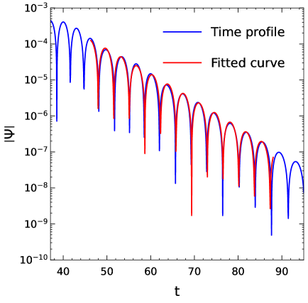
Figure 13: Fitting of the time domain profile to estimate the QNMs as an example for $l=1$. The left plot is for $\omega=0$, $\beta=-8.8$, the right plot is for $\omega=1/3$, $\beta=-6$ and the bottom plot is for $\omega=-2/3$, $\beta=-2$.

Fig. 13 shows the fitting of the time domain profiles using the Levenberg Marquardt algorithm [135, 136, 137]. From the fitting, we calculate the QNMs of the BHs. Further, we calculate the difference in the magnitudes of the QNMs obtained from the 3rd order WKB approximation method and those obtained from the time domain analysis method as follows:

$$\Delta_{Q\!N\!M}=\frac{\left|QNM_{\text{WKB}}-QNM_{\text{Time domain}}\right|}{2}.$$ (54)

Table 7 shows the calculated QNMs of the BHs for $\omega=0$ with $\beta=-8.8$, $\omega=1/3$ with $\beta=-6$, and $\omega=-2/3$ with $\beta=-2$ respectively.

Table 7: QNMs of the minimally coupled $f(R,T)$ gravity BHs computed from the fitting of the time domain profiles using the Levenberg Marquardt algorithm [135, 136, 137] in comparison with that obtained from 3rd order WKB approximation method for different values of $\omega$ and $\beta$.

	$\omega$	$\beta$	Multipole $l$	3rd order WKB QMNs	Time domain QNMs	$R^{2}$	$\Delta_{Q\!N\!M}$
	$\omega=0$	$\beta=-8.8$	$1$	$0.371088-0.116790i$	$0.371218-0.118280i$	0.995280	$2.818530\times 10^{-4}$
			$2$	$0.606594-0.098307i$	$0.602417-0.097901i$	0.985772	$2.093900\times 10^{-3}$
			$3$	$0.846850-0.092873i$	$0.842375-0.091867i$	0.988405	$2.278800\times 10^{-3}$
	$\omega=1/3$	$\beta=-6$	$1$	$0.333450-0.087057i$	$0.324891-0.149260i$	0.981999	$6.455010\times 10^{-3}$
			$2$	$0.554941-0.086645i$	$0.522741-0.095422i$	0.987519	$1.514250\times 10^{-2}$
			$3$	$0.775963-0.086548i$	$0.723183-0.091149i$	0.989405	$2.593500\times 10^{-2}$
	$\omega=-2/3$	$\beta=-2$	$1$	$1.341550-0.494087i$	$1.343261-0.472752i$	0.971959	$2.808810\times 10^{-3}$
			$2$	$1.972000-0.537327i$	$1.971946-0.516896i$	0.989519	$2.664080\times 10^{-3}$
			$3$	$2.635360-0.554069i$	$2.635490-0.554137i$	0.989134	$7.061500\times 10^{-5}$

From this time domain analysis we have seen that the QNMs obtained from this analysis are in good agreement with the results obtained from the WKB approximation method. As the $R^{2}$s for the fits are also found to be satisfactory, the accuracy of the fittings is ensured.

VI Conclusion

Gravitational lensing is a versatile technique for exploring the properties of spacetime and for testing the predictions of different theories of gravity. In the first part of this study, we have analyzed the strong gravitational lensing properties of BHs described by the $f(R,T)$ gravity theory, focusing on a minimally coupled model of the theory. The analysis has relied on a strong field limit universal method developed by V. Bozza, applicable to all spacetime in any gravity theory where the photons follow the standard geodesic equations [43]. We have conducted the analysis considering three types of surrounding fields around the BHs, namely the dust field, the radiation field and the quintessence field. Here, we have concentrated on the investigation of the characteristics of the region just outside the event horizon of the minimally coupled $f(R,T)$ gravity BHs for these fields separately through the analysis of photon deflection extremely close to the photon sphere of the BHs. For this, the influence of the model parameter $\beta$ on different photon trajectories is examined. Our analysis reveals that the lensing coefficients $\bar{a}$ and $\bar{b}$ exhibit distinct and contrasting behaviors with $\beta$ depending on the values of $\omega$. These variations directly affect the deflection angle $\hat{\alpha}$ which decreases with increasing impact parameter $\zeta$ and becomes negative for larger values of $\zeta$, highlighting repulsive interactions by the gravitational field of the BHs. Furthermore, by considering the supermassive BH SgrA* as a minimally coupled $f(R,T)$ gravity BH, we have computed the numerical values of the lensing observables. The computed lensing observables: the angular position of relativistic images $\vartheta_{\infty}$, angular separation $s$, and relative magnification $r_{\text{mag}}$ demonstrate a consistent decline with increasing $\beta$ in scenarios with $\omega=0$ and $\omega=1/3$. Remarkably, when comparing the observables of the first two classes of BHs, the respective observables are found smaller in a dust dominated environment than in the presence of the radiation field, except for $\beta\leq-12.23$, in which a sudden growth of dust field observables is noticed. This sudden increase of observables could be due to the dominance of the physical parameters linked to the dust field over those of the radiation field beyond this value. In addition, the analysis for $\omega=-2/3$ reveals a distinct deviation in the behavior of the observables beyond $\beta\approx-9.8$ in contrast to the cases of $\omega=0$ and $\omega=1/3$. The sudden decline of $\vartheta_{\infty}$ and the steep growth of $s$ and $r_{mag}$ up to $\beta=-9.4381$ indicate a significant dependence of the observables on the parameter $\beta$. These results highlight that reliable predictions for the observables are confined within this specific range of $\beta$, emphasizing the intricate relationship between $\beta$ and the underlying physical properties of the system. However, our findings underscore the significant role of $\beta$ and the type of surrounding field in shaping the strong lensing behavior of the considered BHs spacetime with deviation limits $\beta=-16.7551$ in $\omega=0$ case, $\beta=-18.8495$ in $\omega=1/3$ and $\beta=-13.7088$ for $\omega=-2/3$, from GR. Indeed, prominent deviation is observed as $\beta$ increases providing a potential avenue for testing deviations from GR through strong lensing observations.

The QNMs associated with the BHs’ spacetime have also been studied. For three values of equation of state parameter $\omega$, we calculated the QNMs of BHs using the 3rd order WKB approximation method as the higher order ($>$ 5th order) values of QNMs of the BHs obtained by this method are not converging. We plot the real part of calculated QNMs denoting the amplitude of frequency of the mode against the model parameter $\beta$. It is seen that the amplitude increases with increasing $\beta$ for all three cases. For the imaginary part of the QNMs denoting damping rate, we found that for $\omega=-2/3$, the highest damping has been observed compared to the other two cases. For $\omega=1/3$, the plots converse near $\beta=0$ and then show a steady increase in damping as $\beta$ increases. Time evolution of the QNMs of oscillations has also been studied and the decaying modes are clearly visible from their profiles. For the sake of accuracy, we have compared the results obtained by the WKB method with that obtained from the time profile fitting method based on the Levenberg Marquardt algorithm and found a good agreement in results as shown in Table 7. The deviation between the results of these two methods has been represented via a quantity parameter $\Delta_{Q\!N\!M}$ defined in equation (54), which comes out to be of the order of about $10^{-3}$, thus signifying a good match between the two methods.

We hope that this work will contribute towards a better understanding of the nature of GWs and the lensing phenomena in MTGs. This study enriches our understanding of BH spacetimes in MTGs and offers valuable insights for future observational and theoretical investigations in astrophysics.

References

- [1] B. P. Abbott et al., Observation of Gravitational Waves from a Binary Black Hole Merger, Phys. Rev. Lett. 116, 061102 (2016).
- [2] B. P. Abbott et al., Observation of Gravitational Waves from a 22-Solar-Mass Binary Black Hole Coalescence, Phys. Rev. Lett. 116, 241103 (2016).
- [3] B. P. Abbott et al., Observation of Gravitational Waves from a Binary Neutron Star Inspiral, Phys. Rev. Lett. 119, 161101 (2017).
- [4] B. P. Abbott et al., Observation of a Binary-Black-Hole Coalescence with Asymmetric Masses, Phys. Rev. D 102, 043015 (2020).
- [5] R. Abbott et al., Observation of Gravitational Waves from Two Neutron Star–Black Hole Coalescences, ApJL 915, L5 (2021).
- [6] R. Abbott et al., Search for continuous gravitational wave emission from the Milky Way center in O3 LIGO-Virgo data, Phys. Rev. D 106, 042003 (2022).
- [7] Event Horizon Telescope Collaboration et al., First M87 Event Horizon Telescope Results. I. The Shadow of the Supermassive Black Hole, APJL 875, L1 (2019).
- [8] Event Horizon Telescope Collaboration et al., First M87 Event Horizon Telescope Results. II. Array and Instrumentation, APJL 875, L2 (2019).
- [9] Event Horizon Telescope Collaboration et al., First M87 Event Horizon Telescope Results. III. Data Processing and Calibration, APJL 875, L3 (2019).
- [10] Event Horizon Telescope Collaboration et al., First M87 Event Horizon Telescope Results. IV. Imaging the Central Supermassive Black Hole, APJL 875, L4 (2019).
- [11] Event Horizon Telescope Collaboration et al., First M87 Event Horizon Telescope Results. V. Physical Origin of the Asymmetric Ring, APJL 875, L5 (2019).
- [12] Event Horizon Telescope Collaboration et al., First M87 Event Horizon Telescope Results. VI. The Shadow and Mass of the Central Black Hole, APJL 875, L6 (2019).
- [13] R. A. Konoplya and A. Zhidenko, Solutions of the Einstein equations for a black hole surrounded by a galactic halo, Astrophys. J. 933, 166 (2022).
- [14] R. A. Konoplya and A. F. Zinhailo, Hawking radiation of non-Schwarzschild black holes in higher derivative gravity: a crucial role of grey-body factors, Phys. Rev. D 99, 014060 (2019).
- [15] E. Berti, V. Cardoso and A. O. Starinets, Quasinormal modes of black holes and black branes, Class. Quant. Grav. 26, 163001 (2009).
- [16] C. M. Will, The confrontation between General Relativity and Expermient, Living Reviews in Relativity 17, 4 (2014).
- [17] R. Karmakar and U. D. Goswami, Quasinormal modes, thermodynamics and shadow of black holes in Hu–Sawicki gravity theory, EPJC 84, 969 (2024).
- [18] K. S. Stelle, Renormalization of higher-derivative quantum gravity, Phys. Rev. D 16, 953 (1977).
- [19] Riess et al., Observational Evidence from Supernovae for an Accelerating Universe and a Cosmological Constant, The Astronomical Journal 116, 1009 (1998).
- [20] Perlmutter et al., Measurements of and from 42 high-redshift supernovae, Astrophys. J. 517, 556 (1999).
- [21] N. A. Bahcall, J. P. Ostriker, S. Perlmutter and P. J. Steinhardt, The cosmic triangle: Revealing the state of the universe, Science 284, 5419 (1999).
- [22] Carpil et al., Quantum Gravity: A Brief History of Ideas and Some Prospects, IJMPD 24, 1530028 (2015).
- [23] R. Karmakar, D. J. Gogoi and U. D. Goswami, Thermodynamics and shadows of GUP-corrected black holes with topological defects in Bumblebee gravity, Phys. Dark Universe 41, 101249 (2023).
- [24] D. J. Gogoi, R. Karmakar and U. D. Goswami, Quasinormal modes of nonlinearly charged black holes surrounded by a cloud of strings in Rastall gravity, IJGMMP 20, 2350007 (2023).
- [25] R. Karmakar and U. D. Goswami, Quasinormal modes, temperatures and greybody factors of black holes in a generalized Rastall gravity theory, Phys. Scrr 99, 055003 (2024).
- [26] A. A. Starobinsky, The Perturbation Spectrum Evolving from a Nonsingular Initially De-Sitter Cosmology and the Microwave Background Anisotropy, Sov. Astron. Lett. 9, 302 (1983).
- [27] W. Hu, I. Sawicki, Models of f(R) Cosmic Acceleration that Evade Solar-System Tests, Phys. Rev. D 76, 064004,2007
- [28] D. J. Gogoi and U. D. Goswami, A new gravity model and properties of gravitational waves in it, EPJC 80, 1101 (2020).
- [29] T. Harko, F. S. N. Lobo, S. Nojiri and S. D. Odintsov, gravity, Phys. Rev. D 84, 024020 (2011).
- [30] P. S. Singh and K. P. Singh, Gravity model behaving as a dark energy source, New Astronomy 84, 101542 (2021).
- [31] H. Shabani, A. De, T. H. Loo and E. N. Saridakis, Cosmology of f(Q) gravity in non-flat Universe , EPJC 84, 285 (2024).
- [32] P. Sarmah, A. De and U. D. Goswami, Anisotropic LRS-BI Universe with gravity theory, Phys. Dark Universe 40, 101209 (2023).
- [33] P. Rastall, Generalization of the Einstein Theory, Phys. Rev. D 6, 3357 (1972).
- [34] F. Darabi, H. Moradpour, I. Licata, Y. Heydarzade and C. Corda, Einstein and Rastall Theories of Gravitation in Comparison, EPJC 78, 25 (2018).
- [35] F. S. N. Lobo and T. Harko, Extended theories of gravity, The Thirteenth Marcel Grossmann Meeting pp, 1164-1166 (2015).
- [36] A. Einstein, The Foundation of the General Theory of Relativity, Ann. Phys. (N.Y.) 49, 769 (1916); 14, 517 (2005).
- [37] M. Bartelmann, Gravitational Lensing, Class. Quan. Grav. 27, 233001 (2010).
- [38] J. Wambsganss, Gravitational Lensing in Astronomy, Living Rev. Relativ. 1, 12 (1998).
- [39] R. D. Blandford and R. Narayan, Cosmological Applications of Gravitational Lensing, Annu. Rev. Astron. Astrophys. 30, 311 (1992).
- [40] A. B. Congdon and C. R. Keeton, Principles of Gravitational Lensing: Light Deflection as a Probe of Astrophysics and Cosmology, Springer International Publishing, Cham (2018).
- [41] F. W. Dyson, et al., IX. A determination of the deflection of light by the sun’s gravitational field, from observations made at the total eclipse of May 29, 1919, Phil. Trans. R. Soc. A 220, 291 (1920).
- [42] J. Kumar and S. U. Islam and S. G. Ghosh, Investigating strong gravitational lensing effects by supermassive black holes with Horndeski gravity, EPJC 82, 443 (2022).
- [43] V. Bozza, Gravitational lensing in the strong field limit, Phys. Rev. D 66, 103001 (2002).
- [44] S. S. Zhao and Y. Xie, Strong Deflection Gravitational Lensing by a Modified Hayward Black Hole, EPJC 77, 272 (2017).
- [45] C. G. Darwin, The Gravity Field of a Particle, Proc. R. Soc. Lond. A 249, 180 (1959).
- [46] D. Clowe et al., A Direct Empirical Proof of the Existence of Dark Matter, ApJ 648, L109 (2006).
- [47] R. Massey, T. Kitching, and J. Richard, The Dark Matter of Gravitational Lensing, Rep. Prog. Phys. 73, 086901 (2010).
- [48] Z. Fu and S. Gao, The Application of Gravitational Lensing on Observation of Dark Matter Candidates, J. Phys.: Conf. Ser. 2386, 012076 (2022).
- [49] V. Bozza, Quasiequatorial Gravitational Lensing by Spinning Black Holes in the Strong Field Limit, Phys. Rev. D 67, 103006 (2003).
- [50] R. Whisker, Strong Gravitational Lensing by Braneworld Black Holes, Phys. Rev. D 71, 064004 (2005).
- [51] S. Chen and J. Jing, Strong Field Gravitational Lensing in the Deformed Hořava-Lifshitz Black Hole, Phys. Rev. D 80, 024036 (2009).
- [52] Y. Liu, S. Chen, and J. Jing, Strong Gravitational Lensing in a Squashed Kaluza-Klein Black Hole Spacetime, Phys. Rev. D 81, 124017 (2010).
- [53] C. Ding et al., Strong Gravitational Lensing in a Noncommutative Black-Hole Spacetime, Phys. Rev. D 83, 084005 (2011).
- [54] H. Sotani and U. Miyamoto, Strong Gravitational Lensing by an Electrically Charged Black Hole in Eddington-Inspired Born-Infeld Gravity, Phys. Rev. D 92, 044052 (2015).
- [55] N. Tsukamoto, Affine Perturbation Series of the Deflection Angle of a Ray near the Photon Sphere of a Reissner-Nordström Black Hole, Phys. Rev. D 106, 084025 (2022).
- [56] N. Tsukamoto, Gravitational Lensing by Using the 0th Order of Affine Perturbation Series of the Deflection Angle of a Ray near a Photon Sphere, EPJC 83, 284 (2023).
- [57] A. Chowdhuri, S. Ghosh, and A. Bhattacharyya, A Review on Analytical Studies in Gravitational Lensing, Front. Phys. 11, 1113909 (2023).
- [58] A. R. Soares et al., Holonomy Corrected Schwarzschild Black Hole Lensing, Phys. Rev. D 108, 124024 (2023).
- [59] G. Mustafa and S. K. Maurya, Testing Strong Gravitational Lensing Effects of Various Supermassive Compact Objects for the Static and Spherically Symmetric Hairy Black Hole by Gravitational Decoupling, EPJC 84, 686 (2024).
- [60] V. Bozzaa and G. Scarpettaa, Strong deflection limit of black hole gravitational lensing with arbitrary source distances, Phys. Rev. D 76, 083008 (2007).
- [61] H. C. Ohanian, The black hole as a gravitational “lens”, Am. J. Phys. 55, 428 (1987)
- [62] R. J. Nemiro, Visual distortions near a neutron star and black hole, Am. J. Phys. 61, 619 (1993)
- [63] V. Bozza, S. Capozziello, G. Iovane and G. Scarpetta, Strong Field Limit of Black Hole Gravitational Lensing, Gen. Rel. Grav. 33, 1535 (2001).
- [64] K. S. Virbhadra, D. Narasimha1 and S. M. Chitre, Role of the scalar field in gravitational lensing, A&A337, 1 (1998).
- [65] K. S. Virbhadra and G. F. R. Ellis, Schwarzschild black hole lensing, Phys. Rev. D 62, 084003 (2000).
- [66] K. S. Virbhadra, Relativistic Images of Schwarzschild Black Hole Lensing, Phys. Rev. D 79, 083004 (2009).
- [67] K. S. Virbhadra, Distortions of Images of Schwarzschild Lensing, Phys. Rev. D 106, 064038 (2022).
- [68] E. F. Eiroa, G. E. Romero and D. F. Torres, Reissner-Nordstrom black hole lensing, Phys. Rev. D 66, 024010, (2002).
- [69] E. F. Eiroa and C. M. Sendra, Gravitational lensing by a regular black hole, Class. Quan. Grav. 28, 085008 (2011).
- [70] V. Perlick, On the exact gravitational lens equation in spherically symmetric and static spacetimes, Phys. Rev. D 69, 064017 (2004).
- [71] S. Wang, S. Chen and J. Jing, Strong gravitational lensing by a Konoplya-Zhidenko rotating non-Kerr compact object, JCAP 11, 020 (2016).
- [72] C. R. Keeton and A. O. Petters, Formalism for Testing Theories of Gravity Using Lensing by Compact Objects. I: Static, Spherically Symmetric Case, JCAP 72,104006 (2005).
- [73] G. J. Olmo et al., Shadows and photon rings of regular black holes and geonic horizonless compact objects, Class. Quant. Grav. 40, 174002 (2023).
- [74] F. Atamurotov and S. G. Ghosh, Gravitational Weak Lensing by a Naked Singularity in Plasma, Eur. Phys. J. Plus 137, 662 (2022).
- [75] Y. Chen et al., Gravitational Lensing by Born-Infeld Naked Singularities, Phys. Rev. D 109, 084014 (2024).
- [76] M. K. Hossain et al., Gravitational Deflection of Massive Body around Naked Singularity, Nucl. Phys. B 1005, 116598 (2024).
- [77] R. Shaikh et al., Strong Gravitational Lensing by Wormholes, JCAP 2019, 028 (2019).
- [78] S. Kumar, A. Uniyal, and S. Chakrabarti, Shadow and Weak Gravitational Lensing of Rotating Traversable Wormhole in Nonhomogeneous Plasma Spacetime, Phys. Rev. D 109, 104012 (2024).
- [79] N. Godani and G. C. Samanta, Gravitational Lensing for Wormhole with Scalar Field in f(R) Gravity, IJGMMP 20, 2350075 (2023).
- [80] R. Shaikh and S. Kar, Gravitational lensing by scalar-tensor wormholes and the energy conditions, Phys. Rev. D 96, 044037 (2017).
- [81] S. Kalita, S. Bhatporia, and A. Weltman, Gravitational Lensing in Modified Gravity: A Case Study for Fast Radio Bursts, J. Cosmol. Astropart. Phys. 2023, 059 (2023).
- [82] F. B. Davies et al., Constraining the Gravitational Lensing of z 6 Quasars from Their Proximity Zones, ApJL 904, L32 (2020).
- [83] R. C. Pantig and A. Övgün, Dark Matter Effect on the Weak Deflection Angle by Black Holes at the Center of Milky Way and M87 Galaxies, EPJC 82, 391 (2022).
- [84] R. A. Konoplya, Shadow of a black hole surrounded by dark matter, Phys. Letts. B 795, 1 (2019).
- [85] G. J Olmo et al., Shadows and photon rings of regular black holes and geonic horizonless compact objects, Class. Quant. Grav. 40, 174002 (2023).
- [86] W. Javed et al., Weak Deflection Angle by Kalb–Ramond Traversable Wormhole in Plasma and Dark Matter Mediums, Universe 8, 599 (2022).
- [87] A. R. Soares, R. L. L. Vitória, and C. F. S. Pereira, Gravitational Lensing in a Topologically Charged Eddington-Inspired Born–Infeld Spacetime, EPJC 83, 903 (2023).
- [88] N. Parbin, D. J. Gogoi, and U. D. Goswami, Weak Gravitational Lensing and Shadow Cast by Rotating Black Holes in Axionic Chern–Simons Theory, Phys. Dark Univ. 41, 101265 (2023).
- [89] S. S. Zhao and Y. Xie, Strong Field Gravitational Lensing by a Charged Galileon Black Hole, JCAP 2016, 007 (2016).
- [90] S. U. Islam, J. Kumar, and S. G. Ghosh, Strong Gravitational Lensing by Rotating Simpson-Visser Black Holes, J. Cosmol. Astropart. Phys. 2021, 013 (2021).
- [91] G. W. Gibbons and M. C. Werner, Applications of the Gauss-Bonnet Theorem to Gravitational Lensing, Class. Quan. Grav. 25, 235009 (2008).
- [92] Y. Dong, The Gravitational Lensing by Rotating Black Holes in Loop Quantum Gravity, Nucl. Phys. B 1005, 116612 (2024).
- [93] X. M. Kuang et al., Constraining a Modified Gravity Theory in Strong Gravitational Lensing and Black Hole Shadow Observations, Phys. Rev. D 106, 064012 (2022).
- [94] X. J. Gao et al, Investigating strong gravitational lensing with black hole metrics modified with an additional term, Phys. Lett. B 822, 136683 (2021).
- [95] A. Övgün, G. Gyulchev, and K. Jusufi, Weak Gravitational Lensing by Phantom Black Holes and Phantom Wormholes Using the Gauss-Bonnet Theorem, Annals of Physics 406, 152 (2019).
- [96] J. Badía and E. F. Eiroa, Gravitational Lensing by a Horndeski Black Hole, EPJC 77, 779 (2017).
- [97] S. G. Ghosh, R. Kumar, S. U. Islam, Parameters estimation and strong gravitational lensing of nonsingular Kerr-Sen black holes, JCAP 03, 056 (2021).
- [98] R. A. Konoplya and A. Zhidenko, Quasinormal modes of black holes: From astrophysics to string theory, Rev. Mod. Phys. 83, 793 2011.
- [99] R. Karmakar and U. D. Goswami, Quasinormal modes and thermodynamic properties of GUP-corrected schwarzschild black hole surrounded by quintessence, IJMPA 37, 2250180 (2022).
- [100] C. V. Vishveshwara, Stability of the Schwarzschild metric, Phys. Rev. D 1, 2870 (1970).
- [101] S. Chandrasekhar and S. Detweiler, The quasi-normal modes of the Schwarzschild black hole, Proc. R. Soc. Lond. A, Math. Phys. Sci. 344, 1639 (1975).
- [102] B. F. Schutz and C. M. Will, Black hole normal modes - A semianalytic approach, Astrophys. J 291, L33 (1985).
- [103] R. A. Konoplya, A. Zhidenko and A. F. Zinhailo, Higher order WKB formula for quasinormal modes and grey-body factors: recipes for quick and accurate calculations, Class. Quantum Grav. 36, 155002 (2019).
- [104] A. Al-Badawi, Quazinormal modes and greybody factor of black hole surrounded by a quintessence in the S-V-T modified gravity as well as shadow, Phys. Scr. 99, 065002 (2024).
- [105] J. W. Moffat, Black Holes in Modified Gravity (MOG), EPJC 75, 175 (2015).
- [106] L. C. N. Santos et al., Kiselev black holes in f(R,T) gravity, Gen. Rel. Grav. 55, 94 (2023).
- [107] B. Hazarika, P. Phukon, Thermodynamic Properties and Shadows of Black Holes in f(R,T) Gravity, [arXiv.2410.00606].
- [108] T. Harko, F. S. N. Lobo, S. Nojri, S. D. Odintsov, f(R,T) gravity, Phys. Rev. D 84, 024020 (2011).
- [109] F. G. Alvarenga, M. J. S. Houndjo, A. V. Monwanou and J. B. Chabi Orou, Testing some f(R,T) gravity models from energy conditions, J. Mod. Phys. 4, 130 (2013).
- [110] H. Shabani and M. Farhoudi, Cosmological and Solar System Consequences of f(R,T) Gravity Models, Phys. Rev. D 90, 044031 (2014).
- [111] H. Shabani and M. Farhoudi, f(R,T) Cosmological Models in Phase Space,Phys. Rev. D 88, 044048 (2013).
- [112] V. V. Kiselev, Quintessence and black holes, Class. Quant. Grav. 20, 1187 (2003).
- [113] D. Deb et al., Exploring physical features of anisotropic strange stars beyond standard maximum mass limit in f(R,T) gravity, MNRAS 000, (2018).
- [114] S. Weinberg, Gravitation and Cosmology: Principles and Applications of the General Theory of Relativity, John Wiley Sons, New York, (1972).
- [115] N. Tsukamotoand, Deflection angle in the strong deflection limit in a general asymptotically flat, static, spherically symmetric spacetime, Phys. Rev. D 95, 064035 (2017).
- [116] G Mohan, N. Parbin and U. D. Goswami, Investigating the effects of gravitational lensing by Hu-Sawicki f(R) gravity black holes, [//doi.org/10.48550/arXiv.2411.19048].
- [117] S. U. Islam, S. G. Ghosh and S. D. Maharaj, Strong gravitational lensing by Bardeen black holes in 4D EGB gravity:constraints from supermassive black holes, Chi. J .Phys. 89, 1710 (2024).
- [118] S. Chandrasekhar, The Mathematical Theory of Black Holes, Oxford Univ. Press, New York.
- [119] S. U. Islam, R. Kumar and S. G. Ghosh, Gravitational lensing by black holes in the 4D Einstein-Gauss-Bonnet gravity, JCAP 09, 030 (2020).
- [120] Y. Wang et al., Strong Gravitational Lensing by Static Black Holes in Effective Quantum Gravity, [arXiv:2410.12382v1].
- [121] C. -M. Clarissa, K. S. Virbhadra and G. F. R. Ellis, The geometry of photon surfaces, J. Math. Phys 42, 818 (2000).
- [122] K. S. Virbhadra, D. Narasimha and S. M. Chitre, Role of the scalar field in gravitational lensing, Astron. Astrophys. 1, 337 (1998).
- [123] S. Weinberg, Gravitation and Cosmology: Principles and Applications of the General Theory of Relativity, John Wiley & Sons, New York, (1972).
- [124] R. Zhang, J. Jing and S. Chen, Strong gravitational lensing for black holes with scalar charge in massive gravity, Phys. Rev. D 95, 064054 (2017).
- [125] S. Chen and J. Jing, Strong gravitational lensing by a rotating non-Kerr compact object, Phys. Rev. D 85, 124029 (2012).
- [126] R. Kumar, S. U. Islam, and S. G. Ghosh, Gravitational Lensing by Charged Black Hole in Regularized 4D Einstein–Gauss-Bonnet Gravity, EPJC 80, 1128 (2020).
- [127] N. Parbin et al., Deflection Angle, Quasinormal Modes and Optical Properties of a de Sitter Black Hole in f(T,B) Gravity, Phys. Dark Univ. 42, 101315 (2023).
- [128] S. Panpanich, S. Ponglertsakul, and L. Tannukij, Particle Motions and Gravitational Lensing in de Rham-Gabadadze-Tolley Massive Gravity Theory, Phys. Rev. D 100, 044031 (2019).
- [129] K. Nakashi et al., Null Geodesics and Repulsive Behavior of Gravity in D Massive Gravity, Prog. Theor. Exp. Phys. 2019, 073E02 (2019).
- [130] T. Kitamura, K. Nakajima, and H. Asada, Demagnifying Gravitational Lenses toward Hunting a Clue of Exotic Matter and Energy, Phys. Rev. D 87, 027501 (2013).
- [131] V. Bozza, Gravitational Lensing by Black Holes, Gen. Rel. Grav. 42, 2269 (2010).
- [132] J. R. Nascimento, A. Yu. Petrov, P. J. Porfírio and A. R. Soares, Gravitational lensing in black-bounce spacetime, Phys. Rev. D. 102, 044021 (2020).
- [133] D. Gogoi and U. Goswami, Quasinormal modes and Hawking radiation sparsity of GUP corrected black holes in bumblebee gravity with topological defects, JCAP 06, 029, 2022.
- [134] C.Gundlach et al., Late-time behavior of stellar collapse and explosions. II. Nonlinear evolution, Phys. Rev. D 49, 890 (1994).
- [135] K. Levenberg, A method for the solution of certain non-linear problems in least squares Quart. Appl. Math.2 168 (1944).
- [136] D. W. Marquardt, An Algorithm for Least-Squares Estimation of Nonlinear Parameters J. Soc. Indust. Appl. Math. 11, 431 (1963).
- [137] E. Berti et al., Mining information from binary black hole mergers: A comparison of estimation methods for complex exponentials in noise, Phys. Rev. D 75, 124017 (2007).
- [138] R. K. Walia, Observational Predictions of LQG Motivated Polymerized Black Holes and Constraints From Sgr A* and M87*, JCAP 03, 029 (2023).
- [139] V. Bozza and L. Mancini, Gravitational Lensing by Black Holes: a comprehensive treatment and the case of the star S2, Astrophys.J. 611, 1045 (2004).
- [140] A. M. Ghez et. al., Measuring Distance and Properties of the Milky Way’s Central Supermassive Black Hole with Stellar Orbits, APJ 689, 1044 (2008).
- [141] S. Gillessen et. al., Monitoring stellar orbits around the massive black hole in the galactic center, APJ 692, 1075 (2009).
- [142] T. Do et al., Relativistic redshift of the star S0-2 orbiting the Galactic center supermassive black hole, Science 365, 664 (2019).