Mean resolvent analysis of periodic flows

Abstract

The mean resolvent operator predicts, in the frequency domain, the mean linear response to forcing, and, as such, it provides the optimal LTI approximation of the input-output dynamics of flows in the statistically steady regime (Leclercq & Sipp, 2023). In this paper, we aim at providing numerical frameworks to extract optimal forcings and responses of the mean resolvent, also known as mean resolvent modes. For periodic flows, we rewrite the mean resolvent operator in terms of a harmonic resolvent operator (Wereley & Hall, 1990; Padovan & Rowley, 2022) to obtain reference mean resolvent modes. Successively, we propose a projection algorithm approximating those modes within a subspace of mean-flow resolvent modes. The projected problem is directly solved in the frequency domain, but we also discuss a time-stepper version that can bypass the explicit construction of the operator without recurring to direct-adjoint looping. We evaluate the algorithms on an incompressible axisymmetric laminar jet periodically forced at the inlet. For a weakly unsteady case, the mean-flow resolvent correctly approximates the main receptivity peak of the mean resolvent, but completely fails to capture a secondary receptivity peak. For a strongly unsteady case, even the main receptivity peak of the mean resolvent is incorrectly captured by the mean-flow resolvent. Although the present algorithms are currently restricted to periodic flows, input projection may be a key ingredient to extend mean resolvent analysis to more complex statistically steady flows.

1 Introduction

A linear time-invariant (LTI) model of the input-output dynamics is generally required in feedback control theory for implementing robust control techniques. Since in the frequency domain, a LTI dynamics indicates the existence of a system’s transfer function, one can ask how to define a mean transfer function for time-varying, statistically steady flows.
The common choice in modern literature consists in linearising the governing equations around the time-averaged mean flow (Hwang & Cossu, 2010b, a; McKeon & Sharma, 2010). However, despite its popularity promoted by its technical advantage, physical interpretation and the close, yet not fully elucidated, connection with spectral proper orthogonal decomposition modes (SPOD) (Towne et al., 2018), this choice is justifiable only under precise conditions (Beneddine et al., 2016) and remains heuristic; infinitely many alternative formulations to that of McKeon & Sharma (2010) may be indeed obtained by decomposing the flow about any other reference state.
Furthermore, Karban et al. (2020) showed that resolvent analysis about a mean flow is ill-posed as the poles of the operator depend on an arbitrary choice of formulation for the governing equations, i.e. in primitive or conservative variables, sometimes leading to large discrepancies between the corresponding predictions. The cause of that is the linearisation about a quantity, the mean flow, which is not an invariant solution of the governing equations.
With the aim of framing an input-output operator that is intrinsic in its definition and that correctly incorporates information about the “endogenous nonlinear forcing” of McKeon & Sharma (2010), Leclercq & Sipp (2023) discuss the use of a mean transfer function, best characterising the input-output behaviour in statistically steady flows and extending that of the usual transfer function about the mean flow. Essentially, this operator, named mean resolvent and denoted by $\mathsfbi{R}_{0}$, predicts, in the frequency domain, the mean linear response to external forcing, and, as such, it provides the statistically optimal LTI approximation of the dynamics. This framework is conceptually identical to linear response theory in the field of statistical physics (LRT; see Marconi et al. (2008) or Ruelle (2009) for reviews), where mean transfer functions are called admittances (Marconi et al., 2008) or susceptibilities (Ruelle, 2009).
Mean transfer functions have been experimentally measured for active flow control in the literature for decades (see for instance Mongeau et al. (1998), Kestens & Nicoud (1998), Cattafesta et al. (1999), Kook et al. (2002), Kegerise et al. (2002), Rathnasingham & Breuer (2003), Cabell et al. (2006), Maia et al. (2021), Audiffred et al. (2024)). The mean resolvent operator generalises this empirical approach by considering the transfer matrix from all possible inputs to all possible outputs, providing a quantitative description of the full input-output dynamics of the system.
Mean transfer functions are Laplace transforms of mean impulse responses, which Luchini et al. (2006) was the first to compute in a turbulent flow. In their paper, the authors used direct numerical simulation to compute the mean impulse response of turbulent channel flow subject to boundary forcing (this was later used for turbulent drag reduction through optimal control in Martinelli et al. (2009)). It was shown that this quantity differs from the impulse response computed by linearising about the mean flow. In Russo & Luchini (2016), the authors went further and showed that no meaningful turbulent model satisfying the Boussinesq equation may be used to match the impulse response about the mean flow to the mean impulse response, as negative or infinite turbulent viscosity would be required. Mean impulse responses were also computed in homogeneous isotropic turbulence by Carini & Quadrio (2010); Matsumoto et al. (2021).
Practically, instead of linearising about a time-invariant mean flow, governing equations are linearised around unsteady trajectories of the underlying attractor and different realisations of responses to the same input signal are collected; successively, an ensemble average over the collected responses eventually leads to the definition of the temporal mean impulse response (Luchini et al., 2006) or, after applying a Laplace transform, the mean transfer function in the frequency domain (Leclercq & Sipp, 2023). With regards to simpler periodic or quasi-periodic flows, for which the theory was developed, Leclercq & Sipp (2023) demonstrated that the mean resolvent operator so defined possesses some interesting properties:
(i) the poles of the operator are shown to correspond to the Floquet exponents of the system, which are invariant to nonlinear coordinate transformations;
(ii) for flows in the weakly unsteady limit, i.e. when amplification of perturbations by the unsteady part of the Jacobian is small compared to amplification by the mean Jacobian, the resolvent operator constructed using the mean Jacobian, $\mathsfbi{R}_{\overline{\mathsfbi{J}}}$, well approximates the mean resolvent; if the flow is also incompressible, mean Jacobian and Jacobian about the mean flow are equivalent because of the quadratic nature of the nonlinearities, and the mean resolvent is approximated by the well-known resolvent operator about the mean state, $\mathsfbi{R}_{\overline{U}}$, with an absolute difference that, for strictly stable linear systems, vanishes for large frequencies;
(iii) in contradistinction to $\mathsfbi{R}_{\overline{U}}$ (Morra et al., 2019; Symon et al., 2019; Pickering et al., 2021), the mean resolvent indirectly incorporates information about the endogenous nonlinear forcing term of McKeon & Sharma (2010) through the fluctuating part of the Jacobian;
(iv) while $\mathsfbi{R}_{\overline{U}}$, which has a finite-dimensional internal state, $\mathsfbi{R}_{0}$ has an infinite-dimensional one; yet, because only a finite number of poles have a significant contribution to $\mathsfbi{R}_{0}$, a finite-dimensional approximation, such as $\mathsfbi{R}_{\overline{U}}$, is typically possible.
In the specific case of linear time-periodic (LTP) systems, the definition of the mean resolvent is connected to the harmonic transfer function framework initially defined in Wereley & Hall (1990, 1991) and later introduced in fluid mechanics as the harmonic resolvent operator by Padovan et al. (2020) and Padovan & Rowley (2022) (see also Islam & Sun (2024) for more recent applications of the harmonic resolvent framework to compressible governing equations). However, it is important to stress that the harmonic resolvent analysis can only predict the response to exponentially modulated periodic (EMP) input signals (Wereley & Hall, 1990, 1991) and that the whole formalism ceases to be meaningful as soon as the base flow periodicity is lost, hence making the analysis inapplicable for more complex flows, e.g. turbulent flows; on the contrary, the definition of the mean resolvent operator (or equivalently susceptibility/admittance in LRT) as the optimal LTI approximation of the system remains relevant even for flows with continuous or mixed spectra, exhibiting chaotic and turbulent dynamics.
Beyond its well-founded theoretical definition and the aforementioned computational attempts (Luchini et al., 2006; Carini & Quadrio, 2010; Leclercq & Sipp, 2023), no computations of optimal input-output mean resolvent modes and associated singular values have been reported yet in the literature for any realistic flow problem.
In this manuscript, by considering periodic flows, for which the theory was developed in Leclercq & Sipp (2023), we exploit the close connection between mean resolvent and harmonic resolvent to formalise a reference framework for mean resolvent analysis that will be mainly used for validation purposes. Starting from this point and drawing inspiration from the input projection technique proposed by Dergham et al. (2011), we develop an alternative computational approach based on a projection method that uses a subspace of input modes from the resolvent about the mean flow to construct an approximated subspace of input-output mean resolvent modes. For convenience, the projected problem is also solved in the frequency domain, but a time-domain version of the method, enabling one to bypass the explicit construction of the mean resolvent, is also discussed. The latter version of this method does not require direct-adjoint looping (Monokrousos et al., 2010; Martini et al., 2021; Farghadan et al., 2024) and, as such, may be extended to treat non-periodic flows.
The manuscript is organised as follows. In §2, after introducing the general context for input-output analysis and recalling the definitions of the resolvent operator about the mean flow and the harmonic resolvent operator, we describe the formalism to perform mean resolvent analysis of time-periodic base flows; we then present its projected approximation in §3 and explain how to computed optimal input-output modes using the input projection method. In §4, we apply the two resolvent input-output analyses to the fluid problem studied in Padovan & Rowley (2022), i.e. an incompressible axisymmetric laminar jet time-harmonically forced at the inlet. A second jet configuration, characterised by vortex-paired structures, is examined in §6; this section is also used to comment on the application of the time-based projection method. Conclusions and future perspectives are outlined in §7.

2 Linear input-output analysis of periodic flow

We consider a generic nonlinear dynamical system with state $\mathbf{q}\left(t\right)\in\mathbb{R}^{\mathrm{N}}$, whose time evolution is governed by

$$\frac{\mathrm{d}\mathbf{q}\left(t\right)}{\mathrm{d}t}=-\boldsymbol{\mathrm{r}}\left(\mathbf{q}\left(t\right),t\right)+\mathsfbi{B}\mathbf{f}^{\prime}\left(t\right).$$ (1)

This can be interpreted, for example, as the spatially discretised compressible Navier–Stokes equations of continuity, momentum and energy. In such case, the state vector is $\mathbf{q}\left(t\right)=\left\{\rho,\rho\mathbf{u},\rho E\right\}^{T}$, with $\rho$, $\mathbf{u}$ and $E$ denoting, respectively, density, velocity, and total energy fields, whereas the non-autonomous term $\boldsymbol{\mathrm{r}}\left(\mathbf{q}\left(t\right),t\right)$ represents the discretised nonlinear residual and also accounts for external time-harmonic forcing of order $\mathrm{O}\left(1\right)$. The last term $\mathsfbi{B}\mathbf{f}^{\prime}\left(t\right)$ represents an additional external forcing of infinitesimal amplitude $\mathrm{O}\left(\ll 1\right)$, which will only contribute to the linearised dynamics; if such forcing only acts on $\mathrm{M}<\mathrm{N}$ state components of (1), then $\mathbf{f}^{\prime}\left(t\right)\in\mathbb{R}^{\mathrm{M}\times 1}$ and the matrix $\mathsfbi{B}\in\mathbb{R}^{\mathrm{N}\times\mathrm{M}}$ represents a prolongation operator, which is equal to the identity for the selected components and zero otherwise.
Letting $\mathbf{Q}\left(t\right)=\mathbf{Q}\left(t+T_{0}\right)$ denote a $T_{0}$-periodic base flow ($T_{0}=2\pi/\omega_{0}$), i.e. oscillating spontaneously (in which case the right-hand side is autonomous) or under the action of an external time-harmonic forcing according to

$${\color[rgb]{0,0,0}\frac{\mathrm{d}\mathbf{Q}\left(t\right)}{dt}=-\boldsymbol{\mathrm{r}}\left(\mathbf{Q}\left(t\right),t\right),}$$ (2)

we introduce the state decomposition

$$\mathbf{q}\left(t\right)=\mathbf{Q}\left(t\right)+\mathbf{q}^{\prime}\left(t\right),$$ (3)

with $\mathbf{q}^{\prime}\left(t\right)\sim\mathrm{O}\left(\ll 1\right)$ denoting an infinitesimal perturbation about $\mathbf{Q}\left(t\right)$. By substituting (3) into (1) and gathering terms of the same order, one obtains the forced linear equation

$$\frac{\mathrm{d}\mathbf{q}^{\prime}\left(t\right)}{\mathrm{d}t}=-\mathsfbi{J}\left(t\right)\mathbf{q}^{\prime}\left(t\right)+\mathsfbi{B}\mathbf{f}^{\prime}\left(t\right),$$ (4)

where the Jacobian operator $\mathsfbi{J}\left(t\right)\in\mathbb{R}^{\mathrm{N}\times\mathrm{N}}$ is time-periodic of fundamental angular frequency $\omega_{0}$. Linear time-periodic (LTP) systems such as (4) map, in the post-transient regime, exponentially-modulated periodic (EMP; Wereley & Hall (1990, 1991)) inputs to EMP outputs:

$${\color[rgb]{0,0,0}\mathbf{f}^{\prime}\left(t\right)=\tilde{\mathbf{f}}\left(t\right)\mathrm{e}^{\left(\sigma+\mathrm{i}\omega\right)t}=\mathrm{e}^{(\sigma+\mathrm{i}\omega)t}\sum_{n=-\infty}^{n=+\infty}\hat{\mathbf{f}}_{n}\mathrm{e}^{\mathrm{i}n\omega_{0}t},}$$ (5a)

$${\color[rgb]{0,0,0}\mathbf{q}^{\prime}\left(t\right)=\tilde{\mathbf{q}}\left(t\right)\mathrm{e}^{\left(\sigma+\mathrm{i}\omega\right)t}=\mathrm{e}^{(\sigma+\mathrm{i}\omega)t}\sum_{n=-\infty}^{n=+\infty}\hat{\mathbf{q}}_{n}\mathrm{e}^{\mathrm{i}n\omega_{0}t},}$$ (5b)

with the signals $\tilde{\mathbf{f}}^{\prime}\left(t\right)\in\mathbb{C}^{\mathrm{M}\times 1}$ and $\tilde{\mathbf{q}}^{\prime}\left(t\right)\in\mathbb{C}^{\mathrm{N}\times 1}$ that are also periodic of period $T_{0}$. For strictly Floquet stable systems under study in this paper, we may characterise the full LTP dynamics by evaluating the input-output behaviour on the imaginary axis $\sigma=0$.
Injecting (5a)-(5b) with $\sigma=0$ into (4) gives the complex-valued system

$$\frac{\mathrm{d}\tilde{\mathbf{q}}\left(t\right)}{\mathrm{d}t}+\mathrm{i}\omega\tilde{\mathbf{q}}\left(t\right)+\mathsfbi{J}\left(t\right)\tilde{\mathbf{q}}\left(t\right)=\mathsfbi{B}\tilde{\mathbf{f}}\left(t\right),$$ (6a)

$${\color[rgb]{0,0,0}\tilde{\mathbf{y}}\left(t\right)=\mathsfbi{C}^{T}\tilde{\mathbf{q}}\left(t\right)},\ \ \ \ \ \ \ \ \ \ \ \ \ \ \ \ \ \ \ \ \ \ \ \ \ \ \ \ \ \ \ \ \ \ \ \ \ \$$ (6b)

where $\mathsfbi{C}^{T}\in\mathbb{R}^{\mathrm{K}\times\mathrm{N}}$ is a restriction operator selecting $\mathrm{K}<\mathrm{N}$ measures of interest $\tilde{\mathbf{y}}$ of the full state output $\tilde{\mathbf{q}}\left(t\right)$. Equations (6a)-(6b) describe the dynamics of a linear EMP perturbation about a periodic baseflow as a response to an external EMP forcing of infinitesimal amplitude; if $\tilde{\mathbf{f}}\left(t\right)$ is imposed, the response can be obtained by time-stepping the system until the transient has faded away (for Floquet-stable systems).
In the following, we will present two different ways to obtain optimal forcings that trigger maximal response in $\tilde{\mathbf{y}}$: the first one (§2.1), corresponds to the well-known resolvent analysis about the mean-flow, whereas the second one (§2.2) is based on the mean resolvent operator recently discussed in Leclercq & Sipp (2023).

2.1 Resolvent analysis about the mean flow

The problem simplifies if the time-periodic base flow $\mathbf{Q}\left(t\right)$ in the decomposition (3) is replaced by its mean state

$$\overline{\mathbf{Q}}=\lim_{T\rightarrow\infty}\frac{1}{T}\int_{0}^{T}\mathbf{Q}\left(t\right)\,\text{d}t.$$ (7)

The instantaneous Jacobian is replaced by the Jacobian about the mean flow $\mathsfbi{J}_{\overline{\mathbf{Q}}}$ and, in the frequency domain, the $\omega$-component of the steady-state response $\hat{\mathbf{y}}_{0}e^{\text{i}\omega t}$ to a time-periodic forcing $\hat{\mathbf{f}}_{0}e^{\text{i}\omega t}$ is computed from (6a)-(6b) by solving the linear problem

$$\hat{\mathbf{y}}_{0}={\color[rgb]{0,0,0}\mathsfbi{C}^{T}}\left(\text{i}\omega\mathsfbi{I}+\mathsfbi{J}_{\overline{\mathbf{Q}}}\right)^{-1}\mathsfbi{B}\,\hat{\mathbf{f}}_{0}.$$ (8)

The operator

$$\mathsfbi{R}_{\overline{\mathbf{Q}}}\left(\text{i}\omega\right)={\color[rgb]{0,0,0}\mathsfbi{C}^{T}}\left(\mathrm{i}\omega\mathsfbi{I}+\mathsfbi{J}_{\overline{\mathbf{Q}}}\right)^{-1}\mathsfbi{B},$$ (9)

is the resolvent operator about the mean flow (Hwang & Cossu, 2010b, a; McKeon & Sharma, 2010; Beneddine et al., 2016) and provides an LTI approximation for the dynamics. Optimising the energy gain $\lambda_{MF}$ over the non-trivial forcing structure $\hat{\mathbf{f}}_{0,MF}^{opt}=\hat{\boldsymbol{\psi}}_{MF}{\color[rgb]{0,0,0}\neq\mathbf{0}}$ to obtain the most amplified (optimal) response $\hat{\mathbf{y}}_{0,MF}^{opt}=\hat{\boldsymbol{\phi}}_{MF}$ amount to solving the maximisation problem (Garnaud et al., 2013)

$${\color[rgb]{0,0,0}\lambda_{MF}^{2}=\max_{\hat{\boldsymbol{\psi}}_{MF}}\frac{||\hat{\boldsymbol{\phi}}_{MF}||^{2}_{y}}{||\hat{\boldsymbol{\psi}}_{MF}||^{2}_{f}}=\max_{\hat{\boldsymbol{\psi}}_{MF}}\frac{\left(\mathsfbi{R}_{\overline{\mathbf{Q}}}\hat{\boldsymbol{\psi}}_{MF}\right)^{H}\,\mathsfbi{M}_{y}\,\left(\mathsfbi{R}_{\overline{\mathbf{Q}}}\hat{\boldsymbol{\psi}}_{MF}\right)}{\hat{\boldsymbol{\psi}}_{MF}^{H}\,\mathsfbi{M}_{f}\,\hat{\boldsymbol{\psi}}_{MF}},}$$ (10)

with the superscript ^H denoting the Hermitian transpose and the subscript _MF standing for mean flow. Equation (10) can be recast into the generalised eigenvalue problem,

$$\boxed{\left(\mathsfbi{R}_{\overline{\mathbf{Q}}}^{H}\mathsfbi{M}_{y}\mathsfbi{R}_{\overline{\mathbf{Q}}}\right)\hat{\boldsymbol{\psi}}_{j,MF}=\lambda_{j,MF}^{2}\mathsfbi{M}_{f}\hat{\boldsymbol{\psi}}_{j,MF}}\,,$$ (11)

with the eigenvalue $\lambda_{j,MF}$ representing the optimal ($j=1$) and suboptimal ($j\geq 2$) harmonic gains sorted by decreasing values. The optimal forcing structures form an orthogonal basis and are normalised such that $||\hat{\boldsymbol{\psi}}_{j,MF}||=1$; the associated optimal response also form an orthogonal basis and are computed a posteriori as $\hat{\boldsymbol{\phi}}_{j,MF}=\mathsfbi{R}_{\overline{\mathbf{Q}}}\hat{\boldsymbol{\psi}}_{j,MF}$. The respectively positive and positive-definite weight matrices $\mathsfbi{M}_{y}\in\mathbb{R}^{\mathrm{K}\times\mathrm{K}}$ and $\mathsfbi{M}_{f}\in\mathbb{R}^{\mathrm{M}\times\mathrm{M}}$ appearing in (10)-(11) are linked to the discretisation and the considered norm definitions for input ($||\cdot||_{f}$) and output ($||\cdot||_{y}$).

2.2 Mean resolvent analysis

When the original flow decomposition (3) is retained, i.e. the system is LTP, and EMP input signals are considered, a connection can be drawn between the definition of the mean resolvent operator and that of the harmonic transfer function (Wereley & Hall, 1990, 1991).

2.2.1 Harmonic transfer function

For LTP systems and EMP input signals, the input-output problem falls into the framework of the harmonic resolvent analysis (Wereley & Hall, 1990, 1991; Franceschini et al., 2022; Padovan & Rowley, 2022). In such case, the time-periodic Jacobian and response envelopes are approximated as truncated Fourier series,

$$\mathsfbi{J}\left(t;\phi\right)\approx\sum_{n=-\mathrm{N}_{\mathrm{h}}}^{\mathrm{N}_{\mathrm{h}}}\hat{\mathsfbi{J}}_{n}\mathrm{e}^{\mathrm{i}n\phi}\mathrm{e}^{\mathrm{i}n\omega_{0}t},\ \ \ \ \ \ \tilde{\mathbf{y}}\left(t;\phi\right)\approx\sum_{n=-\mathrm{N}_{\mathrm{h}}}^{\mathrm{N}_{\mathrm{h}}}\hat{\mathbf{y}}_{n}\left(\phi\right)\mathrm{e}^{\mathrm{i}n\omega_{0}t},$$ (12)

with $\mathrm{N}_{\mathrm{h}}$ the truncation number prescribing how many harmonics are considered and $0\leq\phi<2\pi$ the phase defined as $\omega_{0}\tau_{0}=\phi\,\text{mod}2\pi$, $\tau_{0}$ being the time instant at which the forcing starts relatively to an arbitrary time origin $\tau=0$ on the periodic base flow trajectory. The component $\hat{\mathsfbi{J}}_{0}$ corresponds to the mean Jacobian $\overline{\mathsfbi{J}}$, which, for incompressible flows or, more generally, for systems with quadratic nonlinearities, coincides with the Jacobian $\mathsfbi{J}_{\overline{\mathbf{Q}}}$ previously introduced.
Note that while the various harmonics of the Jacobian have Hermitian symmetry, i.e. $\hat{\mathsfbi{J}}_{-n}=\hat{\mathsfbi{J}}^{*}_{+n}$ (the star symbol denotes the complex conjugate), this is not necessarily the case for the response and forcing fields, $\hat{\mathbf{y}}_{-n}\neq\hat{\mathbf{y}}^{*}_{+n}$ and $\hat{\mathbf{f}}_{-n}\neq\hat{\mathbf{f}}^{*}_{+n}$; indeed, equation (6a) must be added to its complex conjugate to form a real field and the Fourier coefficients with positive and negative indeces are independent. It follows that the response and forcing components $\hat{\mathbf{y}}_{0}$ and $\hat{\mathbf{f}}_{0}$, are also complex-valued vectors and correspond to output and input at the specific frequency $\omega$.
In the frequency domain, ansatz (12) is used to introduce the operator $\boldsymbol{\mathsfbi{\mathcal{H}}}\left(\phi\right)\in\mathbb{C}^{\left(\mathrm{N}\times\left(2\mathrm{N}_{\mathrm{h}}+1\right)\right)\times\left(\mathrm{N}\times\left(2\mathrm{N}_{\mathrm{h}}+1\right)\right)}$

$$\boldsymbol{\mathsfbi{\mathcal{H}}}(\phi)=\left(\begin{matrix}\ddots&\vdots&\vdots&\vdots&\udots\\ \ldots&\overline{\mathsfbi{J}}-\mathrm{i}\omega_{0}\mathsfbi{I}&\hat{\mathsfbi{J}}_{-1}e^{-\mathrm{i}\phi}&\hat{\mathsfbi{J}}_{-2}e^{-\mathrm{i}2\phi}&\ldots\\ \ldots&\hat{\mathsfbi{J}}_{+1}e^{+\mathrm{i}\phi}&\overline{\mathsfbi{J}}&\hat{\mathsfbi{J}}_{-1}e^{-\mathrm{i}\phi}&\ldots\\ \ldots&\hat{\mathsfbi{J}}_{+2}e^{+\mathrm{i}2\phi}&\hat{\mathsfbi{J}}_{+1}e^{+\mathrm{i}\phi}&\overline{\mathsfbi{J}}+\mathrm{i}\omega_{0}\mathsfbi{I}&\ldots\\ \udots&\vdots&\vdots&\vdots&\ddots\\ \end{matrix}\right)\,.$$ (13)

In (13), the off-diagonal blocks stem from the interactions between the external perturbation and each harmonic of the periodic base flow, while the diagonal blocks correspond to the interaction with the mean flow; when $\mathrm{N}_{\mathrm{h}}=\infty$, this matrix is also known in the literature as the infinite-dimensional block Hill matrix (Lazarus & Thomas, 2010).
Equations (6a)-(6b) can be rewritten as

$$\hat{\boldsymbol{\mathsfbi{\mathcal{Y}}}}=\boldsymbol{\mathsfbi{\mathcal{R}}}(\text{i}\omega;\phi)\hat{\boldsymbol{\mathsfbi{\mathcal{F}}}},\,\,\,\,\boldsymbol{\mathsfbi{\mathcal{R}}}(\text{i}\omega;\phi)={\color[rgb]{0,0,0}\boldsymbol{\mathsfbi{\mathcal{C}}}^{T}}\left(\mathrm{i}\omega\boldsymbol{\mathsfbi{\mathcal{I}}}+\boldsymbol{\mathsfbi{\mathcal{H}}}(\phi)\right)^{-1}\boldsymbol{\mathsfbi{\mathcal{B}}},\,\,\,\,\hat{\boldsymbol{\mathsfbi{\mathcal{Y}}}}=\left(\begin{matrix}\vdots\\ \hat{\mathbf{y}}_{-1}\\ \hat{\mathbf{y}}_{0}\\ \hat{\mathbf{y}}_{+1}\\ \vdots\end{matrix}\right),\,\,\,\,\hat{\boldsymbol{\mathsfbi{\mathcal{F}}}}=\left(\begin{matrix}\vdots\\ \hat{\mathbf{f}}_{-1}\\ \hat{\mathbf{f}}_{0}\\ \hat{\mathbf{f}}_{+1}\\ \vdots\end{matrix}\right),$$ (14)

where $\boldsymbol{\mathsfbi{\mathcal{B}}}$ (resp. $\boldsymbol{\mathsfbi{\mathcal{C}}}$) is a diagonal block-matrix with $\mathsfbi{B}$ (resp. $\mathsfbi{C}$) on the diagonal, and $\boldsymbol{\mathsfbi{\mathcal{I}}}$ is the identity matrix. The operator $\boldsymbol{\mathcal{R}}\left(\text{i}\omega;\phi\right)$ is called harmonic transfer function (Wereley & Hall, 1990) or harmonic resolvent operator (Padovan et al., 2020; Padovan & Rowley, 2022), and it describes the input-output dynamics of the LTP system.

2.2.2 Mean transfer function

By definition, the mean resolvent operator predicts, in the frequency domain, the mean (i.e. ensemble-averaged; phase-averaged in the periodic case) linear response to external forcing and, as such, it provides the statistically optimal LTI approximation of the dynamics. For LTP systems and EMP input signals as in §2.2.1, the discrete mean resolvent operator $\mathsfbi{R}_{0}\left(\mathrm{i}\omega\right)$, naturally appears along the diagonal of the harmonic resolvent operator $\boldsymbol{\mathcal{R}}\left(\mathrm{i}\omega;\phi\right)$ in (14):

$$\boldsymbol{\mathsfbi{\mathcal{R}}}(\text{i}\omega;\phi)=\ \ \ \ \ \ \ \ \ \ \ \ \ \ \ \ \ \ \ \ \ \ \ \ \ \ \ \ \ \ \ \ \ \ \ \ \ \ \ \ \ \ \ \ \ \ \ \ \ \ \ \ \ \ \ \ \$$ (15)

$$\left(\begin{matrix}\ddots&\vdots&\vdots&\vdots&\udots\\ \ldots&\mathsfbi{R}_{0}\left(\mathrm{i}\left(\omega-\omega_{0}\right)\right)&\mathsfbi{R}_{-1}\left(\mathrm{i}\left(\omega-\omega_{0}\right)\right)e^{-\mathrm{i}\phi}&\mathsfbi{R}_{-2}\left(\mathrm{i}\left(\omega-\omega_{0}\right)\right)e^{-\mathrm{i}2\phi}&\ldots\\ \ldots&\mathsfbi{R}_{+1}\left(\mathrm{i}\omega\right)e^{+\mathrm{i}\phi}&\mathsfbi{R}_{0}\left(\mathrm{i}\omega\right)&\mathsfbi{R}_{-1}\left(\mathrm{i}\omega\right)e^{-\mathrm{i}\phi}&\ldots\\ \ldots&\mathsfbi{R}_{+2}\left(\mathrm{i}\left(\omega+\omega_{0}\right)\right)e^{+\mathrm{i}2\phi}&\mathsfbi{R}_{+1}\left(\mathrm{i}\left(\omega+\omega_{0}\right)\right)e^{+\mathrm{i}\phi}&\mathsfbi{R}_{0}\left(\mathrm{i}\left(\omega+\omega_{0}\right)\right)&\ldots\\ \udots&\vdots&\vdots&\vdots&\ddots\\ \end{matrix}\right),$$

where we refer to Leclercq & Sipp (2023) for the explicit definition of operators $\mathsfbi{R}_{n}$. The mean resolvent $\mathsfbi{R}_{0}\left(\mathrm{i}\omega\right)$ characterises the phase-independent transfer from any input frequency to the same frequency at the output, and may therefore be extracted from $\boldsymbol{\mathcal{R}}\left(\mathrm{i}\omega;\phi\right)$ using appropriate frequency-prolongation and frequency-restriction operators, i.e.

$$\mathsfbi{R}_{0}(\mathrm{i}\omega)=\boldsymbol{\mathcal{P}}_{y}^{T}\boldsymbol{\mathcal{R}}(\mathrm{i}\omega;\phi)\boldsymbol{\mathcal{P}}_{f}.$$ (16)

The frequency-prolongation matrix $\boldsymbol{\mathsfbi{\mathcal{P}}}_{f}=\left\{\ldots,\mathsfbi{0},\mathsfbi{I},\mathsfbi{0},\ldots\right\}^{T}\in\mathbb{R}^{\left(\mathrm{M}\times\left(2\mathrm{N}_{\mathrm{h}}+1\right)\right)\times\mathrm{M}}$ maps an harmonic input $\mathbf{f}^{\prime}=\hat{\mathbf{f}}_{0}\mathrm{e}^{\mathrm{i}\omega t}$ to an EMP signal such that $\hat{\boldsymbol{\mathcal{\mathcal{F}}}}=\boldsymbol{\mathsfbi{\mathcal{P}}}_{f}\hat{\mathbf{f}}_{0}$. The frequency-restriction matrix $\boldsymbol{\mathsfbi{\mathcal{P}}}_{y}^{T}=\left\{\ldots,\mathsfbi{0},\mathsfbi{I},\mathsfbi{0},\ldots\right\}\in\mathbb{R}^{\mathrm{K}\times\left(\mathrm{K}\times\left(2\mathrm{N}_{\mathrm{h}}+1\right)\right)}$ maps the EMP output $\hat{\boldsymbol{\mathcal{\mathcal{Y}}}}=\boldsymbol{\mathcal{R}}\hat{\boldsymbol{\mathcal{F}}}$ to the harmonic output $\mathbf{y}^{\prime}=\hat{\mathbf{y}}_{0}\mathrm{e}^{\mathrm{i}\omega t}$. The time-domain equivalent of this procedure consists in forcing the LTP system with a harmonic input at frequency $\omega$, and extracting the component at $\omega$ in the EMP output. In the case of harmonic forcing, the component at $\omega$ in the output does not depend on the phase, hence there is no need for phase-averaging if one simply extracts this output component from the EMP signal. This dynamic linearity (Dahan et al. (2012); Leclercq & Sipp (2023)) is specific to (quasi-)periodic dynamics.

Similarly to §2.1, optimal mean resolvent input and output modes are then computed as eigensolution of

$${\color[rgb]{0,0,0}\boxed{\left(\mathsfbi{R}_{0}^{H}\mathsfbi{M}_{y}\mathsfbi{R}_{0}\right)\hat{\boldsymbol{\psi}}_{j,MR}=\lambda_{j,MR}^{2}\,\mathsfbi{M}_{f}\,\hat{\boldsymbol{\psi}}_{j,MR}}\,},$$ (17)

with the subscript _MR standing for mean resolvent and the associated optimal response obtained by solving the linear system $\hat{\boldsymbol{\phi}}_{j,MR}=\boldsymbol{\mathsfbi{\mathcal{P}}}^{T}_{y}\boldsymbol{\mathsfbi{\mathcal{R}}}\boldsymbol{\mathsfbi{\mathcal{P}}}_{f}\hat{\boldsymbol{\psi}}_{j,MR}=\mathsfbi{R}_{0}\hat{\boldsymbol{\psi}}_{j,MR}$.
It follows from this section that mean resolvent analysis consists in optimizing the mean response, which is harmonic at $\omega$, to an harmonic input at $\omega$. By contrast, harmonic resolvent analysis optimises the input-output gain over EMP signals. This is arguably not a very convenient class of signals for input-output analysis since natural perturbations may not in general be decomposed into a superposition of EMP signals. Moreover, the harmonic resolvent framework is specific to periodic flows whereas the mean resolvent may be extended to any kind of dynamics: stochastic, chaotic or turbulent flows (see linear response theory; Marconi et al. (2008); Ruelle (2009)).

2.3 Computational strategies for resolvent analysis in the frequency-domain

2.3.1 Mean-flow resolvent analysis

Once the Jacobian operator obtained by linearising the underlying dynamical system about the mean state is available, resolvent analysis is performed by solving the generalised eigenvalue problem (11) at different forcing frequencies $\omega$, so as to obtain the harmonic gain curve and associated resolvent modes. For a typical fluid problem, already in two-dimensions, the size of the full state system is of the order $\mathrm{N}\sim\mathrm{O}\left(10^{5}\right)$ or more, depending on the problem; even if some restrictions are applied on the input signal and only a limited number of output measures are of interest, the resulting size of the system can still be large, i.e. $\mathrm{M}\gg 1$ and $\mathrm{K}\gg 1$. Mean-flow based resolvent analysis of such systems are nowadays performed using, for instance, Arnoldi methods exploiting matrix-free algorithm implemented in libraries such as PETSc/SLEPc (Balay et al., et al. 2019), where, additionally, the operator $\mathsfbi{R}_{\overline{\mathbf{Q}}}$ can also be efficiently distributed on multiple cores with MPI protocol.

2.3.2 Mean resolvent analysis

Throughout the section, we have expressed the mean resolvent operator with the harmonic resolvent operator; this provided us with a methodology for computing, directly in the frequency domain, mean resolvent modes of LTP systems subjected to time-periodic inputs. Yet, the computational complexity of this approach is greater than mean-flow resolvent analysis. Assuming that a sufficient number of Fourier components of the periodic Jacobian are available, the problem involves now a large number of unknowns equal to the number of degrees of freedom times the number of harmonics considered, i.e. $\mathrm{M}\times\left(2\mathrm{N}_{\mathrm{h}}+1\right)\gg\mathrm{M}\gg 1$ and $\mathrm{K}\times\left(2\mathrm{N}_{\mathrm{h}}+1\right)\gg\mathrm{K}\gg 1$. Handling numerically the harmonic resolvent $\boldsymbol{\mathcal{R}}\left(\mathrm{i}\omega;\phi\right)$ with a direct method based on an LU decomposition of $\boldsymbol{\mathcal{R}}^{-1}\left(\mathrm{i}\omega;\phi\right)$ becomes quickly prohibitive as the number of harmonics $\mathrm{N}_{\mathrm{h}}$ is increased. Instead, iterative solvers based on preconditioned Generalised Minimal Residual (GMRES) algorithms are used (Rigas et al., 2021; Poulain et al., 2024a); for diagonally-dominant matrices, that is, when the interactions between harmonics remain weak, block-Jacobi preconditioners are appropriate. The code can be made parallel and distributed using PETSc, with each processor core handling a $\left(\mathrm{K}\times\mathrm{M}\right)$-block, corresponding to a single Fourier component, for which a sparse direct LU method is applied using the external package MUMPS (MUltifrontal Massively Parallel sparse direct Solver) (Amestoy et al., 2000).

3 Input projection method to approximate mean resolvent modes

As the mean resolvent operator gives the statistically optimal LTI representation of the input-output dynamics, it is conceptually always preferable over the suboptimal description provided by the mean-flow analysis (we invite the reader to refer to Leclercq & Sipp (2023) for further details on the connections among the two operators). However, handling the former operator comes at the expense of a much higher computational cost with respect to the latter (see §2.3). Furthermore, the methodology introduced in §2.3 slaves the mean resolvent analysis to the harmonic resolvent framework, hence making its applicability to more complex unsteady base flows impossible.
In this section, we aim to formalise an alternative method for computing input-output mean resolvent modes that transforms the original problem into a reduced-size system more efficiently solvable. We refer to this analysis as the projected mean resolvent analysis. The projection method hinges on the assumption that the mean-flow resolvent is a reasonable approximation for the mean resolvent. As a result, we expect that the leading mean resolvent forcing mode leave in a subspace of mean-flow resolvent modes of sufficiently small dimension. This should allow for a direct computation of the projection coefficients using time-stepping, without adjoint-looping. For the specific case of LTP systems considered in this paper, dynamic linearity suppresses the need to perform ensemble-averages when using harmonic inputs such as mean-flow resolvent forcing modes.

3.1 Frequency-domain version

With regards to LTP system and working in the frequency domain, the phase-averaged mean response $\hat{\mathbf{y}}_{0}$ to a prescribed harmonic forcing $\hat{\mathbf{f}}_{0}$ can be computed by solving

$$\hat{\mathbf{y}}_{0}=\left(\boldsymbol{\mathcal{P}}^{T}_{y}\boldsymbol{\mathcal{R}}\boldsymbol{\mathcal{P}}_{f}\right)\hat{\mathbf{f}}_{0}=\mathsfbi{R}_{0}\hat{\mathbf{f}}_{0}.$$ (18)

The key idea of the present projection method is inspired by the input projection technique proposed in Dergham et al. (2011). Provided several input vectors $\hat{\mathsfbi{F}}=\left\{\hat{\mathbf{f}}^{(1)}_{0},\hat{\mathbf{f}}^{(2)}_{0},\ldots,\hat{\mathbf{f}}^{(d)}_{0}\right\}\in\mathbb{C}^{\mathrm{M}\times d}$, we calculate the associated responses and build the database $\hat{\mathsfbi{Y}}=\left\{\hat{\mathbf{y}}^{(1)}_{0},\hat{\mathbf{y}}^{(2)}_{0},\ldots,\hat{\mathbf{y}}^{(d)}_{0}\right\}\in\mathbb{C}^{\mathrm{K}\times d}$ by solving (18). After that, the mean transfer function is approximated as

$$\mathsfbi{R}_{0}\approx\hat{\mathsfbi{Y}}\hat{\mathsfbi{F}}^{\dagger},$$ (19)

with the dagger symbol denoting the Moore-Penrose pseudoinverse. Replacing (19) into (17) leads to

$$\left(\hat{\mathsfbi{Y}}^{H}\mathsfbi{M}_{y}\hat{\mathsfbi{Y}}\right)\,\hat{\boldsymbol{\psi}}_{MR}=\lambda_{MR}^{2}\mathsfbi{M}_{f}\hat{\boldsymbol{\psi}}_{MR},$$ (20)

with the superscript ^PROJ standing for projection. Subsequently, we decompose the mean resolvent input modes into the family of input vectors,

$$\hat{\boldsymbol{\psi}}_{MR}\approx\hat{\boldsymbol{\psi}}_{MR}^{PROJ}=\hat{\mathsfbi{F}}\,{\color[rgb]{0,0,0}\boldsymbol{\Gamma}},$$ (21)

where $\boldsymbol{\Gamma}$ are complex-valued projection coefficients. Introducing this expression in (20), premultiplied on the left by $\hat{\mathsfbi{F}}^{H}$, reduces to

$$\left(\hat{\mathsfbi{Y}}^{H}\mathsfbi{M}_{y}\hat{\mathsfbi{Y}}\right)\,{\color[rgb]{0,0,0}\boldsymbol{\Gamma}}=\lambda_{MR}^{2\,,PROJ}\left(\hat{\mathsfbi{F}}^{H}\mathsfbi{M}_{f}\hat{\mathsfbi{F}}\right)\,{\color[rgb]{0,0,0}\boldsymbol{\Gamma}},$$ (22)

which represents a generalised Hermitian eigenvalue problem of small size $d\ll\mathrm{M},\mathrm{K}<\mathrm{N}$. Notwithstanding that the choice of the basis $\hat{\mathsfbi{F}}$ is completely arbitrary, the connection between mean resolvent and resolvent about the mean flow elucidated in Leclercq & Sipp (2023) suggests that selecting a subspace of optimal mean-flow forcing mode is the most natural choice. Since, by construction, those input modes are orthonormal with respect to the discrete scalar product $\hat{\mathsfbi{F}}^{H}\mathsfbi{M}_{f}\hat{\mathsfbi{F}}=\mathsfbi{I}$, problem (22) further simplifies into

$$\boxed{\left(\hat{\mathsfbi{Y}}^{H}\mathsfbi{M}_{y}\hat{\mathsfbi{Y}}\right)\,{\color[rgb]{0,0,0}\boldsymbol{\Gamma}}=\lambda_{MR}^{2\,,PROJ}\,{\color[rgb]{0,0,0}\boldsymbol{\Gamma}}}\,.$$ (23)

Imposing $\left(\hat{\boldsymbol{\psi}}_{MR}^{PROJ}\right)^{H}\mathsfbi{M}_{f}\hat{\boldsymbol{\psi}}_{MR}^{PROJ}=1$ implies the normalisation constraint $\|{\color[rgb]{0,0,0}\boldsymbol{\Gamma}}\|_{2}={\color[rgb]{0,0,0}\boldsymbol{\Gamma}}^{H}\,{\color[rgb]{0,0,0}\boldsymbol{\Gamma}}=1$. Lastly, the corresponding approximated optimal response mode is deduced from $\boldsymbol{\Gamma}$ using

$$\hat{\boldsymbol{\phi}}_{MR}\approx\hat{\boldsymbol{\phi}}_{MR}^{PROJ}=\hat{\mathsfbi{Y}}\hat{\mathsfbi{F}}^{\dagger}\hat{\boldsymbol{\psi}}_{MR}^{PROJ}=\hat{\mathsfbi{Y}}\,{\color[rgb]{0,0,0}\boldsymbol{\Gamma}}.$$ (24)

3.2 Time-domain version

The periodic nature of the underlying flow allowed us to reformulate (4) in the frequency domain and to extract the mean response $\hat{\mathbf{y}}_{0}$ from equation (18) in a single step as a standard linear system solve; this provided that one accounts for a sufficient number of harmonics to describe accurately the dynamics of the base flow and the cross-frequency interactions characterising the perturbation. Given the context this manuscript is dealing with, i.e. periodic flows, all the results obtained from the application of the projection method presented in §4 have been produced by following this frequency-based approach.
Nevertheless, equation (4) with the real-valued time-harmonic forcing $\mathbf{f}^{\prime}=\hat{\mathbf{f}}_{0}\mathrm{e}^{\mathrm{i}\omega t}+\text{c.c.}$, could be solved in the time domain using a time-stepper. It can be readily shown that the overall response obeys

$$\mathbf{y}^{\prime}\left(t;\phi\right)={\color[rgb]{0,0,0}\mathsfbi{C}^{T}}\mathbf{q}^{\prime}\left(t;\phi\right)=\text{transient}$$ (25)

$$+\mathsfbi{R}_{0}\left(\mathrm{i}\omega\right)\hat{\mathbf{f}}_{0}\mathrm{e}^{\mathrm{i}\omega t}+\mathsfbi{R}_{0}\left(-\mathrm{i}\omega\right)\hat{\mathbf{f}}^{*}_{0}e^{-\mathrm{i}\omega t}$$

$$+\sum_{n\neq 0}\mathrm{e}^{\mathrm{i}n\phi}\left\{\mathsfbi{R}_{n}\left[\mathrm{i}\left(\omega+n\omega_{0}\right)\right]\hat{\mathbf{f}}_{0}\mathrm{e}^{\mathrm{i}\left(\omega+n\omega_{0}\right)}+\mathsfbi{R}_{n}\left[\mathrm{i}\left(-\omega+n\omega_{0}\right)\right]\hat{\mathbf{f}}^{*}_{0}\mathrm{e}^{\mathrm{i}\left(-\omega+n\omega_{0}\right)}\right\},$$

which corresponds to equation (3.14) of Leclercq & Sipp (2023) (here for a stable periodic base flow, instead of a marginally stable one). Once the initial transient has faded away, the phase-independent Fourier coefficient at the forcing frequency, $\hat{\mathbf{y}}_{0}$, may be extracted without storing $\mathbf{y}^{\prime}\left(t\right)$ by computing a harmonic average on-the-fly:

$$\hat{\mathbf{y}}_{0}=\lim_{T\rightarrow\infty}\frac{1}{T}\int_{0}^{T}\mathbf{y}^{\prime}\left(t;\phi\right)e^{-\mathrm{i}\omega t}\,\text{d}t.$$ (26)

Within the time-marching approach, this step can be done without averaging out the phase $\phi$, since the mean response $\hat{\mathbf{y}}_{0}$ does not depend on such phase. We note that this is true only for LTP systems forced with harmonic inputs. If the input is not harmonic or the underlying nonlinear dynamics is not (quasi-)periodic, one would need to average out the phase by using multiple realizations. Once the responses $\hat{\mathsfbi{Y}}$ have been collected, steps (19)-(24) can be repeated to obtain an approximation of mean resolvent modes.
For periodic base flows, the instantaneous evaluation of the time-dependent Jacobian is avoided by decomposing $\mathsfbi{J}\left(t\right)$ in Fourier series as in (12), which can be done once for all in a pre-processing step. Newly developed algorithms that perform direct-adjoint looping for harmonic resolvent analysis via time-stepping are essentially based on this approach (Farghadan et al., 2024). Provided an efficient time-stepper, the immediate advantage is that one only deals with problem sizes equal, at most, to that of the discretisation $\mathrm{N}$, thus avoiding manipulations of the large harmonic resolvent operator of size much larger than $\mathrm{N}$.

4 Application to an axisymmetric laminar jet with time-harmonic inlet forcing

As a benchmark case for a thorough comparison of the various resolvent analyses, we select the problem investigated by Shaabani-Ardali et al. (2019) and Padovan & Rowley (2022), i.e. an axisymmetric laminar jet forced by an axial inflow velocity oscillating periodically. Without loss of generality, we will focus only on axisymmetric perturbation as in these prior works.

4.1 Flow configuration and spatial discretisation

Although the flow studied by these authors is strictly incompressible, the numerical tool that performs the discretisation of the governing equation in this work is based on a compressible solver; for these reasons, we present in the following the compressible Navier–Stokes equations formulated in the two-dimensional cylindrical coordinates $r$ and $z$, and expressed in conservative variables $\mathbf{q}=\left\{\rho,\rho\mathbf{u},\rho E\right\}^{T}$:

$$\frac{\partial\rho}{\partial t}+\nabla\boldsymbol{\cdot}\left(\rho\mathbf{u}\right)=0,$$ (27a)

$$\frac{\partial\left(\rho\mathbf{u}\right)}{\partial t}+\nabla\boldsymbol{\cdot}\left(\rho\mathbf{u}\otimes\mathbf{u}\right)+\nabla p-\nabla\boldsymbol{\cdot}\boldsymbol{\tau}=0,$$ (27b)

$$\frac{\partial\left(\rho E\right)}{\partial t}+\nabla\boldsymbol{\cdot}\left[\left(\rho E+p\right)-\boldsymbol{\tau}\boldsymbol{\cdot}\mathbf{u}-\frac{1}{RePr}\frac{\nabla T}{\left(\gamma-1\right)M^{2}}\right]=0,$$ (27c)

with $$\mathbf{u}=\left\{u_{r},u_{z}\right\} \boldsymbol{\tau}=-\frac{2}{3Re}\left(\nabla\boldsymbol{\cdot}\mathbf{u}\right)\mathsfbi{I}+\frac{1}{Re}\left(\nabla\mathbf{u}+\nabla^{T}\mathbf{u}\right) p T$$, the viscous stress tensor for a Newtonian fluid, whereas and denote pressure and temperature, respectively. These equations are supplemented by the equations of state for a thermally and calorically perfect gas,

$$p=\frac{1}{\gamma M^{2}}\rho T,$$ (27d)

$$E=\frac{T}{\gamma\left(\gamma-1\right)M^{2}}+\frac{|\mathbf{u}|^{2}}{2}.$$ (27e)

Equations (27a)-(27e) have been made non-dimensional by using the inlet diameter $D$, the centreline velocity $U_{c}$ , density $\rho_{c}$ and temperature $T_{c}$ at the inlet. The viscosity $\mu$ and the thermal conductivity $\kappa$ are assumed to be constant throughout the flow. The flow parameters defined in terms of dimensional quantities are the Reynolds, Mach and Prandtl numbers $Re=\rho_{c}U_{c}R/\mu$, $M=U_{c}/c_{c}$ (with $c_{c}$ the speed of sound on the centreline), $Pr=\mu c_{p}/\kappa$ (with $c_{p}$ the specific heat capacity at constant pressure), the ratio of ambient-to-jet temperature $S=T_{\infty}/T_{c}$, defined at the inlet, and the ratio of specific heat capacities $\gamma=c_{p}/c_{v}$.
For the sake of comparison with Padovan & Rowley (2022), we select a Reynolds number $Re=1000$, and we impose a unitary temperature ratio $S=1$ with a Mach number $M=0.1$, for which compressibility effects are expected to be negligible. The constant $\gamma=1.4$, while the Prandtl number is assumed $Pr=1$ as in Lesshafft et al. (2006).
Within a rectangular computational domain spanning 30 diameters in the streamwise direction and 10 diameters in the radial direction, i.e. $r\in\left[0,10\right]$ and $z\in\left[0,30\right]$, governing equations (27a)-(27e) are discretised using the open-source CFD (Computational Fluid Dynamics) code BROADCAST introduced by Poulain et al. (2023a) and which deals with the compressible Navier–Stokes equations within a finite-volume framework. We invite the reader to refer to Poulain et al. (2023b), Savarino et al. (2024), Poulain et al. (2024a) and Poulain et al. (2024b) for a series of works which have made use of such a tool. Briefly, the viscous fluxes are computed on a five-point compact stencil (fourth-order accurate) (Shen et al., 2009), while the space discretisation for the inviscid flux follows the FE-MUSCL (Flux-Extrapolated-MUSCL) (Cinnella & Content, 2016; Sciacovelli et al., 2021), available in different orders of accuracy; here, a fifth-order scheme was used.
In the $z$-axial direction, the mesh is discretised with $\mathrm{N}_{\mathrm{z}}$ equispaced points within the physical domain $z\in\left[0,20\right]$, while a grid stretching with a smooth increase of rate 2% between consecutive points is implemented in a region padded at the end of the domain $z\in\left[20,30\right]$. This serves to mimic the effect of a sponge region (Lesshafft et al., 2006) by introducing numerical dissipation to attenuate vortical and acoustic fluctuations before they reach the boundary of the computational domain, hence preventing any upstream travelling disturbances arising from spurious reflection at the outlet. A similar strategy is employed in the $r$-radial direction for $r\in\left[2.5,10\right]$, with the physical region $r\in\left[0,2.5\right]$ discretised in $\mathrm{N}_{\mathrm{r}}$ equispaced points. Symmetry conditions $\partial\left(\rho,\rho u_{z},\rho E\right)/\partial r=0$, $\rho u_{r}=0$ are imposed at $r=0$ by mirroring the values of the flow variables onto three ghost points across the axis. At the outlet and top boundaries, respectively, a zeroth-order extrapolation condition and a no-reflection condition with prescribed far-field are enforced.
Lastly and similarly to Lesshafft et al. (2006), at the inlet, we enforce a non-reflecting characteristic boundary condition with imposed time-dependent profiles:

$$u_{z}\left(r\right)=g\left(t\right)\left[\frac{1}{2}-\frac{1}{2}\tanh{\frac{1}{4\theta_{0}}\left(r-\frac{1}{4r}\right)}\right],$$ (28a)

$$T\left(r\right)=S+\left(1-S\right)u_{z}\left(r\right)+\frac{\gamma-1}{2}M^{2}u_{z}\left(r\right)\left(1-u_{z}\left(r\right)\right),$$ (28b)

$$\rho\left(r\right)=T^{-1}\left(r\right),$$ (28c)

where the axial inlet velocity $u_{z}\left(r\right)$ is modulated periodically by $g\left(t\right)=1+A\cos{\omega_{0}t}$. The nondimensional vorticity thickness of the incoming profile, the amplitude of the periodic modulation and its angular frequency are set, respectively, to $\theta_{0}=0.025$, $A=0.05$ and $\omega_{0}=6\pi/5$ (Padovan & Rowley, 2022). For this specific problem, as shown in the following, the values $S=1$ and $M=0.1$ ensure nearly quadratic nonlinearities and weak compressibility effects, allowing for a direct comparison with Padovan & Rowley (2022). Because these effects are negligible, the nonlinearities in the governing equations are (nearly) quadratic, so that the equivalence $\overline{\mathsfbi{J}}\simeq\mathsfbi{J}_{\overline{\mathbf{Q}}}$ can be considered as fulfilled.

4.2 Periodic base flow and mean field computation

The spatially discretised system assumes the form of a generic nonlinear dynamical system (1), whose time evolution is governed by the system of ordinary differential equations

$$\frac{\mathrm{d}\mathbf{q}\left(t\right)}{\mathrm{d}t}=-\boldsymbol{\mathrm{r}}_{NS}\left(\mathbf{q}\left(t\right),t\right),$$ (29)

with the non-autonomous term $\boldsymbol{\mathrm{r}}_{NS}\left(\mathbf{q}\left(t\right),t\right)$ denoting the discretised nonlinear residual associated with the compressible and forced Navier–Stokes equations.
Shaabani-Ardali et al. (2019) studied the stability of the problem and showed that for $Re\lesssim 1350$ the system admits a stable $T_{0}$-periodic solution. Such a periodic base flow $\mathbf{Q}\left(t\right)$ is computed here by time-marching (29) using a standard 4th-order Runge–Kutta method.

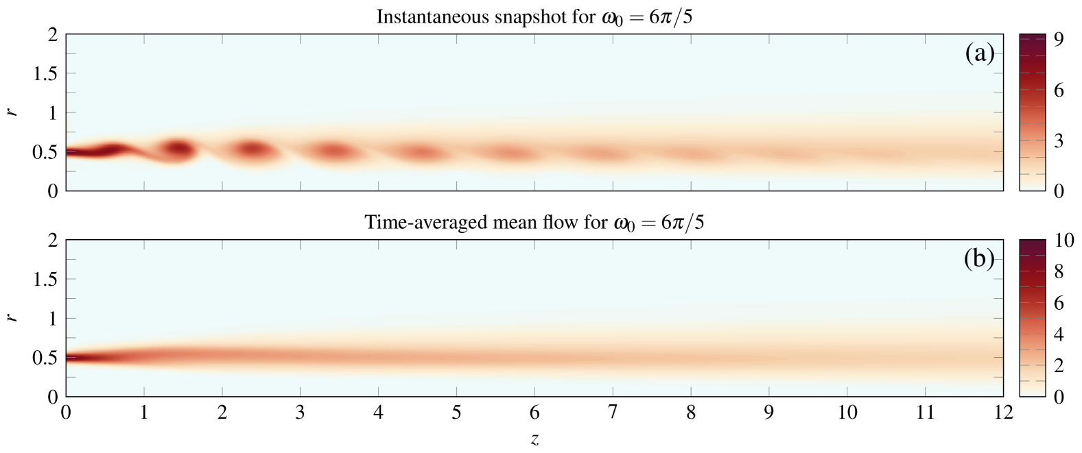
Figure 1: (a) Snapshots of the azimuthal vorticity magnitude from the $T_{0}$-periodic base flow solution $\mathbf{Q}\left(t\right)$ for a Reynolds number $Re=1000$, $S=1$ and $M=0.1$. (b) Time-averaged azimuthal vorticity magnitude from the corresponding mean state $\overline{\mathbf{Q}}$.

Once the initial transient is exhausted and the periodic state is established, we evaluate the periodic state $\mathbf{Q}\left(t_{k}\right)$ at $2\mathrm{N}_{\mathrm{h}}+1$ discrete Fourier collocation points in time defined by $t_{k}=k\Delta t$ with $\Delta t=\left(2\pi/\omega_{0}\right)/\left(2\mathrm{N}_{\mathrm{h}}+1\right)$. The mean flow is then computed by time-averaging over the sampled snapshots as

$$\overline{\mathbf{Q}}=\frac{1}{2\mathrm{N}_{\mathrm{h}}+1}\sum_{k=0}^{2\mathrm{N}_{\mathrm{h}}}\mathbf{Q}\left(t_{k}\right).$$ (30)

In this specific case, we have used $\mathrm{N}_{\mathrm{h}}=16$ which corresponds to 33 time snapshots. A snapshot of the azimuthal vorticity magnitude from the $T_{0}$-periodic base flow solution $\mathbf{Q}\left(t\right)$ is shown in figure 1(a), with its associated mean state $\overline{\mathbf{Q}}$ illustrated in figure 1(b).

4.3 Resolvent analysis about the mean flow

We first perform the resolvent analysis about the mean flow, for which a convergence test on the grid refinement is carried out and outlined in Appendix A. In the BROADCAST code (Poulain et al., 2023a), linearisation of the governing equations (27a)-(27e) about a given reference state is performed with Algorithmic Differentiation (AD) (Hascoet & Pascual, 2013). The Jacobian operator about the mean flow is computed accordingly, and the resolvent analysis about the mean flow is then performed in the frequency domain as described in §2.3.
To be consistent with Padovan & Rowley (2022), we only consider external forcing to the momentum equations and restrict the analysis to flow structures over the subdomain $\left\{\left(r,z\right)|~0\leq r\leq 2.5,0\leq z\leq 20\right\}$; this is accounted for in the definition of the space prolongation operator $\mathsfbi{B}$, which is equal to the identity for the selected state components (radial and axial momentums) within the specified domain and zero otherwise. We also restrict the output to the same state component and spatial subdomain by appositely defining the restriction operator $\mathsfbi{C}=\mathsfbi{B}^{T}$. The resulting eigenvalue problem reduces to (11); in this problem, the selected measures to evaluate the amplitude of the response and the forcing are taken to be the same and to correspond to (twice) the input-output kinetic energy estimated over the restricted domain, so that $\mathsfbi{M}_{y}=\mathsfbi{M}_{f}=\mathsfbi{M}$ and the output norm $||\hat{\boldsymbol{\phi}}||^{2}=\hat{\boldsymbol{\phi}}^{H}\mathsfbi{M}\hat{\boldsymbol{\phi}}=\int_{0}^{2.5}\int_{0}^{20}\left(\left(\rho u_{r}\right)^{2}+\left(\rho u_{z}\right)^{2}\right)\,r\text{d}r\text{dz}$. Note that $\rho\approx 1$ because of the weak compressibility and the chosen temperature ratio $S=1$. Similarly, for the input we have $||\hat{\boldsymbol{\psi}}||^{2}=\hat{\boldsymbol{\psi}}^{H}\mathsfbi{M}\hat{\boldsymbol{\psi}}$.
The harmonic gain curve outputted by this procedure is reported in figure 2 as white circles, which, in agreement with Padovan & Rowley (2022) shows a clear sub-harmonic amplification; this is explained by the sensitivity of the flow to undergo vortex pairing.

4.4 Mean resolvent analysis

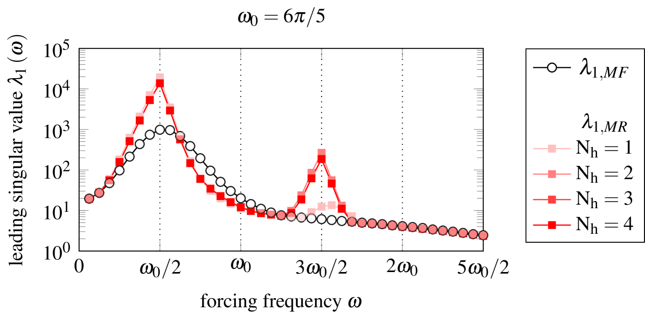
Figure 2: Leading singular value $\lambda_{1}\left(\omega\right)$, as a function of the forcing frequency $\omega$, for the periodically forced axisymmetric jet discussed in §4, which is oscillating at $\omega_{0}=6\pi/5$. Black line plus white circles: resolvent analysis about the mean flow. Red filled squares: mean resolvent analysis computed for $\mathrm{N}_{\mathrm{h}}=1,2,3$ and $4$. A good convergence is achieved already for $\mathrm{N}_{\mathrm{h}}=2$. A mesh of size $N_{r}\times N_{z}=200\times 300$ was used for this calculation.

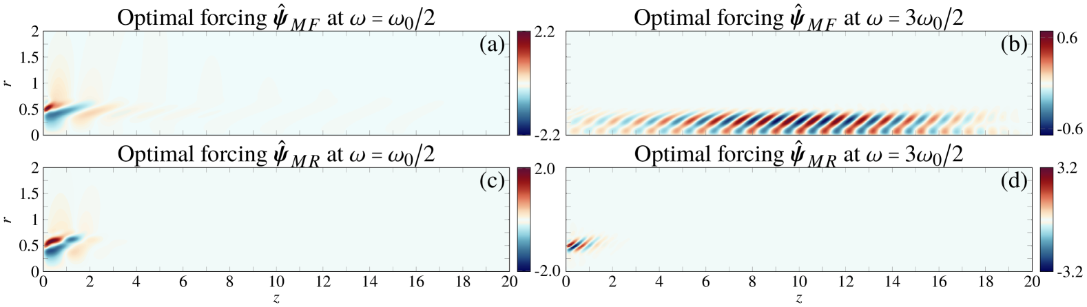
Figure 3: Real part of the axial velocity component associated with the optimal forcing mode, $\hat{\boldsymbol{\psi}}$, computed according to (a,b) the resolvent analysis about the mean flow and (c,d) the mean resolvent analysis at (a)-(c) $\omega=\omega_{0}/2$ and (b)-(d) $\omega=3\omega_{0}/2$. To ease the visual comparison, each mode has been renormalised such that its phase at a coordinate $\left(r,z\right)=\left(0.5,0.1\right)$ is zero.

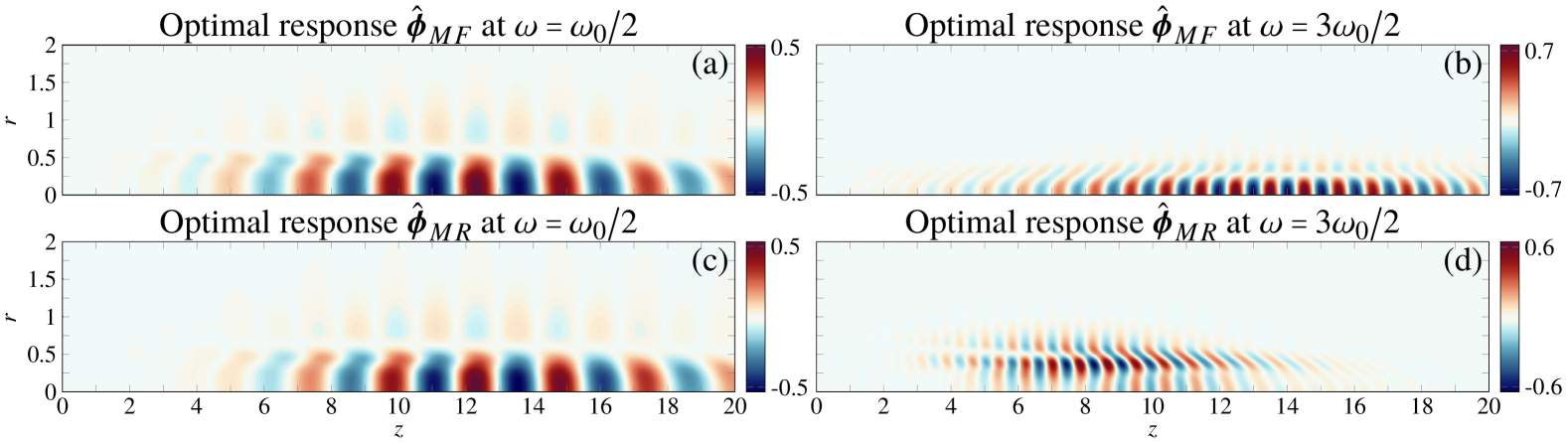
Figure 4: Real part of the axial velocity component associated with the optimal response mode, $\hat{\boldsymbol{\phi}}$, rescaled by the corresponding gain and computed according to (a,b) the resolvent analysis about the mean flow and (c,d) the mean resolvent analysis at (a)-(c) $\omega=\omega_{0}/2$ and (b)-(d) $\omega=3\omega_{0}/2$. To ease the visual comparison, each mode has been normalised such that its phase at a coordinate $\left(r,z\right)=\left(0.5,10\right)$ is zero.

While the Jacobian operator about the mean is readily obtained by linearising about the time-averaged solution $\overline{\mathbf{Q}}$, performing mean resolvent analysis requires first the extraction of the Fourier components of the unsteady Jacobian. With the aid of Algorithmic Differentiation (AD) available in BROADCAST, $2\mathrm{N}_{\mathrm{h}}+1$ instantaneous Jacobian operators, evaluated at collocation points, are computed by linearising about $\mathbf{Q}\left(t_{k}\right)$; successively, the Fourier components $\hat{\mathsfbi{J}}_{n}$ are computed by applying a Discrete Fourier Transform (DFT)

$$\hat{\mathsfbi{J}}_{n}=\frac{1}{2\mathrm{N}_{\mathrm{h}}+1}\sum_{k=0}^{2\mathrm{N}_{\mathrm{h}}}e^{-\frac{\mathrm{i}2\pi kn}{2\mathrm{N}_{\mathrm{h}}+1}}\mathsfbi{J}\left(t_{k}\right),$$ (31)

with $n\in\left[-\mathrm{N}_{\mathrm{h}},+\mathrm{N}_{\mathrm{h}}\right]$ and $k\in\left[0,2\mathrm{N}_{\mathrm{h}}\right]$. For simplicity, we will assume in the rest of the manuscript the same truncation number $\mathrm{N}_{\mathrm{h}}$ for both base flow and perturbation.
The computational approach described in §2.3 is employed here to perform, in the frequency domain, the mean resolvent analysis of the same jet configuration (see also Appendix A). The resulting leading singular value is shown in figure 2 (red markers) and compared with the analogous curve from the mean flow analysis. A convergence test regarding the number of Fourier components retained shows that a fairly good convergence is achieved already for $\mathrm{N}_{\mathrm{h}}=2$. Similarly to the harmonic resolvent analysis discussed in Padovan & Rowley (2022) (see also Appendix A), the mean resolvent predicts a much stronger amplification of sub-harmonic disturbances at $\omega\approx\omega_{0}/2$, which stems from the interactions of the perturbation with the unsteady part of the base flow overlooked by the mean flow analysis. A well-defined secondary peak is also visible at $\omega\approx 3\omega_{0}/2$; for larger frequencies the gain curve collapses on that predicted by the mean flow analysis, suggesting that the base flow unsteadiness is relatively weak, i.e. only the interactions of the external forcing with the temporal mean, and those between the external forcing and the first two harmonics of the periodic base flow are significant.
The optimal forcing modes computed at the two peak frequencies $\omega=\omega_{0}/2$ and $3\omega_{0}/2$ according to the mean flow and mean resolvent analyses are displayed in figure 3. While, at the first sub-harmonic peak, we observe mostly qualitative differences in the predicted structures from the mean flow analysis (panel (a)) and the mean resolvent analysis (panel (c)), the discrepancies are quantitatively significant at the second sub-harmonic peak, at which the two optimal forcing mode do not share at all the same spatial support, with the one from the mean resolvent mostly localised upstream near the inlet. Analogous observations can be drawn for the optimal response modes of figure 4.

$\omega$	$\gamma_{\langle\hat{\boldsymbol{\psi}}_{MF},\,\hat{\boldsymbol{\psi}}_{HR}\rangle}$	$\gamma_{\langle\hat{\boldsymbol{\psi}}_{MF},\,\hat{\boldsymbol{\psi}}_{MR}\rangle}$	$\gamma_{\langle\hat{\boldsymbol{\phi}}_{MF},\,\hat{\boldsymbol{\phi}}_{HR}\rangle}$	$\gamma_{\langle\hat{\boldsymbol{\phi}}_{MF},\,\hat{\boldsymbol{\phi}}_{MR}\rangle}$
$\omega_{0}/2$	0.8494	0.8501	0.9933	0.9934
$3\omega_{0}/2$	0.0088	0.0103	0.0731	0.0732

Table 1: Alignment coefficients, defined by (32), quantifying the relative alignment among optimal input-output structures predicted by the two resolvent analyses.

We can better quantify the relative difference of these structures by computing the alignment coefficient $0\leq\gamma\leq 1$,

$$\gamma=\frac{|\langle\mathbf{a},\mathbf{b}\rangle|}{||\mathbf{a}||\cdot||\mathbf{b}||}=\frac{|\mathbf{a}^{H}\mathsfbi{M}\mathbf{b}|}{\left(\mathbf{a}^{H}\mathsfbi{M}\mathbf{a}\right)^{1/2}\left(\mathbf{b}^{H}\mathsfbi{M}\mathbf{b}\right)^{1/2}},$$ (32)

with $\mathbf{a}$ and $\mathbf{b}$ two generic complex-valued vector fields. The values associated with these scalar products for both input and output modes are given in table 1. At $\omega=\omega_{0}/2$, the qualitative difference between the optimal response fields associated with the mean-field and mean resolvent analysis is quantified by an alignment coefficient of approximately $0.85$, while it drastically deteriorates at $\omega=3\omega_{0}/2$.

5 Projected mean resolvent modes: results and comparison

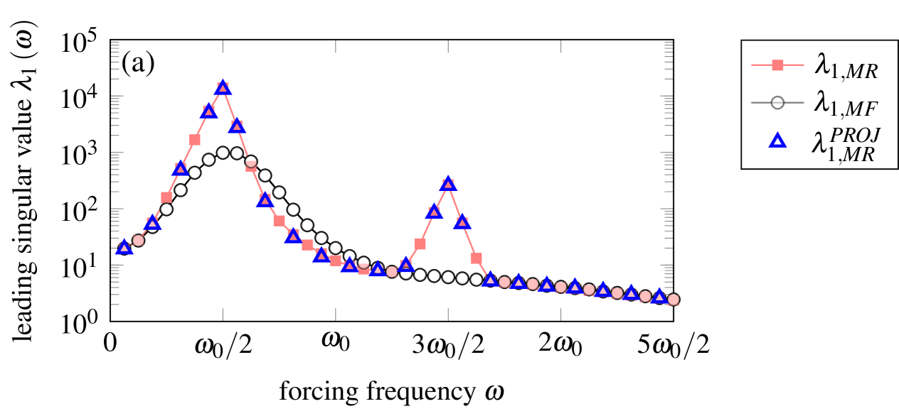
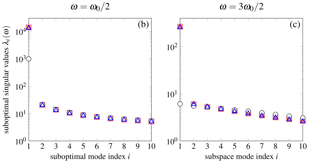
Figure 5: (a) Leading singular value $\lambda_{1}\left(\omega\right)$, as a function of the forcing frequency $\omega$, for the periodically forced axisymmetric jet discussed in §4 with $\omega_{0}=6\pi/5$. Black line plus white circles: resolvent analysis about the mean flow. Red filled squares: mean resolvent analysis computed for $\mathrm{N}_{\mathrm{h}}=2$ as in figure 2. Blue empty triangles: optimal gain predicted by the projection method discussed in §3 using a subspace of $d=60$ optimal forcing mode from the resolvent analysis about the mean flow; convergence analysis shows that a smaller subspace dimension, i.e. $d\lesssim 20$ (or even less depending on the frequency), already provides a fairly good approximation (see figure 6). (b) First 10 suboptimal singular values $\lambda_{i}\left(\omega\right)$ associated with the three analyses of panel (a) for $\omega=\omega_{0}/2$. (c) Same as in (b) but for $\omega=3\omega_{0}/2$.

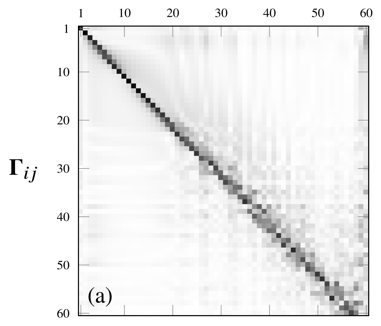
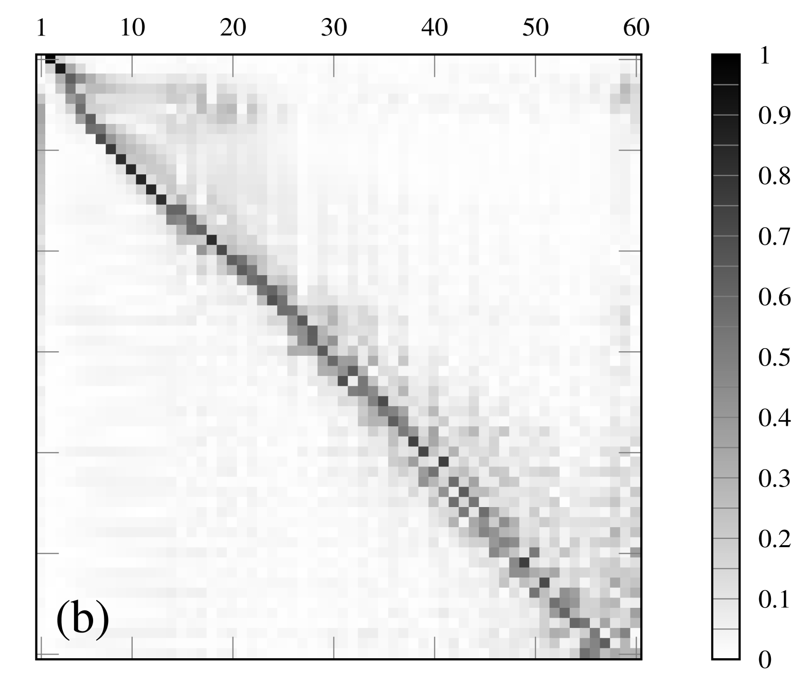
Figure 6: Matrix of projection coefficients $\boldsymbol{\Gamma}$ computed by solving (23) for (a) $\omega=\omega_{0}/2$ and (b) $\omega=3\omega_{0}/2$. The unitary norm $j$th column contains the $d$ coefficients multiplying the $d$ mean flow forcing modes to obtain, as a linear combination of these modes, the $j$th mean resolvent forcing mode.

Figure 7: Convergence of the leading singular value computed via the projection method for (a) $\omega=\omega_{0}/2$ and (b) $\omega=3\omega_{0}/2$. The values are rescaled by true value from the reference framework of §4, which is $13925.4$ in (a) and $264.7$ in (b). The lowest vertical axis limit has been selected to indicate the optimal gain from the corresponding mean flow analysis, which is $982.3$ in (a) and $6.1$ in (b). For $\omega=\omega_{0}/2$, the value of $\lambda^{PROJ}_{1,\,MR}$ obtained with a single-mode ($d=1$) is $11845.9$ (approximately $85$% of $\lambda_{1,\,MR}$), while a value of $13071.7$ is obtained for $d=60$ ($94$% of $\lambda_{1,\,MR}$). Analogously, for $\omega=3\omega_{0}/2$, we have $6.5$ for $d=1$ (approximately $2.4$% of $\lambda_{1,\,MR}$) and $257.18$ for $d=60$ ($97$% of $\lambda_{1,\,MR}$).

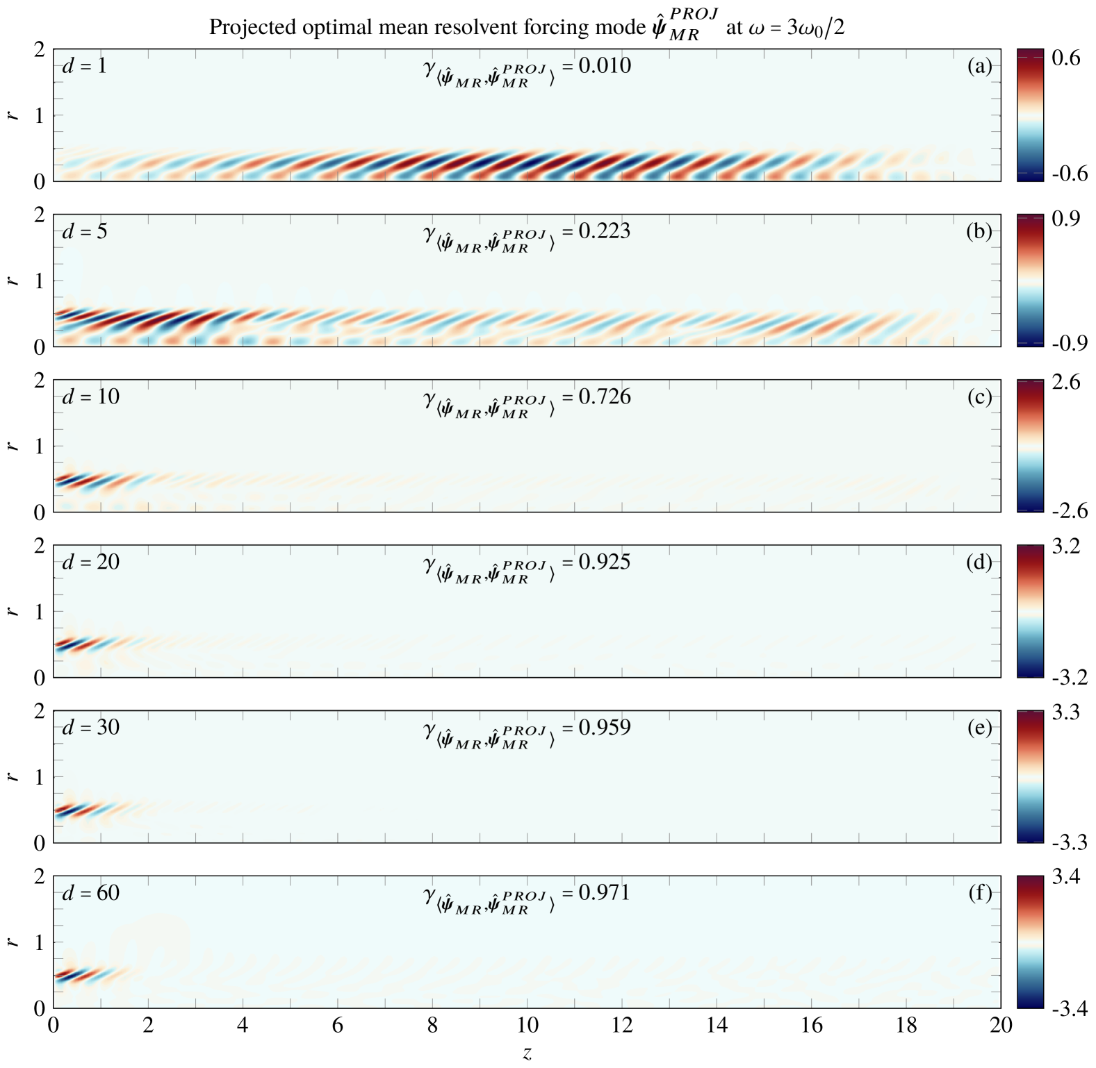
Figure 8: Real part of the axial velocity component associated with the approximated mean resolvent optimal forcing mode, $\hat{\boldsymbol{\psi}}$, computed according to the projection method using increasing subspace dimensions $d$: (a) 1, (b) 5, (c) 10, (d) 20, (e) 30 and (f) 60. To ease the visual comparison, each mode has been renormalised such that its phase at a coordinate $\left(r,z\right)=\left(0.5,0.1\right)$ is zero. We also give the value of the alignment coefficients $\gamma$ between the reference case $\hat{\boldsymbol{\psi}}_{MR}$ (not shown here) and the approximated one, with the latter reconstructed as the linear combination $\hat{\boldsymbol{\psi}}^{PROJ}_{MR}=\sum_{i=1}^{d}\hat{\mathbf{f}}^{\left(i\right)}_{0}\boldsymbol{\Gamma}_{i1}$.

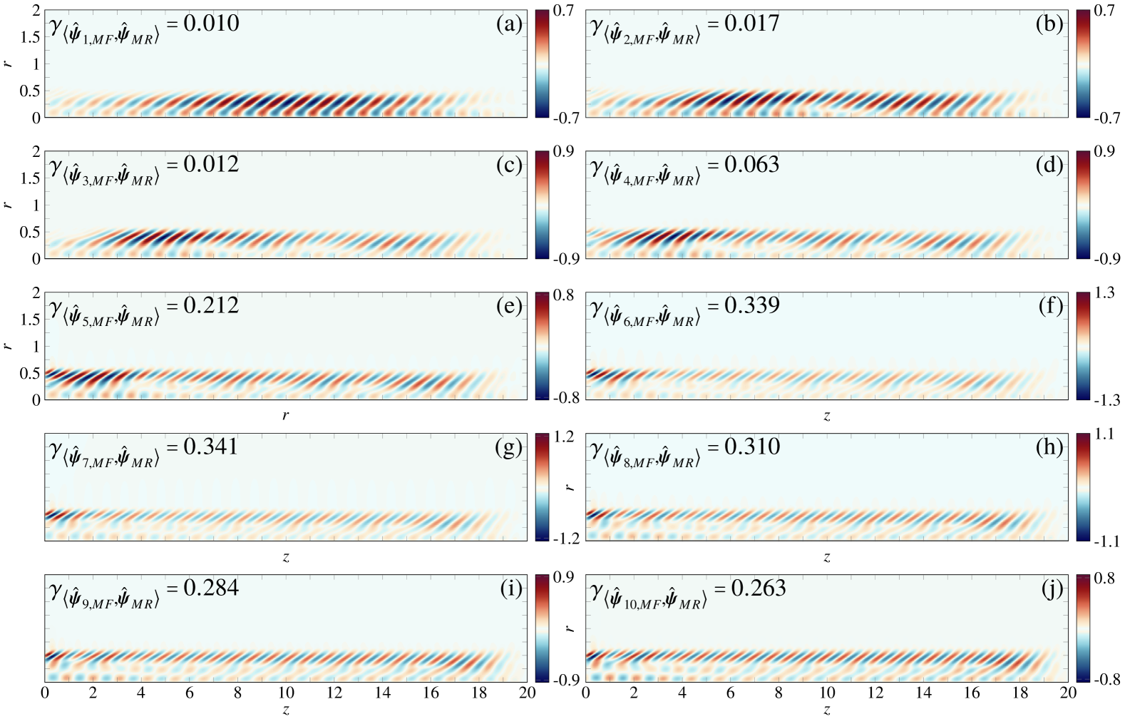
Figure 9: Real part of the axial velocity component associated with the first ten suboptimal input modes calculated according to the resolvent analysis about the mean flow, $\hat{\boldsymbol{\psi}}_{MF}$. These modes were computed for a forcing frequency $\omega=3\omega_{0}/2$, i.e. at the second subharmonic peak, as in figure 8. Each mode has been renormalised such that its phase at a coordinate $\left(r,z\right)=\left(0.5,0.1\right)$ is zero. The corresponding singular values are those shown in panel (c) of figure 5 as black circles (mean flow). The coefficients $\gamma$ given inside the left panels quantify the alignments (computed according to (32) ) between the $i$th suboptimal mean flow mode and the optimal mean resolvent mode of figure 3(d).

In this section, we demonstrate the predictive power of the projected mean resolvent analysis by applying to the same jet configuration discussed so far, for which our numerical tools have been validated against Padovan & Rowley (2022) in Appendix A.
The mean resolvent leading singular value obtained via the projection method by solving (23) is shown in figure 5(a) for different forcing frequencies (empty blue triangles). For a subspace dimension made of $d=60$ suboptimal mean flow forcing modes, we observe an excellent agreement with the results from the reference framework (filled red squares). This is not surprising at those frequencies where the predicted gain from mean resolvent and resolvent about the mean flow are close enough, e.g. at $\omega\gtrsim 2\omega_{0}$, as the subspaces from the two operators are nearly perfectly aligned. In the following, we will therefore comment mainly on the results at the two sub-harmonic peaks, $\omega=\omega_{0}/2$ and $\omega=3\omega_{0}/2$, where the largest discrepancy between $\mathsfbi{R}_{\overline{\mathbf{Q}}}$ and $\mathsfbi{R}_{0}$ is found.
At the first frequency peak, the high sensitivity of the system to sub-harmonic disturbances makes it low-rank; this is captured by both analyses, even though the optimal gain from $\mathsfbi{R}_{\overline{\mathbf{Q}}}$, which overlooks interactions with the unsteady part of the base flow, is much lower than that from $\mathsfbi{R}_{0}$. Despite some qualitative differences, figure 3 shows that approximately the same spatial support characterises the optimal forcing mode from the mean resolvent and mean flow analysis, thus, using a subspace of mean flow input mode to build the vector basis and perform the projection seems indeed a suitable choice. The matrix of projection coefficients $\boldsymbol{\Gamma}_{ij}$, where each $j$th column is an eigenvector solution of (23), shows a clear diagonal structure for a subspace dimension $d\lesssim 30$, after which the projection starts to deteriorate and spread over the off-diagonal coefficient, hence slowing down the convergence of the series.
Interestingly, at $\omega=\omega_{0}/2$, a single-mode projection ($d=1$), for which $\hat{\boldsymbol{\psi}}=\hat{\mathbf{f}}^{(1)}_{0}$ and $\boldsymbol{\Gamma}_{11}=1$, is already sufficient to significantly improve the gain prediction associated with the optimal response mode (see figures 5(b) and 7(a)). This is explainable by noticing that, even though the input is the same, interactions with the unsteady part of the flow are inherently captured by the mean resolvent operator and intrinsically manifest in the database of computed responses $\hat{\mathsfbi{Y}}$ used to construct the reduced problem (23)-(24).
The most interesting scenario here is that associated with the second frequency peak. In contradistinction to the previous case, the mean flow analysis completely overlooks the second sub-harmonic peak since the latter is purely produced by interactions with the unsteady part of the flow; this specific configuration offers a challenging test case to verify the applicability and predictive power of the projection method, as one could anticipate that the mean flow subspace can provide only a poor approximation of the actual mean resolvent modes. This is reflected in figure 5(c), where, for the mean resolvent, the large energy gap between the leading singular value and the suboptimal ones is a symptom of a low-rank behaviour; on the contrary, there is no energy gap between modes in the mean flow analysis. Yet, the projection method based on mean flow input modes predicts very well the value of the optimal gain (see blue markers in figure 5(a)).
The corresponding matrix of projection coefficients and the convergence of the leading singular value with the subspace dimension are shown, respectively, in figures 6(b) and 7(b). The projection matrix does not show a perfectly diagonal structure, and, particularly, we note how the projection of the subspace modes into the leading mean resolvent forcing mode ($\boldsymbol{\Gamma}_{i1}$, the first column in figure 6(b)) is spread over a certain amount of mean flow modes, i.e. between 10 and 20 and remains very poor for $d<5$. This is also visible in figure 7(b), showing that the value of $\lambda^{PROJ}_{1,MR}$ ramps up starting from a subspace dimension $d\approx 5$, after which it rapidly converges to the desired true value. The approximated mean resolvent optimal forcing mode is shown in figure 8, which visualises how the input energy progressively moves and localises upstream near the inlet as we increase the subspace dimension. Comparing the spatial support of the input mode in panel (a) that in panel (f) gives an intuitive explanation of how the projection is initially poor. The inspection of the spatial structures for suboptimal mean flow modes, shown in figure 9, clarifies why the convergence of $\lambda^{PROJ}_{1,MR}\left(3\omega_{0}/2\right)$ reported in figure 7(b) begins improving for subspace dimensions $d\gtrsim 5$; indeed, the spatial support of suboptimal mean flow modes progressively shifts upstream, hence favouring the projection and approximation of the leading mean resolvent mode $\hat{\boldsymbol{\psi}}_{MR}$, which is localised in the vicinity of the inlet (see figure 3(d)) .
Concerning the singular values associated with these suboptimal modes, panels (b), for $\omega=\omega_{0}/2$, and (c), for $\omega=3\omega_{0}/2$, of figure 5 show that the resolvent analysis about the mean flow predicts values of gain (black circles) similar to those computed from the mean resolvent analysis (red squares), especially for $\omega=\omega_{0}/2$; differences are, however, appreciable for $\omega=3\omega_{0}/2$, whereas the projection method provides a perfect collapse of the first ten approximated singular values (blue triangles) on the corresponding reference ones (red squares).

6 Vortex-paired configuration: effect of the base flow unsteadiness and cross-validation via time-marching

The flow configuration examined in §4 and §5 offered a test case to discuss new results on mean resolvent analysis, for which the developed algorithms and associated numerical tools could be, at least partially, validated against Padovan & Rowley (2022) (see Appendix A for details). In particular, we have briefly commented on the high sensitivity of the periodic base flow to subharmonic disturbances leading to vortex pairing (Shaabani-Ardali et al., 2019; Padovan & Rowley, 2022). Such sensitivity is qualitatively captured by the resolvent analysis about the mean flow and is mainly attributable to interactions of the subharmonic perturbation with the mean flow itself, even though interactions with the unsteady part of the periodic base flow are not negligible. Indeed, these interactions lead to quantitative differences in the optimal gain curve predicted by the mean resolvent analysis, which shows a much steeper increase in the magnitude of the singular value for sub-harmonic forcing frequencies. While discussing the convergence of the results, we have also shown that, in that particular case, two Fourier components were sufficient to represent the oscillatory base flow and describe the input-output dynamics. Moreover, the singular value curve associated with the mean resolvent analysis collapses on that of the resolvent about the mean flow already for perturbation frequencies $\omega\gtrsim 2\omega_{0}$; those two aspects combined suggest that the considered base flow is intrinsically weakly unsteady (Leclercq & Sipp, 2023), which explains why the resolvent analysis about the mean flow is sufficient to provide qualitatively good predictions, at least of the dominant subharmonic peak (yet, note that the analysis completely overlooks the second peak).
In this last section, we investigate the same type of periodic base flow, but forced at half the frequency, i.e. $\omega_{0}=3\pi/5$ instead of $\omega_{0}=6\pi/5$. Such a configuration, illustrated in figure 10, differs from the first one (see figure 10(a,b)) for the size of the coherent structures and wavelength between two consecutive vortices, which, consistently with the imposed subharmonic forcing, appears as approximately twice that of the first jet (vortex-paired configuration) (see figure 10(c,d)). We anticipate that this strongly unsteady second case represents an example for which the standard resolvent analysis about the mean flow constitutes an unsatisfactory approximation of the mean transfer function, while the latter remains generally valid, although it has to be kept in mind that the more unsteady the flow the more uncertain any LTI model become.

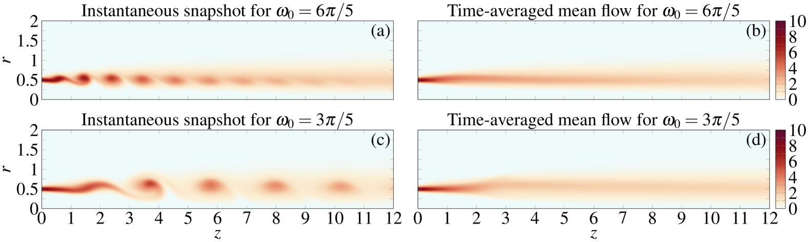
Figure 10: (a)-(c) Snapshots of the azimuthal vorticity magnitude from the $T_{0}$-periodic base flow solution $\mathbf{Q}\left(t\right)$ for (a) $\omega_{0}=6\pi/5$ and (c) $\omega_{0}=3\pi/5$. (b)-(d) Time-averaged azimuthal vorticity magnitude from the corresponding mean state $\overline{\mathbf{Q}}$ computed at (b) $\omega_{0}=6\pi/5$ and (d) $\omega_{0}=3\pi/5$. The non-dimensional parameters of interest are set to $Re=1000$ and $S=1$. The same mesh and domain size were employed in both computations.

As in §4, we perform the mean resolvent analysis and check the convergence with the number of Fourier components retained for base flow and perturbation; this is done in figure 11. In contrast to the case of §4, the present base flow requires a larger truncation number $\mathrm{N}_{\mathrm{h}}$, i.e. $\mathrm{N}_{\mathrm{h}}\gtrsim 5$ to ensure convergence, thus implying that unsteady effects are here more important. Therefore, one could anticipate that, due to stronger interactions between the perturbation and the oscillatory part of the base flow, the relative difference between the predictions from the resolvent analysis about the mean flow and mean resolvent will be greater in this scenario.

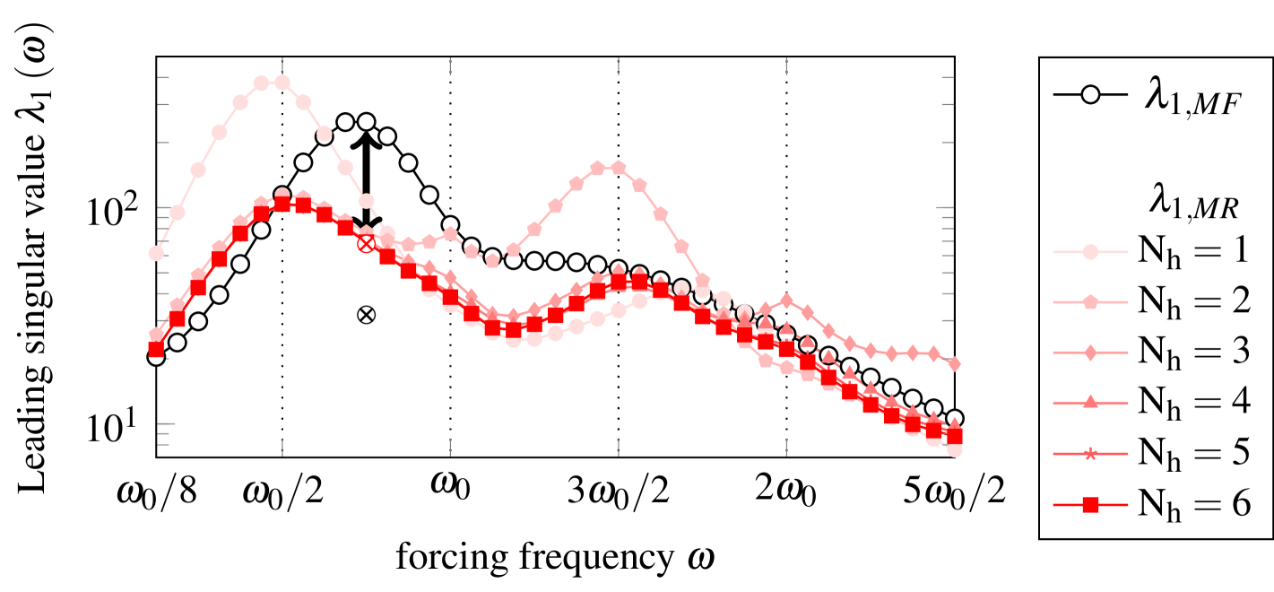
Figure 11: Leading singular value $\lambda_{1}\left(\omega\right)$, as a function of the forcing frequency $\omega$, as computed from the mean-flow analysis (black line plus white circles) mean resolvent analysis (red squares) for $\omega_{0}=3\pi/5$ and $\mathrm{N}_{\mathrm{h}}\in\left[1,6\right]$. This picture better highlights the importance of accounting for higher harmonics to guarantee convergence. We also see residual low-gain peaks at multiples of the base flow frequency $\omega_{0}$, but those peaks vanish at convergence for increasing $\mathrm{N}_{\mathrm{h}}$, i.e. $N_{h}\gtrsim 5$ (note the limit-cycle is not self-sustained here). A large energy gap, indicated by the black double-headed arrow, is observed around $\omega\approx 1.41$ between the gain prediction from mean resolvent and resolvent about the mean flow; the two red and black crosses correspond to the validation tests are be outlined in §6.1 via time-marching of the linearised equation, which confirm the mean resolvent curve (red cross) as the true optimal gain curve.

This is indeed confirmed by the inspection of the different curves displayed in figure 11. This time, the two analyses are not only quantitatively but also qualitatively different. The mean flow analysis predicts a dominant peak occurring at a frequency somewhere in the range $\omega_{0}/2\leq\omega\leq\omega_{0}$ (with $\omega_{0}=3\pi/5$), a value that is hardly linkable to any physical explanation; on the other hand, the mean resolvent analysis, predicts a maximum amplification for a subharmonic input, which is physically linkable by the system’s sensitivity to undergo further vortex-pairing; on a side comment, the gain values are here much lower than the previous case, denoting a weaker sensitivity to subharmonic amplification, i.e. to induce vortex pairing, one must now provide greater input energy.
These differences can be explained by the stronger unsteadiness of the underlying base flow, a condition under which the resolvent operator about the mean flow represents a poorer approximation of the mean resolvent operator (Leclercq & Sipp, 2023).

6.1 Validation by time-marching the forced linearised governing equations

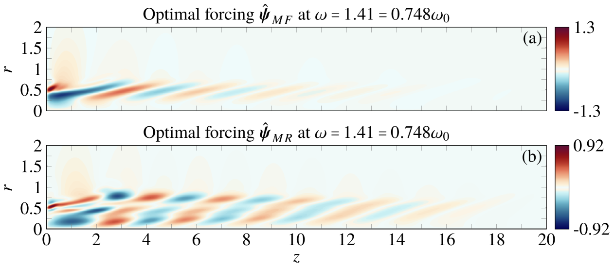
Figure 12: Real part of the axial velocity component associated with the optimal forcing mode, $\hat{\boldsymbol{\psi}}$, computed according to (a) the resolvent analysis about the mean flow and (b) the mean resolvent analysis at $\omega=1.41$. Their alignement amounts to $\gamma_{\langle\hat{\boldsymbol{\psi}}_{MF},\hat{\boldsymbol{\psi}}_{MR}\rangle}=0.69$.

For this base flow configuration, we do not have a prior reference for validation. Alternatively, we propose to perform two numerical experiments based on the time-marching of the linearised forced equation (4); these tests will also help us elucidating the time-domain version of the input projection method. We select a forcing frequency $\omega=1.41$ for which we observe the largest energy gap in the predicted harmonic gain curve from the mean resolvent and resolvent about the mean flow (see black arrow in figure 11; in one case, the structure of the external harmonic forcing is taken to be the optimal forcing outputted from the mean flow analysis, while in the second case we take the optimal forcing from the mean resolvent analysis.
Before moving forward, let us comment on these two forcing structures, which are illustrated in figure 12. As in the case of figure 3 in §4, both structures showed in panels (a) and (b) are tilted against the shear; this is consistent with the Orr mechanism (W. M. Orr, 1907), according to which the perturbation energy may grow transiently in time, as the perturbation field, initially inclined against the shear, is gradually rotated by the shear associated with the base or mean flow. The mean resolvent input structure of figure 3(c) showed the spatial support localised slightly more upstream than its mean flow counterpart (see figure 3(a)), and it was characterised by two lobes in the radial direction. On the contrary, the support of the mean resolvent mode of figure 12(b) is more extended downstream than the corresponding mean flow mode (see figure 12(a)), and it has three radial lobes, with an alignment $\gamma$ between the two fields approximately equal to 0.69. A precise explanation for the latter structure remains to be elucidated and is beyond the scope of the present paper.
Equation (4) is integrated in time using Algorithmic Differentiation (AD) in BROADCAST, with only the linearised residual vector that is computed at each time step; in such a way, we avoid going through the tedious harmonic resolvent formalisms in the frequency domain, and the connection with the harmonic transfer operator does not need to be explicitly invoked.
Three time-signals associated with the post-transient state of the linear response probed at three different downstream locations and the corresponding Power Spectral Density (PSD) are shown, respectively, in figures 13 and 14. In these figures, the red lines indicate the outputs obtained by forcing with the optimal mean resolvent input mode, whereas the black dashed lines are obtained by forcing with the optimal input mode from the resolvent about the mean flow. The PSD spectra show multiple frequency peaks relevant to the dynamics and centred at the expected frequencies according to the formula (25). An on-the-fly harmonic average is implemented, as explained in §3.2, to extract, among these peaks, the one oscillating at the input frequency $\omega$, which represents the mean (phase-averaged) response, hence avoiding the storage of $\mathbf{y}^{\prime}\left(t\right)$.

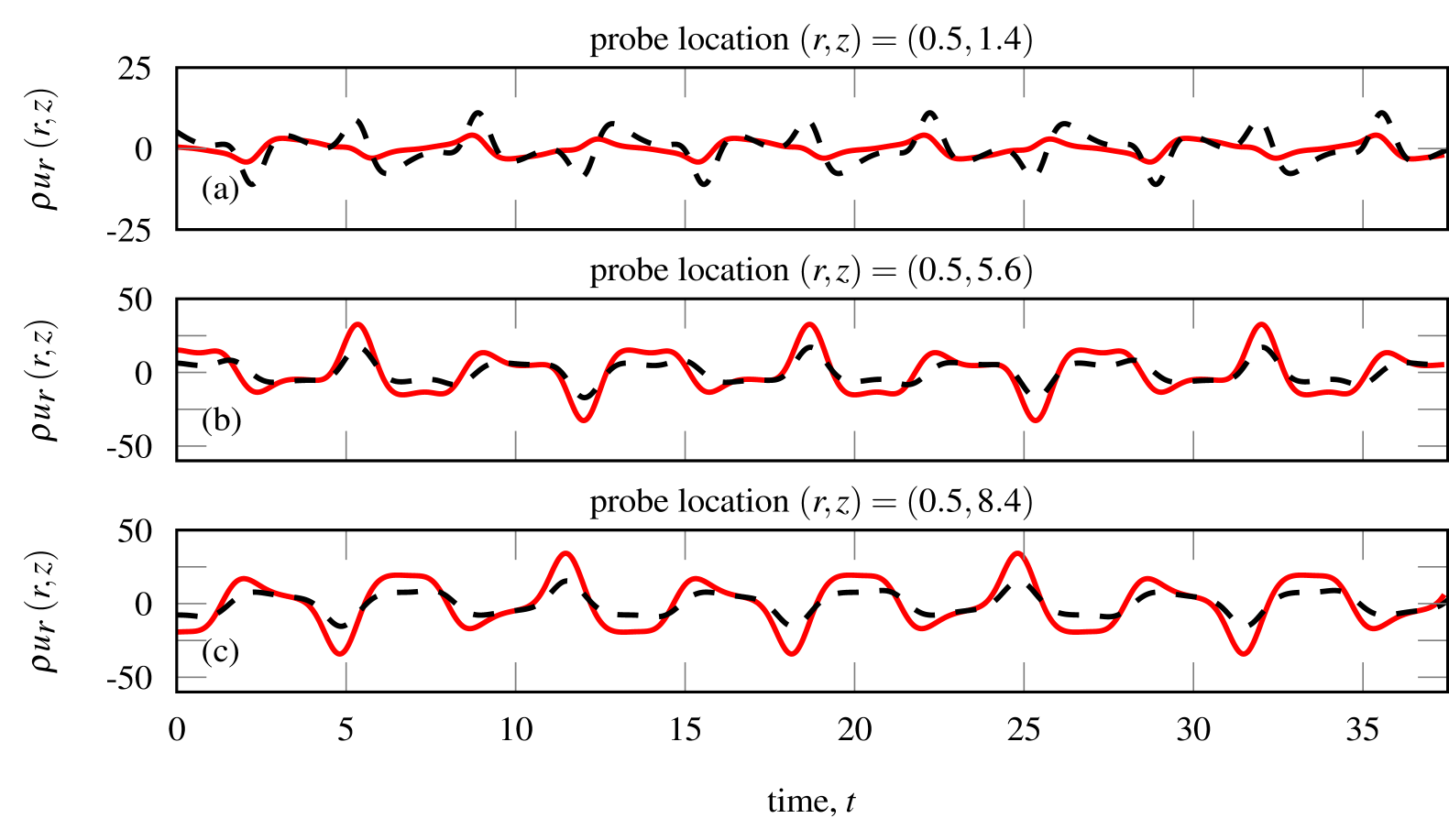
Figure 13: Three time-signals associated with the post-transient state of the linear response probed at three different downstream locations. Black dashed line: linear response to the optimal input mode from the resolvent about the mean flow. Red line: linear response to the optimal mean resolvent input mode.

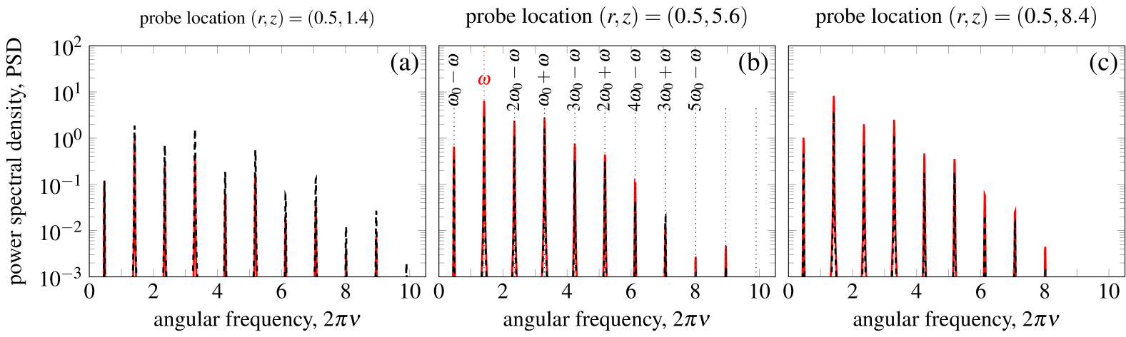
Figure 14: Power Spectral Density (PSD) associated with the three probes of figure 13 and computed using the built-in Matlab function fft with Hann windowing. Black dashed line: linear response to the optimal input mode from the resolvent about the mean flow. Red line: linear response to the optimal mean resolvent input mode.

The norm of the Fourier component of the extracted response eventually gives the value of the gain, to be compared with that reported in figure 11. If the mean resolvent analysis previously performed in the frequency domain (red curve in figure 11 is correct, the structure of the external forcing selected for this numerical experiment is already optimal, and the associated gain should collapse on the red curve of figure 11. On the contrary, the input mode from the resolvent about the mean flow can only be suboptimal for the actual linearised system, so that the associated gain should lie below the red curve for the same forcing frequency. The red and black crosses reported in figure 11 show that this is indeed the case, hence cross-validating the implementation of the mean resolvent analysis in both time and frequency domains.
If this time-based procedure is repeated by taking as inputs a sufficient number of suboptimal input modes from the mean-flow resolvent, i.e. $\hat{\mathbf{f}}_{0}^{\left(i\right)}$, the resulting mean responses $\hat{\mathbf{y}}_{0}^{\left(i\right)}$ can be gathered in $\hat{\mathsfbi{Y}}$ and the projection method applied as described in §3, one obtains an approximation of the mean resolvent optimal modes and gains, provided that the dimension of the subspace $d$ is sufficiently large.
Importantly, the investigation of the vortex-paired configuration discussed in this section represents an example of an unsteady base flow, for which the standard resolvent analysis about the mean flow constitutes an unsatisfactory approximation of the mean transfer function (Leclercq & Sipp, 2023).

7 Conclusions

Starting from the definition of the mean transfer function introduced by Leclercq & Sipp (2023), we have begun this manuscript by providing a rigorous framework to compute input-output mean resolvent modes of periodic flows. This was done by drawing a connection between the mean transfer function and the harmonic transfer function when considering linear time-periodic system (LTP) subjected to exponentially modulated periodic (EMP) input signals (Wereley & Hall, 1990, 1991; Padovan et al., 2020; Padovan & Rowley, 2022). Specifically, we have reformulated the mean resolvent operator in terms of a harmonic resolvent operator, where instead of maximising the overall energy of the response, one maximises the mean (phase-averaged) response to an external time-harmonic forcing oscillating at frequency $\omega$.
By considering an incompressible axisymmetric laminar jet periodically forced at the inlet with different angular frequencies $\omega_{0}$, we have shown that the standard resolvent analysis about the mean flow is wrong by an order of magnitude on the amplitude of the receptivity peak for the case with $\omega_{0}/2$. In some other configurations, the frequency of the subharmonic receptivity mechanism is completely off; this is, e.g., the case of base flow oscillating at $\omega_{0}=3\pi/5$, where there is a 50% error on the predicted frequency peak. In addition, the mean resolvent captures a peak in receptivity at $3\omega_{0}/2$ that is completely absent from the classical resolvent analysis and that stems from interactions between the external perturbation and the unsteady part of the base flow, which are overlooked by the mean-field analysis; at this secondary peak, the mean resolvent optimal forcing mode is located far upstream in the shear layer, whereas the mean-field analysis predicts a mode with the support spread far downstream.
Successively, using such a framework as a reference case for validation, we have developed an alternative methodology to approximate optimal forcing and response modes of the mean resolvent operator. The method, which we refer to as the projection method, uses a vector subspace of suboptimal input modes from the resolvent operator about the mean flow to approximate mean resolvent modes. We have shown how to formulate and apply the method in both the frequency and time-domain, with the resulting predictions that have been shown in excellent agreement with the validated reference case.
The generalization of the projection method to stochastic, chaotic and turbulent flows, where dynamic linearity does not hold (i.e. ensemble-averaging is necessary even if for harmonic inputs) is currently under investigation and will be reported elsewhere. The final target is the application of a time-domain version of the method to stochastic and turbulent flows, for which mean resolvent analysis could be compared with popular mean-flow resolvent analysis.

Appendix A Validation of the numerical tools

The present Appendix is devoted to the validation of the numerical tools employed in this study to produce the results presented throughout the manuscript. This is done taking as test case the first jet configuration oscillating at $\omega_{0}=6\pi/5$, for which a direct comparison with Padovan & Rowley (2022) (P&R) is possible.

A.1 Grid convergence for mean-flow analysis

Concerning the mean-flow analysis, in figure 15(a), we report the leading singular value $\lambda_{1,MF}\left(\omega\right)$ as a function of the forcing frequency $\omega$ and computed for four different grids as explained in §2.3. Results are robust and agree fairly well with the reference case from P&R (black solid line). The dependence on the mesh refinement is mostly visible at higher frequencies, with a grid $\mathrm{N}_{\mathrm{r}}\times\mathrm{N}_{\mathrm{z}}=200\times 300$ ($\mathrm{N}=4\times\mathrm{N}_{\mathrm{r}}\times\mathrm{N}_{\mathrm{z}}=240\,000$) that provides a satisfactory trade-off. We notice how, even for the finest mesh, the present results do not perfectly overlap with the reference case; such discrepancy could be caused by the weak compressibility effects allowed for in our formulation, although a more likely explanation could reside in the fact that Padovan & Rowley (2022) used a third-order upwind scheme to discretise the advective term, whereas we used a fifth-order scheme (see the comparison between Bugeat et al. (2019) and Poulain et al. (2023a) on the strong effect of the scheme order on the convergence of results). Nevertheless, the discrepancy is mostly visible at frequencies characterised by a relatively low gain when compared to the predicted dominant peak found at $\omega\approx\omega_{0}/2$.

A.2 GMRES solver with block-Jacobi preconditioner for harmonic resolvent analysis

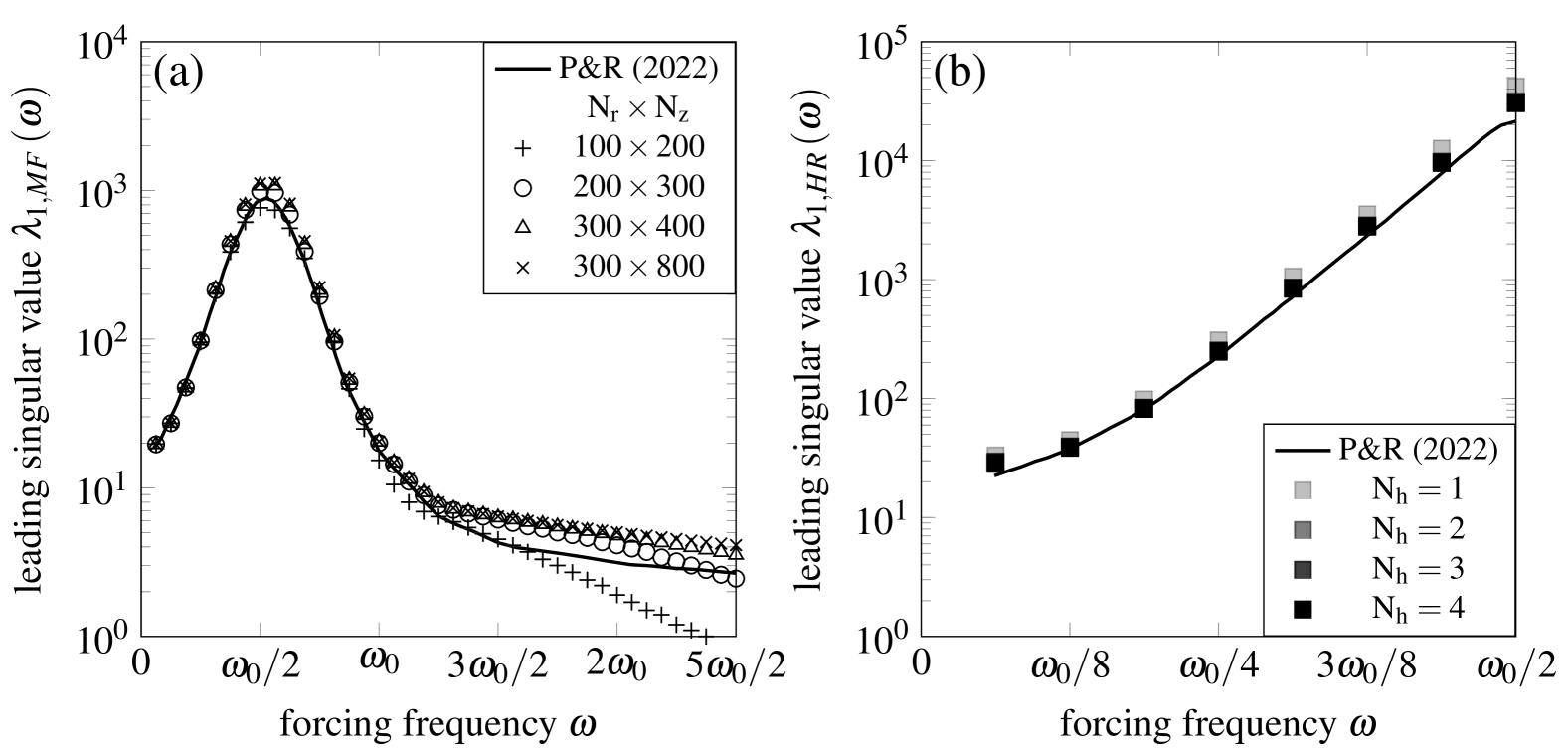
Figure 15: (a) Leading singular value $\lambda_{1,MF}\left(\omega\right)$ predicted by the resolvent analysis about the mean flow for the axisymmetric jet forced by an axial inflow velocity oscillating periodically described at $\omega_{0}=6\pi/5$ (§4). The Reynolds number is $Re=1000$. The analysis is performed on an interval of forcing frequency $\omega$ ranging from $0.1$ to $5/2$ times the base flow frequency. The black solid line corresponds to the mean flow analysis of Padovan & Rowley (2022) (P&R). Markers correspond instead to the present results obtained for four different grid refinements. The finest mesh is the same as P&R. (b) Harmonic resolvent leading singular value $\lambda_{1,HR}\left(\omega\right)$ as computed by P&R for $Re=1000$ (black solid line) and from the present analysis (markers) for $\mathrm{N}_{\mathrm{h}}=1,2,3$ and $4$ over the relevant set of frequencies $0\leq\omega\leq\omega_{0}/2$, with $\omega_{0}=6\pi/5$. A good convergence is achieved already for $\mathrm{N}_{\mathrm{h}}=2$ (the data for $\mathrm{N}_{\mathrm{h}}=3$ and $4$ are indistinguishable from those for $\mathrm{N}_{\mathrm{h}}=2$). For this computation, a mesh of size $200\times 300$ were used.

As commented in §2.3, in this study, mean resolvent analysis has been computed in the frequency domain using an iterative solver based on Generalised Minimal Residual (GMRES) algorithms (Rigas et al., 2021; Poulain et al., 2024a) with a block-Jacobi preconditioner, which is efficient for diagonally-dominant matrices, i.e. for weakly unsteady flows. The code was also made parallel and distributed using PETSc, with each processor core handling a $\left(\mathrm{M}\times\mathrm{M}\right)$-block, corresponding to a single Fourier component, for which a sparse direct LU method was applied using the external package MUMPS (Amestoy et al., 2000).
From our best knowledge, no previous computation of mean resolvent modes have been reported yet in the literature, hence making a direct validation impossible. Nevertheless, these tools have been designed based on the close connection drawn between the mean resolvent and the harmonic transfer operator for LTP systems. As such, the tools are readily applicable to perform harmonic resolvent analysis, for which validation against Padovan & Rowley (2022) is instead possible.
To do so, we consider the more general EMP input $\hat{\boldsymbol{\mathsfbi{\mathcal{F}}}}=\left\{\ldots,\hat{\mathbf{f}}_{-1}^{T},\hat{\mathbf{f}}^{T}_{0},\hat{\mathbf{f}}_{+1}^{T},\ldots\right\}^{T}$$\in\mathbb{C}^{\left(\mathrm{N}\times\left(2\mathrm{N}_{\mathrm{h}}+1\right)\right)\times 1}$ (i.e. the restriction operators $\boldsymbol{\mathcal{P}}_{y}$ and $\boldsymbol{\mathcal{P}}_{f}$ in §2.2.2 are taken to be the identity $\boldsymbol{\mathcal{I}}$). The most energetic input-output dynamics maximising the energy gain over the whole forcing vector $\hat{\boldsymbol{\mathsfbi{\mathcal{F}}}}_{HR}\neq\mathbf{0}$, i.e. $\lambda_{HR}^{2}=||\hat{\boldsymbol{\mathsfbi{\mathcal{Y}}}}_{HR}^{opt}||^{2}/||\hat{\boldsymbol{\mathsfbi{\mathcal{F}}}}_{HR}^{opt}||^{2}=||\hat{\boldsymbol{\Phi}}_{HR}||^{2}/||\hat{\boldsymbol{\Psi}}_{HR}||^{2}$, is now computed by solving the very large eigenvalue problem

$$\left(\boldsymbol{\mathsfbi{\mathcal{R}}}^{H}\boldsymbol{\mathsfbi{\mathcal{M}}}_{y}\boldsymbol{\mathsfbi{\mathcal{R}}}\right)\hat{\boldsymbol{\Psi}}_{j,HR}=\lambda_{j,HR}^{2}\boldsymbol{\mathsfbi{\mathcal{M}}}_{f}\hat{\boldsymbol{\Psi}}_{j,HR},$$ (33)

which is formally equivalent to that presented in Padovan & Rowley (2022), with $\boldsymbol{\mathsfbi{\mathcal{M}}}_{y}$ and $\boldsymbol{\mathsfbi{\mathcal{M}}}_{f}$ block-diagonal matrices formed from $\mathsfbi{M}_{y}\in\mathbb{R}^{\mathrm{K}\times\mathrm{K}}$ and $\mathsfbi{M}_{f}\in\mathbb{R}^{\mathrm{M}\times\mathrm{M}}$, respectively. The associated response is obtained as $\hat{\boldsymbol{\Phi}}_{j,HR}=\boldsymbol{\mathsfbi{\mathcal{R}}}\hat{\boldsymbol{\Psi}}_{j,HR}$.
The procedure discussed above is validated against the predictions from Padovan & Rowley (2022), which are reported in figure 15(b). The number of harmonics retained is progressively increased from $\mathrm{N}_{\mathrm{h}}=1$ to $\mathrm{N}_{\mathrm{h}}=4$. We observe that $\mathrm{N}_{\mathrm{h}}=2$ is already sufficient to ensure a fair convergence and a good agreement with the reference case. Note that, for the harmonic resolvent analysis, both the perturbation $\tilde{\mathbf{q}}\left(t\right)$ and its measure $\tilde{\mathbf{y}}\left(t\right)$ in (6a)-(6b) are fully determined by its Fourier coefficients over the set of forcing frequency $0\leq\omega\leq\omega_{0}$, which is why the curve is not reported elsewhere (see Padovan & Rowley (2022)).
As expected, while the peak in the mean flow analysis is the signature of strong interaction between forcing and mean flow, the much larger gain predicted by the harmonic resolvent shows that interactions with the unsteady part of the base flow also contribute to the input-output subharmonic dynamics.

Acknowledgements

The authors acknowledge Dr Samir Beneddine for the fruitful insights about the numerical implementation of the parallelised GMRES solver in PETSc/SLEPc.
The authors also acknowledge Dr Javier Sierra-Ausín for the stimulating discussion on the linear response theory and its connection with the mean linear response to forcing of dynamical systems about an attractor.

Declaration of Interests

The authors report no conflict of interest.

References

- Amestoy et al. (2000) Amestoy, P. R., Duff, I. S., L’Excellent, J.-Y. & Koster, J. 2000 Mumps: a general purpose distributed memory sparse solver. In International Workshop on Applied Parallel Computing, pp. 121–130. Springer.
- Audiffred et al. (2024) Audiffred, D. B. S., Cavalieri, A. V. G., Maia, I. A., Martini, E. & Jordan, P. 2024 Reactive experimental control of turbulent jets. J. Fluid Mech. 994, A15.
- Balay et al. (et al. 2019) Balay, S., Abhyankar, S., Adams, M., Brown, J., Brune, P., Buschelman, K., Dalcin, L., Dener, A., Eijkhout, V. & Gropp, W. et al. 2019 PETSc Users Manual. Argonne National Laboratory.
- Beneddine et al. (2016) Beneddine, S., Sipp, D., Arnault, A., Dandois, J. & Lesshafft, L. 2016 Conditions for validity of mean flow stability analysis. J. Fluid Mech. 798, 485–504.
- Bugeat et al. (2019) Bugeat, B., Chassaing, J.-C., Robinet, J.-C. & Sagaut, P. 2019 3d global optimal forcing and response of the supersonic boundary layer. J. Comp. Physics 398, 108888.
- Cabell et al. (2006) Cabell, R. H., Kegerise, M. A., Cox, D. E. & Gibbs, G. P. 2006 Experimental feedback control of flow-induced cavity tones. AIAA Journal 44 (8), 1807–1816.
- Carini & Quadrio (2010) Carini, M. & Quadrio, M. 2010 Direct-numerical-simulation-based measurement of the mean impulse response of homogeneous isotropic turbulence. Phys. Rev. E 82 (6), 066301.
- Cattafesta et al. (1999) Cattafesta, L., Shukla, D., Garg, S. & Ross, J. 1999 Development of an adaptive weapons-bay suppression system. In 5th AIAA/CEAS Aeroacoustics Conference and Exhibit, p. 1901.
- Cinnella & Content (2016) Cinnella, P. & Content, C. 2016 High-order implicit residual smoothing time scheme for direct and large eddy simulations of compressible flows. J. Comp. Phys. 326, 1–29.
- Dahan et al. (2012) Dahan, J. A., Morgans, A. S. & Lardeau, S. 2012 Feedback control for form-drag reduction on a bluff body with a blunt trailing edge. J. Fluid Mech. 704, 360–387.
- Dergham et al. (2011) Dergham, G., Sipp, D. & Robinet, J.-C. 2011 Accurate low dimensional models for deterministic fluid systems driven by uncertain forcing. Phys. Fluids 23 (9).
- Farghadan et al. (2024) Farghadan, A., Jung, J., Bhagwat, R. & Towne, A. 2024 Efficient harmonic resolvent analysis via time stepping. Theor. Comp. Fluid Dyn. pp. 1–23.
- Franceschini et al. (2022) Franceschini, L., Sipp, D., Marquet, O., Moulin, J. & Dandois, J. 2022 Identification and reconstruction of high-frequency fluctuations evolving on a low-frequency periodic limit cycle: application to turbulent cylinder flow. J. Fluid Mech. 942, A28.
- Garnaud et al. (2013) Garnaud, X., Lesshafft, L., Schmid, P. J. & Huerre, P. 2013 The preferred mode of incompressible jets: linear frequency response analysis. J. Fluid Mech. 716, 189–202.
- Hascoet & Pascual (2013) Hascoet, L. & Pascual, V. 2013 The tapenade automatic differentiation tool: principles, model, and specification. ACM Trans. Math. Softw. (TOMS) 39 (3), 1–43.
- Hwang & Cossu (2010a) Hwang, Y. & Cossu, C. 2010a Amplification of coherent streaks in the turbulent couette flow: an input–output analysis at low reynolds number. J. Fluid Mech. 643, 333–348.
- Hwang & Cossu (2010b) Hwang, Y. & Cossu, C. 2010b Linear non-normal energy amplification of harmonic and stochastic forcing in the turbulent channel flow. J. Fluid Mech. 664, 51–73.
- Islam & Sun (2024) Islam, M. R. & Sun, Y. 2024 Identification of cross-frequency interactions in compressible cavity flow using harmonic resolvent analysis. J. Fluid Mech. 1000, A13.
- Karban et al. (2020) Karban, U., Bugeat, B., Martini, E., Towne, A., Cavalieri, A. V. G., Lesshafft, L., Agarwal, A., Jordan, P. & Colonius, T. 2020 Ambiguity in mean-flow-based linear analysis. J. Fluid Mech. 900, R5.
- Kegerise et al. (2002) Kegerise, M., Cattafesta, L. & Ha, C.-S. 2002 Adaptive identification and control of flow-induced cavity oscillations. In 1st Flow Control Conference, p. 3158.
- Kestens & Nicoud (1998) Kestens, T. & Nicoud, F. 1998 Active control of an unsteady flow over a rectangular cavity. In 4th AIAA/CEAS Aeroacoustics Conference, p. 2348.
- Kook et al. (2002) Kook, H., Mongeau, L. & Franchek, M. A. 2002 Active control of pressure fluctuations due to flow over helmholtz resonators. J. Sound Vib. 255 (1), 61–76.
- Lazarus & Thomas (2010) Lazarus, A. & Thomas, O. 2010 A harmonic-based method for computing the stability of periodic solutions of dynamical systems. Comptes Rendus Mécanique 338 (9), 510–517.
- Leclercq & Sipp (2023) Leclercq, C. & Sipp, D. 2023 Mean resolvent operator of a statistically steady flow. J. Fluid Mech. 968, A13.
- Lesshafft et al. (2006) Lesshafft, L., Huerre, P., Sagaut, P. & Terracol, M. 2006 Nonlinear global modes in hot jets. J. Fluid Mech. 554, 393–409.
- Luchini et al. (2006) Luchini, P., Quadrio, M. & Zuccher, S. 2006 The phase-locked mean impulse response of a turbulent channel flow. Phys. Fluids 18 (12).
- Maia et al. (2021) Maia, I. A., Jordan, P., Cavalieri, A. V. G., Martini, E., Sasaki, K. & Silvestre, F. 2021 Real-time reactive control of stochastic disturbances in forced turbulent jets. Phys. Rev. Fluids 6 (12), 123901.
- Marconi et al. (2008) Marconi, U. M. B., Puglisi, A., Rondoni, L. & Vulpiani, A. 2008 Fluctuation–dissipation: response theory in statistical physics. Phys. Reports 461 (4-6), 111–195.
- Martinelli et al. (2009) Martinelli, F., Quadrio, M. & Luchini, P. 2009 Turbulent drag reduction by feedback: a wiener-filtering approach. In Advances in Turbulence XII: Proceedings of the 12th EUROMECH European Turbulence Conference, September 7–10, 2009, Marburg, Germany, pp. 241–246. Springer.
- Martini et al. (2021) Martini, E., Rodríguez, D., Towne, A. & Cavalieri, A. V. G. 2021 Efficient computation of global resolvent modes. J. Fluid Mech. 919, A3.
- Matsumoto et al. (2021) Matsumoto, T., Otsuki, M., Ooshida, T. & Goto, S. 2021 Correlation function and linear response function of homogeneous isotropic turbulence in the eulerian and lagrangian coordinates. J. Fluid Mech. 919, A9.
- McKeon & Sharma (2010) McKeon, B. J. & Sharma, A. S. 2010 A critical-layer framework for turbulent pipe flow. J. Fluid Mech. 658, 336–382.
- Mongeau et al. (1998) Mongeau, L., Kook, H. & Franchek, M. A. 1998 Active control of flow-induced cavity resonance. In 4th AIAA/CEAS Aeroacoustics Conference, p. 2349.
- Monokrousos et al. (2010) Monokrousos, A., Åkervik, E., Brandt, L. & Henningson, D. S. 2010 Global three-dimensional optimal disturbances in the blasius boundary-layer flow using time-steppers. J. Fluid Mech. 650, 181–214.
- Morra et al. (2019) Morra, P., Semeraro, O., Henningson, D. S. & Cossu, C. 2019 On the relevance of reynolds stresses in resolvent analyses of turbulent wall-bounded flows. J. Fluid Mech. 867, 969–984.
- Padovan et al. (2020) Padovan, A., Otto, S. E. & Rowley, C. W. 2020 Analysis of amplification mechanisms and cross-frequency interactions in nonlinear flows via the harmonic resolvent. J. Fluid Mech. 900, A14.
- Padovan & Rowley (2022) Padovan, A. & Rowley, C. W. 2022 Analysis of the dynamics of subharmonic flow structures via the harmonic resolvent: Application to vortex pairing in an axisymmetric jet. Phys. Rev. Fluids 7 (7), 073903.
- Pickering et al. (2021) Pickering, E., Rigas, G., Schmidt, O. T., Sipp, D. & Colonius, T. 2021 Optimal eddy viscosity for resolvent-based models of coherent structures in turbulent jets. J. Fluid Mech. 917, A29.
- Poulain et al. (2024a) Poulain, A., Content, C., Schioppa, A., Nibourel, P., Rigas, G. & Sipp, D. 2024a Adjoint-based optimisation of time-and span-periodic flow fields with space–time spectral method: Application to non-linear instabilities in compressible boundary layer flows. Comp. & Fluids 282, 106386.
- Poulain et al. (2024b) Poulain, A., Content, C., Schioppa, A., Nibourel, P., Rigas, G. & Sipp, D. 2024b Adjoint-based optimisation of time-and span-periodic flow fields with space-time spectral method: Application to non-linear instabilities in compressible boundary layer flows. Comp. & Fluids 282, 106386.
- Poulain et al. (2023a) Poulain, A., Content, C., Sipp, D., Rigas, G. & Garnier, E. 2023a Broadcast: A high-order compressible cfd toolbox for stability and sensitivity using algorithmic differentiation. Comput. Phys. Commun. 283, 108557.
- Poulain et al. (2023b) Poulain, A., Content, C., Sipp, D., Rigas, G. & Garnier, E. 2023b Optimal location for steady wall blowing or heating actuators in a hypersonic boundary layer. In AERO 2023-57th 3AF International Conference on Applied Aerodynamics.
- Rathnasingham & Breuer (2003) Rathnasingham, R. & Breuer, K. S. 2003 Active control of turbulent boundary layers. J. Fluid Mech. 495, 209–233.
- Rigas et al. (2021) Rigas, G., Sipp, D. & Colonius, T. 2021 Nonlinear input/output analysis: application to boundary layer transition. J. Fluid Mech. 911, A15.
- Ruelle (2009) Ruelle, D. 2009 A review of linear response theory for general differentiable dynamical systems. Nonlinearity 22 (4), 855.
- Russo & Luchini (2016) Russo, S. & Luchini, P. 2016 The linear response of turbulent flow to a volume force: comparison between eddy-viscosity model and dns. J. Fluid Mech 790, 104–127.
- Savarino et al. (2024) Savarino, F., Poulain, A., Sipp, D. & Rigas, G. 2024 Optimal transitional mechanisms in oblique shock wave-boundary layer interaction using non-linear input/output analysis. In AIAA SCITECH 2024 Forum, p. 2552.
- Sciacovelli et al. (2021) Sciacovelli, L., Passiatore, D., Cinnella, P. & Pascazio, G. 2021 Assessment of a high-order shock-capturing central-difference scheme for hypersonic turbulent flow simulations. Comp. & Fluids 230, 105134.