A Practically Scalable Approach to the Closest Vector Problem
for Sieving via QAOA with Fixed Angles

Abstract

The NP-hardness of the closest vector problem (CVP) is an important basis for quantum-secure cryptography, in much the same way that integer factorisation’s conjectured hardness is at the foundation of cryptosystems like RSA. Recent work with heuristic quantum algorithms [1] indicates the possibility to find close approximations to (constrained) CVP instances that could be incorporated within fast sieving approaches for factorisation. This work explores both the practicality and scalability of the proposed heuristic approach to explore the potential for a quantum advantage for approximate CVP, without regard for the subsequent factoring claims. We also extend the proposal to include an antecedent “pre-training” scheme to find and fix a set of parameters that generalise well to increasingly large lattices, which both optimises the scalability of the algorithm, and permits direct numerical analyses. Our results further indicate a noteworthy quantum speed-up for lattice problems obeying a certain ‘prime’ structure, approaching fifth order advantage for QAOA of fixed depth $p=10$ compared to classical brute-force, motivating renewed discussions about the necessary lattice dimensions for quantum-secure cryptosystems in the near-term.

I Introduction

The conjectured hardness of integer (prime) factorisation makes it a central problem to modern information security, becoming the foundation for many widespread public-key cryptosystems, such as RSA [2]. No classical algorithm has yet been found – nor do we ever expect to find one – for factoring in polynomial time (see e.g. Zhang et al. [3]).

However, it is well known that these cryptosystems are vulnerable to quantum adversaries, following Peter Shor’s seminal paper uncovering that fault-tolerant quantum computation allows one to factor composite integers in polynomial-time [4]. Since its proposal, we have seen many successful experimental demonstrations of Shor’s algorithm on trivial problem instances [5, 6, 7, 8].

There have been many new proposals for cryptosystems based on different problems that are believed to be secure against any adversary with a large, fault-tolerant quantum computer (see Bernstein and Lange [9] for a recent review). Most attention is given to lattice-based cryptography [10, 11, 12, 13, 14, 15, 16]. Whilst there has been no shortage of counter-arguments against some of these works [17, 18, 19, 20, 21, 22], proposals based on lattices offer arguably the most promising route to quantum-secure cryptosystems. This is reinforced by the fact that three of the four standardised postquantum secure cryptosystems by NIST are based on lattices (see section 2.3 of Alagic et al. [23], or the NIST website [24]).

I.1 Quantum-accelerated Sieving on a Lattice

Classical factoring algorithms often use a method called sieving to find smooth relation pairs (sr-pairs; a.k.a. fac-relations). Most famously, the quadratic sieve [25, 26] and the general number sieve [27, 28] (and their variants) are the fastest known classical algorithms at time of writing (see Boudot et al. [29]). In these algorithms, sieving is a major bottleneck; e.g. the factoring record set for RSA-250 in 2020 required a computational cost of some 2,700 core years, roughly 90.7% of which is accounted for by the sieving procedure [29]. It is thus very motivating to find a fast approach to the search for sr-pairs – the faster we find them, the faster we factor.

Claus Peter Schnorr has presented a number of theoretical works for lattice-based sieving methods for integer factorisation [30, 31, 32]. Recently, Yan et al. [1] proposed to accelerate Schnorr’s lattice sieving by way of nearest neighbour search via the quantum approximate optimisation algorithm (QAOA) [33].

The principle claim advertised by these works is that this method reduces the spatial requirements for factoring an integer $N$ to $O(\log N/\log\log N)$ qubits. Many have presented strong evidence that this is a considerable underestimate [34, 35, 36, 37], and relies on outdated assumptions in the underlying theoretical framework of Schnorr [32]. Moreover, we note the omission of any time-complexity analysis, and thus a disregard for a consideration of the practical utility of their algorithm.

Besides the contention for the suitability of a lattice-based sieving method like Schnorr’s [38, 37], the claim in Yan et al. [1] implies a potential quantum advantage for the (approximate) solving of a particular form of closest vector problem (CVP), which, if realised, has further implications for the security parameters required in lattice-based cryptosystems. We take a particular interest in the QAOA subroutine used to solve this CVP, and specifically with its practical scalability towards larger problem instances.

Furthermore, we extend the subroutine with an antecedent pre-training step for the parameters of the QAOA’s ansatz to obtain fixed angles, which allows us to greatly simplify our analyses (as in Boulebnane and Montanaro [39], and Brandao et al. [40]) and dramatically reduce the computational workload. In parallel with Prokop and Wallden [41], which performs similar analysis for the shortest vector problem (SVP), this is one of the first applications of fixed angles to a cryptographically significant problem, facilitating novel – and much neglected – analysis of time complexity.

I.2 Our Contributions

For clarity, we now outline our contributions, primarily extending from the works of Yan et al. [1] and Schnorr’s collection of works for sieving on a lattice [30, 31, 32], and from Boulebnane and Montanaro [39] and Brandao et al. [40] for QAOA with fixed angles:

• A simple yet robust pre-training scheme that dramatically reduces the computational requirements for refining solutions to the CVP.

• Novel time-complexity analysis of a QAOA-based sieving method, using our own implementation derived from Khattar and Yosri [36]. The code for our experiments can be found in [42].

• An optimal scaling for the time complexity and ‘generalisability’ of the method with respect to lattice dimension by our proposed extension. Interestingly, for fixed depth QAOA (for $p$ up to $10$), we achieve polynomial advantage compared to brute-force, that exceeds significantly the “usual” Grover-type quadratic speed-up .

In undertaking the above, we provide an empirical analysis of the prospective security of cryptosystems based on lattice problems with respect to newer variational methods, giving indication for the required security parameters (e.g. lattice dimension) within such schemes. This is important insight due to the rapidly growing interest in, and usage of, variational algorithms driven by their suitability for near-term hardware [44].

I.3 Limitations to Application and Scope

There are two major limitations that should be taken into account considering the expected impact of our results in practice, and for the scope of their utility.

Firstly, since we adopt the underlying framework from Yan et al. [1] for the sake of analysis, we inherent their search space: constant size in each basis-vector (dimension), leading to space-complexity $O(n)$ and search space of the form $2^{O(n)}$. However, for similar works with the shortest vector problem (SVP), it is well-known that a size $O(\log n)$ is required for each basis-vector, and thus a search space of $2^{O(n\log n)}$ is needed to ensure that the true Shortest Vector is within the search space [45, 46]. Consequently, we do not have guarantees that the quality of the solution is close to the true Closest Vector, asymptotically. This is also related with limitations of Schnorr’s method and with the ultimate claim of factorisation [32, 1] (see appendix B). While we are restricted in this same way, we can still say something about solution quality; namely, we can give empirical observation on the degree of improvement over the classical guarantees of Babai’s nearest plane algorithm [47].

Secondly, by motivating our CVP via a factorisation problem, we are working with a restricted structure in our lattice. As such, our work can be framed as an analysis of ‘best-case scenario’ lattice problems, wherein assumptions about the discrete gaps between basis vectors can be utilised to design an optimistic algorithm. We will show that exponential effort is required even for this constrained lattice, which can be taken as further evidence against the claims of sublinear factoring, though nonetheless imply a quantum advantage for CVP on certain lattices.

The results of this work are most appropriately interpreted as an understanding of the practical scalability of this kind of neighbourhood search on a particularly constrained lattice. These constraints allow us to leverage inherent symmetries of the problem to design a highly effective pre-training scheme. Whether this can be generalised, e.g. to arbitrary CVP structures or for tighter approximations, remains an important open question.

II Background and Preliminaries

II.1 Prime Factorisation and Sieving

This section gives an overview of the current state of classical integer factorisation. We give essential definitions in factoring and number theory, and reduce the problem of factoring to the problem of finding sr-pairs.

Definition II.1 (Integer factorisation problem)

Given an odd composite integer $N>2$, find the prime factors $p,q$ (with $p<q$) such that $N=p\cdot q$.

Let $P_{n}=\{p_{i}\}_{i=0,\dots,n}$ denote the $n$-th prime basis, where $p_{i}$ is the $i$-th prime number, and $p_{0}:=-1$ allows us the capacity to represent negative integers.

Definition II.2 (Smooth number)

An integer is called $p_{n}$-smooth if all its factors are in $P_{n}$. We call $p_{n}$ the smooth bound.

Definition II.3 (Smooth relation pair)

Moreover, a pair of $p_{n}$-smooth numbers $(u_{j},v_{j})$ are called a $p_{n}$-smooth relation pair (sr-pair; a.k.a. fac-relation in Schnorr [32]) if for $e_{i,j},e^{\prime}_{i,j}\in\mathbb{N}$, we have that

$$u_{j}=\prod_{i=1}^{n}p_{i}^{e_{i,j}}\phantom{\int}\text{and}\phantom{\int}u_{j}-v_{j}N=\prod_{i=0}^{n}p_{i}^{e_{i,j}^{\prime}}\ .$$ (1)

The method for factoring that forms the foundations for many of the most efficient classical algorithms goes back to works like Kraitchik [48] and Morrison and Brillhart [49], and was later developed by Dixon [50]. Much of this discussion comes from Schnorr [32].

Given $n+1$ sr-pairs $(u_{j},v_{j})$, and taking the quotient of the terms in eq. (1), we have for $e_{i,j},e_{i,j}^{\prime}\in\mathbb{N}$ that

$$\frac{u_{j}-v_{j}N}{u_{j}}\equiv\prod_{i=0}^{n}p_{i}^{e_{i,j}^{\prime}-e_{i,j}}\equiv 1\mod N\ ,$$ (2)

since $u_{j}-v_{j}N\equiv u_{j}\mod N$ for any $(u_{j},v_{j})$. Now, any solution $t_{1},\dots,t_{n+1}\in\{0,1\}$ of the equations

$$\sum_{j=1}^{n+1}t_{j}(e_{i,j}^{\prime}-e_{i,j})\equiv 0\mod 2\ ,$$ (3)

for $i=0,\dots,n$ solves a difference of squares $X^{2}-1=(X-1)(X+1)=0\mod N$ by

$$X=\prod_{i=0}^{n}p_{i}^{\frac{1}{2}\sum_{j=1}^{n+1}t_{j}(e_{i,j}^{\prime}-e_{i,j})}\mod N\ .$$ (4)

If $X\neq\pm 1\mod N$, then this yields two nontrivial factors $\text{gcd}(X\pm 1,N)$ of $N$, where $\text{gcd}(\cdot)$ denotes the greatest common divisor algorithm, which may be efficiently computed using Euclid’s algorithm. This idea comes from Fermat’s method for factoring.

Solutions to (3) can be obtained within $O(n^{3})$ bit operations since the dimension of the linear system is $O(n)$, and so we are free to neglect this minor part of the workload in factoring $N$. Hence, the bottleneck in factoring is in finding these $n+1$ sr-pairs.

II.2 Lattices and Lattice Problems

Definition II.4 (Euclidean Lattice)

A (Euclidean) lattice $\mathcal{L}$ is a discrete additive subgroup of $\mathbb{R}^{n}$; that is, a subset $\mathcal{L}\subseteq\mathbb{R}^{n}$ that is closed under addition and subtraction, and wherein there exists some $\varepsilon>0$ such that any two distinct lattice points $\mathbf{x}\neq\mathbf{y}\in\mathcal{L}$ are separated by a distance of a least $\|\mathbf{x}-\mathbf{y}\|\geq\varepsilon$.

For a basis matrix $B=[\mathbf{b}_{1},\dots,\mathbf{b}_{m}]\in\mathbb{R}^{n\times m}$ consisting of $m$ linearly independent column vectors in $\mathbb{R}^{n}$, the lattice $\mathcal{L}(B)=\{B\mathbf{x}:\mathbf{x}\in\mathbb{Z}^{m}\}$ is generated by all integer linear combinations of $\mathbf{b}_{1},\dots\mathbf{b}_{m}$. Intuitively, a lattice is simply a regular ordering of points.

Following these semantics, the dimension of $\mathcal{L}$ is $n$, and its rank is $m$. When $n=m$, the lattice $\mathcal{L}$ (and the matrix $B$) are called full rank.

II.2.1 Properties of lattices

There are a couple of interesting properties to notice: lattices are (1) dense; and (2) hard to approximate. For a given region, there may be many lattice points, which can make finding specific points difficult. And, given an arbitrary point, finding nearby points is again difficult.

Definition II.5 (Successive minima)

The successive minima for a lattice $\mathcal{L}\subseteq\mathbb{R}^{n}$ are the positive values $\lambda_{1}(\mathcal{L})\leq\dots\leq\lambda_{n}(\mathcal{L})$, where $\lambda_{k}(\mathcal{L})$ is the smallest radius of a zero-centred ball containing $k$ linearly independent vectors of $\mathcal{L}$.

Thus, $\lambda_{1}=\lambda_{1}(\mathcal{L})$ is the shortest nonzero vector in $\mathcal{L}$.

Definition II.6 (Hermite constant)

The minimal $\gamma$ satisfying $\lambda_{1}^{2}\leq\gamma(\det\mathcal{L})^{2/n}$ for all lattices of dimension $n$ is called the Hermite constant $\gamma_{n}$, where $\det\mathcal{L}=(\det B^{T}B)^{1/2}$ is the determinant of $\mathcal{L}$.

II.2.2 Problems on lattices

Definition II.7 (Shortest Vector Problem)

Given a basis $B$ for a lattice $\mathcal{L}(B)$, find a vector $\mathbf{v}\neq\mathbf{0}\in\mathcal{L}$ such that $\|\mathbf{v}\|=\lambda_{1}(\mathcal{L})$, where $\|\mathbf{v}\|=(\mathbf{v}^{T}\mathbf{v})^{1/2}$.

Often it suffices to be only ‘close’ to the true shortest vector $\lambda_{1}$. In these cases, we refer instead to an approximate shortest vector problem ($\alpha$-SVP) for which the condition in definition II.7 is amended as $\|\mathbf{v}\|\leq\alpha\cdot\lambda_{1}(\mathcal{L})$ for approximation factor $\alpha\geq 1$.

The exact value of $\lambda_{1}$ can, in itself, be hard to obtain due to the inherent hardness of the SVP (and of $\alpha$-SVP). It may then be preferable to instead define the problem according to a (relatively) easily computable value relating to $\lambda_{1}$. For example, we can again amend the condition in definition II.7 to $\|\mathbf{v}\|\leq r\cdot(\det\mathcal{L})^{1/n}$ to obtain the $r$-Hermite shortest vector problem ($r$-Hermite SVP). This allows us to check solutions far more easily and thus efficiently, although we lose accuracy in the comparison with the true shortest vector.

Definition II.8 (Closest Vector Problem)

Given a basis $B$ for a lattice $\mathcal{L}(B)$, and a target vector $\mathbf{t}\in\text{Span}(B)$, find a vector $\mathbf{v}\in\mathcal{L}$ such that the distance $\|\mathbf{v}-\mathbf{t}\|$ is minimised; i.e. that $\|\mathbf{v}-\mathbf{t}\|=\text{dist}(\mathcal{L},\mathbf{t})$.

Figure 1: Visualising a two-dimensional, full rank lattice $\mathcal{L}$ generated by the basis $B=[\mathbf{b_{1}},\mathbf{b_{2}}]$. Shown in red is the shortest vector $\lambda_{1}(\mathcal{L})$ solving the SVP for this lattice. Shown in blue is a CVP with target $\mathbf{t}$, solved by the lattice vector $\mathbf{v}$.

Again, there exists an approximate closest vector problem ($\alpha$-CVP) to weaken the condition of closeness in definition II.8, and the $r$-approximate closest vector problem ($r$-$Abs$CVP) weakens the condition further to bring this distance to within $r$, which could, for example, be computed according to $\det\mathcal{L}$ in place of $\text{dist}(\mathcal{L},\mathbf{t})$.

All of these problems are understood to be difficult – especially in higher dimensions – to such a degree that even a quantum advantage may be insufficient to yield a polynomial-time solution. Specifically, the decision variant of SVP (GapSVP) is conjectured to be NP-hard [51], and solving either of SVP or GapSVP within a polynomial factor requires superpolynomial time with quantum computation [52]. In general, CVP is thought to be even harder [53, 54, 55], and is known to be NP-hard [55].

For the interested reader, Micciancio and Goldwasser [55] remains a prominent text in the complexity of lattice problems for applications in cryptography.

II.3 Quantum Approximate Optimisation Algorithm

A good introduction to variational quantum algorithms in general is offered by Cerezo et al. [44]. In this work, we will focus exclusively on perhaps the most widely studied variational algorithm: quantum approximate optimisation algorithm (QAOA) due to Farhi et al. [33]. We are especially interested in the possibility of pre-training a fixed set of angles (see section II.4), for which QAOA is an ideal candidate [40].

QAOA was originally inspired by the quantum adiabatic algorithm [56, 57]. Adiabatic evolution is replaced with several rounds of propagation between a problem Hamiltonian $\hat{H}_{C}$, which encodes the solution to an optimisation problem $C(z)$ over binary variables $z=z_{1},z_{2},\dots$ within its ground state, defining the unitary operator

$$U(\gamma,\hat{H}_{C})=e^{-i\gamma\hat{H}_{C}}\ ,$$ (5)

and mixer Hamiltonian $B$, whose ground-state is known, defining the unitary operator

$$U(\beta,B)=e^{-i\pi\beta B}=\prod_{j}e^{i\pi\beta\sigma^{x}_{j}/2}\ ,$$ (6)

parameterised by angles $0\leq\gamma\leq 2\pi$ and $0\leq\beta\leq\pi$ respectively, where $\sigma^{x}_{j}$ denotes a Pauli-$X$ operator applied on the $j$-th qubit.

We open a uniform superposition over computational basis states to yield an initial state $|s\rangle=\frac{1}{\sqrt{2}}\sum_{z}|z\rangle$. Then, for some integer number of ansatz layers $p>0$, we define the angle-dependent state

$$\begin{split}|\gamma,\beta\rangle=&U(\beta_{p},B)U(\gamma_{p},\hat{H}_{C})\cdots\\ &\cdots U(\beta_{1},B)U(\gamma_{1},\hat{H}_{C})|s\rangle\ ,\end{split}$$ (7)

parameterised by angles $\gamma\equiv\gamma_{1}\dots\gamma_{p}$ and $\beta\equiv\beta_{1}\dots\beta_{p}$.

It is shown in Farhi et al. [33] that

$$\lim_{p\to\infty}\min_{\gamma,\beta}\langle\gamma,\beta|\hat{H}_{C}|\gamma,\beta\rangle=\min_{z}C(z)\ ,$$ (8)

which implies that the optimisation problem can be solved with enough repetitions, if only a good set of angles can be selected. Pessimistically, we can use an outer optimisation loop on a classical computer to search for a good set within the optimisation landscape of $C(z)$ [44]. Optimistically, there may be precedence to neglect much or all of this optimisation by fixing these angles.

II.4 Fixed Angles for QAOA

Interesting remarks have been made about the apparent independence between the optimisation landscape for the objective function (of some e.g. combinatorial search problem) and the specific problem instance [58, 59, 40].

In particular, Brandao et al. [40] fix the $\gamma$ and $\beta$ parameters to show that, when instances are generated by some reasonable distribution, the objective function is nearly independent of the chosen instance. It is suggested that this could be leveraged to find a good set of parameters for some given instance (possibly at great computational expense), which can then be utilised at no further expense for any subsequent (typical) instance. Indeed, removing the need to search for parameters in each instance allows us to neglect the outer optimisation loop once a set has been found, and hence the amortised cost tends to zero inversely with the number of instances being solved [40].

More recently, Boulebnane and Montanaro [39] have given numerical results that speak to the validity of a “fixed angle” scheme for eventually obtaining a quantum advantage with QAOA for random $k$-SAT. They find a significant improvement over Grover’s algorithm [60] with greatly reduced quantum circuit depth.

In all of these works, the method for obtaining a fixed set of angles is either to take a random (usually small) problem instance to train (e.g. in Brandao et al. [40]), or the angles may be randomised within some sensible interval. Preliminary investigation with such a scheme led to underwhelming results for this work (see appendix C), so we seek a more robust pre-training scheme that will find a good set of angles more deliberately.

III Reducing Sieving to a CVP on the Prime Lattice

The problem of finding small integers whose product is close to $N$ is translated into the equivalent problem of finding logarithms of small numbers whose sum is close to $\log N$. In doing this, we have given ourselves a combinatorial optimisation problem which may be directly expressed as a linear system of lattice vectors.

Of course, the lattice vectors in question must exhibit the properties of the logarithms of primes so that a linear combination represents an sr-pair. Schnorr [32] suggests to construct the so-called prime lattice whose basis is defined according to the corresponding factor basis. Some additional randomness is baked in to bring about unique lattice problems that (hopefully) have unique solutions. See appendix B for details concerning Schnorr’s method.

Concretely, define the prime lattice $\mathcal{L}(B_{n,c})$ by

$$B_{n,c}=\begin{pmatrix}f(1)&0&\cdots&0\\ 0&f(2)&\cdots&0\\ \vdots&\vdots&\ddots&\vdots\\ 0&0&\cdots&f(n)\\ N^{c}\ln p_{1}&N^{c}\ln p_{2}&\cdots&N^{c}\ln p_{n}\end{pmatrix}\ ,$$ (9)

with $c$ the precision parameter, and where the $f(i)$ elements correspond to elements from a random permutation of $\{\lceil 1/2\rceil,\lceil 2/2\rceil,\dots,\lceil n/2\rceil\}$. Hence, the number of lattices arising from a factor basis $P_{n}$ scales as $O(n!)$.

The target for our CVP on this lattice is defined directly from the composite integer $N$ to be factored:

$$\mathbf{t}=\begin{pmatrix}0&\stackrel{{\scriptstyle n}}{{\cdots}}&0&N^{c}\ln N\end{pmatrix}^{\top}\ .$$ (10)

III.1 Suitability of Approximation

A critical consideration of the method due to Schnorr [32] is that an approximate solution to this CVP is sufficient. Theoretical results [30, 31, 32] leave the door open to the existence of an approximate solution that improves on polynomial-time classical approximations, but which does not succumb to the NP-hardness of exactly solving the full CVP [53, 54, 55]. We draw from excellent discussion in Aboumrad et al. [35], extended from Schnorr [32], to detail the rationale behind this possibility.

Suppose we obtain a set of coefficients $e_{j}$ for the linear combination of basis vectors of the prime lattice $\mathcal{L}(B_{n,c})$ that approximately solve the CVP. That is, suppose we have found $e_{j}$ such that

$$\varepsilon:=\bigg{|}\sum_{j=1}^{n}e_{j}\ln p_{n}-\ln N\bigg{|}\approx 0\ .$$ (11)

If we set that $u=\prod_{e_{j}\geq 0}p_{j}^{e_{j}}$ and $v=\prod_{e_{j}>0}p_{j}^{-e_{j}}$, then we obtain $\ln|(\frac{u}{vN})|=\varepsilon$. By Taylor’s theorem, $u-vN=vN(e^{\varepsilon}-1)\approx\varepsilon vN$. Schnorr [32]’s argument is that since $\varepsilon$ is small, $u-vN$ is also small and thus likely to be $p_{n}$-smooth. By definition II.3, $(u,v)$ is an sr-pair.

If we are content to run multiple problem instances, then we need only find $e_{j}$ coefficients for eq. (11) that reduce $\varepsilon$ to be small enough such that the probability that they correspond to a useful sr-pair is ‘good enough’.

There are strong doubts concerning the validity of this method at scale [34, 36, 35, 37, 38], and in particular that this probability decays exponentially such that sr-pairs cannot be found by refinement alone (or, at least, not quickly enough to care). More detail is given to these concerns in appendix B.

This work does not look to affirm nor deny Schnorr’s algorithm as a method for factoring; our interest lies exclusively with the efficiency with which this CVP can be ‘refined’ by a variational approach, and thus what we might say about the quantum advantage one might find for problems on the prime lattice.

III.2 Hyperparameters

So far, we can see that the hyperparameter $n$ has the role of dictating all of: (1) the dimension of the lattice; (2) the size of the factor basis, and hence the number of integers that may be considered $p_{n}$-smooth; and (3) the number of unique prime lattices that can be constructed in our sieving procedure.

Increasing $n$ comes with a dimension-complexity trade-off: with a larger smooth bound $p_{n}$, we can more easily find smooth numbers, but we will require more of them (recall we require $n+1$ sr-pairs in section II.1). The exact correlation between $n$ and time complexity is not well understood in this context, and much of our work here is dedicated to uncovering this relationship empirically.

The $N^{c}$ term in the formulation of $B_{n,c}$ gives parameterisable precision to the lattice. This is conjectured to be positively correlated with the probability of finding solutions to problems within this lattice, though some have voiced concerns that this is unsubstantiated [36, 37]. As for our later analyses, we will fix $c$ and, similar to Yan et al. [1] and Khattar and Yosri [36], we exchange $N^{c}$ for $10^{c}$ to give a consistent basis between instances. This will improve the effectiveness of pre-training.

Refinement Performance with Increasing Lattice Dimension (by Depth $p$)

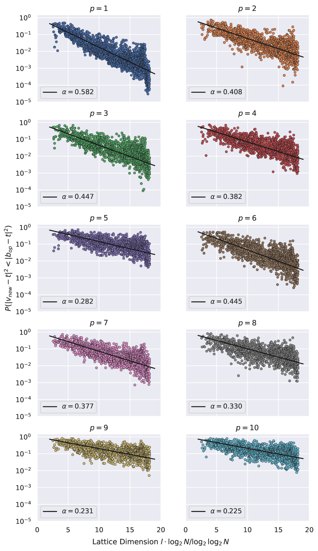
Figure 2: The probability to refine the classical solution (for cases in which a refinement exists) by exact lattice dimension for different depths $p$ of QAOA circuits. Each plot is equipped with a best-fit curve of the form $1/2^{\alpha n}$, and $\alpha$ is shown.

IV A Method for CVP Refinement

IV.1 Polynomial-time Classical Approximation

We begin by considering a polynomial-time procedure that serves up an approximate solution to the CVP. This procedure consists of a lattice reduction step using the LLL-reduction algorithm [61] (described in appendix A) followed by Babai’s nearest plane algorithm [47], which brings us to within a factor $2(2/\sqrt{3})^{n}$ of $\text{dist}(\mathcal{L},\mathbf{t})$. The following is a high-level summary of Babai’s algortihm.

Having produced an LLL-reduced basis $D=[\mathbf{d}_{1},\dots,\mathbf{d}_{n}]$ for $B_{n,c}$, we perform Gram-Schmidt orthogonalisation (without column normalisation) to yield $\tilde{D}=[\tilde{\mathbf{d}}_{1},\dots,\tilde{\mathbf{d}}_{n}]$. The nearest plane algorithm then comprises a series of projections of the target vector $\mathbf{t}$ onto $\text{Span}(\tilde{D})$ followed by a rounding of the coefficients to snap onto a nearby lattice point. Concretely, begin by setting $\mathbf{b}_{op}\leftarrow\mathbf{t}$, then for each $j$ in $n,\dots,1$ compute the Gram-Schmidt coefficient $\mu_{j}=\langle\mathbf{t},\tilde{\mathbf{d}}_{j}\rangle/\langle\tilde{\mathbf{d}}_{j},\tilde{\mathbf{d}}_{j}\rangle$, round to the nearest integer $c_{j}=\lceil\mu_{j}\rfloor$, and update $\mathbf{b}_{op}\leftarrow\mathbf{b}_{op}-c_{j}\mathbf{d}_{j}$.

Intuitively, when considering index $j$, we are taking the $j$-dimensional subspace $\text{Span}\{\tilde{\mathbf{d}}_{1},\dots,\tilde{\mathbf{d}}_{j}\}$ and finding the integer $c_{j}$ that minimises the distance from $c_{j}\mathbf{b}_{j}+\text{Span}\{\tilde{\mathbf{d}}_{1},\dots,\tilde{\mathbf{d}}_{j-1}\}$ to $\mathbf{t}$ [35]; in each step, we find the nearest (hyper)plane, giving the algorithm its name.

IV.2 Refinement as a Minimum-eigenstate Optimisation Problem

Suppose we have found an approximate solution $\mathbf{b}_{op}=\sum_{j=1}^{n}c_{j}\mathbf{d}_{j}$, where again the $c_{j}=\lceil\mu_{j}\rfloor$ are the rounded Gram-Schmidt coefficients. Our goal is to ‘refine’ this solution efficiently.

The potential for a quantum advantage falls out of the rounding operation $\lceil\cdot\rfloor$; classically, this operation considers rounding in each direction one after another (i.e. $\lceil\cdot\rceil$ and $\lfloor\cdot\rfloor$), but quanutmly they can be considered simultaneously [1]. Doing this by classical means increases the number of operations exponentially, making it infeasible. Yan et al. [1] propose to leverage the effect of superposition to simultaneously encode the two values obtained by each rounding operation within qubits.

To this effect, we will search in the unit neighbourhood centred on $\mathbf{b}_{op}$ to capture all possible rounding arrangements for the coefficients, looking for that which is closest to the target vector $\mathbf{t}$. Concretely, any new vector $\mathbf{v}_{new}$ is obtained by randomly floating $x_{j}\in\{0,\pm 1\}$ on the $c_{j}$ coefficients, where this $\pm$ comes from the rounding already applied in Babai’s nearest plane algorithm;

$$\mathbf{v}_{new}=\sum_{j=1}^{n}(c_{j}+x_{j})\mathbf{d}_{j}=\mathbf{b}_{op}+\sum_{j=1}^{n}x_{j}\mathbf{d}_{j}\ .$$ (12)

To clean up the complication of hard-coded $\pm$s, we can set $x_{j}=\text{Sign}(\mu_{j}-c_{j})\cdot z_{j}=\kappa_{j}z_{j}$, where we now have binary variables $z_{j}$. Correspondingly,

$$\mathbf{v}_{new}=\mathbf{b}_{op}+\sum_{j=1}^{n}\kappa_{j}z_{j}\mathbf{d}_{j}\ .$$ (13)

Figure 3: Visualisation for the nearest neighbour search centred on the approximate solution $\mathbf{b}_{op}$. The LLL-reduced basis $D=[\mathbf{d}_{1},\mathbf{d}_{2}]$ has been computed and used to define a local neighbourhood (shaded blue region) that aims to encompass lattice points that may be closer to the target $\mathbf{t}$. In this case, $\mathbf{v}_{new}$ is shown with floated values $x_{1}=-1$ and $x_{2}=1$, and represents a refinement to the approximate solution.

The cost function in the quadratic unconstrained binary optimisation (QUBO) problem is constructed according to the Euclidean distance between the new vector $\mathbf{v}_{new}$, defined by the bit-string $z_{1},\dots,z_{n}$, and $\mathbf{t}$:

$$C(z_{1},\dots,z_{n}):=\bigg{\|}\mathbf{t}-\mathbf{b}_{op}-\sum_{j=1}^{n}\kappa_{j}z_{j}\mathbf{d}_{j}\bigg{\|}^{2}\ .$$ (14)

Any QUBO problem of the form $\sum_{i}h_{i}z_{i}+\sum_{i<j}J_{i}z_{i}z_{j}$ can be expressed by an Ising Hamiltonian – an energy observable over a system of spin-$1/2$ particles [34] – of the form $-\sum_{i}h_{i}\sigma_{i}^{z}-\sum_{i<j}J_{i}\sigma_{i}^{2}\sigma_{j}^{z}$, where $\sigma_{i}^{2}$ is the Pauli-$Z$ operator applied on the $i$-th qubit [62]. For our cost in eq. (14), the Hamiltonian $\hat{H}_{C}$ can be obtained by directly mapping the binary variables $z_{j}$ to the Pauli-$Z$ terms $\hat{z}_{j}=(I-\sigma_{j}^{z})/2$, giving

$$\begin{split}\hat{H}_{C}=&\bigg{\|}\mathbf{t}-\mathbf{b}_{op}-\sum_{j=1}^{n}\kappa_{j}\hat{z}_{j}\mathbf{d}_{j}\bigg{\|}^{2}\\ =&\sum^{n+1}_{i=1}\bigg{|}t_{i}-b_{op}^{i}-\sum_{j=1}^{n}\kappa_{j}\hat{z}_{j}d_{j,i}\bigg{|}^{2}\ ,\end{split}$$ (15)

with any negation of terms absorbed into the $\kappa_{j}$ terms to keep the formulation clean and closer in notation to that of Yan et al. [1].

The energy states (eigenstates) of $\hat{H}_{C}$ correspond then to the vectors in the unit neighbourhood centred on $\mathbf{b}_{op}$ (including $\mathbf{b}_{op}$ itself), with the corresponding energies (eigenvalues) given by their distance to $\mathbf{t}$. As such, we have formulated a minimum eigenstate problem that may be solved by QAOA (see section II.3).

The number of qubits required to refine the approximation is linear $O(n)$ in the dimension of the lattice. Whether this is sufficient to yield a significant enough improvement to lead to efficient sieving is another question, and one that we will briefly explore in section V. However, it is far more common to search with $O(n\log n)$ resources, and criticism of Yan et al. [1] indicate that the linear search space is not enough [34, 36, 35] (further discussion is given in appendix B). In this work, we focus on whether the search by QAOA can be made efficient by a simple yet robust pre-trianing scheme.

IV.3 QAOA Pre-training to Obtain Fixed Angles

We take an approach to finding a good set of angles in the QAOA inspired by the search for parameters that has become synonymous with machine learning. Our simple yet robust pre-training algorithm is presented in alg. 1.

The high-level intuition is as follows: train a collection of sets of angles, each on their own CVP instance drawn randomly from a training distribution, then evaluate how effective each set is at limiting the decay of the probability to sample the best solution on several random CVP instances drawn from a validation distribution. This is designed to find the set of angles best able to scale to larger problem instances, rather than is best at exploiting the nuances of a small training set.

List of Algorithms 1 Pre-training for QAOA Angles

1:Training distribution $\mathcal{T}$ and set size $s_{t}$, validation distribution $\mathcal{V}$ and set size $s_{v}$, precision parameter $c$

2:Optimal array of angles $\mathbf{a}_{op}$

3:Initialise optimal array of angles $\mathbf{a}_{op}\leftarrow\mathbf{0}$

4:for some number of epochs do

5: Initialise population of arrays of angles $A\leftarrow\{\}$

6: for $\_\leftarrow 1,\dots,s_{t}$ do

7:  Draw instance size $m\sim\mathcal{T}$

8:  Set $n\leftarrow m/\log m$

9:  Construct the prime lattice $\mathcal{L}(B_{n,c})$

10:  Sample $m$-bit $N$ and define $\mathbf{t}$ accordingly

11:  Initialise array of angles $\mathbf{a}\leftarrow\mathbf{a}_{op}$

12:  Optimise $\mathbf{a}$ for $\text{CVP}(\mathcal{L},\mathbf{t})$ by QAOA

13:  Update $A\leftarrow A\cup\{\mathbf{a}\}$

14: end for

15: Initialise best scaling $\alpha^{*}\leftarrow\infty$

16: for array $\mathbf{a}\in A$ do

17:  Initialise set of data points $D\leftarrow\{\}$

18:  for $\_\leftarrow 1,\dots,s_{v}$ do

19:   Draw instance size $m\sim\mathcal{V}$

20:   Set $n\leftarrow m/\log m$

21:   Construct the prime lattice $\mathcal{L}(B_{n,c})$

22:   Sample $m$-bit $N$ and define $\mathbf{t}$ accordingly

23:   Obtain set of vectors and probs $(\mathbf{v}_{i},p_{i})_{i=0,\dots,2^{n}}$ in the unit neighbourhood of $\mathbf{t}$ in $\mathcal{L}$

24:   Initialise best distance $d^{*}\leftarrow\infty$ and prob $p^{*}\leftarrow 0$

25:   for $\mathbf{v},p\in(\mathbf{v}_{i},p_{i})_{i=0,\dots,2^{n}}$ do

26:    Compute distance $d\leftarrow\|\mathbf{t}-\mathbf{v}\|^{2}$

27:    if $d<d^{*}$, update $d^{*}\leftarrow d$ and $p^{*}\leftarrow p$

28:   end for

29:   Update $D\leftarrow D\cup\{(n,p^{*})\}$

30:  end for

31:  Find $\alpha$ such that $p(n)=1/2^{\alpha n}$ is best-fit over $D$

32:  if $\alpha<\alpha^{*}$, update $\alpha^{*}\leftarrow\alpha$ and $\mathbf{a}_{op}\leftarrow\mathbf{a}$

33: end for

34:end for

IV.3.1 Notable design choices

The issue of ‘overfitting’ has been given careful consideration. A great source of attraction to this method is the ability to find a set of angles on small instances that may be solved relatively efficiently to save the expense in larger instances. However, finding a set of angles that is too good for the smaller problems may not generalise well to larger problems, and so we must give great care to noticing when this is becoming the case in our search. This is where our method will greatly diverge from that of existing methods in Brandao et al. [40] or Boulebnane and Montanaro [39].

In each training instance, we initialise a set of angles from the best known angles at that time. We find that this works to make efficient the training loop where a head start can be offered. Our direct addressing of overfitting via a validation loop acts as mitigation for the potential that this ‘head start’ may introduce.

We also make the explicit choice to work on the probability to sample the best solution, rather than any solution improving on $\mathbf{b}_{op}$. This is done to: (1) avoid the unnecessary lattice reduction and computation of $\mathbf{b}_{op}$ in each validation instance; (2) ensures our angle sets tune the QAOA to find good solutions regardless of their numerosity (e.g. not biasing a set of parameters which are tuned on instances for which an atypical proportion of solutions are better than $\mathbf{b}_{op}$ by happenstance); and (3) avoid the complications that arise when $\mathbf{b}_{op}$ is already the best solution in the neighbourhood.

IV.4 Possible extensions and improvements

This work presents a simple proof-of-concept for the use of pre-training in QAOA-based lattice cryptography. Future endeavours therefore have a plethora of extensions to be made to alg. 1, including but not limited to:

• Cross-validation to make for more efficient usage of data during an overfitting-aware scheme;

• Evaluating by cost rather than by the probability to sample the minimum eigenstate, which may be more effective in larger neighbourhoods with greater variance of solution quality;

• Evolutionary algorithms considering the population of arrays of angles $A$ as ‘evovling’ over time, with the possibility for interaction, competition, and mutation between set of angles.

V Experiments and Results

V.1 Pre-training and Angle Convergence

Indicative Optimisation Landscape for QAOA

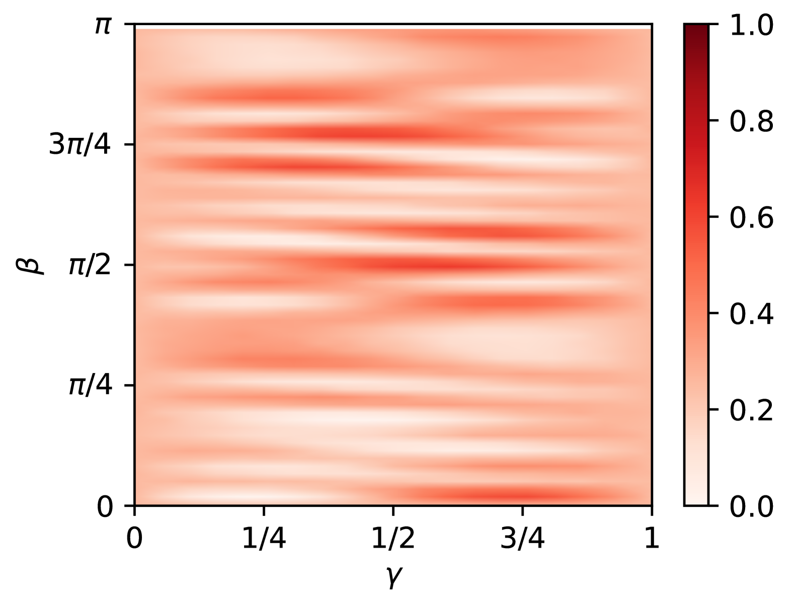
Figure 4: Plotting the the probability to successfully refine the solution (indicative of the underlying optimisation landscape) over a pair of parameters $(\gamma,\beta)$ in a $p=1$ layer QAOA for a random 3-qubit problem instance.

Ahead of our experimentation, we pre-train $p$-deep QAOA circuits according to alg. 1 for $p=1,\dots,10$. The validation performances at each epoch are shown in fig. 5, showing general improvement for increasing $p$.

Discussion and prospective results are given for alternative training schemes in appendix C.

Validation ‘Loss’ Curves for Angle Pre-training

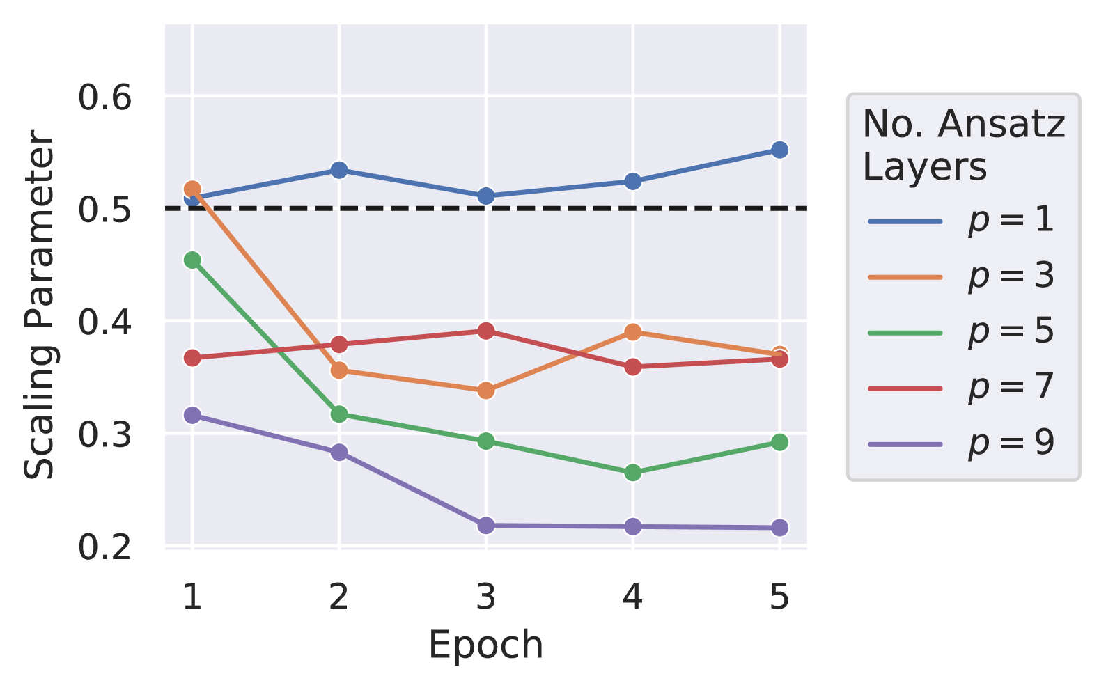
Figure 5: Validation performance during the pre-training of $p$-depth QAOA circuits. The ‘loss’ being minimised is the scaling parameter $\alpha$ in the curve $q(n)=1/2^{\alpha n}$ over a dataset of validation points $(n_{i},q_{i})$. The dashed line denotes the speed-up offered by Grover’s algorithm [60].

Separately, we train a large number of $p=1$ layer QAOA circuits independently for random CVP instances and make note of the obtained values for $\beta$ and $\gamma$. We may plot these by the instance size, as shown in fig. 6, to observe the convergence of the angles for growing problem complexity. An indicative optimisation (for a small instance) landscape is exemplified by fig. 4, though the landscape becomes increasingly flat as the problem complexity (here, lattice dimension) grows – the dreaded “barren plateau” phenomenon [63, 64, 65, 66, 67].

Convergence of QAOA Angles by Bit-length

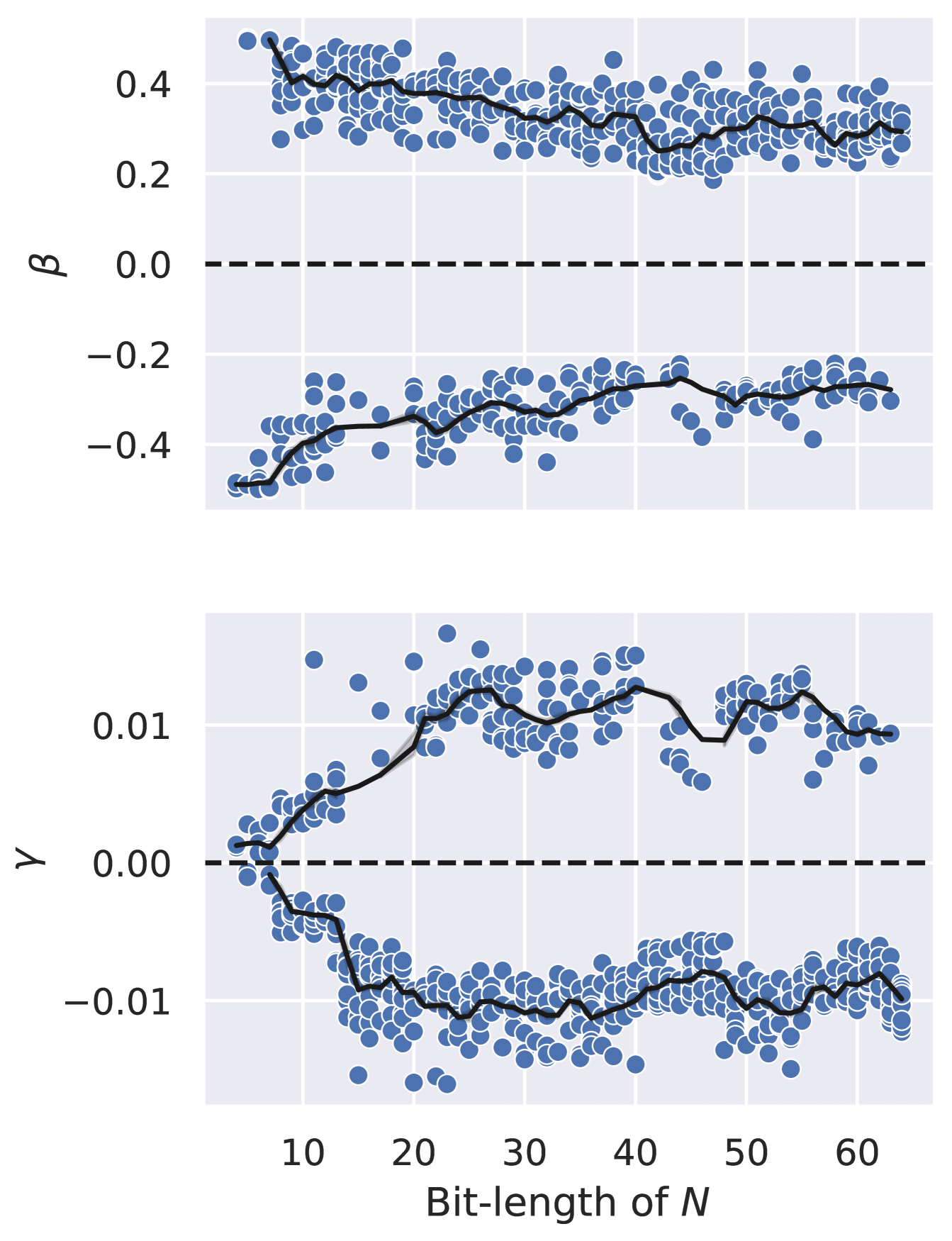
Figure 6: Convergence of the angles in a $p=1$ layer QAOA over different instances of varying bit-length.

From fig. 6, we gain confidence that a stable set of angles can be easily learnt, and that they will have the capacity to scale to larger instances without the necessity to re-train nor fine-tune.

Fig. 6 also highlights the issue of overfitting extremely well. Suppose we had followed a method similar to that of Brandao et al. [40] and selected a single small instance on which to find our angles. The angles found on these smaller problems are not yet converged, unlike with later cases, and so are less likely to generalise well. Then any small instance we select will provide angles that are suboptimal in general. Hence, our scheme is advantageous in being aware of convergence and overfitting.

V.2 Obtaining Statistics

For our experiments, we conduct a broad numerical analysis to determine the trending relationship between refinement probability and lattice dimension, which then implies time-complexity via the expected number of queries to the QAOA circuit. Cases wherein the approximately found solution already represents the best solution in the unit neighbourhood are omitted.

First, generate a CVP for the $n$-dimensional lattice $\mathcal{L}(B_{n,c})$ for an $m$-bit composite integer $N$, where $n=m/\log m$ as specified by Schnorr [32]. The method in Yan et al. [1] is only exemplified for three cases, however we simulate on the order of tens of thousands of cases so that an accurate scaling curve may be plotted to indicate asymptotic runtime.

We implement the QAOA solving a minimum-eigenstate problem for the Hamiltonian $\hat{H}_{C}$, as detailed in section IV.2, to obtain an outcome measurement $|\psi\rangle$ representing a binary string $\psi$ deciding whether to ‘step’ in each of the reduced basis directions $D=[\mathbf{d}_{1},\dots,\mathbf{d}_{n}]$ from $\mathbf{b}_{op}$. Hence, we may translate any $|\psi\rangle$ into the corresponding lattice vector $\mathbf{v}_{new}$ by performing $\mathbf{b}_{op}+\kappa\circ\psi D$, where $\circ$ denotes element-wise multiplication.

The probability to refine the solution (i.e. sample an improvement over $\mathbf{b}_{op}$) is ascertained by aggregating the probabilities for each $|\psi\rangle\mapsto\mathbf{v}_{new}$ for which $\|\mathbf{t}-\mathbf{v}_{new}\|^{2}<\|\mathbf{t}-\mathbf{b}_{op}\|^{2}$. This is the statistic whose decay we work to reduce with increasing lattice dimension $n$.

V.3 Complexity Analysis for the Refinement

Obtaining statistics for greatly many instances produces a dataset of points $(n_{i},q_{i})$, where $n_{i}=\log N_{i}/\log\log N_{i}$ is the ‘exact’ lattice dimension computed directly from the composite integer $N_{i}$, and $q_{i}$ is the estimated probability to refine the approximation (obtained classically by the method in section IV.1). From $q_{i}$, we can expect to make $1/q_{i}$ queries to the circuit to yield the desired solution.

These statistics are obtained by QAOA circuits of depths $p=1,\dots,10$ and plotted in fig. 2. In each case, we consider bit-lengths $4\leq m\leq 128$, and thus lattice dimensions $3\leq n\leq 18$. This is substantially larger than is considered in Yan et al. [1], and should be large enough to reveal any scalability concerns [34, 36, 35, 37].

Our optimal scaling is obtained, unsurprisingly, by $p=10$ layers, relating the refinement probability to lattice dimension as $q(n)\approx 1/2^{0.225n}$, and thus indicating a time-complexity scaling as $O(2^{0.225n})$. This is more than a quadratic speed-up over the famous Grover’s algorithm [60], with far shallower depth and without requirement for fault tolerance. These findings mimic that of Boulebnane and Montanaro [39] for the improvement over Grover by fixed angles for QAOA. In fact, we find improvement with any depth $p>2$.

Our results indicate a promising relationship between the scaling parameter $\alpha$, which characterises the degree of the exponential decay by $1/2^{\alpha n}$, and the lattice dimension $n$. Fig. 7 fits an exponential curve to this relationship and extrapolates to greater depths. Optimistically, we estimate that the time complexity will reduce to $O(2^{0.1n})$ for $p>20$.

Relationship Between Scaling $\alpha$ and Depth $p$

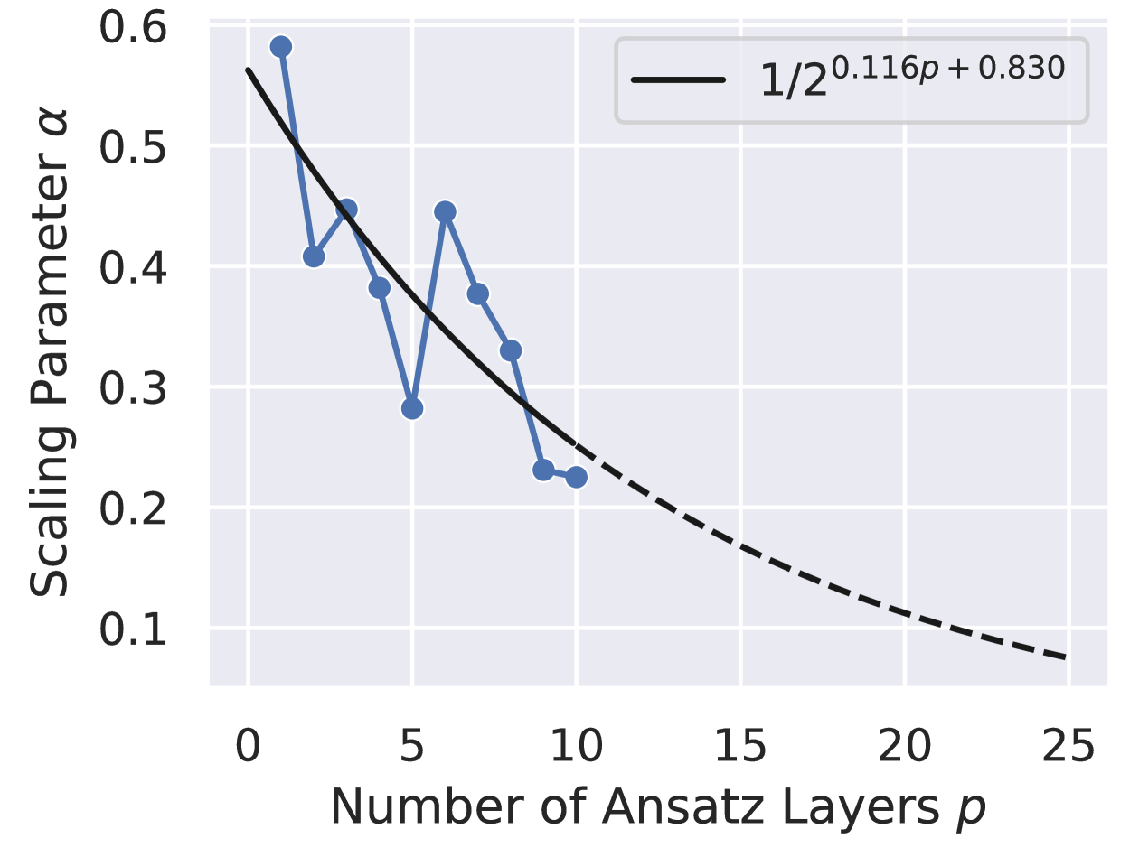
Figure 7: Extrapolating the relationship between the optimal scaling obtainable at each QAOA depth $p$, taken from fig. 2.

V.4 Refinement Quality

We will take brief notice of the scaling of the quality of the refinement in fig. 8. While the improvement may appear small, we must note that any improvement is significant due to the discrete nature of $\mathcal{L}$ – an improvement indicates that an entirely different sr-pair has been identified, which comes with a different likelihood for usefulness in cryptography.

Quality of the Refinement by Lattice Dimension

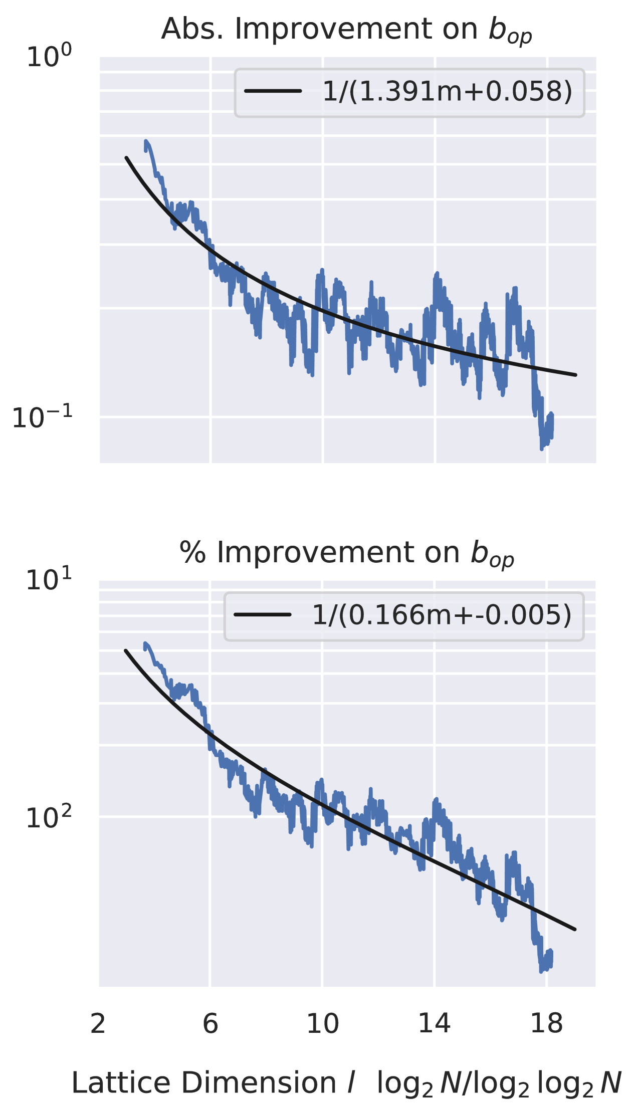
Figure 8: The improvement that the best solution in the neighbourhood obtains over $\mathbf{b}_{op}$ with increasing lattice dimension. A rolling average is given and a best-fit curve is shown.

The quality of available solutions with this method is a primary concern in Grebnev et al. [34], and is noted by other literature [36, 35]. We consider data for which a refinement exists (i.e. situations in which the unit neighbourhood around $\mathbf{b}_{op}$ contains a better solution), and note a subexponential decay of quality in fig. 8. However, it is still unlikely that this quality is sufficient for sieving and thus factoring.

We are optimistic that, given our findings for the potential quantum advantage in reducing the decay of refinement probability, the search space may be increased by dropping Schnorr [32]’s contentious sublinear lattice dimension scheme (see appendix B).

VI Conclusion

In this work, we proposed a simple yet robust pre-training algorithm to use for fixed-angles QAOA. The method has been used on lattice-based problems, and enabled a heuristic analysis of the time-complexity of QAOA for sieving on the prime lattice [30, 31, 32].

Extending from the method in Yan et al. [1] for refining approximations to the closest vector problem as a reduction for the sieving problem, we indicate the possibility for a quantum advantage in searching for refinements via a fixed angle scheme for QAOA. In doing this, we hope to reveal the threat posed by newer variational approaches to lattice problems in cryptography.

Further work should explore whether this potential advantage persists as the search space for refinement grows – say, for a neighbourhood encoding in $O(n\log n)$ qubits rather than $O(n)$. If the advantage is not lost in larger spaces, then lattice problems may be sufficiently challenged by these heuristic search methods, provided a set of angles can generalise well across instances. For a large enough neighbourhood (which is, in itself, not trivial to determine), there may be potential to find exact solutions with a reasonable exponent in the time-complexity, though we expected that a highly constrained lattice should be assumed for such optimism. The prime lattice may be sufficiently constrained for explorations in this direction.

VI.1 Limitations

Beyond the limitation due to insufficient search space, which has been discussed previously in connection with Yan et al. [1] and Schnorr [32] regarding their “sublinear factoring” claim (see appendix B), there are two limitations in this work that it is worth reiterating as a motivation for future research.

First, we only consider CVPs constructed on the prime lattice, as by their very nature (see section IV), they are focused on sieving for sr-pairs. This gives our work a strong flavour of cryptanalysis, which serves as the main interest for finding a quantum advantage for lattice problems, though it may be argued to lack generality. Indeed, our success in finding a good set of angles may not be replicated with ease in more general CVPs, in which the structure has greater variance.

Second, this work simulates quantum circuitry without considering the effect of noise. By working with relatively shallow-depth QAOA circuits, we remain optimistic that our findings can be experimentally ratified with real quantum hardware, perhaps with smaller advantage. We note that overly noisy hardware confounds the process of pre-training beyond practical use. We also note, however, that our algorithm can also be viewed as an early fault-tolerant one, since our approach could be applied to error-corrected circuits and would be better than, for example, naive Grover-type approaches, both in terms of time-complexity, and in terms of concrete number of logical qubits required (space-complexity).

Appendix A Lattice Reduction

The difficulty of any lattice problem is dictated in large part by the ‘quality’ of the given basis $B$. A ‘good’ basis is one consisting of short, relatively mutually orthogonal vectors, making navigation precise and intuitive. On the other hand, a ‘bad’ basis consists of long, relatively mutually parallel vectors that confound the method of walking toward particular points by combinations of basis vectors. This intuition leads to public-key cryptosystems on lattices, for which a pair of good and bad bases imply private and public keys.

Ideally then, we should like to start with a good basis, even if we are given a bad one to work from. The process of making a given basis ‘better’ is referred to as lattice reduction. Useful literature for developing an intuitive understanding for lattice reduction algorithms in cryptanalysis include Joux and Stern [68], Nguyen and Stern [69], and Bremner [70] in particular for an introduction.

In this work, we consider the famous LLL-reduction algorithm due to Lenstra et al. [61]. For convenience, we give a brief description here. Useful texts include those aforementioned, or Wübben et al. [71]. Discussion here draws also from Schnorr [32].

Definition A.1 (QR-decomposition)

Any basis matrix $B$ has the unique decomposition $B=QR$, where $Q\in\mathbb{R}^{n\times m}$ is isometric (with pairwise orthogonal column vectors of unit length) and $R=[r_{i,j}]_{1\leq i,j\leq m}\in\mathbb{R}^{m\times m}$ is upper triangular with positive diagonal entries $r_{i,i}$.

Furthermore, $R=\text{GNF}(B)$ is the generic normal form of $B$, whose Gram-Schmidt coefficients $\mu_{j,i}=r_{i,j}/r_{i,i}$ are rational for integer matrices.

Definition A.2 (LLL Reduction)

A basis $B$ is $\delta$-LLL reduced, if $|\mu_{i,j}|$ for all $i<j$, and $\delta r^{2}_{i,i}\leq r^{2}_{i,i+1}+r^{2}_{i+1,i+1}$ for $i=1,\dots,n-1$.

We enforce that $\frac{1}{4}<\delta\leq 1$. Lenstra et al. [61] show that any basis can be $\delta$-LLL reduced for $\delta<1$ in polynomial time, and that they approximate the successive minima well.

Appendix B Sublinearity of Schnorr’s Method

This section provides supplementary detail for the lattice dimension scheme presented by Schnorr [30, 31, 32] that gives rise to the sublinearity claim later championed in Schnorr [32] and Yan et al. [1] to “destroy the RSA cryptosystem”. We then discuss the evidence against the validity of this scheme [34, 36, 35, 37], with particular focus on the findings of Aboumrad et al. [35].

B.1 The Sublinear Scheme

By Minkowski’s first theorem (see [72]), the shortest vector $\lambda_{1}$ for any full rank $n$-dimensional lattice $\mathcal{L}\subseteq\mathbb{R}^{n}$ is bounded from above as

$$\lambda_{1}(\mathcal{L})^{2}\leq n\cdot(\det\mathcal{L})^{2/n}\ .$$ (16)

The discrepancy between the real shortest vector $\lambda_{1}$ and this bound can be measured by the relative density $\text{rd}(\mathcal{L})$ of the lattice, which gives a ratio between $\lambda_{1}$ and the upper bound estimated by the Hermite constant;

$$\text{rd}(\mathcal{L}):=\frac{\lambda_{1}(\mathcal{L})}{\sqrt{\gamma_{n}}(\det\mathcal{L})^{1/n}}\ ,$$ (17)

where $\gamma_{n}$ is the Hermite constant of definition II.6.

Schnorr [30] made the critical assumption that a random lattice $\mathcal{L}$ with size-ordered basis $B=[\mathbf{b}_{1},\dots,\mathbf{b}_{m}]$ has a relative density satisfying

$$\text{rd}(\mathcal{L})\leq\bigg{(}\sqrt{\frac{e\pi}{2n}}\cdot\frac{\lambda_{1}(\mathcal{L})}{\|\mathbf{b}_{1}\|}\bigg{)}^{1/2}\ ,$$ (18)

and since $\lambda_{1}(\mathcal{L})\|/\mathbf{b_{1}}\|\leq 1$, this then leads to

$$\text{rd}(\mathcal{L})=\frac{\lambda_{1}(\mathcal{L})}{\sqrt{\gamma_{n}}(\det\mathcal{L})^{1/n}}\leq\bigg{(}\frac{e\pi}{2n}\bigg{)}^{1/4}\ .$$ (19)

We can then propose that, for the lattice $\mathcal{L}(B_{n,c})$ whose dimension satisfies $n=2c\log N/\log\log N$, and whose relative density satisfies eq. (19), there exists some vector $\mathbf{v}\in\mathcal{L}(B_{n,c})$ such that $\|\mathbf{v}-\mathbf{t}\|^{2}=O(\log N)$ for any target vector $\mathbf{t}\in\text{Span}(B_{n,c})$. Proofs for this proposition are given in Schnorr [32] and in the appendix of Yan et al. [1].

B.2 Validity of the Scheme and Assumption

Firstly, the sublinear scheme is only of practical use if the reduction from factoring to the search for sr-pairs works in polynomial time, given the heuristic assumptions of density culminating in eq. (19). Practical implementations, such as Ducas [37], dispute that this assumption successfully scales well enough to be cryptographically significant. Theoretical considerations tend to agree with this disputatious attitude [34].

Secondly, since the foundations of Schnorr [30]’s guarantees were formulated in the early 1990s, the theory of lattice problems has developed tremendously, including the reliance of most popular CVP heuristics on $\ell_{2}$-measurements (e.g. [73]). This leaves the proofs in Schnorr [30] (in particular, Lemma 2) with limited practical bearing [35].

Thirdly, Aboumrad et al. [35] use theoretic results [74, 75] to estimate the density of $p_{N}$-smooth numbers as $N$ grows (note that $p_{N}$-smooth here refers to integers whose prime factors are not greater than $N$). Combining Dickman’s function with the prime number theorem allows them to estimate that the proportion of $p_{N}$-smooth numbers below $N$ that may be collected under the sublinear lattice dimension scheme is exponentially small (see section 3.1 of Aboumrad et al. [35]).

For small $N$, the assumption is acceptable, but the exponential decay of available smooth numbers renders the assumption unacceptable for large $N$, and hence the scalability of Schnorr’s method [30, 31, 32] should be doubted under a sublinear scheme. This decay is the primary cause for the necessity for exponentially many CVP instances needing to be solved for a factorisation to be possible – we need exponentially many solutions to be sure of finding enough unique sr-pairs for post-processing.

Using a Single CVP Instance to Find and Fix Angles

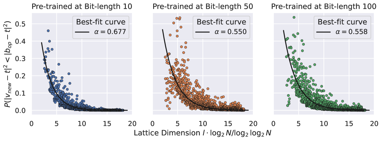
Figure 9: Probability to refine the approximate solution by lattice dimension for three distinct QAOA circuits with angles specified by a single (random) instance. The size of these instance (given in bit-length of $N$) is indicated above each plot.

Optimising Each CVP Instance Independently (No Pretraining)

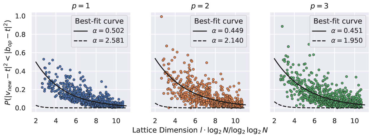
Figure 10: Similarly to fig. 9, though without any pre-training scheme. That is, each instance of the QAOA obtains its angles independently. We show here also a dashed line representing the scaling when also considering cases in which no refinement exists within the neighbourhood.

Appendix C Alternative Angle Selection Schemes

This appendix presents some prospective results for our scaling analysis with alternative methods for angle selection. This serves to contextualise the success of our proposed pre-training scheme.

C.1 Random Instance Pre-training

The most straightforward way to obtain angles – short of drawing them randomly – is to train on a single (random) instance and take the consequent angles. This is the impression left by Brandao et al. [40].

Ideally, the single instance we choose as our pre-training instance is small enough that the angles may be obtained relatively efficiently, but large enough that the resultant angles are general (see fig. 6 to get a sense for the convergence of the angles by instance size).

Fig. 9 gives the time complexity (mimicking the subplots in fig. 2) one might expect to obtain in general having pre-trained by a single random instance at the indicated size. This is roughly inline with our expectation that bit-lengths $<20$ are ineffective for obtaining generalisable angles. We further notice that increasing bit-length does not appear to continue reducing the probability decay.

Our preliminary conclusion is that pre-training by a single random instance has the limit of Grover’s speed up ($\alpha\approx\frac{1}{2}$). More instances are required to gather the information necessary to find general angles, as in our proposed scheme in section IV.

C.2 No Pre-training

We would also like to show propsective results from a lack of pre-training altogether. Here, we obtain the angles in each instance independently, as is currently standard in QAOA.

This, of course, results in immense computational effort when considering greatly many instances as we do, hence we are unable to explore to the largest lattice dimensions. Already, this is a decisive difference between a fixed angle scheme and the absence thereof – when you are happy to omit the optimisation of angles, we can set out immediately querying the circuit!

The prospective results, shown in fig. 10, are better than for random instance pre-training, though have a similar apprehension for continued improvement. The improvement over random instance pre-training is expected (after all, each instance finds its own ‘perfect’ angles), but an overall lack of improvement over our own pre-training scheme (see fig. 2) is surprising. Indeed, exploring to greater depths may be the deciding factor in demonstrating an ability to withstand the exponential decay of probability.

Again, we conclude that pre-training is an indispensable tool in the usage of QAOA, and leads to the potential for a quantum advantage that we highlight in this work.

Appendix D Implementation Details

Our work was produced in Python (version 3.8.18), and is available at [42].

LLL-reduction [61] and Babai’s nearest plane algorithm [47] are implemented via FPyLLL (version 0.6.1; [76]), a Python interface for the lattice algorithm library FPLLL (version 5.4.5; [77]). This further relied on NumPy (version 1.22.3; [78]).

For the quantum portion of our implementation, we use Google Cirq (version 1.1.0; [79]) and the accompanying qsimcirc (version 0.18.0; [80]) for simulation. Unfortunately, Cirq does not provide an implementation of QAOA (yet), so we have derived our own implementation from Khattar and Yosri [36].

For the results presented in this work, we use the Nelder-Mead simplex algorithm [81] for minimisation of the expectation values of the observables in our circuit via SciPy (version 1.10.1; [82]).

References

- Yan et al. [2022] B. Yan, Z. Tan, S. Wei, H. Jiang, W. Wang, H. Wang, L. Luo, Q. Duan, Y. Liu, W. Shi, Y. Fei, X. Meng, Y. Han, Z. Shan, J. Chen, X. Zhu, C. Zhang, F. Jin, H. Li, C. Song, Z. Wang, Z. Ma, H. Wang, and G.-L. Long, Factoring integers with sublinear resources on a superconducting quantum processor (2022), arXiv:2212.12372 [quant-ph] .
- Rivest et al. [1978] R. L. Rivest, A. Shamir, and L. Adleman, A method for obtaining digital signatures and public-key cryptosystems, Communications of the ACM 21, 120 (1978).
- Zhang et al. [2024] D. Zhang, H. Wang, S. Li, and B. Wang, Progress in the prime factorization of large numbers, The Journal of Supercomputing , 1 (2024).
- Shor [1995] P. W. Shor, Polynomial-time algorithms for prime factorization and discrete logarithms on a quantum computer, SIAM Rev. 41, 303 (1995).
- Lucero et al. [2012] E. Lucero, R. Barends, Y. Chen, J. Kelly, M. Mariantoni, A. Megrant, P. O’Malley, D. Sank, A. Vainsencher, J. Wenner, T. White, Y. Yin, A. N. Cleland, and J. M. Martinis, Computing prime factors with a josephson phase qubit quantum processor, Nature Physics 8, 719–723 (2012).
- Lanyon et al. [2007] B. P. Lanyon, T. J. Weinhold, N. K. Langford, M. Barbieri, D. F. V. James, A. Gilchrist, and A. G. White, Experimental demonstration of a compiled version of shor’s algorithm with quantum entanglement, Physical Review Letters 99, 10.1103/physrevlett.99.250505 (2007).
- Lu et al. [2007] C.-Y. Lu, D. E. Browne, T. Yang, and J.-W. Pan, Demonstration of a compiled version of shor’s quantum factoring algorithm using photonic qubits, Physical Review Letters 99, 10.1103/physrevlett.99.250504 (2007).
- Martín-López et al. [2012] E. Martín-López, A. Laing, T. Lawson, R. Alvarez, X.-Q. Zhou, and J. L. O’Brien, Experimental realization of shor’s quantum factoring algorithm using qubit recycling, Nature Photonics 6, 773–776 (2012).
- Bernstein and Lange [2017] D. J. Bernstein and T. Lange, Post-quantum cryptography, Nature 549, 188 (2017).
- Goldreich et al. [1997] O. Goldreich, S. Goldwasser, and S. Halevi, Public-key cryptosystems from lattice reduction problems, in Advances in Cryptology—CRYPTO’97: 17th Annual International Cryptology Conference Santa Barbara, California, USA August 17–21, 1997 Proceedings 17 (Springer, 1997) pp. 112–131.
- Hoffstein et al. [1998] J. Hoffstein, J. Pipher, and J. H. Silverman, Ntru: A ring-based public key cryptosystem, in International algorithmic number theory symposium (Springer, 1998) pp. 267–288.
- Hoffstein et al. [2001] J. Hoffstein, J. Pipher, and J. H. Silverman, Nss: An ntru lattice-based signature scheme, in Advances in Cryptology—EUROCRYPT 2001: International Conference on the Theory and Application of Cryptographic Techniques Innsbruck, Austria, May 6–10, 2001 Proceedings 20 (Springer, 2001) pp. 211–228.
- Hoffstein et al. [2003] J. Hoffstein, N. Howgrave-Graham, J. Pipher, J. H. Silverman, and W. Whyte, Ntrusign: Digital signatures using the ntru lattice, in Cryptographers’ track at the RSA conference (Springer, 2003) pp. 122–140.
- Lyubashevsky [2012] V. Lyubashevsky, Lattice signatures without trapdoors, in Annual International Conference on the Theory and Applications of Cryptographic Techniques (Springer, 2012) pp. 738–755.
- Ducas et al. [2013] L. Ducas, A. Durmus, T. Lepoint, and V. Lyubashevsky, Lattice signatures and bimodal gaussians, in Annual Cryptology Conference (Springer, 2013) pp. 40–56.
- Bernstein et al. [2018] D. J. Bernstein, C. Chuengsatiansup, T. Lange, and C. van Vredendaal, Ntru prime: reducing attack surface at low cost, in Selected Areas in Cryptography–SAC 2017: 24th International Conference, Ottawa, ON, Canada, August 16-18, 2017, Revised Selected Papers 24 (Springer, 2018) pp. 235–260.
- Coppersmith and Shamir [1997] D. Coppersmith and A. Shamir, Lattice attacks on ntru, in International conference on the theory and applications of cryptographic techniques (Springer, 1997) pp. 52–61.
- Nguyen and Regev [2006] P. Q. Nguyen and O. Regev, Learning a parallelepiped: Cryptanalysis of ggh and ntru signatures, in Annual international conference on the theory and applications of cryptographic techniques (Springer, 2006) pp. 271–288.
- Ducas and Nguyen [2012] L. Ducas and P. Q. Nguyen, Learning a zonotope and more: Cryptanalysis of ntrusign countermeasures, in International Conference on the Theory and Application of Cryptology and Information Security (Springer, 2012) pp. 433–450.
- Laarhoven [2015] T. Laarhoven, Sieving for shortest vectors in lattices using angular locality-sensitive hashing, in Advances in Cryptology–CRYPTO 2015: 35th Annual Cryptology Conference, Santa Barbara, CA, USA, August 16-20, 2015, Proceedings, Part I 35 (Springer, 2015) pp. 3–22.
- Laarhoven and de Weger [2015] T. Laarhoven and B. de Weger, Faster sieving for shortest lattice vectors using spherical locality-sensitive hashing, in Progress in Cryptology–LATINCRYPT 2015: 4th International Conference on Cryptology and Information Security in Latin America, Guadalajara, Mexico, August 23-26, 2015, Proceedings 4 (Springer, 2015) pp. 101–118.
- Becker et al. [2016] A. Becker, L. Ducas, N. Gama, and T. Laarhoven, New directions in nearest neighbor searching with applications to lattice sieving, in Proceedings of the twenty-seventh annual ACM-SIAM symposium on Discrete algorithms (SIAM, 2016) pp. 10–24.
- Alagic et al. [2022] G. Alagic, G. Alagic, D. Apon, D. Cooper, Q. Dang, T. Dang, J. Kelsey, J. Lichtinger, Y.-K. Liu, C. Miller, et al., Status report on the third round of the nist post-quantum cryptography standardization process, CSRC (2022).
- Computer Security Division [2017] I. T. L. Computer Security Division, Post-quantum cryptography standardization - post-quantum cryptography: Csrc (2017).
- Pomerance [1984] C. Pomerance, The quadratic sieve factoring algorithm, in Workshop on the Theory and Application of of Cryptographic Techniques (Springer, 1984) pp. 169–182.
- Davis and Holdridge [1984] J. A. Davis and D. B. Holdridge, Factorization using the quadratic sieve algorithm, in Advances in Cryptology: Proceedings of Crypto 83, edited by D. Chaum (Springer US, Boston, MA, 1984) pp. 103–113.
- Lenstra and Lenstra [1993] A. K. Lenstra and H. W. Lenstra, The development of the number field sieve, Vol. 1554 (Springer Science & Business Media, 1993).
- Briggs [1998] M. E. Briggs, An introduction to the general number field sieve, Ph.D. thesis, Virginia Tech (1998).
- Boudot et al. [2022] F. Boudot, P. Gaudry, A. Guillevic, N. Heninger, E. Thomé, and P. Zimmermann, The state of the art in integer factoring and breaking public-key cryptography, IEEE Security & Privacy 20, 80 (2022).
- Schnorr [1991] C. P. Schnorr, Factoring integers and computing discrete logarithms via diophantine approximation, in Advances in Cryptology — EUROCRYPT ’91, edited by D. W. Davies (Springer Berlin Heidelberg, Berlin, Heidelberg, 1991) pp. 281–293.
- Schnorr [2013] C. P. Schnorr, Factoring integers by cvp algorithms, Number Theory and Cryptography: Papers in Honor of Johannes Buchmann on the Occasion of His 60th Birthday , 73 (2013).
- Schnorr [2021] C. P. Schnorr, Fast factoring integers by svp algorithms, corrected, Cryptology ePrint Archive, Paper 2021/933 (2021), https://eprint.iacr.org/2021/933.
- Farhi et al. [2014] E. Farhi, J. Goldstone, and S. Gutmann, A quantum approximate optimization algorithm, arXiv preprint arXiv:1411.4028 (2014).
- Grebnev et al. [2023] S. V. Grebnev, M. A. Gavreev, E. O. Kiktenko, A. P. Guglya, A. R. Efimov, and A. K. Fedorov, Pitfalls of the sublinear qaoa-based factorization algorithm, IEEE Access 11, 134760–134768 (2023).
- Aboumrad et al. [2023] W. Aboumrad, D. Widdows, and A. Kaushik, Quantum and classical combinatorial optimizations applied to lattice-based factorization, arXiv preprint arXiv:2308.07804 (2023).
- Khattar and Yosri [2023] T. Khattar and N. Yosri, A comment on” factoring integers with sublinear resources on a superconducting quantum processor”, arXiv preprint arXiv:2307.09651 (2023).
- Ducas [2021] L. Ducas, Lducas/schnorrgate: Testing schnorr’s factorization claim in sage (2021).
- Vera [2010] A. I. Vera, A note on integer factorization using lattices, arXiv preprint arXiv:1003.5461 (2010).
- Boulebnane and Montanaro [2022] S. Boulebnane and A. Montanaro, Solving boolean satisfiability problems with the quantum approximate optimization algorithm (2022), arXiv:2208.06909 [quant-ph] .
- Brandao et al. [2018] F. G. S. L. Brandao, M. Broughton, E. Farhi, S. Gutmann, and H. Neven, For fixed control parameters the quantum approximate optimization algorithm’s objective function value concentrates for typical instances (2018), arXiv:1812.04170 [quant-ph] .
- Prokop and Wallden [2025] M. Prokop and P. Wallden, Heuristic time complexity of nisq shortest-vector-problem solvers (2025), arXiv:2502.05284 [quant-ph] .
- Priestley [2025] B. Priestley, Code for the paper: A practical scalable approach to the cvp for sieving via qaoa with fixed angles, https://github.com/BenPrie/qaoa-for-cvp (2025).
- Note [1] We note that this does not conflict any known results on the asymptotic optimality of Grover, since QAOA is not a “black-box” oracle algorithm and uses the structure of the problem (via the problem Hamiltonian) in the way the ansatz is constructed.
- Cerezo et al. [2021a] M. Cerezo, A. Arrasmith, R. Babbush, S. C. Benjamin, S. Endo, K. Fujii, J. R. McClean, K. Mitarai, X. Yuan, L. Cincio, et al., Variational quantum algorithms, Nature Reviews Physics 3, 625 (2021a).
- Albrecht et al. [2023] M. R. Albrecht, M. Prokop, Y. Shen, and P. Wallden, Variational quantum solutions to the Shortest Vector Problem, Quantum 7, 933 (2023).
- Joseph et al. [2021] D. Joseph, A. Callison, C. Ling, and F. Mintert, Two quantum ising algorithms for the shortest-vector problem, Phys. Rev. A 103, 032433 (2021).
- Babai [1986] L. Babai, On lovász’lattice reduction and the nearest lattice point problem, Combinatorica 6, 1 (1986).
- Kraitchik [1922] M. Kraitchik, Théorie des nombres, Vol. 1 (Gauthier-Villars, 1922).
- Morrison and Brillhart [1975] M. A. Morrison and J. Brillhart, A method of factoring and the factorization of f7, Mathematics of computation 29, 183 (1975).
- Dixon [1981] J. D. Dixon, Asymptotically fast factorization of integers, Mathematics of computation 36, 255 (1981).
- Bennett [2023] H. Bennett, The complexity of the shortest vector problem, SIGACT News 54, 37–61 (2023).
- Regev [2005] O. Regev, On lattices, learning with errors, random linear codes, and cryptography, in Proceedings of the Thirty-Seventh Annual ACM Symposium on Theory of Computing, STOC ’05 (Association for Computing Machinery, New York, NY, USA, 2005) p. 84–93.
- Bennett et al. [2017] H. Bennett, A. Golovnev, and N. Stephens-Davidowitz, On the quantitative hardness of cvp, in 2017 IEEE 58th Annual Symposium on Foundations of Computer Science (FOCS) (IEEE, 2017) pp. 13–24.
- Micciancio [2001] D. Micciancio, The hardness of the closest vector problem with preprocessing, IEEE Transactions on Information Theory 47, 1212 (2001).
- Micciancio and Goldwasser [2002] D. Micciancio and S. Goldwasser, Complexity of lattice problems: a cryptographic perspective, Vol. 671 (Springer Science & Business Media, 2002).
- Farhi et al. [2000] E. Farhi, J. Goldstone, S. Gutmann, and M. Sipser, Quantum computation by adiabatic evolution, arXiv preprint quant-ph/0001106 (2000).
- Farhi et al. [2001] E. Farhi, J. Goldstone, S. Gutmann, J. Lapan, A. Lundgren, and D. Preda, A quantum adiabatic evolution algorithm applied to random instances of an np-complete problem, Science 292, 472 (2001).
- Zhou et al. [2020] L. Zhou, S.-T. Wang, S. Choi, H. Pichler, and M. D. Lukin, Quantum approximate optimization algorithm: Performance, mechanism, and implementation on near-term devices, Physical Review X 10, 10.1103/physrevx.10.021067 (2020).
- Bravyi et al. [2019] S. Bravyi, D. Browne, P. Calpin, E. Campbell, D. Gosset, and M. Howard, Simulation of quantum circuits by low-rank stabilizer decompositions, Quantum 3, 181 (2019).
- Grover [1996] L. K. Grover, A fast quantum mechanical algorithm for database search (1996), arXiv:quant-ph/9605043 [quant-ph] .
- Lenstra et al. [1982] A. K. Lenstra, H. W. Lenstra, and L. Lovász, Factoring polynomials with rational coefficients, Mathematische annalen 261, 515 (1982).
- Lucas [2014] A. Lucas, Ising formulations of many np problems, Frontiers in physics 2, 5 (2014).
- Wang et al. [2021] S. Wang, E. Fontana, M. Cerezo, K. Sharma, A. Sone, L. Cincio, and P. J. Coles, Noise-induced barren plateaus in variational quantum algorithms, Nature communications 12, 6961 (2021).
- Uvarov and Biamonte [2021] A. Uvarov and J. D. Biamonte, On barren plateaus and cost function locality in variational quantum algorithms, Journal of Physics A: Mathematical and Theoretical 54, 245301 (2021).
- Anschuetz and Kiani [2022] E. R. Anschuetz and B. T. Kiani, Quantum variational algorithms are swamped with traps, Nature Communications 13, 7760 (2022).
- Cerezo et al. [2021b] M. Cerezo, A. Sone, T. Volkoff, L. Cincio, and P. J. Coles, Cost function dependent barren plateaus in shallow parametrized quantum circuits, Nature communications 12, 1791 (2021b).
- Larocca et al. [2024] M. Larocca, S. Thanasilp, S. Wang, K. Sharma, J. Biamonte, P. J. Coles, L. Cincio, J. R. McClean, Z. Holmes, and M. Cerezo, A review of barren plateaus in variational quantum computing, arXiv preprint arXiv:2405.00781 (2024).
- Joux and Stern [1998] A. Joux and J. Stern, Lattice reduction: A toolbox for the cryptanalyst, Journal of Cryptology 11, 161 (1998).
- Nguyen and Stern [2000] P. Q. Nguyen and J. Stern, Lattice reduction in cryptology: An update, in International Algorithmic Number Theory Symposium (Springer, 2000) pp. 85–112.
- Bremner [2011] M. Bremner, Lattice basis reduction (CRC Press New York, 2011).
- Wübben et al. [2011] D. Wübben, D. Seethaler, J. Jalden, and G. Matz, Lattice reduction, IEEE Signal Processing Magazine 28, 70 (2011).
- Thompson [1996] A. C. Thompson, Minkowski geometry (Cambridge University Press, 1996).
- Ajtai [1998] M. Ajtai, The shortest vector problem in l2 is np-hard for randomized reductions, in Proceedings of the thirtieth annual ACM symposium on Theory of computing (1998) pp. 10–19.
- Ramaswami [1949] V. Ramaswami, On the number of positive integers less than x and free of prime divisors greater than xˆc, Project Euclid (1949).
- de Bruijn [1951] N. G. de Bruijn, On the number of positive integers and free of prime factors , Proceedings of the Koninklijke Nederlandse Akademie van Wetenschappen: Series A: Mathematical Sciences 54, 50 (1951).
- development team [2023a] T. F. development team, fpylll, a Python wrapper for the fplll lattice reduction library, Version: 0.6.1 (2023a), available at https://github.com/fplll/fpylll.
- development team [2023b] T. F. development team, fplll, a lattice reduction library, Version: 5.4.5 (2023b), available at https://github.com/fplll/fplll.
- Harris et al. [2020] C. R. Harris, K. J. Millman, S. J. van der Walt, R. Gommers, P. Virtanen, D. Cournapeau, E. Wieser, J. Taylor, S. Berg, N. J. Smith, R. Kern, M. Picus, S. Hoyer, M. H. van Kerkwijk, M. Brett, A. Haldane, J. F. del Río, M. Wiebe, P. Peterson, P. Gérard-Marchant, K. Sheppard, T. Reddy, W. Weckesser, H. Abbasi, C. Gohlke, and T. E. Oliphant, Array programming with NumPy, Nature 585, 357 (2020).
- Developers [2024] C. Developers, Cirq (2024).
- team and collaborators [2020] Q. A. team and collaborators, qsim (2020).
- Gao and Han [2012] F. Gao and L. Han, Implementing the nelder-mead simplex algorithm with adaptive parameters, Computational Optimization and Applications 51, 259 (2012).
- Virtanen et al. [2020] P. Virtanen, R. Gommers, T. E. Oliphant, M. Haberland, T. Reddy, D. Cournapeau, E. Burovski, P. Peterson, W. Weckesser, J. Bright, S. J. van der Walt, M. Brett, J. Wilson, K. J. Millman, N. Mayorov, A. R. J. Nelson, E. Jones, R. Kern, E. Larson, C. J. Carey, İ. Polat, Y. Feng, E. W. Moore, J. VanderPlas, D. Laxalde, J. Perktold, R. Cimrman, I. Henriksen, E. A. Quintero, C. R. Harris, A. M. Archibald, A. H. Ribeiro, F. Pedregosa, P. van Mulbregt, and SciPy 1.0 Contributors, SciPy 1.0: Fundamental Algorithms for Scientific Computing in Python, Nature Methods 17, 261 (2020).