A Precise Determination of $\alpha_{s}$ from the Heavy Jet Mass Distribution

Abstract

A global fit for $\alpha_{s}(m_{Z})$ is performed on available $e^{+}e^{-}$ data for the heavy jet mass distribution. The state-of-the-art theory prediction includes $\mathcal{O}(\alpha_{s}^{3})$ fixed-order results, N³LL^′ dijet resummation, N²LL Sudakov shoulder resummation, and a first-principles treatment of power corrections in the dijet region. Theoretical correlations are incorporated through a flat random-scan covariance matrix. The global fit results in $0.1145^{+0.0021}_{-0.0019}$, compatible with similar determinations from thrust and $C$-parameter. Dijet resummation is essential for a robust fit, as it engenders insensitivity to the fit-range lower cutoff; without resummation the fit-range sensitivity is overwhelming. In addition, we find evidence for a negative power correction in the trijet region if and only if Sudakov shoulder resummation is included.

One of the main targets of precision QCD is the measurement of the strong coupling at colliders. In this endeavor, studies of $e^{+}e^{-}$ event shapes such as thrust and heavy jet mass (HJM) have led to enormous progress in our understanding of the interface between perturbative and non-perturbative QCD. Intriguingly, attempts to extract $\alpha_{s}$ from HJM data consistently produced values well below that from thrust [1, 2, 3, 4, 5, 6, 7, 8, 9], and below the PDG average [10]. In recent years, a number of differences between HJM and thrust were observed. First, HJM (in contrast to thrust) has a left-Sudakov shoulder due to large logarithms as $\rho\to 1/3$ from below [11, 12]. Second, in a recent study of soft emissions from three-parton configurations [13, 14, 15, 16, 17] it was suggested that these yield a positive non-perturbative power correction for thrust, shifting the distribution to the right, but a negative one for HJM, shifting the distribution leftward. As we will discuss, there is evidence that the Shoulder and the negative shift are intertwined. Third, power corrections in moments of the HJM distribution depend on different non-perturbative parameters than the tail OPE [18], while in thrust the parameters are the same. In this study, we incorporate all these effects into an improved fit. In addition, we include a more sophisticated treatment of correlated theoretical uncertainties using a random-scan covariance matrix which is added to the experimental one in the fits. This treatment of uncertainties leads to results robust across a wide range of fit regions with $\chi^{2}/{\rm dof}\approx 1$.

Figure 1: Comparison of the theory prediction to data from five experiments at $Q=91.2$ GeV. Horizontal error bars indicate the sizes of the experimental bins.

Experimental data: Data on the heavy jet mass cross section are given as binned distributions by the aleph [19], delphi [20, 21, 22], jade [23], l3 [24, 25] opal [26, 27, 28], and sld [29] collaborations. These measurements comprise 50 datasets at $35$ different center-of-mass energies between $35$ GeV and $207$ GeV for a total of 700 experimental data points. Data at $Q=91.2$ GeV is shown compared to our best theory result in Fig. 1.

Experimental measurements are generally provided with statistical and systematic experimental uncertainties. To treat correlations among the latter, we employ the LEP QCD working group [19, 28] minimal overlap model. We denote the statistical and systematical uncertainty for each data point (bin) by $\Delta_{i}^{\rm stat}$ and $\Delta_{i}^{\rm sys}$, respectively. We denote by $D_{i}$ to which of the 50 datasets, defined by energy and experiment, data-point $i$ belongs. Then, the minimal-overlap experimental covariance matrix is

$$\sigma_{ij}^{\rm exp}=\delta_{ij}(\Delta_{i}^{\rm stat})^{2}+\delta_{D_{i}D_{j}}{\rm min}(\Delta_{i}^{\rm sys},\Delta_{j}^{\rm sys})^{2}\,.$$ (1)

That is, $\sigma_{ij}^{\rm exp}$ is block-diagonal by dataset. This model assumes a positive correlation of systematic uncertainties within each dataset.

Each dataset for HJM has a peak at some value of $\rho$. These values of the peak position, which are described by $\rho_{\text{peak}}=0.003+a_{\text{peak}}/Q$ with $a_{\text{peak}}=1.56$ GeV (cf. supplement Fig. 7), provide a quantitative indication of the scale at which the distribution becomes non-perturbative. We thus restrict our fits to $\rho Q\geq 3a_{\text{peak}}$ to keep safely away from the fully non-perturbative region. We also impose $\rho\leq 0.3$ on our fits to avoid analogous non-perturbative effects in the shoulder region as well as unknown higher fixed-order contributions which are relatively more important for higher values of $\rho$. There are 451 experimental data points whose entire bin satisfies $3a_{\text{peak}}/Q\leq\rho\leq 0.3$.

HJM Distribution: The HJM differential cross section factorizes in the dijet limit into a global hard factor $H_{\text{dij}}$ times the two-dimensional convolution of two one-dimensional jet functions $J_{1,2}$, and the two-dimensional soft and shape functions [30, 31, 32, 33, 34, 18]:

$${\rm d}\sigma_{\text{dij}}=H_{\text{dij}}\times J_{1}\times J_{2}\otimes S_{1,2}\otimes F^{\Xi}_{1,2}(\Omega_{1}^{\rho})\,.$$ (2)

Here, the hard, jet and soft functions include large-log resummation, and the shape function $F^{\Xi}_{1,2}$ is given by matrix elements of QCD operators. For our fits it suffices to take the shape function to depend on a single non-perturbative dijet parameter $\Omega_{1}^{\rho}$, which is of ${\cal O}(\Lambda_{\rm QCD})$, and defined in the R-gap scheme that cancels the leading renormalon of the partonic soft function, with reference scale $2\,{\rm GeV}$ [35, 36].

Around the symmetric trijet limit, the distribution also factorizes as [11, 12]

$${\rm d}\sigma_{\text{sh}}^{\text{pert}}=H_{\text{sh}}\times J_{1}\times J_{2}\times J_{3}\otimes S_{1,2,3}\,.$$ (3)

While dijet resummation can be done analytically, shoulder resummation requires a numerical Fourier transform from position to momentum space which is computationally expensive. Although no first-principles study has been performed of power corrections around the symmetric trijet configuration, we model those corrections with a non-perturbative shift parameter. That is, we take

$$\frac{{\rm d}\sigma_{\text{sh}}}{{\rm d}\rho}(\rho)=\frac{{\rm d}\sigma^{\text{pert}}_{\text{sh}}}{{\rm d}\rho}\biggl{(}\rho-\frac{\Theta_{1}}{Q}\biggr{)}\,.$$ (4)

Here $\Theta_{1}<0$ corresponds to a negative shift in the trijet region. This is natural, since the shoulder expansion is around $r=1/3-\rho$, so a positive/physical non-perturbative shift in $r$ pushes the distribution to smaller $\rho$, and thus has $\Theta_{1}<0$.

Matching between the dijet, fixed-order and shoulder regions is done by writing the full cross section as

$${\rm d}\sigma=\Bigl{[}{\rm d}\sigma_{\text{dij}}-{\rm d}\sigma_{\text{dij}}^{\text{sing}}\Bigr{]}+{\rm d}\sigma_{\text{FO}}+\Bigl{[}{\rm d}\sigma_{\text{sh}}-{\rm d}\sigma_{\text{sh}}^{\text{sing}}\Bigr{]}\,.$$ (5)

Here ${\rm d}\sigma_{\rm FO}$ is fixed-order, known currently to ${\cal O}(\alpha_{s}^{3})$ [37, 38, 39, 40], while ${\rm d}\sigma_{\rm dij}$ and ${\rm d}\sigma_{\rm sh}$ resum large logarithms. ${\rm d}\sigma^{\text{sing}}_{X}$ refers to ${\rm d}\sigma_{X}$ with the jet, soft and hard scales set equal. With equal scales, each distribution reduces to a set of fixed-order terms involving $\ln^{k}(\rho)$ or $\ln^{k}(1/3-\rho)$. The differences in brackets are power suppressed in regions where their logarithms are not large. When logarithms are large, the ${\rm d}\sigma^{\text{sing}}_{X}$ subtract terms from ${\rm d}\sigma_{\rm FO}$ and avoid double counting. In practice, all regions overlap, so the interpolation between regions is handled by modulating the hard, jet and soft scales with profile functions $\mu_{i}(\rho)$. Profile functions for HJM have been discussed extensively elsewhere [41, 18, 12]. We summarize our choice of profiles in the supplemental material, providing the variation intervals of their parameters in Table 1.

To compare to the experimental data, the theory prediction should be integrated over each experimental bin. A practical implementation of this integration is by using the cumulative cross section in which the renormalization scales are set to the profiles evaluated at the center of the bin [35]. This avoids an expensive numerical integration over the dijet region, cancels large contributions from the peak region, and is as accurate as a direct integration within the order in perturbation theory one is working.

Fit Procedure: There is no standard way to estimate theoretical uncertainties, or to include theoretical uncertainties in fits to experimental data. A typical procedure is to perform a fit by minimizing $\chi^{2}$ using the experimental covariance matrix for various choices of theory parameters and estimating the theory uncertainty from the variation of the fit results [42, 19]. Such a procedure can bias the results. For instance, if a single bin has nearly zero experimental uncertainty but enormous theory uncertainty, it will dominate the fits even if the agreement between theory and experiment is not good. Therefore, in general, it is critical to incorporate theory uncertainties into the fitting procedure to get sensible results.

Since theory uncertainties are assessed though renormalization scale variation, they are not Gaussian and highly correlated. To account for the correlations we employ a flat random scan. In such a scan, a range is first defined for each of the $k$ theory uncertainty parameters. Next, $M=5000$ sets of the $k\leq 17$ parameters are generated by independently sampling each parameter from a uniform distribution within its specified range, ensuring a uniform (flat) measure across the $k$-dimensional parameter space. Among these $M$ sets, we include $2k$ non-random sets, given by varying one parameter to its maximal or minimal value with the other parameters fixed at their default values. For each of the $M$ sets, the theory prediction is computed for each data-point $x_{i}$. We define $\bar{x}_{i}=(x_{i}^{\text{max}}+x_{i}^{\text{min}})/2$ and $\Delta^{\rm theo}_{i}=(x_{i}^{\text{max}}-x_{i}^{\text{min}})/2$ where $x_{i}^{\text{max}}$ and $x_{i}^{\text{min}}$ are the maximum and minimum among the $M$ predictions for each $x_{i}$. Then $\bar{x}_{i}$ can be interpreted as the theory prediction for bin $i$ and $\Delta^{\rm theo}_{i}$ as its $1$-$\sigma$ uncertainty. Note that the theory predictions ${\bar{x}}_{i}$ do not correspond to a particular choice of the theory parameters, but are not far from the default set.

Figure 2: Results for $\alpha_{s}$ using a fit range $a/Q\leq\rho\leq 0.3$ as a function of $a$. Two 2D fits ($\alpha_{s},\Omega_{1}^{\rho}$) using fixed-order (FO) or FO with dijet resummation (dij) are shown, as well as a 3D fit ($\alpha_{s},\Omega_{1}^{\rho},\Theta_{1}$) that includes Sudakov shoulder (sh) resummation as well. The dashed lines represent integer multiples of the non-perturbative boundary $Q\rho=a_{\text{peak}}$.

The correlation coefficient $r_{ij}$ among bins $i$ and $j$ is then computed with the standard formula

$$r_{ij}^{\text{theo}}=\frac{\left<(x_{i}-\bar{x}_{i})(x_{j}-\bar{x}_{j})\right>}{\sqrt{\left<(x_{i}-\bar{x}_{i})^{2}\right>}\sqrt{\left<(x_{j}-\bar{x}_{j})^{2}\right>}}\,,$$ (6)

where $\left<y\right>$ represents the average of the quantity $y$ over the $M$ theory parameter sets. The theory covariance matrix results from scaling the correlation coefficient matrix by the 1-$\sigma$ uncertainties:

$$\sigma_{ij}^{\rm theo}=\Delta_{i}^{\rm theo}\,\Delta_{j}^{\rm theo}\,r_{ij}^{\rm theo}\,.$$ (7)

The total covariance matrix is the sum of the theoretical and experimental ones: $\sigma_{ij}^{\rm tot}=\sigma_{ij}^{\rm theo}+\sigma_{ij}^{\rm exp}$, with $\sigma^{\rm exp}_{ij}$ given in Eq. (1). The $\chi^{2}$ is then:

$$\chi^{2}=\sum_{i,j=1}^{N_{\rm bins}}(\bar{x}_{i}-x_{i}^{\rm exp})\,(\bar{x}_{j}-x_{j}^{\rm exp})\,(\sigma_{\rm tot}^{-1})_{ij}\,.$$ (8)

This $\chi^{2}$ is computed for each value of $(\alpha_{s},\Omega_{1}^{\rho})$ or $(\alpha_{s},\Omega_{1}^{\rho},\Theta_{1})$ in a regular grid. Then, the minimum is found from a 2D or 3D interpolation of the $\chi^{2}$ values. The 1-$\sigma$ uncertainty in $\alpha_{s}$ (for a fixed fit range) is computed by profiling, i.e. minimizing $\chi^{2}$ over the non-perturbative parameters for each value of $\alpha_{s}$ and extracting the range for which $\Delta\chi^{2}=1$. Note that the $\chi^{2}$ function includes both theoretical and experimental uncertainties, which can no longer be disentangled.

Figure 3: Results for $\alpha_{s}$ with various levels of theoretical sophistication.

We show in Fig. 2 results of the fits for $\alpha_{s}$ using three theoretical predictions. The fit range is over $a/Q\leq\rho\leq 0.3$ for various choices of $a$. As $a$ increases, experimental data-points become excluded when the entire bin is not within the fit range. The first two fits are two-parameter fits to $\alpha_{s}$ and a single non-perturbative shape parameter $\Omega_{1}^{\rho}$ using 1) NNLO perturbation theory (FO), and 2) FO matched to dijet resummation only. Resummed results use profile parameters to transition smoothly between the dijet and fixed-order regions. We see that the fixed-order result is very sensitive to the fit range, making it impossible to extract a sensible value of $\alpha_{s}$ without an arbitrary choice of fit range. With resummation included, the fit value is remarkably insensitive to the fit range. Indeed, nearly the same value results from $\rho Q>2.5\,$GeV with 525 data points and $\rho Q>11\,$GeV with 306 data points. For the third fit 3) Sudakov shoulder resummation is also incorporated and an additional non-perturbative parameter $\Theta_{1}$ is included to parametrize power corrections in the trijet region.

Results: To extract a value of $\alpha_{s}$ from these fits, we perform a weighted average over the choices for the lower bound of $a\leq\rho Q$ with a weight $w_{a}=\sigma_{a}^{-2}(\sum_{a}\sigma_{a}^{-2})^{-1}$ with $\sigma_{a}$ the uncertainty for a given fit range. For the resummed results we consider $a\in[3a_{\text{peak}},6a_{\text{peak}}]$ in steps of $0.5a_{\text{peak}}$. The results are shown in Fig. 3 (a full breakdown of uncertainties is given in the supplemental material, Table 3). Using the full theoretical model, including dijet, fixed-order and shoulder, and three parameters $\alpha_{s}$, $\Omega_{1}^{\rho}$ and $\Theta_{1}$ gives, after marginalizing over $\Omega_{1}^{\rho}$ and $\Theta_{1}$

$$\alpha_{s}(m_{Z}) =0.1145\,{}^{+0.0009}_{-0.0009}\,\text{(th+exp)}~{}^{+0.0019}_{-0.0016}\,(\Omega_{1}^{\rho})$$

$$\hskip 60.0pt~{}^{+0.0001}_{-0.0001}\,(\Theta_{1})~{}^{+0.0003}_{-0.0003}\,\text{(fit range)}\,,$$

$$=0.1145^{+0.0021}_{-0.0019}\,,$$ (9)

with a $\chi^{2}/{\rm dof}=1.04$. The results for $\Omega_{1}^{\rho}$ and $\Theta_{1}$ are

$$\Omega_{1}^{\rho}=0.57\pm 0.09\,\text{GeV},\quad\Theta_{1}=-0.50\pm 0.17\,\text{GeV}\,,$$ (10)

where the uncertainties correspond to $\Delta\chi^{2}=1$. Here, the “th+exp” includes experimental systematical and statistical uncertainty as well as perturbative uncertainty from the variation of the 17 theory parameters, all encoded in the total covariance matrix. The dominant uncertainty in $\alpha_{s}(m_{Z})$ is due to non-perturbative effects in the dijet region encoded in $\Omega_{1}^{\rho}$. (The breakdown of uncertainties for individual fit ranges can be found in the left panel of Fig. 5.) In Eq. (A Precise Determination of $\alpha_{s}$ from the Heavy Jet Mass Distribution), the fit-range uncertainty, given by the standard deviation among the best-fit values for the various lower bounds considered, is subdominant. Fitting $\alpha_{s}(m_{Z})$ and $\Omega_{1}^{\rho}$ using only ${\rm d}\sigma={\rm d}\sigma_{\rm FO}$, and taking slightly higher lower cutoffs, $a\in[5a_{\text{peak}},8a_{\text{peak}}]$, gives $\alpha_{s}=0.1166\pm 0.0034$. In this case, the fit range uncertainty increases significantly, as can be seen clearly in Fig. 2.

It is instructive to look also at the values of the non-perturbative parameters in Eq. (10), which are shown in Fig. 4. Our fits indicate that when using fixed order or dijet resummation, the data prefers a positive power correction which shifts the distribution rightwards, to larger $\rho$. We also find that when shoulder resummation is included, the data supports a rightward shift for small $\rho$ (positive $\Omega_{1}^{\rho}$) transitioning to a leftward shift in the far-tail (negative $\Theta_{1}$). In contrast, without shoulder resummation the 3D fit gives positive $\Theta_{1}$ and $\Omega_{1}^{\rho}$. This contrasts with recent work [16, 17, 14, 15] which suggested that HJM should have a leftward shift throughout. The emergence of a region with a negative power correction validates the importance of including shoulder resummation and motivates further study of power corrections in HJM.

Figure 4: Results for the non-perturbative parameters with various levels of theoretical sophistication. 2D fits are to $\alpha_{s}$ and $\Omega_{1}^{\rho}$ while 3D fits also fit to $\Theta_{1}$. The $\Omega_{1}^{\rho}$ band in a 2D fit to FO + dij is similar to the blue band and not shown.

The exact treatment of hadron masses in the experimental measurements affects the value of the dijet parameter $\Omega_{1}$ for HJM and other event shapes [1, 43]. We assume that the data are all based on a common procedure for dealing with hadron masses, hence in our theory description non-perturbative corrections can be parametrized by the same $\Omega_{1}^{\rho}$. Hadron mass effects are, however, relevant when comparing our value $\Omega_{1}^{\rho}=0.57\pm 0.09\,\text{GeV}$ to measurements from other event-shapes, such as $\Omega_{1}^{\tau}/2=\Omega_{1}^{R}=0.31\pm 0.05\,{\rm GeV}$ [36] from thrust in the R-gap subtraction scheme. These are expected to differ since thrust and HJM belong to different universality classes [43]. Neglecting hadron mass effects one would expect $\Omega_{1}^{\rho}=\Omega_{1}^{\tau}/2$, but including them gives an expectation from Monte Carlo simulations that $\Omega_{1}^{\rho}\simeq\Omega_{1}^{\tau}$. This is nicely compatible with our result.

Cross checks Next we carry out some tests of the robustness of our analysis. We now consider only the full theory prediction (FO $\oplus$ dij $\oplus$ sh $\oplus\,\Omega_{1}^{\rho}\oplus\Theta_{1}$) on subsets of the 410 datapoints with $6\,{\rm GeV}/Q\leq\rho\leq 0.3$ for which $\alpha_{s}(m_{Z})=0.1145\pm 0.0018$ and $\chi^{2}=427$.

To assess sensitivity to missing effects from the mass of the $b$ quark, we consider excluding the lower energy data $Q$, following [35, 44]. Using the subset with $Q\geq 90$ GeV (355 points) gives $\alpha_{s}=0.1145\pm 0.0021$. Taking $Q\leq 100$ GeV (99 points) gives $\alpha_{s}=0.1177\pm 0.0025$. To address concerns about the quality of the delphi data [45, 17], we refit removing all delphi datasets, giving $\alpha_{s}=0.1141\pm 0.0020$, and also fit using [45] which gives $\alpha_{s}=0.1143\pm 0.0019$ (and increases $\chi^{2}$ by $7.3$). These results are consistent with our global fits.

Next, we assess the importance of handling correlations properly. First, we note that if we drop the off-diagonal terms in $\sigma_{ij}^{\rm exp}$, we find $\alpha_{s}=0.1135\pm 0.0019$, within uncertainties. On the other hand, if we drop the off-diagonal terms in $\sigma_{ij}^{\rm theo}$ we get $\alpha_{s}=0.1118\pm 0.0028$. This suggests that a proper handling of theory correlations has a significant effect on the fit results.

Conclusions We have provided a comprehensive analysis of available data on heavy jet mass. Innovations include improved treatments of the dijet/OPE and trijet/shoulder region, inclusion of theory correlations during the fitting, and careful attention to the range of data used for fitting. We found that, with resummation, fits are minimally sensitive to the fit range, in contrast to fixed-order perturbation theory which leads to an essentially linear dependence of the extracted $\alpha_{s}$ on the lower bound of the fit range. We find evidence for a negative power correction in the tail of the distribution only if Sudakov shoulder resummation is included. Our extracted value is $\alpha_{s}(m_{Z})=0.1145^{+0.0021}_{-0.0019}$, which is compatible with the result determined from thrust [36, 35] and $C$-parameter [46], and compatible to the world average [10] at the 1.6-$\sigma$ level.

Acknowledgments: We would like to thank F. Caola, P. Monni, P. Nason and G. Zanderighi for helpful discussions. This work was partially supported in part by FWF Austrian Science Fund under the Project No. P32383-N27, the U.S. Department of Energy Office under the Contracts DE-SC0011090 and DE-SC0013607, the Spanish MECD grant No. PID2022-141910NB-I00, the JCyL grant SA091P24 under program EDU/841/2024, the EU STRONG-2020 project under Program No. H2020-INFRAIA-2018-1, Grant Agreement No. 824093 and the Research in Teams program of the Erwin Schrödinger International Institute for Mathematics and Physics. MB is supported by a JCyL scholarship funded by the regional government of Castilla y León and European Social Fund, 2022 call. IS was also supported by the Simons Foundation through the Investigator grant 327942. We thank the Erwin Schrödinger International Institute for Mathematics and Physics for hospitality during the 2023 Thematic Programme “Quantum Field Theory at the Frontiers of the Strong Interaction”.

Supplemental Material

Profile Functions: The region of the HJM distribution where dijet resummation is applied is governed by three renormalization scales: hard ($\mu_{H}$), jet ($\mu_{J}$), and soft ($\mu_{S}$). A detailed discussion surrounding the treatment of these scales can be found in Ref. [18]. At this point, we only briefly review their functional form.

Parameter	Default	Range
$\mu_{S}(0)$	1.1 GeV	–
$R(0)$	0.7 GeV	–
$n_{0}$	2	[1.5, 2.5]
$n_{1}$	10	[8.5, 11.5]
$t_{2}$	0.25	[0.225, 0.275]
$t_{s}$	0.40	[0.375, 0.425]
$r_{s}$	2	[1.33, 3]

Parameter	Default	Range
$e_{J}$	0	[$-1$, 1]
$v_{h}$	$-1~\;\,$	[$-2$, 0]
$n_{s}$	0	[$-1$, 1]
$v_{s}$	0	[$-1$, 1]
$v_{j}$	0.5	[0.4, 0.6]
$\rho_{L1}$	0.20	[0.17, 0.23]
$\rho_{L2}$	0.28	[0.25, 0.31]

Parameter	Default	Range
$\rho_{R1}$	1/3	–
$\rho_{R2}$	0.342	–
$s_{3}$	0	[$-500$, 500]
$s_{32}$	0	[$-250$, 250]
$s_{34}$	0	[$-7$, 7]
$\epsilon_{2}$	0	[$-1$, 1]
$\epsilon_{3}$	0	[$-1$, 1]

Table 1: Dijet and shoulder profile-function parameters, with the corresponding ranges in which they are varied during the random scan.

The hard scale is defined as

$$\mu_{H}=2^{v_{h}}Q\,.$$ (S-1)

Compared to Ref. [41], Eq. (S-1) has been adapted such that its definition is compatible with Ref. [12]. The variation of the profile parameter $v_{h}$, together with all other profile-parameter ranges, is listed in Table 1. The soft scale reads

$$\mu_{S}(\rho)=\!\left\{\begin{array}[]{lrcl}\mu_{S}(0)&0&\leq&\rho<t_{0}\\ \zeta(\mu_{S}(0),0,0,r_{s}\mu_{H},t_{0},t_{1},\rho)&t_{0}&\leq&\rho<t_{1}\\ r_{s}\mu_{H}\rho&t_{1}&\leq&\rho<t_{2}\\ \zeta(0,r_{s}\mu_{H},\mu_{H},0,t_{2},t_{s},\rho)&t_{2}&\leq&\rho<t_{s}\\ \mu_{H}&t_{s}&\leq&\rho<0.5\end{array}\right.\!\!.$$ (S-7)

In Eq. (S-7), between $t_{0}$ and $t_{1}$ we transition from the non-perturbative to the resummation region. In the resummation region, bounded by $t_{1}<\rho<t_{2}$, $r_{s}$ corresponds to the linear slope of the soft scale. The transition from the resummation toward the fixed-order region occurs between $t_{2}$ and $t_{s}$. The latter defines the value of $\rho$ at which all renormalization scales become equal. The definition of the function $\zeta(a_{1},b_{1},a_{2},b_{2},t_{1},t_{2},t)$ can be found in Ref. [41]. The jet scale is defined as

$$\!\!\mu_{J}(\rho)=\!\left\{\!\begin{array}[]{ll}\left[1+e_{J}(\rho-t_{s})^{2}\right]\sqrt{\mu_{H}\mu_{S}(\rho)}&\rho\leq t_{s}\\ \mu_{H}&\rho>t_{s}\end{array}\right.\!\!,$$ (S-10)

where the variation of $e_{J}$ accounts for the corresponding uncertainty estimate.

Analogous to Refs. [35, 41], we have two additional scales whose functional form we briefly revisit. The first is the gap-subtraction scale $R(\rho)$:

$$R(\rho)=\!\left\{\begin{array}[]{lrcl}R(0)&0&\leq&\rho<t_{0}\\ \zeta(R(0),0,0,r_{s}\mu_{H},t_{0},t_{1},\rho)&t_{0}&\leq&\rho<t_{1}\\ \mu_{S}(\rho)&t_{1}&\leq&\rho\leq 0.5\end{array}\right.\!\!.$$ (S-14)

The second is the non-singular renormalization scale $\mu_{\rm ns}$:

$$\mu_{\rm ns}(\rho)=\mu_{H}-\frac{n_{s}}{2}\big{[}\mu_{H}-\mu_{J}(\rho)\big{]}\,.$$ (S-15)

Starting from $\rho=0.2$, we enter the region of the HJM spectrum where Sudakov shoulder logarithms are resummed. The shoulder resummation is also described by three scales: hard, jet and soft, as summarized in Refs. [11, 12]. First of all, the shoulder hard scale is chosen to be the same as the dijet hard scale in Eq. (S-1). Since the resummation is performed in position (Fourier) space, both jet and soft scales are set using the conjugate parameter $z$. Similar to the dijet region, we define a smooth transition function $g(\rho)$ to turn on the resummation in the shoulder region:

$$g(\rho)=\!\left\{\begin{array}[]{lrcl}0&0&\leq&\rho<\rho_{L1}\\ \zeta(0,0,1,0,\rho_{L1},\rho_{L2},\rho)&\rho_{L1}&\leq&\rho<\rho_{L2}\\ 1&\rho_{L2}&\leq&\rho<\rho_{R1}\\ \zeta(1,0,0,0,\rho_{R1},\rho_{R2},\rho)&\rho_{R1}&\leq&\rho<\rho_{R2}\\ 0&\rho_{R2}&\leq&\rho<0.5\end{array}\right.\!\!,$$ (S-21)

and the (hybrid) soft and jet scales read

$$\mu_{S}^{\text{sh}}(\rho,z)=\bigl{[}\mu_{H}\bigr{]}^{1-g(\rho)}\!\left[\sqrt{\left(2^{v_{s}}\frac{\mu_{H}e^{-\gamma_{E}}}{|z|}\right)^{2}+\left(\mu_{S}^{\text{min}}\right)^{2}}\;\right]^{g(\rho)},\qquad\mu_{J}^{\text{sh}}=\bigl{[}\mu_{S}^{\text{sh}}\bigr{]}^{v_{j}}\bigl{[}\mu_{H}\bigr{]}^{1-v_{j}}\,.$$ (S-22)

Using Eq. (S-21), the resummation scales are set to the canonical scales between $\rho_{L2}$ and $\rho_{R1}$. From $\rho_{L2}$ to $\rho_{L1}$ and from $\rho_{R1}$ to $\rho_{R2}$, we use the same quadratic function $\zeta(a_{1},b_{1},a_{2},b_{2},t_{1},t_{2},t)$ to gradually change them to the fixed-order scales. The values of shoulder profile parameters and their variations are also summarized in Table 1. Compared to Ref. [12], we switch the sigmoid profile on the $\rho<1/3$ shoulder to the quadratic profile $\zeta(a_{1},b_{1},a_{2},b_{2},t_{1},t_{2},t)$, such that the shoulder resummation is completely turned off below $\rho_{L1}$. Consequently, we also change from the sigmoid profile parameters $\{\rho_{L},\sigma_{L}\}=\{0.20,0.025\}$ to the quadratic profile parameters $\{\rho_{L1},\rho_{L2}\}=\{0.20,0.28\}$.

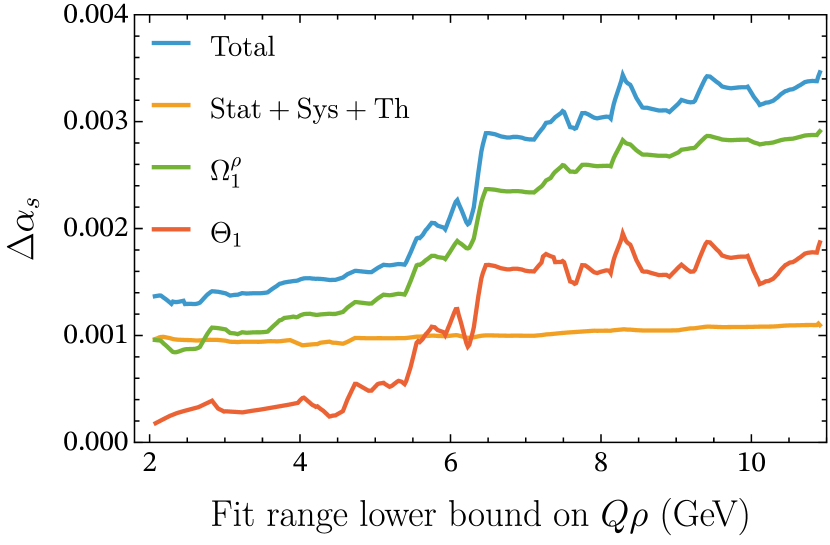
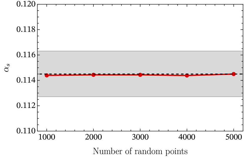
Figure 5: Left panel: Contributions to the total uncertainty as a function of the lower bound on the fit range for the full theory prediction (dijet + shoulder + $\Omega_{1}^{\rho}$ + $\Theta_{1}$). Right panel: In red we show the dependence of the best-fit value for $\alpha_{s}$ on the number of random profiles included in the scan in our best-fit setup, with the fit range $6\,{\rm GeV}/Q\leq\rho\leq 0.3$. The black dashed line and gray band correspond to the best-fit value and uncertainty with all 5000 profiles combined.

Uncertainty decomposition: The overall uncertainty on our final value for the strong coupling consists of three distinct parts: First, the combined experimental and perturbative theoretical uncertainties, where the former contains both statistical and systematic contributions. Second, the uncertainty induced by varying $\Omega_{1}^{\rho}$, and third, the uncertainty induced by varying $\Theta_{1}$. The contributions of these to the total uncertainties, as a function of the lower bound of the fit range, is displayed in the left panel of Fig. 5. When including more smaller-$\rho$ data, the fit uncertainty (yellow curve) is similar in size to the uncertainty induced by $\Omega_{1}^{\rho}$ (green curve), whereas the uncertainty arising from $\Theta_{1}$ (red curve) is comparatively small. This follows since, in most of the fit region, non-perturbative corrections mainly come from $\Omega_{1}^{\rho}$. Conversely, if cutting at higher values of $a/Q$, one expects an increasing contribution of $\Theta_{1}$ to the uncertainty budget, as the non-perturbative corrections arising from $\Theta_{1}$ become more important. This behavior is evident in the left panel of Fig. 5. In addition, we observe an almost linear rise of the uncertainty tied to $\Omega_{1}^{\rho}$ when increasing the lower bound of the fit range, which simultaneously yields a linear rise for the overall uncertainty on the strong coupling. Interestingly, the contribution from the fit uncertainty is rather flat, which suggests that the increased experimental uncertainty, due to less available data, is compensated for by a decrease of the perturbative theory uncertainty.

Random scans: In the right panel of Fig. 5 we show (in red) the fit result for the strong coupling as a function of the number of points used in the flat random scan. The fluctuation of the $\alpha_{s}$ central values stays well within our final fit uncertainty, displayed as the gray horizontal band. In general, we find that at least 3000 points are needed to reliably saturate the $n$-dimensional parameter space. In all our analyses we took the conservative approach of using 5000 points for the random scan, suppressing fluctuations in this regard and obtaining robust results throughout. Many ways of incorporating correlations among theory parameters have been proposed (see [47, 48, 49, 50, 51, 52, 53] and references therein) but the flat random scan offers the benefit of being both easy to implement and robust.

Figure 6: Convergence order-by-order in perturbation theory for FO (2D), FO+dij (2D) and FO+dij+sh (3D) and fixed values of the fit parameters. LO, NLO and NNLO denote the $\mathcal{O}(\alpha_{s})$, $\mathcal{O}(\alpha_{s}^{2})$ and $\mathcal{O}(\alpha_{s}^{3})$ FO predictions, respectively.

Convergence: In Fig. 6 we show HJM theory predictions for various levels of sophistication at different orders in perturbation theory, including scale variations. The left panel displays the fixed-order distribution, and the central panel includes dijet resummation. The latter yields substantially better convergent behavior. Note, however, that in the central panel near $\rho\approx 0.25$ there is visibly less overlap between the different orders. This behavior is to a large extent remedied when including shoulder resummation, as shown in the right panel. This demonstrates the convergent character of our best theory description, which includes dijet and shoulder resummation.

Order-by-order convergence of the cross section is expected to translate into order-by-order convergent fit results. Table 2 shows the difference between fits using the R-gap and $\overline{\rm MS}$ definitions for $\Omega_{1}$ at different orders in perturbation theory. Since this is a question associated with the dijet factorization we carry out fits for the simpler setup of the 2D fits using FO+dijet resummation. We see that the convergence in the two schemes is similar, while a slightly reduced fit uncertainty for $\alpha_{s}(m_{Z})$ is achieved in the R-gap scheme. This can be contrasted with the case of thrust [35, 36], where the reduction in uncertainty from the R-gap scheme was more significant.

	R-gap scheme			$\overline{\textrm{MS}}$ scheme
Order	$\alpha_{s}(m_{Z})$	$\Omega_{1}^{\rho}\,$[GeV]	$\chi^{2}/{\rm dof}$	$\alpha_{s}(m_{Z})$	$\bar{\Omega}_{1}^{\rho}\,$[GeV]	$\chi^{2}/{\rm dof}~$
N3LL′	$0.1137\pm 0.0016$	$0.59\pm 0.09$	$0.94$	$0.1154\pm 0.0020$	$0.50\pm 0.10$	$0.93$
N2LL′	$0.1166\pm 0.0027$	$0.52\pm 0.16$	$0.94$	$0.1178\pm 0.0031$	$0.49\pm 0.16$	$0.93$
NLL′	$0.1157\pm 0.0028$	$0.85\pm 0.12$	$0.98$	$0.1157\pm 0.0030$	$0.96\pm 0.10$	$0.99$

Table 2: Results of our 2D FO+dijet fits to the strong coupling and the leading power correction, both in the R-gap and $\overline{\textrm{MS}}$ schemes. The last three rows show the results for N³LL^′ + $\mathcal{O}(\alpha_{s}^{3})$, N²LL^′ + $\mathcal{O}(\alpha_{s}^{2})$, and NLL^′ + $\mathcal{O}(\alpha_{s})$ accuracy, respectively. Each determination is obtained from a fit to the dataset $\rho\in[4\,{\rm GeV}/Q,0.2]$. For each of the fit parameters at every order and scheme we display the central value and the fit uncertainty.

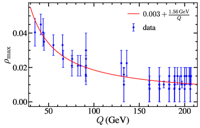
Figure 7: Location of peaks among the 50 available datasets (blue points), where the error bars show the bin size of the highest point in the differential cross section. These are well reproduced by the red curve given by $\rho_{\text{peak}}=0.003+1.56\,{\rm GeV}/Q$.

Peak region: For the lower bound of our fit range we use $a/Q$, in agreement with the argument from Ref. [35] for thrust that the peak position and increased sensitivity to non-perturbative effects goes as $1/Q$. That the peak position for HJM also goes as $1/Q$ is shown in Fig. 7, which displays the peak locations for for $50$ different datasets, represented by the blue dots. The error bars indicate the bin size of the highest point in the differential distribution for the given center-of-mass energy. The red curve corresponds to the function $\rho_{\text{peak}}=0.003+1.56\,{\rm GeV}/Q$. Our choice for the lower bound on the fit range, $a/Q$, is always taken to be well above these values.

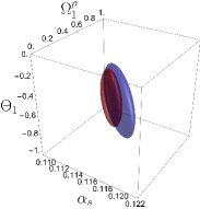
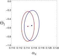
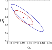
Figure 8: Correlations among the fit parmaters $\alpha_{s}$, $\Omega_{1}^{\rho}$ and $\Theta_{1}$. Ellipses are 1-$\sigma$ confidence intervals ($\Delta\chi^{2}=3.53$) shown for the fit range $Q\rho>3a_{\text{peak}}$ (red) and $Q\rho>6a_{\text{peak}}$ (blue).

Correlation among fit parameters: Fig. 8 displays the correlations among fit parameters for our best fit setup. The left panel shows the correlation among $\alpha_{s}$, $\Omega_{1}^{\rho}$ and $\Theta_{1}$ as an ellipsoid, whereas the remaining panels display its 2-dimensional orthographic projections. In particular, the second panel gives the correlation between $\Theta_{1}$ and $\Omega_{1}^{\rho}$, the third panel between $\Theta_{1}$ and $\alpha_{s}$, and the final panel between $\Omega_{1}^{\rho}$ and $\alpha_{s}$. The strongest correlation is between $\Omega_{1}^{\rho}$ and $\alpha_{s}$, which is also reflected in the fit result shown in Eq. (A Precise Determination of $\alpha_{s}$ from the Heavy Jet Mass Distribution), where the largest contribution to the overall uncertainty of $\alpha_{s}$ comes from the uncertainty induced by $\Omega_{1}^{\rho}$.

Fit components: The breakdown in uncertainties for the fits in Fig. 3 is given in Table 3. For fixed order, the lower bound of the fit range is varied from ${5a_{\text{peak}}}/{Q}$ to ${8a_{\text{peak}}}/{Q}$ while for the other fits it is varied from ${3a_{\text{peak}}}/{Q}$ to ${6a_{\text{peak}}}/{Q}$. Increasing the lower bound reduces the fit-range error for FO, but leads to a larger error from the NP parameter $\Omega_{1}^{\rho}$. With resummation, there is little sensitivity to the lower bound so it can be taken low, reducing the uncertainty from $\Omega_{1}^{\rho}$. If the lower bound is taken too close to $a_{\text{peak}}/Q$, higher order dijet power corrections of ${\cal O}(\Lambda^{2}_{\rm QCD})$ and beyond become leading order, necessitating a full non-perturbative shape function, so we always keep it above $3a_{\text{peak}}/Q$.

Model	$\alpha_{s}(m_{Z})$	th+exp	$\Omega_{1}^{\rho}$	$\Theta_{1}$	fit range	$\chi^{2}$/dof	$\Omega_{1}^{\rho}$ [GeV]	$\Theta_{1}$ [GeV]
Fixed Order 2D	$0.1166\pm 0.0034$	$\pm\,0.0014$	$\pm\,0.0027$	–	$\pm\,0.0015$	$1.108$	$0.06\pm 0.13$	–
FO + dijet 2D	$0.1148\pm 0.0018$	$\pm\,0.0010$	$\pm\,0.0014$	–	$\pm\,0.0004$	$1.055$	$0.53\pm 0.09$	–
FO + dijet 3D	$0.1156\pm 0.0024$	$\pm\,0.0010$	$\pm\,0.0021$	$\pm\,0.0004$	$\pm\,0.0007$	$1.052$	$\,0.52\pm 0.08\,$	$~\,\,0.53\pm 0.13$
FO + dijet + shoulder 3D	$0.1145\pm 0.0020$	$\pm\,0.0009$	$\pm\,0.0018$	$\pm\,0.0001$	$\pm\,0.0003$	$1.043$	$0.57\pm 0.09$	$-0.50\pm 0.17$

Table 3: Fits for $\alpha_{s},\Omega_{1}^{\rho}$ and $\Theta_{1}$ for different levels of theoretical sophistication. These numbers come from a weighted average of different fit-range lower bounds as described in the main text. The lower bound is taken as $c\,a_{\text{peak}}/Q$ with $c=5-8$ in steps of $0.5$ for FO 2D, and $c=3-6$ in steps of $0.5$ for the other three rows. (If FO 2D is taken with the same range as the other approximations, then its fit range uncertainty is even larger.)

References

- Salam and Wicke [2001] G. P. Salam and D. Wicke, Hadron masses and power corrections to event shapes, JHEP 05, 061, arXiv:hep-ph/0102343 .
- Movilla Fernandez et al. [2001] P. A. Movilla Fernandez, S. Bethke, O. Biebel, and S. Kluth, Tests of power corrections for event shapes in annihilation, Eur. Phys. J. C22, 1 (2001), arXiv:hep-ex/0105059 [hep-ex] .
- Gardi and Rathsman [2002] E. Gardi and J. Rathsman, The thrust and heavy-jet mass distributions in the two-jet region, Nucl. Phys. B638, 243 (2002), arXiv:hep-ph/0201019 .
- Dinsdale and Maxwell [2005] M. J. Dinsdale and C. J. Maxwell, Resummation of large logarithms within the method of effective charges, Nucl. Phys. B 713, 465 (2005), arXiv:hep-ph/0412118 .
- Becher and Schwartz [2008] T. Becher and M. D. Schwartz, A precise determination of from LEP thrust data using effective field theory, JHEP 07, 034, arXiv:0803.0342 [hep-ph] .
- Dissertori et al. [2009] G. Dissertori et al., Determination of the strong coupling constant using matched NNLO+NLLA predictions for hadronic event shapes in annihilations, JHEP 08, 036, arXiv:0906.3436 [hep-ph] .
- Chien and Schwartz [2010] Y.-T. Chien and M. D. Schwartz, Resummation of heavy jet mass and comparison to LEP data, JHEP 08, 058, arXiv:1005.1644 [hep-ph] .
- Alioli et al. [2013] S. Alioli, C. W. Bauer, C. J. Berggren, A. Hornig, F. J. Tackmann, et al., Combining Higher-Order Resummation with Multiple NLO Calculations and Parton Showers in GENEVA, JHEP 1309, 120, arXiv:1211.7049 [hep-ph] .
- Banfi et al. [2023] A. Banfi, B. K. El-Menoufi, and R. Wood, Interplay between perturbative and non-perturbative effects with the ARES method, JHEP 08, 221, arXiv:2303.01534 [hep-ph] .
- Navas et al. [2024] S. Navas et al. (Particle Data Group), Review of particle physics, Phys. Rev. D 110, 030001 (2024).
- Bhattacharya et al. [2022] A. Bhattacharya, M. D. Schwartz, and X. Zhang, Sudakov shoulder resummation for thrust and heavy jet mass, Phys. Rev. D 106, 074011 (2022), arXiv:2205.05702 [hep-ph] .
- Bhattacharya et al. [2023] A. Bhattacharya, J. K. L. Michel, M. D. Schwartz, I. W. Stewart, and X. Zhang, NNLL resummation of Sudakov shoulder logarithms in the heavy jet mass distribution, JHEP 11, 080, arXiv:2306.08033 [hep-ph] .
- Luisoni et al. [2021] G. Luisoni, P. F. Monni, and G. P. Salam, -parameter hadronisation in the symmetric 3-jet limit and impact on fits, Eur. Phys. J. C 81, 158 (2021), arXiv:2012.00622 [hep-ph] .
- Caola et al. [2022a] F. Caola, S. Ferrario Ravasio, G. Limatola, K. Melnikov, and P. Nason, On linear power corrections in certain collider observables, JHEP 01, 093, arXiv:2108.08897 [hep-ph] .
- Caola et al. [2022b] F. Caola, S. Ferrario Ravasio, G. Limatola, K. Melnikov, P. Nason, and M. A. Ozcelik, Linear power corrections to shape variables in the three-jet region, JHEP 12, 062, arXiv:2204.02247 [hep-ph] .
- Nason and Zanderighi [2023] P. Nason and G. Zanderighi, Fits of s using power corrections in the three-jet region, JHEP 06, 058, arXiv:2301.03607 [hep-ph] .
- Nason and Zanderighi [2025] P. Nason and G. Zanderighi, Fits of from event-shapes in the three-jet region: extension to all energies (2025), arXiv:2501.18173 [hep-ph] .
- Hoang et al. [2025] A. H. Hoang, V. Mateu, M. Schwartz, and I. W. Stewart, Precision Hemisphere Masses with Power Corrections, to appear (2025).
- Heister et al. [2004] A. Heister et al. (ALEPH), Studies of QCD at centre-of-mass energies between GeV and GeV, Eur. Phys. J. C35, 457 (2004).
- Abreu et al. [1996] P. Abreu et al. (DELPHI), Tuning and test of fragmentation models based on identified particles and precision event shape data, Z. Phys. C73, 11 (1996).
- Abreu et al. [1999] P. Abreu et al. (DELPHI), Energy dependence of event shapes and of at LEP-2, Phys. Lett. B456, 322 (1999).
- Abdallah et al. [2003] J. Abdallah et al. (DELPHI), A study of the energy evolution of event shape distributions and their means with the DELPHI detector at LEP, Eur. Phys. J. C29, 285 (2003), arXiv:hep-ex/0307048 .
- Movilla Fernandez et al. [1998] P. A. Movilla Fernandez, O. Biebel, S. Bethke, S. Kluth, and P. Pfeifenschneider (JADE), A study of event shapes and determinations of using data of annihilations at GeV to 44 GeV, Eur. Phys. J. C1, 461 (1998), arXiv:hep-ex/9708034 .
- Adeva et al. [1992] B. Adeva et al. (L3), Studies of hadronic event structure and comparisons with QCD models at the resonance, Z. Phys. C55, 39 (1992).
- Achard et al. [2004] P. Achard et al. (L3), Studies of hadronic event structure in annihilation from 30 GeV to 209 GeV with the L3 detector, Phys. Rept. 399, 71 (2004), arXiv:hep-ex/0406049 .
- Ackerstaff et al. [1997] K. Ackerstaff et al. (OPAL), QCD studies with annihilation data at 161 GeV, Z. Phys. C75, 193 (1997).
- Abbiendi et al. [2000] G. Abbiendi et al. (OPAL), QCD studies with annihilation data at 172 GeV to 189 GeV, Eur. Phys. J. C16, 185 (2000), arXiv:hep-ex/0002012 .
- Abbiendi et al. [2005] G. Abbiendi et al. (OPAL), Measurement of event shape distributions and moments in hadrons at 91 GeV – 209 GeV and a determination of , Eur. Phys. J. C40, 287 (2005), arXiv:hep-ex/0503051 .
- Abe et al. [1995] K. Abe et al. (SLD), Measurement of from hadronic event observables at the resonance, Phys. Rev. D51, 962 (1995), arXiv:hep-ex/9501003 .
- Catani et al. [1991] S. Catani, G. Turnock, and B. Webber, Heavy jet mass distribution in annihilation, Phys.Lett. B272, 368 (1991).
- Korchemsky and Sterman [1999] G. P. Korchemsky and G. Sterman, Power corrections to event shapes and factorization, Nucl. Phys. B555, 335 (1999), arXiv:hep-ph/9902341 .
- Fleming et al. [2008a] S. Fleming, A. H. Hoang, S. Mantry, and I. W. Stewart, Jets from massive unstable particles: Top-mass determination, Phys. Rev. D77, 074010 (2008a), arXiv:hep-ph/0703207 .
- Fleming et al. [2008b] S. Fleming, A. H. Hoang, S. Mantry, and I. W. Stewart, Top Jets in the Peak Region: Factorization Analysis with NLL Resummation, Phys. Rev. D77, 114003 (2008b), arXiv:0711.2079 [hep-ph] .
- Schwartz [2008] M. D. Schwartz, Resummation and NLO Matching of Event Shapes with Effective Field Theory, Phys. Rev. D77, 014026 (2008), arXiv:0709.2709 [hep-ph] .
- Abbate et al. [2011] R. Abbate, M. Fickinger, A. H. Hoang, V. Mateu, and I. W. Stewart, Thrust at N3LL with Power Corrections and a Precision Global Fit for , Phys. Rev. D83, 074021 (2011), arXiv:1006.3080 .
- Benitez et al. [2024] M. A. Benitez, A. H. Hoang, V. Mateu, I. W. Stewart, and G. Vita, On Determining from Dijets in Thrust (2024), arXiv:2412.15164 [hep-ph] .
- Catani and Seymour [1996] S. Catani and M. H. Seymour, The Dipole Formalism for the Calculation of QCD Jet Cross Sections at Next-to-Leading Order, Phys. Lett. B378, 287 (1996), arXiv:hep-ph/9602277 .
- Catani and Seymour [1997] S. Catani and M. H. Seymour, A general algorithm for calculating jet cross sections in NLO QCD, Nucl. Phys. B485, 291 (1997), arXiv:hep-ph/9605323 .
- Del Duca et al. [2016a] V. Del Duca, C. Duhr, A. Kardos, G. Somogyi, and Z. Trócsányi, Three-Jet Production in Electron-Positron Collisions at Next-to-Next-to-Leading Order Accuracy, Phys. Rev. Lett. 117, 152004 (2016a), arXiv:1603.08927 [hep-ph] .
- Del Duca et al. [2016b] V. Del Duca, C. Duhr, A. Kardos, G. Somogyi, Z. Szőr, Z. Trócsányi, and Z. Tulipánt, Jet production in the CoLoRFulNNLO method: event shapes in electron-positron collisions, Phys. Rev. D94, 074019 (2016b), arXiv:1606.03453 [hep-ph] .
- Hoang et al. [2015a] A. H. Hoang, D. W. Kolodrubetz, V. Mateu, and I. W. Stewart, -parameter distribution at N3LL′ including power corrections, Phys. Rev. D91, 094017 (2015a), arXiv:1411.6633 [hep-ph] .
- Dissertori et al. [2008] G. Dissertori et al., First determination of the strong coupling constant using NNLO predictions for hadronic event shapes in annihilations, JHEP 02, 040, arXiv:0712.0327 [hep-ph] .
- Mateu et al. [2013] V. Mateu, I. W. Stewart, and J. Thaler, Power Corrections to Event Shapes with Mass-Dependent Operators, Phys. Rev. D87, 014025 (2013), arXiv:1209.3781 [hep-ph] .
- Abbate et al. [2012] R. Abbate, M. Fickinger, A. H. Hoang, V. Mateu, and I. W. Stewart, Precision Thrust Cumulant Moments at N3LL, Phys. Rev. D86, 094002 (2012), arXiv:1204.5746 [hep-ph] .
- Wicke [1999] D. Wicke, Energy dependence of the event shape observables and the strong coupling. (In German) (1999), wU-B-DIS-1999-05.
- Hoang et al. [2015b] A. H. Hoang, D. W. Kolodrubetz, V. Mateu, and I. W. Stewart, Precise determination of from the -parameter distribution, Phys. Rev. D91, 094018 (2015b), arXiv:1501.04111 [hep-ph] .
- Cacciari and Houdeau [2011] M. Cacciari and N. Houdeau, Meaningful characterisation of perturbative theoretical uncertainties, JHEP 09, 039, arXiv:1105.5152 [hep-ph] .
- Becher et al. [2012] T. Becher, C. Lorentzen, and M. D. Schwartz, Resummation for and production at large , Phys. Rev. Lett. 108, 012001 (2012), arXiv:1106.4310 [hep-ph] .
- David and Passarino [2013] A. David and G. Passarino, How well can we guess theoretical uncertainties?, Phys. Lett. B 726, 266 (2013), arXiv:1307.1843 [hep-ph] .
- Bagnaschi et al. [2015] E. Bagnaschi, M. Cacciari, A. Guffanti, and L. Jenniches, An extensive survey of the estimation of uncertainties from missing higher orders in perturbative calculations, JHEP 02, 133, arXiv:1409.5036 [hep-ph] .
- Bonvini [2020] M. Bonvini, Probabilistic definition of the perturbative theoretical uncertainty from missing higher orders, Eur. Phys. J. C 80, 989 (2020), arXiv:2006.16293 [hep-ph] .
- Duhr et al. [2021] C. Duhr, A. Huss, A. Mazeliauskas, and R. Szafron, An analysis of Bayesian estimates for missing higher orders in perturbative calculations, JHEP 09, 122, arXiv:2106.04585 [hep-ph] .
- Tackmann [2024] F. J. Tackmann, Beyond Scale Variations: Perturbative Theory Uncertainties from Nuisance Parameters (2024), arXiv:2411.18606 [hep-ph] .