Many-body and QED effects in electron-atom inelastic scattering in EELS

Abstract

The elemental composition and electronic structure analysis of materials in Electron Energy Loss Spectroscopy (EELS) is probed by the inner shell ionization of atoms. This is a localized process in the material which can be well approximated by the scattering of a beam electron from a free atom. The inelastic differential cross section is calculated in the context of Quantum Electrodynamics (QED). The interaction of the incoming electron with the atom factorizes and it is treated perturbatively in QED. The atomic transition currents are calculated in the context of the relaxed Dirac-Hartree-Fock method. Correlation effects, which are induced by the relaxation of the atomic orbitals due to the created core-hole, are analyzed. Such effects are particularly important for quantum many-body systems and they are shown to have important impact on the shape of the differential cross section near the ionization threshold in Electron Energy Loss Spectra. In addition to the ionization spectrum, we calculate the excitation spectrum of Sc and Dy oxides using the crystal field multiplet theory. The calculation is compared to experimental EELS data and shows good agreement.

I Introduction

Inelastic scattering of fast charged particles with heavy targets has been the primary process to study the structure of matter at different energy scales. Atomic structure has been probed by electron-atom scattering experiments. Other examples include deep inelastic scattering experiments of electrons with nuclei and protons, which led to the discovery of quarks, [1].

The electron-matter interaction is still of great importance for the study of electronic structure of materials. Transmission Electron Microscopy (TEM) is a technique of high spatial resolution which reveals information about the elemental composition of materials through ionization processes and detection of the Energy Dispersive X-ray (EDS) and Electron Energy Loss Spectra (EELS). The EEL spectra are high-energy resolution and contain detailed information about the electronic structure of the material.

The primary electron energy in TEM is usually within the relativistic realm. Either a single atom in the material or the whole lattice is a heavy system compared to the free-beam electrons. Hence, its excitations can be described by an electromagnetic current operator which is minimally coupled to the beam electrons. The interaction between the two systems is weak and can be treated perturbatively as a series in $\alpha=e^{2}/\hbar c$. In the current work, we analyze the differential ionization cross section of a generic target which is excited or ionized by fast primary electrons within the natural framework of Quantum Field Theory. The differential cross section is calculated at tree level for any momentum transfer, such that $\alpha\mathbf{q}^{2}/m^{2}\ll 1$, where $m$ is the electron mass in natural units. The transition matrix, which appears in the cross section, factorizes to the perturbative part of the high energy electrons and the target transition current. The transition 4-current is expanded in a series of multipole operators, according to their transformation properties under $SO(3)$ symmetry. The QED differential ionization cross section is fully determined as a function of energy loss and momentum transfer taking into account the contributions from all the transverse degrees of freedom. The analytical expression of the QED differential cross section for a relativistic target is calculated in terms of the reduced matrix elements of the multipole components of the transition current between the angular momentum eigenstates of the system. The reduced matrix elements are simple one-dimensional integrals of the radial wavefunctions and can be used to calculate the excitation or ionization spectrum of any target. This expression can be applied to study different properties of the target such as the charge density and spin magnetic moments, [2]. There have been several calculations of the differential cross section for EELS, in the context of Quantum Mechanics, [3, 4], which were later extended by a semi-classical relativistic approximation of the electron-target interaction, [5]. Similar approaches consider the projection of the transition current on the beam direction since it is the main contribution for low momentum transfer, [6, 7, 8]. In another approach the Breit correction was added to the Coulomb interaction of the beam with the target which is the first term in the expansion of the scattering matrix in $v_{i}/c$, where $v_{i}$ is the velocity of the beam electrons, [9]. The total ionization cross section of K and L shell electrons in a relativistic framework, using the simplified atomic structure calculation based on the central Hartree-Slater mean field electron potential, is reported in [10]. The first term of the series expansion of our general result for low momentum transfer and energy loss agrees with the previous effective results.

The elemental composition of materials from EELS data does not require necessarily detailed knowledge of the embedding of the atom in the material. The calculation of the ionization of a core shell in the limit of a free static atom is applied to model the continuous part of the EEL spectrum. The transition currents are then calculated for free atoms, where the core shells are ionized with the emission of an electron to the continuum. We calculate the atomic transition currents in the microscopic framework of the relaxed Dirac-Hartree-Fock method, [11, 12, 13]. Further correlation effects in atoms can be included either by high accuracy methods such as configuration interaction, many-body perturbation theory, coupled cluster method, multi-configuration interaction or a combination of those, [14, 15, 16].

In the case of ionization experiments the correlation effects are important as was first discussed in photo-ionization processes, [13]. Those have been addressed by considering the relaxation of the atomic system in the final state due to the core-hole. This has been shown in plethora of atomic physics literature, [12, 13, 17, 18, 19], in X-ray absorption (XAS) spectroscopy and in EELS, [20, 21, 22, 23, 24, 25, 26, 27]. Such correlation effects are not explicitly included in ionization cross section calculations for EELS, where the atomic state is taken frozen and the core-hole is not included in the effective potential of the ionized electron. The asymptotic form of the one particle mean field potential is typically adjusted to match the expected large distance behavior, [3, 4, 10, 28]. In other cases, such effects are approximated by effective one particle Density Functional Theory (DFT) potentials, [29]. Single particle potentials for correlation effects of inner atomic shells are only approximated by considering semi-local information in the density functionals, [30].

However, the relaxation of finite quantum systems due to the core-hole can be described explicitly from first principles using many-body theory and the random phase approximation which reduce to the delta-self-consistent-field calculation, [31, 32, 33, 34, 35, 36]. For exciations which are not localized in solid state systems, the electron-hole interaction should be taken into account within many body perturbation theory and methods such GW and Bethe-Salpeter equation in order to achieve reasonable agreement with the experiment, [37, 36, 38].

The core-hole is well separated in energy from the excited states of the atom. As a result, the treatment in random phase approximation is shown to be equivalent to the self-consistent Dirac-Hartree-Fock solution of the ionized atom with a core-hole present and an outgoing ionized electron, where the atomic orbitals are rearranged due to the hole, [39]. This has been shown to have a significant influence on the ionization energies,[40], and on the spectral shapes in ionization data of atoms, especially for core shell electrons, [17, 41]. We explicitly include the core-hole in the final state of the scattering process from a microscopic point of view without an effective potential. We particularly show this effect, especially in the shape of delayed edges such as the $3\text{d}$. The interaction of the core-hole with the excited electrons in discrete states also plays a crucial role in the description of excitation spectra of transition metal oxides, [42]. This approach addresses the main correlation effects in atomic transitions which involve core shells. Additional dynamic effects due to the decay of the core-hole can also be included in the current scheme, [41].

An important aspect of EELS experiments is the study of the excitation part of the spectra of transition metal and rare earth elements, [26]. This has an excitonic behavior which reveals important information about the oxidation state of the elements and the electronic structure of the valence shells which controls the magnetic properties of the material. In the current work, we calculate the excitation and ionization differential cross section of Sc and Dy using the atomic multiplet theory, [43, 42]. The interaction of the core-hole with the excited electrons contributes significantly to the spectral shape.

The structure of the current paper is as follows, in section II, we derive the general expression of the inelastic differential cross section of an electron with a spherically symmetric heavy target in terms of the reduced matrix elements of the transition current of the target. In section III, the reduced transition current is calculated for a relativistic target which is described by a many particle state in the basis of Dirac orbital wavefunctions. The low momentum transfer limit is found and it is shown to correspond to previous results and higher order terms are included. Finally, in section IV some details on the numerical calculation and results of the differential cross section for several atoms is given. The total excitation and ionization spectrum of Sc and Dy in $\textrm{DyScO}_{3}$ is calculated and compared to its experimental EEL Spectrum. Initial results of the many body effects on inner shell ionization have been reported in [44].

II Inelastic electron scattering

II.1 Quantum Electrodynamics

The beam electron interaction with a heavy target is described by coupling an external electromagnetic current operator $\mathcal{J}^{\mu}(x)=(\rho(x),{\mathbf{\mathcal{J}}}(x))$ to the QED Lagrangian

$${\cal L}=-\frac{1}{4}F^{\mu\nu}F_{\mu\nu}-\overline{\Psi}\left([\not{\partial}+ie\not{A}]+m\right)\Psi+\mathcal{J}^{\mu}A_{\mu}\,,$$ (1)

where $A_{\mu}$ is the photon field, $F_{\mu\nu}=\partial_{\mu}A_{\nu}-\partial_{n}A_{\mu}$, $\Psi$ is the electron spinor field. The standard notation is adopted, $\not{S}=\gamma^{\mu}S_{\mu}$ and $\partial_{\mu}=\frac{\partial}{\partial x_{\mu}}$. The metric convention is mostly plus, $\eta_{\mu\nu}=\textrm{diag}(-1,1,1,1)$ and the gamma matrices follow the Weyl notation. The external electromagnetic current operator is conserved, $\partial_{\mu}{\mathcal{J}}^{\mu}(x)=0$. We adopt the natural units, where $\hbar=c=1$.

The inelastic scattering for high energy electrons is then described at tree level by the Feynman diagram in Fig. (1).

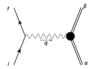
Figure 1: Tree level diagram for the inelastic scattering of an incoming electron ($i\to f$) by a heavy target which is excited from state $\alpha$ to $\beta$. In our case $\beta$ will be either an ionized or and excited state.

The Feynman rules from the Lagrangian (1) imply for the S-matrix for the scattering process in momentum space

$$S_{p_{f},m_{s_{f}},\,\beta\,;\,p_{i},m_{s_{i}},\,\alpha} =\langle p_{f},s_{f},\,\beta|S|p_{i},s_{i},\,\alpha\rangle$$

$$=-\frac{e}{(2\pi)^{3}}\delta(E_{f}-E_{i}-E_{\alpha}+E_{\beta})\frac{\bar{u}(p_{f},m_{s_{f}})\gamma_{\mu}u(p_{i},m_{s_{i}})}{q^{2}}\langle\beta|\mathcal{J}_{\mu}(\mathbf{q})|\alpha\rangle\,,$$ (2)

where $q=p_{i}-p_{f}$ are all 4-vectors, i.e. $q=(E_{i}-E_{f},{\bf p_{i}}-{\bf p_{f}})$. Time translation symmetry leads to a transition current of the form $\mathcal{J}^{\mu}(q)=e^{i(E_{\beta}-E_{\alpha})t}\int d^{3}xe^{-i{\bf q\cdot x}}\mathcal{J}^{\mu}({\bf x})=e^{i(E_{\beta}-E_{\alpha})t}\mathcal{J}^{\mu}(\mathbf{q})$. By factoring out the energy conserving delta function one can retrieve the transition matrix which is defined as

$$S_{p_{f},s_{f},\,\beta\,;\,p_{i},s_{i},\,\alpha}=\delta(\{f,\beta\}-\{i,\alpha\})-2\pi\,i\delta(E_{f}-E_{i}+E_{\beta}-E_{\alpha})T_{p_{f},s_{f},\,\beta\,;\,p_{i},s_{i},\,\alpha}.$$ (3)

Considering an unpolarized electron beam and the fact that the spin of the beam electrons is not measured in an EELS detector, we average and sum over the initial and final spin states respectively. The norm of the t-matrix is

$$|T_{p_{f},\,\beta\,;\,p_{i},\,\alpha}|^{2}=-\frac{e^{2}}{2q^{4}}\frac{1}{E_{i}E_{f}}\left((p_{i}\cdot p_{f}+m^{2})\eta^{\mu\nu}-p_{i}^{\mu}\,p_{f}^{\nu}-p_{i}^{\nu}\,p_{f}^{\mu}\right)\langle\beta|\mathcal{J}_{\mu}(\mathbf{q})|\alpha\rangle\,\langle\beta|\mathcal{J}_{\nu}^{\dagger}(\mathbf{q})|\alpha\rangle$$ (4)

where the beam electron contribution factorizes from the transition current of the target. This is a very generic fact which is well known from similar particle physics processes.

Finally, the inelastic differential cross section of an unpolarized incoming electron beam interacting with a heavy target reads

$$\sigma(p_{f},\,\beta\,;\,p_{i},\,\alpha)=(2\pi)^{4}\frac{1}{|\mathbf{v}_{i}|}\,\sum_{\beta}\int d\beta\,\delta(E_{f}-E_{i}+E_{\beta}-E_{\alpha})\,|T_{p_{f},\,\beta\,;\,p_{i},\,\alpha}|^{2}\,,$$ (5)

where we sum and integrate over the discrete and continuous quantum numbers of the final state $\beta$. ${\bf v}_{i}$ is the velocity of the incoming electrons.

II.2 Multipole expansion of the T-matrix

The non trivial part of the diagram in (1) is the right vertex which includes the target transition matrix element and contains the information about the target excitations. We now consider that the target spectrum consists of angular-momentum eigenstates, so $J_{\alpha}^{2}|\alpha\rangle=J_{\alpha}(J_{\alpha}+1)|\alpha\rangle$. In this case, we will expand the current matrix element to $SO(3)$ irreducible tensor operators.

We choose the z axis of our coordinate system along the virtual photon momentum $\mathbf{q}$, without loss of generality for an unpolarized sample, [2]. One can consider, rotating the quantization axis to an arbitrary direction without any impact to the final cross section.

The conservation of the 4-current as expressed in terms of the charge density and the transverse vector transition current

$$\hat{e}_{(\mathbf{q})}\cdot{\bm{\mathcal{J}}}(\mathbf{q})=\frac{q_{0}}{|\mathbf{q}|}\rho(\mathbf{q})\,.$$ (6)

Eq. (4) can then be written as

$$|T_{p_{f},\,\beta\,;\,p_{i},\,\alpha}|^{2}=-{e^{2}\over 2q^{4}}{1\over E_{i}E_{f}}\left(C_{L}(q)|\rho(\mathbf{q})|^{2}+C_{T}(q)|\bm{\mathcal{J}_{\perp}}(\mathbf{q})|^{2}\right)$$ (7)

The coefficients of the longitudinal and transverse terms are

$$C_{L}(q)={1\over 2}{q^{4}\over|\mathbf{q}|^{4}}\left[\left(E_{i}+E_{f}\right)^{2}-|\mathbf{q}|^{2}\right]$$

$$C_{T}(q)=|\mathbf{P}|^{2}-{\left(\mathbf{q}\cdot\mathbf{P}\right)^{2}\over|\mathbf{q}|^{2}}+{q^{2}\over 2}\,,$$ (8)

and ${\mathbf{P}}=\frac{\mathbf{p}_{i}+\mathbf{p}_{f}}{2}$. The charge and current densities in the coordinate space are

$$\rho(\mathbf{q})=\int d^{3}x\,e^{-i\mathbf{q}\cdot\mathbf{x}}\rho(\mathbf{x})\,,\,\,{\bm{\mathcal{J}}_{\perp}}(\mathbf{q})=\int d^{3}x\,e^{-i\mathbf{q}\cdot\mathbf{x}}{\bm{\mathcal{J}}_{\perp}}(\mathbf{x})$$ (9)

The plane wave expansion in terms of spherical harmonics is applied to the charge density

$$e^{-i\mathbf{q}\cdot\mathbf{x}}=\sqrt{4\pi}\sum_{J}(-i)^{J}\sqrt{2J+1}j_{J}(|\mathbf{q}|r)Y_{J}^{0}(\hat{\mathbf{x}})\,.$$ (10)

The vector current is expanded in terms of the spherical components of the $\hat{e}_{(\mathbf{q})}$ basis.

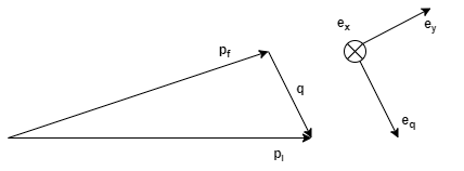
Figure 2: The coordinate system of the expansion of the vector current operator is defined with respect to the momentum transfer vector.

Then, the $\lambda$ spherical component of the current is $\mathcal{J}_{\lambda}=\hat{e}_{(\mathbf{q})\,\lambda}\cdot\mathcal{J}$. The spherical vector is coupled to the spherical harmonics from the plane wave expansion, Eq. (10),

$$\hat{e}_{(\mathbf{q})\,\lambda}e^{-i\mathbf{q}\cdot\mathbf{x}}= -\sqrt{2\pi}\sum_{J=1}^{\infty}(-i)^{J}\sqrt{2J+1}\Bigg{[}\lambda j_{J}(|\mathbf{q}|r)\mathbf{Y}_{JJ}^{\lambda}(\hat{\mathbf{x}})$$

$$\left.+i\left(\sqrt{J+1\over 2J+1}j_{J-1}\left(|\mathbf{q}||\mathbf{x}|\right)\mathbf{Y}_{J\,J-1}^{\lambda}(\hat{\mathbf{x}})-\sqrt{J\over 2J+1}j_{J+1}\left(|\mathbf{q}||\mathbf{x}|\right)\mathbf{Y}_{J\,J+1}^{\lambda}(\hat{\mathbf{x}})\right)\right]$$ (11)

The norm of the above expressions is calculated in terms of the irreducible matrix elements of the current operator

$${1\over 2J_{\alpha}+1}\sum_{M_{\alpha}\,M_{\beta}}|T_{p_{f},\,\beta\,;\,p_{i},\,\alpha}|^{2} ={e^{2}\over(2\pi)^{5}}{1\over q^{4}}{1\over E_{i}E_{f}}{1\over 2J_{\alpha}+1}\left[C_{L}(q)\,\sum_{J=0}^{\infty}\left|\langle\beta||T_{J}^{M\,\mathrm{(}coul)}||\alpha\rangle\right|^{2}\right.$$

$$\left.+C_{T}(q)\sum_{J=1}^{\infty}\left(\left|\langle\beta||T_{J}^{\mathrm{(}e)}||\alpha\rangle\right|^{2}+\left|\langle\beta||T_{J}^{\mathrm{(}m)}||\alpha\rangle\right|^{2}\right)\right]$$ (12)

where we average and sum over the initial and final projections of the angular momentum respectively. The irreducible parts of the current operator under $SO(3)$ in terms of the vector spherical harmonics are

$$T_{J}^{M\,\mathrm{(}coul)}= \int d^{3}\mathbf{x}\,j_{J}\left(|\mathbf{q}||\mathbf{x}|\right)Y_{J}^{M}(\hat{\mathbf{x}})\rho(\mathbf{x})$$

$$T_{J}^{M\,\mathrm{(}mag)}= \int d^{3}\mathbf{x}\,j_{J}(|\mathbf{q}||\mathbf{x}|)\mathbf{Y}_{JJ}^{M}(\hat{\mathbf{x}})\cdot{\bm{\mathcal{J}}}(\mathbf{x})$$ (13)

$$T_{J}^{M\,\mathrm{(}el)}= \int d^{3}\mathbf{x}\,\left[\sqrt{J+1\over 2J+1}j_{J-1}\left(|\mathbf{q}||\mathbf{x}|\right)\mathbf{Y}_{J\,J-1}^{M}(\hat{\mathbf{x}})\cdot{\bm{\mathcal{J}}}(\mathbf{x})\right.$$

$$\left.-\sqrt{J\over 2J+1}j_{J+1}\left(|\mathbf{q}||\mathbf{x}|\right)\mathbf{Y}_{J\,J+1}^{M}(\hat{\mathbf{x}})\cdot{\bm{\mathcal{J}}}(\mathbf{x})\right].$$

As a result, the most general expression for the inelastic scattering differential cross section can be written in terms of the reduced transition matrix elements of the irreducible current tensor operators

$${d^{2}\sigma\over d\Omega_{f}dE} ={e^{2}\over 2\pi}{p_{f}\over p_{i}}\,{1\over q^{4}}{1\over 2J_{\alpha}+1}\left[C_{L}(q)\,\sum_{J=0}^{\infty}\left|\langle\beta||T_{J}^{\mathrm{(}coul)}||\alpha\rangle\right|^{2}\right.$$

$$\left.+C_{T}(q)\sum_{J=1}^{\infty}\left(\left|\langle\beta||T_{J}^{\mathrm{(}el)}||\alpha\rangle\right|^{2}+\left|\langle\beta||T_{J}^{\mathrm{(}mag)}||\alpha\rangle\right|^{2}\right)\right]$$ (14)

II.2.1 Kinematics

In the lab frame of the collision, the kinematics are defined by the scattering angle, $\theta$, and the energy loss, $E$, of the incident electron to the target. It is common to exchange the $\theta$ to $|\mathbf{q}|$ variable. The momentum transfer is

$$|\mathbf{q}|^{2}=(|\mathbf{p}_{i}|-|\mathbf{p}_{f}|)^{2}(1+\tilde{\theta}^{2})\,,\,\,\tilde{\theta}^{2}=\frac{4|\mathbf{p}_{i}|\,|\mathbf{p}_{f}|}{(|\mathbf{p}_{i}|-|\mathbf{p}_{f}|)^{2}}\sin^{2}\frac{\theta}{2}\,,$$ (15)

where $\tilde{\theta}$ depends collection angle but scaled appropriately with the energy loss, $E$. For low $\theta$ and $E$ this expression reduces to the scaled angle which was defined in [5] for the investigation of relativistic effects in the cross section

$$\tilde{\theta}\simeq\frac{|\mathbf{p}_{i}|^{2}}{E_{i}^{2}}\frac{\theta}{\epsilon}$$ (16)

where $\epsilon=\frac{E}{E_{i}}$. In the lab frame, the longitudinal and transverse coefficients can be written as

$$C_{L}(q) ={1\over 2}\left(1-{E^{2}\over|\mathbf{q}|^{2}}\right)^{2}\left(4E_{i}^{2}-4E_{i}\,E+E^{2}-|\mathbf{q}|^{2}\right)$$

$$=\frac{1}{2}{\left(1-{|\mathbf{p}_{i}|^{2}\over E_{i}^{2}}+\tilde{\theta}^{2}\right)^{2}\over(1+\tilde{\theta}^{2})^{2}}\left[(2E_{i}-E)^{2}-(|\mathbf{p}_{i}|-|\mathbf{p}_{f}|)^{2}(1+\tilde{\theta}^{2})\right]$$ (17)

$$C_{T}(q) ={2|\mathbf{p}_{i}||\mathbf{p}_{f}|\,\sin^{2}{\theta\over 2}\over|\mathbf{q}|^{2}}\left[\left(|\mathbf{p}_{i}|+|\mathbf{p}_{f}|\right)^{2}-2|\mathbf{p}_{i}||\mathbf{p}_{f}|\,\cos^{2}{\theta\over 2}\right]+{(|\mathbf{p}_{i}|-|\mathbf{p}_{f}|)^{2}-E^{2}\over 2}$$

$$=\frac{(|\mathbf{p}_{i}|-|\mathbf{p}_{f}|)^{2}-E^{2}}{2}+{\tilde{\theta}^{2}\over 1+\tilde{\theta}^{2}}\left(p_{i}^{2}+p_{f}^{2}+{(|\mathbf{p}_{i}|-|\mathbf{p}_{f}|)^{2}\over 2}\tilde{\theta}^{2}\right)$$

It is noticed the transverse part becomes important for large scattering angle and energy loss. In case of experiments such as reflection EELS the outgoing electrons are detected at large scattering angle, so the transverse interaction with the target is probed. On the other hand, for low energy of the incident electrons the relativistic effects are small.

II.3 Photoionization

The ionization cross section of an atom by a high energy photon is relevant for X-ray Absorption Spectroscopy (XAS). EELS and XAS signals contain similar information about the samples and they are typically compared. The ionization cross section is given by a similar expression as (5), with the identification of the photon energy as the difference of the electron energy loss $E=E_{i}-E_{f}$. The transition matrix element is

$$|T_{\beta;\alpha,k}|^{2}=\frac{1}{4\pi E}|\mathcal{J}^{\mu}\,\varepsilon_{\mu}(k,\lambda)|^{2}\,.$$ (18)

$\varepsilon_{\mu}(k,\lambda)$ is the photon polarization vector and $E=k^{0}=|\bm{k}|$. We can consider here the $\bm{k}\cdot\bm{\varepsilon}(k,\lambda)=0$ and $\varepsilon^{0}(k,\lambda)=0$. Following the same steps as in section II.2 and summing over all the photon final polarizations, the multipole expansion gives

$$\sigma_{\gamma}(E)=(2\pi)^{4}{1\over 2J_{\alpha}+1}\sum_{M_{\alpha}\,M_{\beta}}|T_{\beta;\alpha,k}|^{2}=\frac{(2\pi)^{3}}{2E}{1\over 2J_{\alpha}+1}\sum_{J=1}^{\infty}\left(\left|\langle\beta||T_{J}^{\mathrm{(}el)}||\alpha\rangle\right|^{2}+\left|\langle\beta||T_{J}^{\mathrm{(}mag)}||\alpha\rangle\right|^{2}\right)$$ (19)

where the T-matrix elements are given by Eq. (13). The transverse parts of the two cross sections obviously have the same structure. We will later show that for low momentum transfer the leading term in $T^{(e)}$ is similar to the dipole approximation of $T^{(coul)}$. This is the reason why the XAS signal is similar to the EELS signal.

The multipole expansion, section (II.2), of the photon atom interaction is particularly interesting in inelastic X-ray scattering (IXS) experiments where contributions beyond dipole are important, [45]. The multipole expansion of the IXS cross section has been studied in [46], where the target Hamiltonian has been expanded to powers of $1/c$ .

III Atomic Structure

When inner atomic shells are excited the final state can include resonances and a continuous spectrum. In the current work, we are focusing on excitations to the continuum which is mainly used in the EELS data processing for the determination of the elemental composition of materials. In this case, the neighboring atoms modify the fine structure of the shape but not the overall trend. Detailed description of the edge fine structure typically requires a simulation of the lattice cell, [22, 24, 25]. We currently focus on the continuum part of the spectral function, so we consider the target of the scattering process to be an atom described by the current operator $\mathcal{J}$. The initial state is the ground state of the atom and the final state is an ion with an inner shell hole and an ejected electron.

III.1 The electromagnetic current for Dirac orbitals

The dynamics of a neutral atom of atomic number Z, with N electrons, is described by the QED Lagrangian, (1), with a static external nuclear current density ${\mathcal{J}^{\mu}_{nucl}}(\mathbf{x})=(\rho_{nucl}(\mathbf{x}),{\bf 0})$ assuming that the nucleus magnetic moment has a small effect. High-accuracy atomic structure calculations take into account the leading relativistic effects coming from the Dirac equation, [11], while higher-order QED effects have been considered for heavy atoms. For an elementary introduction of bound states in QED, see [47] and for the tree-level correction to the multi-electron atoms, see [48]. Those are explored in the current article for transitions with higher ionization energy.

The ansatz for the ground state wavefunction is taken to be a fully antisymmetric Slater determinant

$$|\Psi\rangle =|\psi_{1}\ldots\psi_{N}\rangle={1\over\sqrt{N!}}\sum_{P}(-1)^{P}|\psi_{P(1}\rangle\otimes|\psi_{P(2}\rangle\otimes\ldots\otimes|\psi_{P(N)}\rangle\,.$$ (20)

A linear combination of determinants is formed for multiple configurations, [49], [50]. The solution for the atomic ground states is described in detail in (III.3).

The matrix element of the electromagnetic current operator on N-particle fermion states can be expressed in terms of matrix elements of the one particle orbitals $|\psi_{i}\rangle$. The details of the derivation for general states is shown in the Appendix C.

The ansatz for the single particle orbitals is taken to be the central field Dirac spinors

$$\psi_{n}(\mathbf{x})=\begin{pmatrix}f_{n}(\mathbf{x})+i\,g_{n}(\mathbf{x})\\ f_{n}(\mathbf{x})-i\,g_{n}(\mathbf{x})\end{pmatrix}$$ (21)

where $f_{n}(\mathbf{x})=\Omega_{\kappa\,m}({\hat{\mathbf{x}}})F_{n}(r)$ and $g_{n}(\mathbf{x})=\Omega_{-\kappa\,m}({\hat{\mathbf{x}}})G_{n}(r)$

$$\Omega_{\kappa\,m}({\hat{\mathbf{x}}})=\begin{pmatrix}C_{j\mp{1\over 2}\,,{1\over 2}}(j,m\;m-{1\over 2},{1\over 2})Y^{m-{1\over 2}}_{j\mp{1\over 2}}\\ C_{j\mp{1\over 2}\,,{1\over 2}}(j,m\;m+{1\over 2},{1\over 2})Y^{m+{1\over 2}}_{j\mp{1\over 2}}\end{pmatrix}$$ (22)

and $\Omega_{-\kappa\,m}({\hat{\mathbf{x}}})=(\bm{\sigma}\cdot\mathbf{x})\,\Omega_{\kappa\,m}({\hat{\mathbf{x}}})$.

The current matrix element between two energy eigenstates is defined as

$$\mathcal{J}_{mn}^{\mu}(x)=\langle\psi_{m}|\mathcal{J}^{\mu}(x)|\psi_{n}\rangle=-ie\,e^{i(E_{m}-E_{n})t}\overline{\psi}_{m}(\mathbf{x})\gamma^{\mu}\psi_{n}(\mathbf{x})$$ (23)

The electromagnetic current components in terms of the wavefunction ansatz in (21)

$$\mathcal{J}_{mn}^{0}(\mathbf{x}) =-e\,\left(f_{m}^{\dagger}(\mathbf{x})f_{n}(\mathbf{x})+g_{m}^{\dagger}(\mathbf{x})g_{n}(\mathbf{x})\right)$$ (24)

$${\bm{\mathcal{J}}}_{mn}(\mathbf{x}) =ie\,\left(f_{m}^{\dagger}(\mathbf{x}){\bm{\sigma}}g_{n}(\mathbf{x})+g_{m}^{\dagger}(\mathbf{x}){\bm{\sigma}}f_{n}(\mathbf{x})\right)$$ (25)

Equations (13) lead to the T-matrix elements in terms of the radial Dirac wavefunctions. The calculation of the irreducible matrix elements of the current operator with the vector spherical spinors is shown in detail in Appendix (B). The final result reads

$$\langle m||T_{J}^{\mathrm{(}coul)}||n\rangle =-e\langle\kappa_{m}||Y_{J}(\hat{x})||\kappa_{n}\rangle\int dr\,r^{2}j_{J}\left(|\mathbf{q}|r\right)\left[F_{m}^{\dagger}(r)F_{n}(r)+G_{m}^{\dagger}(r)G_{n}(r)\right]$$

$$\langle m||T_{J}^{(mag)}||n\rangle =-i\,e{(\kappa_{n}+\kappa_{m})\over\sqrt{J(J+1)}}\langle\kappa_{m},||Y_{J}||-\kappa_{n}\rangle\int dr\,r^{2}\,j_{J}\left(|\mathbf{q}|r\right)\left(F_{m}^{\dagger}(r)G_{n}(r)+G_{m}^{\dagger}(r)F_{n}(r)\right)$$ (26)

$$\langle m||T_{J}^{(el)}||n\rangle =-i\,e\,\sqrt{J+1\over J}\langle\kappa_{m}||Y_{J}^{M}||\kappa_{n}\rangle\int dr\,r^{2}\,\left[{\kappa_{n}-\kappa_{m}\over J+1}\left({j_{J}\left(|\mathbf{q}|r\right)\over|\mathbf{q}|\,r}+j_{J}^{\prime}(|\mathbf{q}|\,r)\right)\right.$$

$$\left.\times\left(F_{m}^{\dagger}(r)G_{n}(r)+G_{m}^{\dagger}(r)F_{n}(r)\right)+J\,{j_{J}\left(|\mathbf{q}|r\right)\over|\mathbf{q}|\,r}\left(F_{m}^{\dagger}(r)G_{n}(r)-G_{m}^{\dagger}(r)F_{n}(r)\right)\right]$$

where the reduced matrix element of the spherical harmonic $Y_{J}$ is defined as

$$\langle\kappa_{m}||Y_{J}||\kappa_{n}\rangle={(-1)^{j_{m}-{1\over 2}}\over\sqrt{4\pi}}\,\left[j_{m},\,J,\,j_{n}\right]^{1\over 2}\begin{pmatrix}j_{m}&J&j_{n}\\ {1\over 2}&0&-{1\over 2}\end{pmatrix}$$ (27)

Those are the most general expressions for the T-matrix for the scattering of a relativistic electron in terms of the angular momentum eigenstates of relativistic bound electrons which are described by the Dirac equation. It is evident from those expressions that the nontrivial contributions by the Dirac solutions to the cross section stems from the mixing terms in the transverse matrix elements. Those are the one-particle expressions which are applied to the calculation of the matrix elements of the many-body state in terms of the one-particle orbital basis, see appendix (C). This result is directly applicable to configuration interaction states, which are expressed as linear combination of Slater determinants.

The expressions for $T^{(e)}$ and $T^{(m)}$ are essentially the same in the multipole expansion of the relativisic photoionization cross section and x-ray emission rate, Eq. (19), which has been derived in [11, 51, 52].

The exchange interaction of the beam electron with the target electrons is suppressed by $\sim 1/{p_{i}}$. As soon as the incoming electron has a much higher energy than the ionized one, the exchange interaction is heavily suppressed. When the incoming electron energy is low enough compared to the ionized electron kinetic energy the whole system should be solved self-consistently. At least one should add the exchange interaction to the beam-target potential, but this is relevant for low beam energies, [9]. This case can be treated non-relativistically and we do not focus on this in the current work.

III.2 The low momentum-transfer limit

Eqs.  (14) and (26) are the most general expression for the ionization cross section of a relativistic target by high energy electrons for any momentum transfer at tree level. The relevant energy scales in an EELS experiment are the beam energy, the momentum transfer and the energy loss, which is directly related with the target excitations which are probed. Typically, low momentum transfer and low energy loss experiments are performed in a TEM with a relativistic beam. As a result, the relativistic kinematics of the beam is necessary to be included in EELS analysis. The beam-target interaction then typically includes the Coulomb contribution and possibly the dipole part from the transverse part of the interaction, as the main relativistic correction to the cross section, [6], and later reproduced in [5], [8].

The atomic states can be described by Dirac or Schrodinger orbital wavefunctions. In the second case, the first-order relativistic effects, such as the spin-orbit interaction, are included perturbatively. The main difference between the relativistic and non-relativistic treatment of the target in the cross section is brought by the magnetic and electric matrix elements. We here derive the long-wavelength limit from the full cross section expression for a non-relativistic target. It is also important to notice that solving the Dirac equation for the target in a constant external potential does not give the complete relativistic picture for deep enough shells, since dynamical QED effects are not included. However, such contributions are too small for the most common energy range of EELS experiments. In this section, we show how the complete expression for the differential cross section reduces to the lowest order relativistic corrections and what are the next order terms of the expansion in the energy loss and scattering angle.

When the velocity of the bound electrons to the atom is non-relativistic, $\langle v\rangle/c\ll 1$, the orbital wave functions reduce to

$$G(r)\simeq-\frac{1}{2m}\left({dF(r)\over dr}+{\kappa+1\over r}F(r)\right)\,.$$ (28)

The expansion of the Coulomb matrix element $T^{(coul)}$ is already trivial, since the second term is second order in $G(r)$. Hence, there is no correction to first order. As a result, the Dirac equation will make a significant difference in electron-target interaction when transverse effects are included. Using Eq. (28), the magnetic part of the T-matrix becomes

$$\langle m||T_{J}^{(mag)}||n\rangle= \frac{i\,e}{2m}{(\kappa_{n}+\kappa_{m})\over\sqrt{J(J+1)}}\langle\kappa_{m}||Y_{J}||-\kappa_{n}\rangle\,$$

$$\times\int_{0}^{\infty}dr\left((\kappa_{n}+\kappa_{m})\,r\,j_{J}(|\mathbf{q}|r)-r^{2}{d\over dr}j_{J}(|\mathbf{q}|r)\right)F_{m}(r)F_{n}(r)$$ (29)

The ionized electron’s wavefunction is non-relativistic when the momentum transfer is small, $|\mathbf{q}|r\ll 1$, where $r$ is the characteristic radial distance where the continuum wavefunction overlaps with the core-hole shell. In this case, the spherical Bessel function can be expanded to

$$j_{J}(|\mathbf{q}|r)={(|\mathbf{q}|r)^{J}\over(2J+1)!!}\,.$$ (30)

With some algebra the long-wavelength approximation for the magnetic part reduces to

$$\langle m||T_{J}^{(mag)}||n\rangle= {i\,e\over 2m}{(\kappa_{n}+\kappa_{m})\left(\kappa_{n}+\kappa_{m}-J\right)\over(2J+1)!!\sqrt{J(J+1)}}\langle\kappa_{m},||Y_{J}||-\kappa_{n}\rangle\,|\mathbf{q}|^{J}$$

$$\times\int dr\,r^{J+1}F_{m}(r)F_{n}(r)\,.$$ (31)

The electric part leads to

$$\langle\beta||T_{J}^{(el)}||\alpha\rangle= {i\,e\over 2m}\,\sqrt{J+1\over J}\langle\kappa_{m}||Y_{J}||\kappa_{\alpha}\rangle\,{2J\over(2J+1)!!}|\mathbf{q}|^{J-1}$$

$$\times\int_{0}^{\infty}dr\,r^{J+1\over 2}F_{m}\left({d\over dr}+{(\kappa_{n}-\kappa_{m})(\kappa_{n}+\kappa_{m}+1)\over 2J\,r}\right)\left(r^{J+1\over 2}F_{n}\right)$$ (32)

This is an extension of the standard electric dipole ($J=1$) transition matrix element in the velocity gauge, [51]. Total derivative terms vanish at the boundaries of integration, since $F(r)\to r^{\ell+1}$ for $r\to 0$, except for the monopole transition, which is not interesting in the current context because it cancels the nucleus contribution in the cross section. For solutions of a local Hamiltonian this can be rewritten in the length gauge but in case of non-local potential in the Hamiltonian such as the exchange potentials this becomes more complex. Higher-order many-body effects restore the gauge invariance of the transition matrix elements in multi particle systems, [12]. Eq.(32) leads to the relation of the electric T-matrix to the low-momentum coulomb T-matrix

$$\langle\beta||T_{J}^{(el)}||\alpha\rangle\simeq{E\over|\mathbf{q}|}\sqrt{J+1\over J}\langle\beta||T_{J}^{\mathrm{(}coul)}||\alpha\rangle\,.$$ (33)

This relation has been implicitly applied in the EELS literature as the relativistic cross section. Typically, the long-wavelength approximation is done already at the start of the Feynman diagram calculation, [6]. We here showed in detail how it is derived from the full multipole expansion.

Expanding Eq. (17) for low $E/E_{i}$ and $\theta$, and using Eq. (33) leads to the low energy limit of the T-matrix

$$|T_{p_{f},\,\beta\,;\,p_{i},\,\alpha}|^{2}\simeq \left(C_{L}(q)+\frac{E^{2}}{|\mathbf{q}|^{2}}\frac{J+1}{J}C_{T}(q)\right)\,\left|\langle\beta||T_{J=1}^{\mathrm{(}coul)}||\alpha\rangle\right|^{2}$$

$$\simeq \left[2{m^{4}\over E_{i}^{2}}\left(1+\frac{E}{E_{i}}+{2E_{i}^{4}+4E_{i}^{2}m^{2}-3m^{4}\over 4m^{2}p_{i}^{2}}{E^{2}\over E_{i}^{2}}+\ldots\right)\right.$$

$$+2\left({p_{i}^{2}(E_{i}^{2}+m^{2})\over E_{i}^{2}}+\frac{E_{i}^{4}+m^{4}}{E_{i}^{2}}\frac{E}{E_{i}}++{2E_{i}^{6}-6E_{i}^{4}m^{2}-2E_{i}^{2}m^{4}+3m^{6}\over 4E_{i}^{2}p_{i}^{2}}{E^{2}\over E_{i}^{2}}+\ldots\right)\tilde{\theta}^{2}$$

$$+\left.\mathcal{O}\left(\tilde{\theta}^{4}\right)\right]\,\left|\langle\beta||T_{J=1}^{\mathrm{(}coul)}||\alpha\rangle\right|^{2}$$ (34)

The lowest order contributions in $E/E_{i}$ and $\tilde{\theta}$ agree with past calculations which have been performed for low $\bf q$ and have been applied to the analysis of Electron Energy Loss Spectra. It should be emphasized that this is a good approximation for small scattering angles and small energy losses, [53]. At larger values of energy loss and scattering angle, the higher order terms in the above expansion become important.

Core loss EELS experiments are typically performed with larger collection angles, especially at lower resolution measurements with the goal of elemental quantification. The acquisition of EELS data at higher energy loss is becoming more accessible after recent developments in TEMs, [54]. Such experiments typically target the analysis of the extended fine structure of K-edges to obtain information such as coordination number and nearest neighbor distances. In this case, the full cross section, Eqs. (14), (26), is relevant for removing the continuous part of the differential cross section and extract the interference pattern, due to the scattering of the ionized electron from the neighboring atoms, [55].

III.3 Dirac-Hartree-Fock

Atoms are finite multiparticle systems which are challenging to model from first principles. However, very accurate results have been achieved describing the structure and dynamical properties of all atoms across the periodic table by extending the Dirac-Hartree-Fock method by the inclusion of correlation effects [11, 19, 49, 56, 57].

For light atoms one can describe the system with the Schrodinger equation and add the relativistic corrections such as the spin-orbit interaction perturbatively. It should be noticed that the splitting energy of shells with the same orbital but different total angular momentum is driven by the spin-orbit but the multi-electron Coulomb interactions as well. This is an important point for the interpretation of excitation spectra of transition metal elements, Sec. (IV.3). For heavier atoms, relativistic corrections from Dirac equation and even QED corrections make a difference. Effective potentials derived for QED also become relevant to the deep shells of heavy atoms. Such corrections include the transverse part of the electron electron interaction which is described effectively to first order in ${\bf\mathcal{O}}\left({v^{2}\over c^{2}}\right)$ by the Breit potential, [48]. One can further add corrections from the one loop Feynman diagrams. Such corrections include the Uehling potential being derived from the vacuum polarization and the electron self energy [58, 59, 60]. We investigated those corrections especially for heavier atoms with absorption edges at extremely high energies in EELS experiments. The impact of QED effects in the bound states are minimal for the typical EELS energies (a few keVs) but become more important at energy losses higher than a few tens of keV.

The valence structure of the atoms plays a major role on important optical properties of the medium. In such cases, correlation effects need to be taken into account. We here focus on inner shell ionization of atoms. Such shells are deep below the Fermi energy of the system, so they are typically considered frozen in their ground state. This means that the coupled system of the Dirac-Hartree-Fock equations describes the ground state of the core shells accurately.

The Hamiltonian of the system consists of an one and two body operators

$$H_{DHF} =H_{0}+H_{int}$$ (35)

$$H_{0} =\sum_{n}\varepsilon_{n}a_{n}^{\dagger}a_{n}$$ (36)

$$H_{int} =\begin{aligned} &{1\over 2}\sum_{n,m,k,l}\langle n\,m|V_{ee}|k\,l\rangle a_{n}^{\dagger}a_{m}^{\dagger}a_{k}a_{l}-\sum_{nm}\langle n|U_{aux}|m\rangle a^{\dagger}_{n}a_{m}\,,\end{aligned}$$ (37)

The first part contains the kinetic term and the the central potentials. While the interaction term is essentially the deviation of the electron-electron interaction from the spherically symmetric part

$$\varepsilon_{n} =\int d\bm{r}\,\psi_{n}^{\dagger}(\bm{r})H_{D}(\bm{r})\psi_{n}(\bm{r})+\int d\bm{r}\,\psi_{n}^{\dagger}(\bm{r})\left(V_{nucl}(r)+U_{aux}(r)\right)\psi_{n}(\bm{r})\,,$$ (38)

$$\langle n\,m|V_{ee}|k\,l\rangle ={1\over 2}\int d\bm{r}\,d\bm{r}^{\prime}\,\psi^{\dagger}_{n}(\bm{r})\psi^{\dagger}_{m}(\bm{r}^{\prime})V_{ee}(|\bm{r}-\bm{r^{\prime}}|)\psi_{[n}(\bm{r^{\prime}})\psi_{m]}(\bm{r})$$ (39)

The kinetic term is given by the Dirac Hamiltonian

$$H_{D}(\bm{r})=-i{\bm{\alpha}}\cdot{\bm{\nabla}}+\beta\,m\,$$ (40)

where $\bm{\alpha}=-\gamma^{0}{\bm{\gamma}}$ and $\beta=i\gamma^{0}$. $V_{nucl}$ is the nuclear potential stemming from a Fermi distribution for the nuclear density, [61],

$$\rho(r)=\frac{\rho_{0}}{1+e^{B(r-r_{0})}}\,,$$ (41)

with $B=\frac{4log3}{T}$, $T$ is a nuclear thickness, taken to be a constant equal $2.3fm$. $r_{0}$ is defined in terms of atomic mass as

$$r_{0}=0.836\,A^{1/3}+0.57\,.$$ (42)

$\rho_{0}$ is determined by the total nuclear charge

$$Z\,e=\rho_{0}\int_{0}^{\infty}{1\over 1+e^{B(r-r_{0})}}\,.$$ (43)

$U_{ax}$ is an auxiliary central potential which resembles the isotropic part of the electron-electron interaction, which is taken as the initial condition in the iterative self consistent calculation and it does not affect the solution. $V_{ee}(|\bm{r}-\bm{r}^{\prime}|)$ is the electron-electron interaction. At lowest order this it the Coulomb potential. For inner shell electrons of heavier atoms Breit interaction starts playing a role

$$V_{ee}^{W}({\bm{r}_{i}},{\bm{r}_{j}})\simeq-\frac{{\bm{\alpha}}_{1}\cdot{\bm{\alpha}}_{2}+{\bm{\alpha}}_{1}\cdot\bm{\hat{r}}_{ij}\,{\bm{\alpha}}_{2}\cdot\bm{\hat{r}}_{ij}}{|\bm{r}_{ij}|}\,.$$ (44)

Effective potentials from one loop QED diagrams also contribute in heavy atoms.

The derivation of the equations of motion of the many-body system follows the standard approach, [62]. We start from the Dyson equation

$$G_{nm}(E)=G^{(0)}_{nm}(E)+\sum_{n^{\prime},\,m^{\prime}}G_{n,n^{\prime}}(E)\Sigma_{n^{\prime},m^{\prime}}(E)G^{(0)}_{m^{\prime},m}(E)\,,$$ (45)

where $G^{(0)}$ is the free propagator and $\Sigma$ is the irreducible self-energy. $G$ is the propagator of the interacting many-body Hamiltonian which is defined in terms of the creation and annihilation operators of one particle states in the Heisenberg picture

$$iG_{nm}(t-t^{\prime})=\langle 0\left|\mathcal{T}\left[a_{m}^{(H)}(t^{\prime})a_{n}^{(H)\,\dagger}(t)\right]\right|0\rangle\,.$$ (46)

Requiring that the Green’s function has a physical pole structure defines a Lehman representation of $G$.

$$G_{nm}(E)=\sum_{k}\frac{\langle\Psi_{0}|a_{n}|\Psi_{k}\rangle\langle\Psi_{k}|a_{m}^{\dagger}|\Psi_{0}\rangle}{E-(E_{k}-E_{0})+i\eta}+\sum_{k^{\prime}}\frac{\langle\Psi_{0}|a_{m}^{\dagger}|\Psi_{k^{\prime}}\rangle\langle\Psi_{k}^{\prime}|a_{n}|\Psi_{0}\rangle}{E-(E_{0}-E_{k^{\prime}})-i\eta}\,,$$ (47)

where the sum symbolically includes excited states in the discrete and the continuum spectrum. Multiplying the equation above by $\varepsilon_{n}=E_{0}-E_{k}$ and taking the limit of $E\to\varepsilon_{n}$ we derive the equations of motion for the amplitude $\psi_{n}=\langle\Psi_{k}|a_{n}|\Psi_{0}\rangle$. In coordinate space representation, the one particle orbitals are defined in Eqs.  (21), (22), $n=\{{\mathbf{r}}\,;n,\kappa,m\}$.

This is used to derive the corresponding equations of motion of the one-particle orbital wavefunctions in the coordinate space, [62, 63].

$$(-i{\bm{\alpha}}\cdot{\bm{\nabla}} +\beta\,m)\psi_{n}(\bm{r})+\sum_{m\leq F}\,\int d\bm{r}^{\prime}\Sigma(\bm{r},n;\bm{r}^{\prime},m^{\prime};\varepsilon_{n})\psi_{m}(\bm{r}^{\prime})=\varepsilon_{n}\psi_{n}(\bm{r})$$ (48)

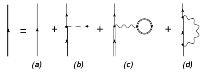
Figure 3: Feynman diagram representation of the Dyson equation of the two point Green function in the many body system corresponding to the Hartree-Fock approximation. The one particle propagator is the sum for the free propagator plus an infinite series of the contributions from a random auxiliary potential (b) and the irreducible self energy of the system in terms of the direct coulomb (c) and exchange (d) contribution. The double lines refer to the mean field propagator while the single ones to the free one.

The self-energy in the mean field approximation is given by the diagrams (b) and (c) in Fig. (3), where the 4 point vertex function contribution is neglected. The mean-field self-energy reads

$$\bar{\Sigma}_{n,n^{\prime}}=-i\int{d\epsilon^{\prime}\over 2\pi}\sum_{m^{\prime},m}\langle n\,m|V|n^{\prime}\,m^{\prime}\rangle\bar{G}(m^{\prime},m;\epsilon^{\prime})\,,$$ (49)

which is energy independent. The tilde here denotes the mean-field approximation of the self-energy and Green’s function. This leads to the field equations of motion from Eq. (48)

$$\left(H_{D}(\bm{r})+V_{nucl}(r)\right)\psi_{n}(\bm{r})+\sum_{m^{\prime}\leq F}\int d\bm{r}^{\prime}\,\psi^{\dagger}_{m^{\prime}}(\bm{r}^{\prime})V_{ee}(|\bm{r}-\bm{r^{\prime}}|)\psi_{[n}(\bm{r^{\prime}})\psi_{m^{\prime}]}(\bm{r})=\varepsilon_{n}\psi_{n}(\bm{r})\,.$$ (50)

III.4 The final state and the core-hole

The final state in the calculation of the transition matrix element plays an important factor on the spectral shapes. There are different ways to treat this problem. A simple approach is to solve for the continuum wave function of the ionized electron in the potential which is calculated from the charge density of the neutral atom, [3]. Typically the neutral atom potential does not have discrete excited states and the simple one electron picture does account for multi-electron correlation effects near the ionization threshold. This results in disagreement with the measured shapes of the ionization cross section close to the ionization threshold, [21], [64].

The excited states of many body systems are studied through the particle-hole or polarization propagator, describing the dynamics of a particle hole moving in a multi particle medium. Typically the random phase approximation with exchange (RPA) reproduces the expected pole structure of the polarization propagator and it has be proven useful in the study of outer atomic shell excitations [12], [18], [56]. RPA with exchange is a good approximation as soon as the electron density of the medium under study is high, [12].

In case of inner shell ionization, where the atomic levels are localized and quite deep in energy, additional collective effects such as the static rearrangement of the bound electrons upon ionization impact the final state heavily. There is extensive literature on theoretical work and experimental validation that relaxation of the atomic orbitals is important during the inelastic scattering in many body systems and in particular in atoms [21, 35, 39, 40, 65, 66, 67]. The core-hole effect has been considered in the analysis of EELS near edge structure spectra, [21, 22, 24, 25, 68] and in X-ray inner shell ionization [69, 70].

A intuitive physical argument motivates such a picture. An ionized electron leaving the atom moves in the field of the created ion where the other bound electrons will rearrange due to the presence of the core-hole. This is an important effect if the ionized electron does not leave the atom well before the bound electrons have the time to relax due to the created vacancy $l$. An order of magnitude estimation shows that for ionized electrons with small kinetic energy, i.e. close to the ionization threshold, this effect plays a role. The relaxation time can be estimated by the energy difference of the neutral atom ground state energy $E_{atom}$, the relaxed ion energy $E_{ion}$ and the vacancy Hartree-Fock eigenenergy $E_{l}$

$$\Delta\tau_{i}\sim{1\over E_{atom}-E_{ion}-E_{l}}$$ (51)

while the characteristic time that a slowly moving ionized electron spends close to the atomic cloud is

$$t_{\epsilon}\sim a_{B}\sqrt{m_{e}\over 2\epsilon}\,.$$ (52)

For $t_{\epsilon}\gtrsim\Delta\tau_{i}$ or equivalently for ionized electron energies smaller than the relaxation of the atom due to the vacancy is important. For fast moving ionized electrons this effect is smaller and the solution approximates the frozen core solution. This is natural since the electromagnetic field of the relaxed and frozen ion has the same asymptotics at large distances.

The effect of the core-hole in the final state can be calculated by perturbation theory of the core-hole potential on the original wave functions of the neutral atom, Appendix (D). The ionized atomic electron state can then be calculated in the field of the ionized atom. An equivalent way is to solve for the ion state with a core-hole self-consistently. Then, solve the equation of motion of the ionized electron in the mean field of the relaxed ion.

$${\widetilde{H}}_{DHF}\,\widetilde{\psi}_{n}(\mathbf{r})-\int d\bm{r}^{\prime}\,{\widetilde{\psi}}^{\dagger}_{l}(\bm{r}^{\prime})V_{ee}(|\mathbf{r}-\mathbf{r}^{\prime}|){\widetilde{\psi}}_{[l}(\mathbf{r}^{\prime})\,{\widetilde{\psi}}_{n]}(\mathbf{r})=\epsilon_{n}\widetilde{\psi}_{n}(\mathbf{r})$$ (53)

where the vacancy is created at the orbital $|l\rangle$ and $\widetilde{H}_{DHF}$ denotes the mean field Hamiltonian in terms of the relaxed orbitals.

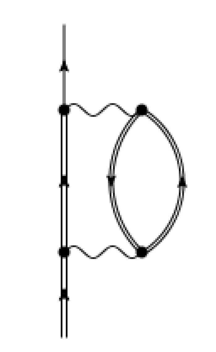
Figure 4: The polarization diagram of the vacancy shell.

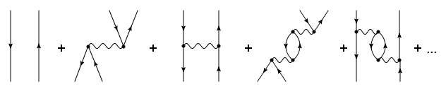
Figure 5: The interaction of the ionized electron and hole pair with the atomic medium is included in the relaxation correction. The opposite arrows refer to the propagation of a particle and hole. The hole is fixed in an inner shell.

The bound and continuum wavefunctions, which are calculated in the presence of the core-hole potential, need to be projected to the orthogonal subspace of the neutral atom eigenstates, Appendix (D). The many body effects due to the core-hole potential are embodied in Eq. (80). The interaction of the core-hole with the atomic orbitals is the main correlation effect beyond the mean field and corresponds to diagrams of the type shown in Fig. (5). Those include the propagation and interaction of the electron-hole pair in the polarized medium. The quantum numbers of the hole orbital are not modified, since it is in a deep shell with a large energy separation from other shells. The vacancy shell is modified by the second-order contribution of the self-energy, as seen in the diagram of Fig. (5). The double lines correspond to the full propagator in the many-particle medium. Those are the two main correlation effects in inner shell ionization. The creation of the core-hole leads to additional dynamical processes such as the decay of the vacancy, emission of secondary electrons and secondary scattering of the ionized electron, [39].

IV Numerical Results

IV.1 Numerical methods

The Dirac-Hartree-Fock system of coupled differential equations is solved numerically in Ambit, an ab-initio, high accuracy atomic structure software library, [57]. There are several other libraries for atomic structure calculations, following different approaches, see [49, 50, 57, 71]. The system of ODEs is solved numerically by the shooting method. A combination of an exponential and linear grid is applied to the radial direction for the solution of the ODEs. The algorithm starts with the normalizable solutions of the wavefunction at practically $r=0$ and $r=\infty$, solves the ODEs outwards and inwards in the integration interval using the Adams-Moulton integration method. The two solutions and their derivatives are matched at the classical turning point of potential, where total energy is equal to the potential. Such normalizable solutions are found for a discrete spectrum of energy eigenvalues. The integration step is repeated, since the Coulomb and exchange interactions are two body interactions which involve the wavefuntions of all the orbitals. When self-consistency is achieved the iteration loop stops. The ionized electron wavefunction is numerically determined in a similar fashion but it does not back-react to the bound state orbitals. The equation of motion is solved numerically with a boundary condition at practical $r=\infty$ which matches a free outgoing spherical wave, for more details see [44], [57].

The occupation of open shells is taken as an average over the quantum numbers of the open shell, such that the spherical symmetry is kept. This approximation is not expected to have a major impact on the overall shape of the ionization cross section of core shells since they are expected to decouple from the valence shells, [19]. The vector coupling of the angular momentum is needed though for the excitation part of the spectra, which are calculated in section (IV.3). The atomic state is written as a Slater determinant, Eq. (20). The auxiliary central field, $U_{ax}$, is chosen to be the Thomas-Fermi potential. The final result does not depend on this choice, but the convergence speed of the numerical integration of the ODEs can substantially improve by a good choice of $U_{ax}$.

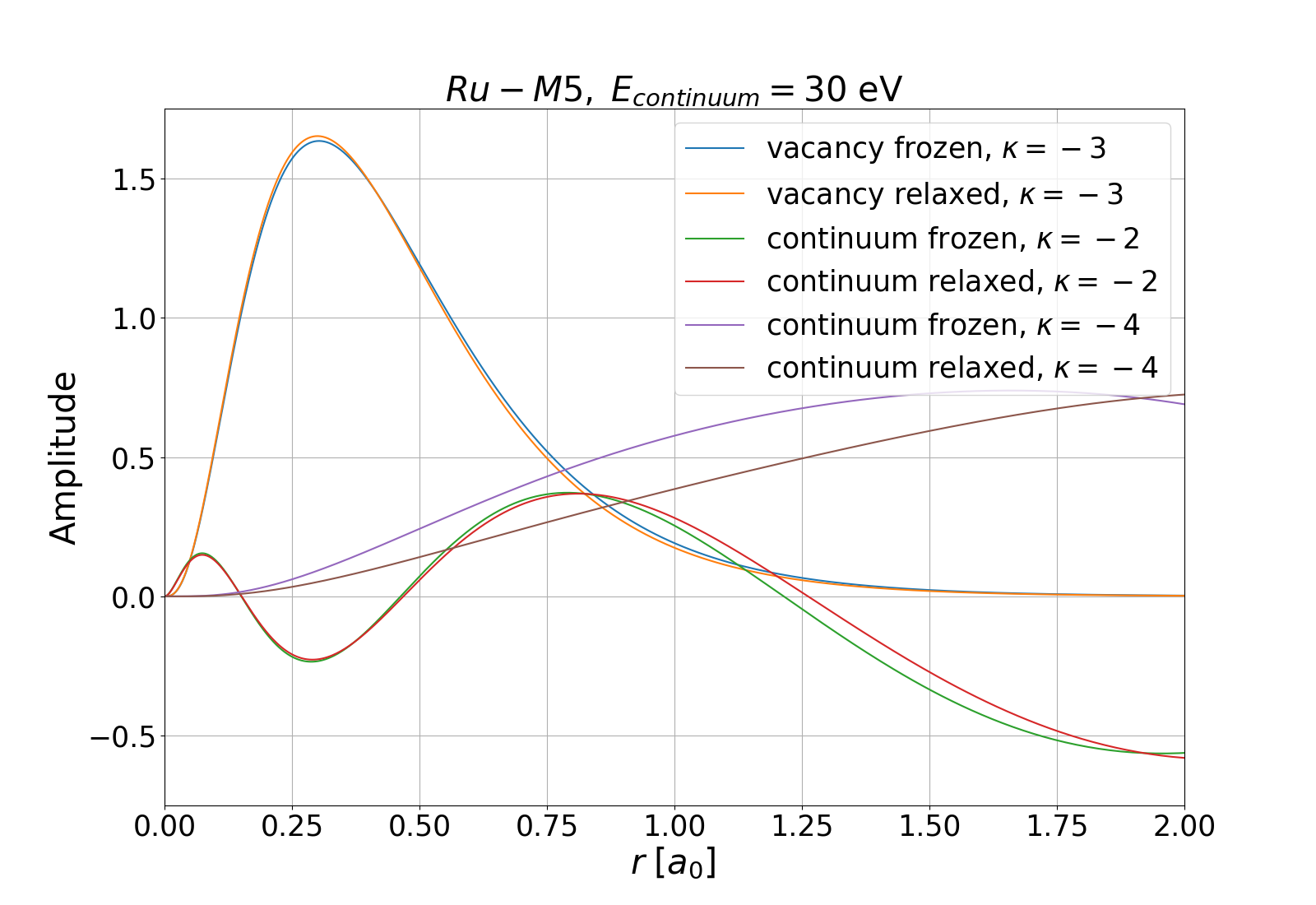
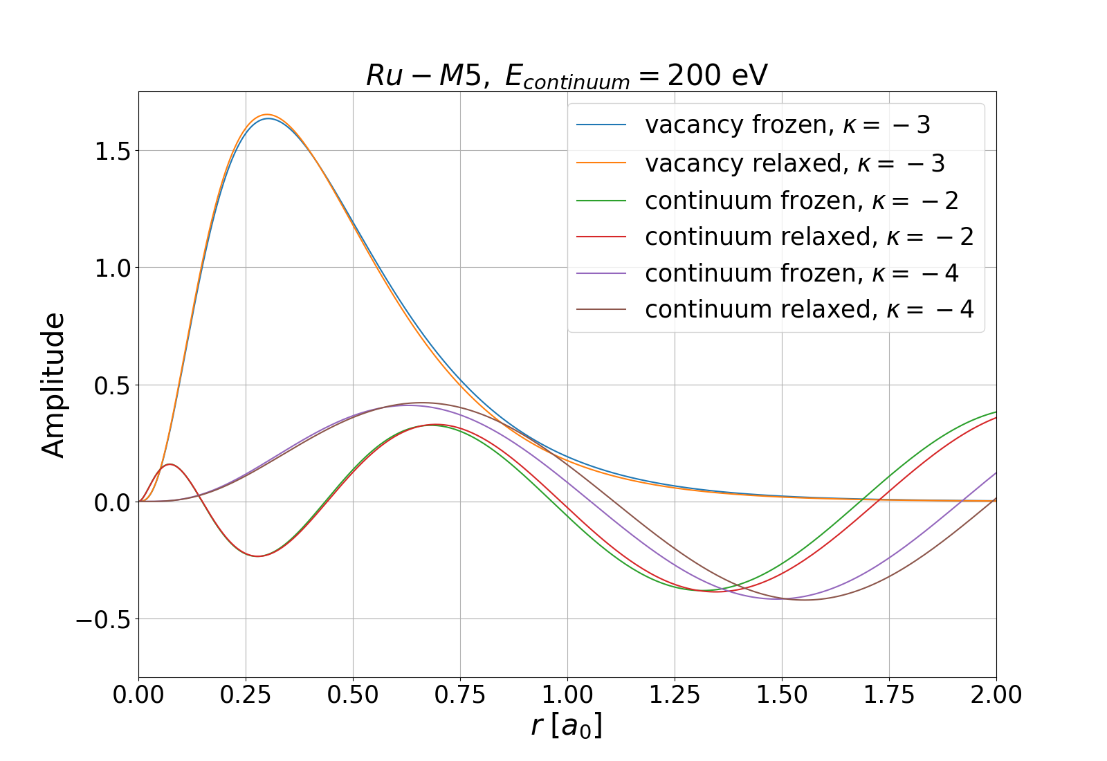
Figure 6: The large component of the Dirac wavefunctions of the Ru-$3d_{5/2}$ orbital and the ionized electron at 30 and 200eV above the ionization threshold for the relaxed and frozen approximation. It is observed that the relaxation due to core-hole affects the ionized electron wavefunction signifficantly.

The rearrangement of the atomic orbitals is explicitly considered by solving Eq.  (53) for the final state. The orthogonality properties of the final state solutions is addressed as typically done in perturbation theory by projecting the perturbed state, due to the core-hole interaction, to the initial state subspace, as described in Appendix (D). In Fig. (6), we show the large component of the Dirac wavefunction of the $3d_{5/2}$, ($\kappa=\pm 3$) Ru subshell in the frozen versus relaxed solution. Moreover, the continuum wavefunction of the ionized electron with $\kappa=\pm 2,\pm 4$ is displayed. This is the continuum state which can be reached by the dipole transition from $3d_{5\over 2}$. We observe that the relaxed and frozen core solutions lead to different continuum wavefunctions in the overlap region with the bound state. This results in a substantial difference in the cross sections for energy loss close to the ionization threshold.

IV.2 Ionization differential cross section

We present here some representative numerical results of the ionization cross section of atoms by fast electrons which are applied to the analysis of EELS data. In Fig. (8), the influence of the dynamical effects of the atomic relaxation and the decay of the core-hole on the ionization cross section is shown. The many-body effects result in a smoother spectral shape close to the ionization threshold. The high energy asymptotics are the same in all the cases, since a high energy outgoing spherical wave is subject to approximately the same potential from the atomic charge density. A microscopic calculation of the initial and final atomic states is performed for the results of this section.

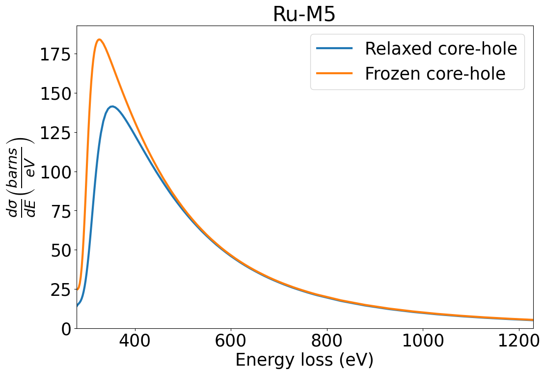
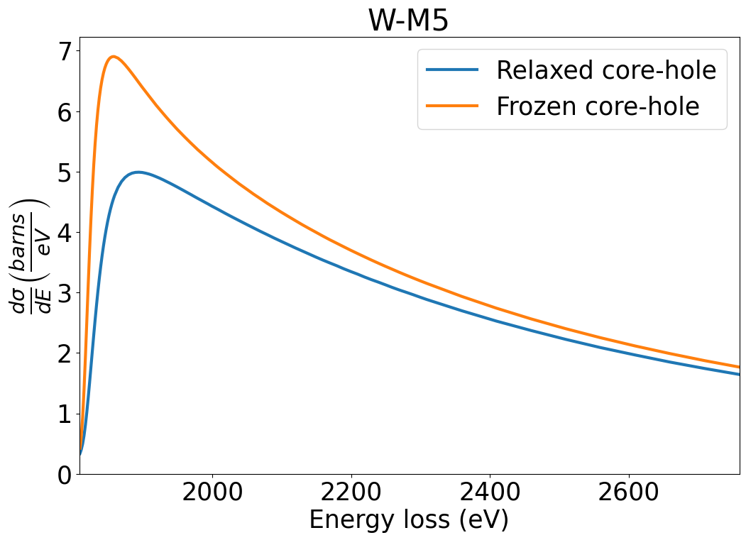
Figure 7: Ru-M5 and W-M5 differential cross section in terms of the ionization energy. Correlation effects such as the polarization and RPA corrections make the spectrum shape smoother close to the ionization threshold. The beam voltage is $300$ keV and the collection angle $100$ mrad.

We present here the differential ionization cross sections for various elements with different configurations of the final state, Figs. (8), (7). In each of those cases, the ionized electron wavefunction is calculated by considering the direct Coulomb and exchange interaction with the atomic bound state. The final bound state electron configurations lead to differences in the spectral shapes of different elements. In the relaxed core-hole case, the core vacancy results in the rearrangement of the atomic orbitals, which are determined by a self-consistent calculation. This is the major dynamic effect in the ionization of inner shells in the typical energy ranges of EELS experiments and influences the spectral shape near the ionization threshold, . In the decayed core-hole case, we have performed an approximate calculation where the core-hole has being filled by vacancy electron. The state of the system is determined by solving the self consistent equations of motion for a relaxed atom of $N-1$ electrons with a vacancy in the valence shell. The ionized electron state is found by considering the explicit interaction with the $N-1$ electrons. A fully consistent calculation would include the explicit calculation of the Auger and the X-ray emission channels which result in either an outgoing Auger electron or a photon in the final state, [39]. This approximation is applicable for deep shells of heavy atoms where the core-hole lifetime is very short compared to the rearrangement time, (51). Those screening effects at the atomic level drive the shape of the cross section close to the ionization threshold.

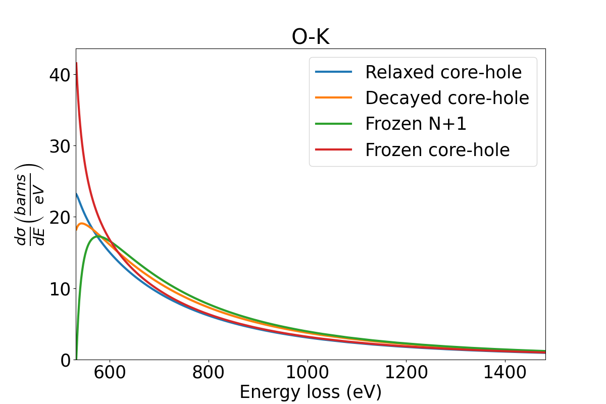
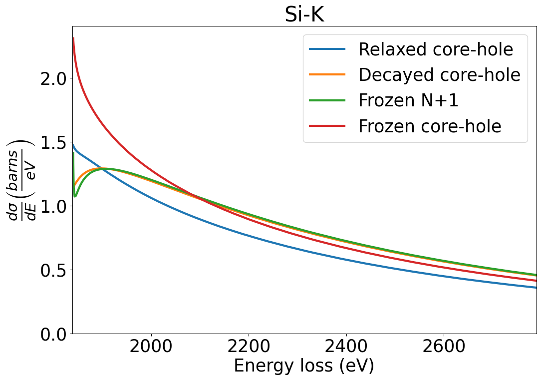
Figure 8: A comparison of the differential ionization cross section in the relaxed case where the atomic orbitals relax under the influence of the core-hole. Relaxed core-hole: the atomic orbitals relax under the influence of the core-hole potential. Decayed core-hole the core-hole has decayed and filled in by a valence electron. Frozen N+1: the final atomic bound states being the same as the neutral atom. Frozen core-hole the final state has one vacancy in the ionized shell but all the orbitals are frozen to their neutral atom form. The beam acceleration voltage is $V_{beam}=300kV$ and the maximum scattering angle is $\theta=100mrad$

In the variations of the frozen approximation the core-hole does not affect the rest of atomic orbitals. In the ”Frozen N+1” case, the final state configuration is made of the neutral atomic core fully filled and the ionized electron. The ”Frozen core-hole” state corresponds to the a configuration with the core-hole present but the atomic orbitals are the same as in the neutral atom. This approximation asymptotes to relaxed result at high energy loss where the electron leaves the atom with high speed, but it deviates close to the ionization threshold, since it does not take into account the dynamics of the core-hole.

The relaxation of the atomic core due to the core-hole can be well described by the $Z+1$ approximation too, [24]. In this case the final atomic state is calculated self-consistently with $Z+1$ nuclear charge.

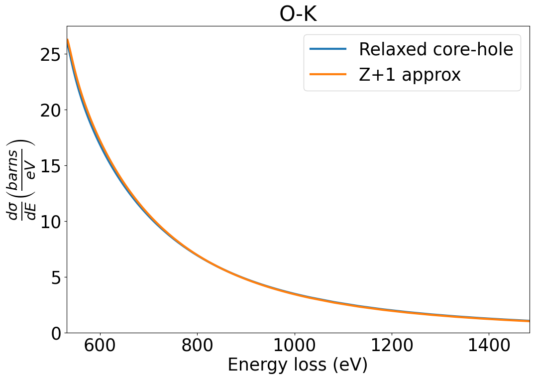
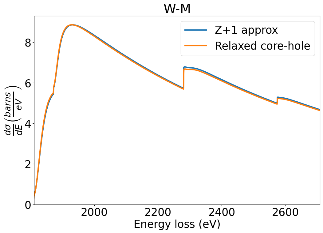
Figure 9: The O-K and W-M ionization differential cross section in the self-consistent explicit relaxed core-hole and Z+1 approximation. The two methods give very similar results. The beam voltage is $300$ kV and the collection angle $100$ mrad.

The differential cross section is also calculated for different acceleration voltages of the incoming electrons. The relativistic kinematics of the beam electrons affect the dependence of the cross section on the beam energy.

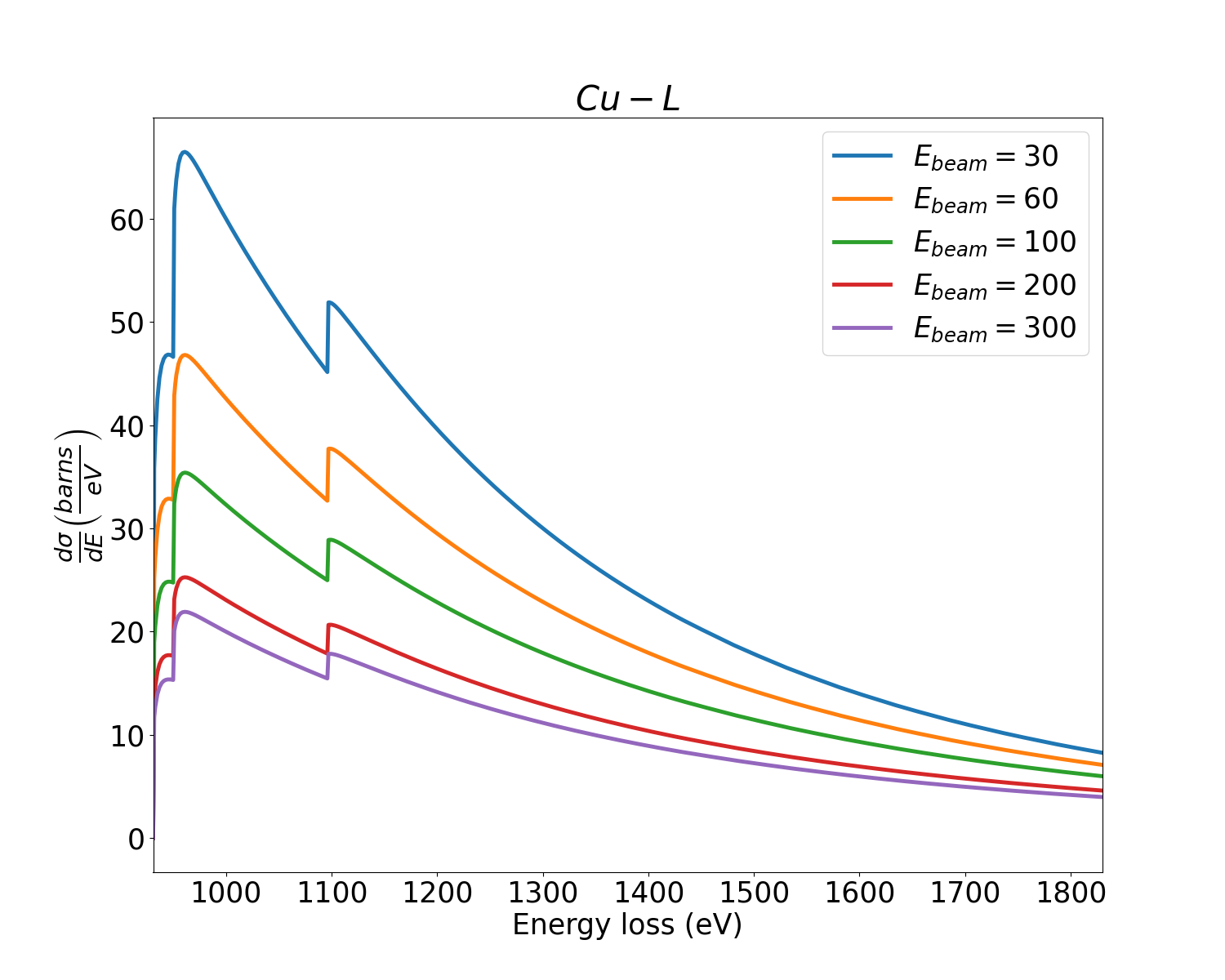
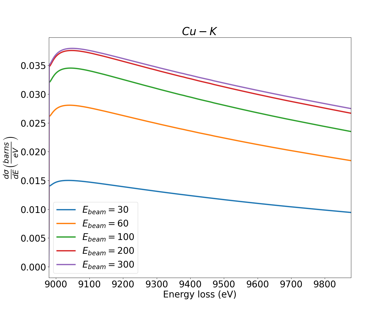
Figure 10: The Cu-L and K differential ionization cross section in terms of the energy loss of the incoming electron. The cross section is calculated for different acceleration energy of the electron beam by including the relaxation of the core-hole. The collection angle is $100$ mrad.

However, the relativistic nature of the problem does not only lie upon the kinematics of the beam. Interesting EELS experiments can be performed at high energy losses or large collection angle. In this case, the momentum transfer $|\mathbf{q}|$ is beyond the dipole approximation and effects from transverse photons are manifest. Fig. (11) shows the contribution of the Coulomb and Transverse electric and magnetic transition matrix elements to the double differential cross section as a function of the effective collection angle $\tilde{\theta}$, Eq. (15). The contribution of the QED part of the matrix element is of the order of $\sim 10\%$. The shape of the double differential cross section is similar to previous results in the literature, [5], but the actual values differ in the case of large energy loss experiments as it seen in the expansion (34). Such corrections are small for the majority of low energy loss EELS experiment.

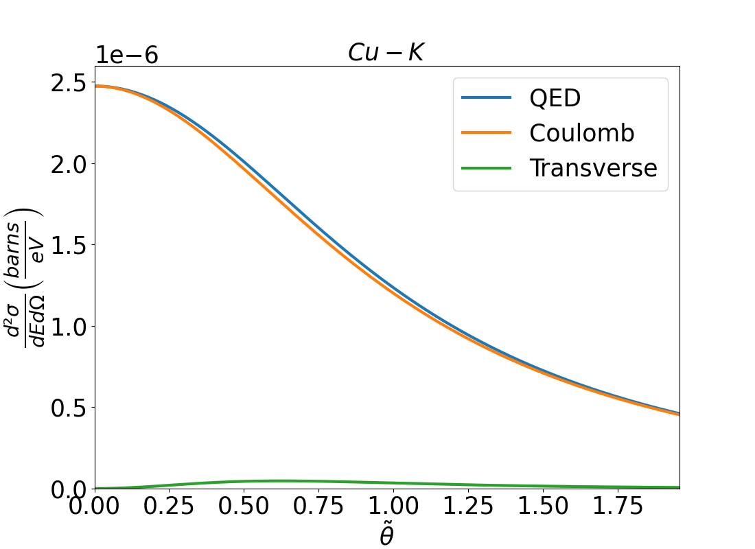
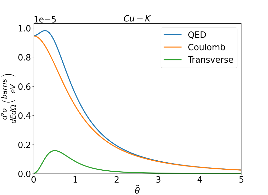
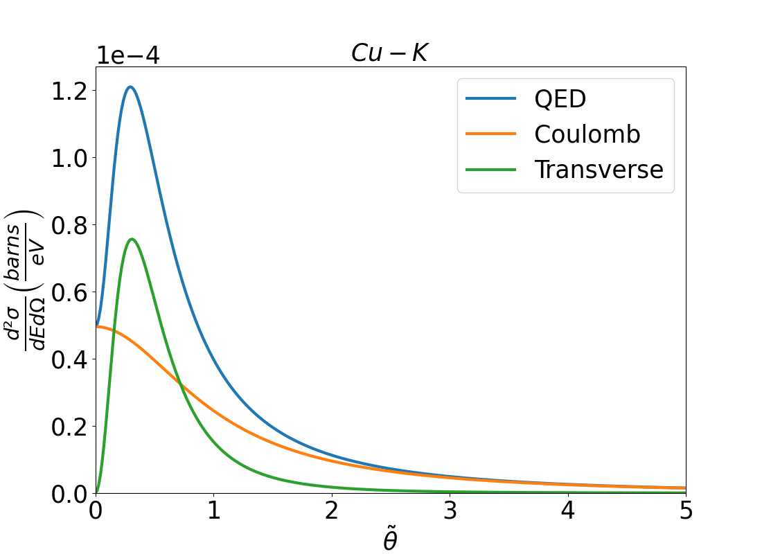
Figure 11: The Cu-K double differential ionization cross section in terms of the effective collection angle, Eq.  (15). The beam voltage is $100,300,1000kV$ and the energy loss is fixed to the ionization threshold of each shell. The shape agrees with previous calculations but the values of the function are different at larger energy losses because the higher order corrections in $C_{L}$ and $C_{T}$ become significant.

Transverse photon corrections are mainly important on the beam-target interaction, but they also contribute to the dynamics of the deep shells of heavy atoms. Those are typically described by effective potentials which are derived from QED. Fig. (12) shows the QED differential cross section in terms of the energy loss. The atomic structure of W is calculated by including the Breit, Uehling potential and electron self energy terms, [57, 59, 60]. Such corrections are small but they can be important in the analysis of the extended fine structure of high energy edges in EELS or XAS, [69, 54].

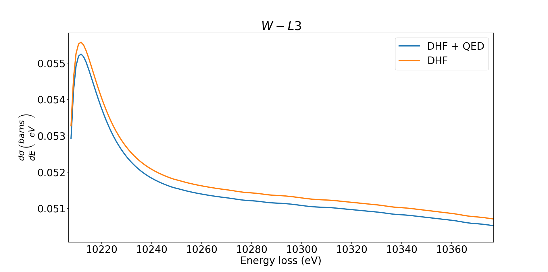
Figure 12: The W-L3 differential ionization cross section in terms of the energy loss. The W atomic structure calculation includes potentials derived from the transverse photon interaction of the bound electrons. The beam voltage is $300kV$.

IV.3 Excitation differential cross section

The near edge structure of EELS and XAS spectra of transition metal and rare earth elements shows a rich excitonic behavior due to the strong interaction of the core-hole and the valence shell electrons, [26, 43]. In this section, we calculate the excitation and ionization differential cross sections of Sc and Dy and compare the result to experimental EELS data. The excitation processes are calculated using the atomic multiplet and crystal field effects in Quanty and Crispy software, [72, 73]. The excitation spectrum of the atom can still be described by local atomic physics because the core-hole in $2p$ or $3d$ interacts strongly with the localized $3d$ or $4f$ electrons, respectively. The initial and final electron configurations of such systems include open shells. Those systems are appropriately described by ${}^{2S+1}L_{J}$ coupled states, which diagonalize the Coulomb and spin-orbit interaction Hamiltonian. The interaction with the ligand atoms is modeled using crystal field theory and the states of the system further split according to their representation under the relevant symmetry. The symmetry group of the $\textrm{ScO}_{3}$ lattice is $O_{h}$. The ionization part of the differential cross section is calculated as before by including the relaxation effects due to the core-hole.

The inelastic cross section, that includes transitions to the open valence 3d/4f shells and to the continuum, is plotted versus an EELS spectrum of $\textrm{DyScO}_{3}$, Fig. (13). We here focus on the theoretical calculation of the excitation and ionization differntial cross section and the comparison to an experimental spectrum. For a detailed presentation of EELS data analysis methodology see [74, 75, 76]. We here remove the continuous background and fit the broadened theoretical differential cross sections to the Sc, O and Dy experimental data. The experiment was carried out with an Iliad Energy Filter at beam voltage $300kV$ and relatively low resolution. The energy per spectrum channel is 1 eV. The atomic multiplet and crystal field calculation depends on the crystal field splitting. By fitting the cross section to the data we find the overall intensity of the cross section which depends on the number of atoms in the material and the cystal field parameter. The 3d splitting of Sc is found to be 1.7eV, in close agreement with the result from the fitting to high resolution XAS data, [42]. Such results indicate that elementary knowledge of the electronic structure of materials, such as the crystal field splitting, can be derived from lower energy resolution experiments when appropriately calculated theoretical models are applied. Measuring the intensity of the near edge region of transition metal and lanthanide elements will also enhance the EELS analysis aiming at the elemental composition of a sample, [77].

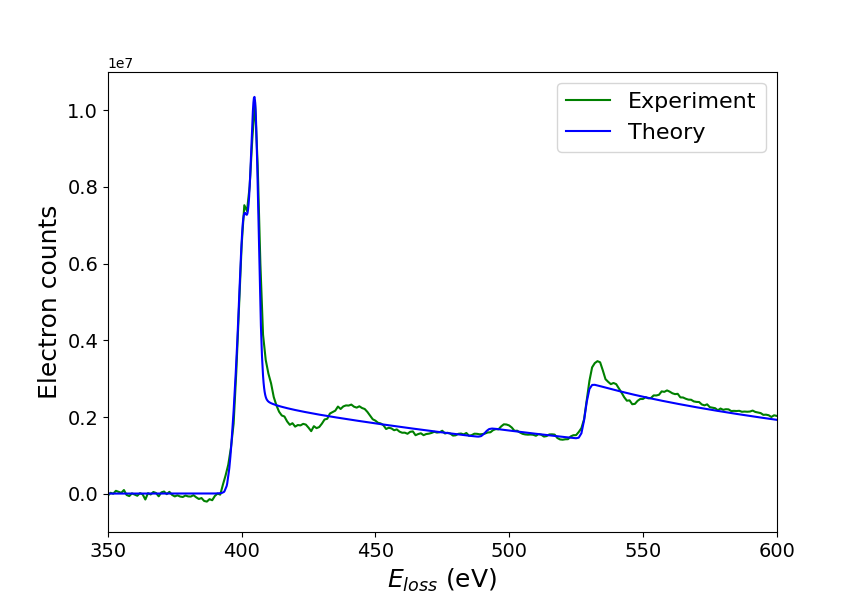
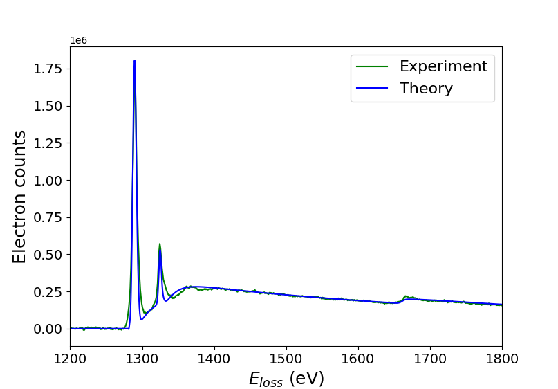
Figure 13: The Sc-2p, O-1s and Dy-3d inelastic cross section by an electron beam vs experimental EELS data. The theoretical calculation of Sc-2p and Dy-3d includes the transition to the narrow 3d/4f valence band ($2p^{6}3d^{0}\to 2p^{5}3d^{1}$ and $3d^{10}4f^{0}\to 3d^{9}4f^{1}$ respectively) and the continuum. The peak intensities and the continuum part of the cross section are in close agreement with the data. The crystal field splitting of Sc$3+$ is found to be $1.7eV$. The O-1s near edge fine structure is not included in this calculation.

A detailed calculation of the transition matrix elements should in principle include the coupling of the discrete and continuum final states, [78]. Here, we consider a simplified case, where the excitation peaks of the spectrum do not interact with the continuum. The coupling of discrete and continuous states is the reason for the asymmetry which is observed in the tails of the peaks in the experimental data. Such effects will be addressed in future work. Part of the asymmetry in the experimental data is also due to multiple scattering which is typically addressed by convolving the theoretical models with the low loss EELS spectrum and then fit to the data.

V Summary and Discussion

In this work, we present a detailed study of the inelastic scattering of a relativistic electron beam from a generic target. The results can be applied to the analysis of core loss EELS spectra. The most general form of the inelastic cross section is calculated in Quantum Electrodynamics in terms of the irreducible tensor operators of the target electromagnetic transition current. The tree level Feynman diagram is adequate for EELS experiments since the momentum transfer is always $|\mathbf{q}|\ll m$, where $m\sim 511$ keV is the electron mass. However, we have not made any other assumptions about the magnitude of $|\mathbf{q}|$ in our general result, Eqs (14, 26) . Existing relativistic calculations have focused on the dipole approximation, $|\mathbf{q}|a_{B}\ll 1$, or the case when only the transition current component along the incoming beam direction is considered, $|\mathbf{q}|\ll|\mathbf{p}|$. We have also expanded here the general cross section as a series of the effective scattering angle $\tilde{\theta}$ and energy loss $E$. Higher-order corrections become more important for EELS data at higher energy losses and large collection angles. Our calculation applies to a wide range of experimental conditions, including beam energies up to the MeV scale.

The calculation of the atomic structure is performed from a microscopic perspective within the relaxed Dirac-Hartree-Fock approach, [57]. The Dirac equation has been solved for all atoms, considering coulomb and exchange interactions among electrons, as well as electron-nucleus interactions. Additionally, QED corrections to the electron-electron potential, such as the Breit term, are shown to have a non-zero but small impact on the orbital wave functions of relatively deep shells in heavy atoms, which can be probed in EELS.

An important part of our calculation is the microscopic calculation of many-body effects for the ionization of core shell of all atoms in the periodic table. The random phase approximation with exchange is known to describe well the valence shell ionization of atoms, [18]. The shape of the inner shell ionization spectra is mostly influenced by the static rearrangement of the atomic orbitals due to the core-hole, [41]. The interaction of the ionized electron with the atom, is screened by the relaxation of the bound state electrons. This results in a lower cross section close to the ionization threshold, which is agreement with the expectation from experiments. It has been noticed that in ionization experiments the one electron theoretical models overestimate the edges close to the ionization energy, especially for intermediate shells. This may lead to less accurate disentanglement of overlapping or close edges in the EEL spectra. An equivalent method to include such correlation effects in those calculations is by using the $Z+1$ approximation, where the final state is approximated by the bound orbitals of a $Z+1$ atom and an outgoing, ionized electron, [24].

The core-hole opens up decay channels in this process such as the X-ray emission and Auger decays of the final state. In principle, those effects can become important close to the ionization threshold, if their lifetime is comparable to the rearrangement time of the core-hole, [41]. Future work will address the core-hole decay in detail by generalizing the current calculation.

Beyond the elemental composition of a material, higher energy resolution EELS experiments reveal information about its electronic structure. An important class of such experiments involves transition metal and rare earth oxides. It is typical for these elements to exhibit excitonic effects in their $2p$ and $3d$ spectra due to the significant overlap of the valence shells with the ionized core shell. These effects can be described by the atomic multiplet crystal field theory, [26]. In this context, the vector coupling of multiple valence electron orbitals and their overlap with the initial state account for the major part of the excitonic peaks in the spectrum. The interaction with the ligands can be addressed in the context of crystal field theory. Additional contributions due to charge transfer from the ligands are important in certain compounds. We have calculated the excitation and ionization spectra of Sc $2p$ and Dy $3d$ edges and compared to relatively low resolution resolution EELS data. In this case all the fine structure peaks are not resolved but fitting the crystal field parameter to the data of Sc edge agrees closely with the previous results from higher resolution XAS analysis, [42].

Appendix A The Feynman diagram

The Dyson equation for the S-matrix of electron scattering with a composite system is defined in terms of the asymptotically stationary states, [79], [80]

$$S_{\beta\alpha}=\langle\psi^{-}_{\beta}|\psi^{+}_{\alpha}\rangle\,.$$ (54)

The S-matrix operator is then

$$S=1+\sum_{n=1}^{\infty}\frac{(-i)^{n}}{n!}\int_{-\infty}^{\infty}dt_{1}\ldots dt_{n}T\{H_{int}(t_{1})\ldots H_{int}(t_{n})\}\,,$$ (55)

where $H_{int}(t)$ is the interaction Hamiltonian, which is derived from the Lagrangian in Eq. (1)

$$H_{int}(t)=\int d^{3}x\,\mathcal{J}^{\mu}(t,{\bf x})A_{\mu}(t,{\bf x})+ie\,\int d^{3}x\,\bar{\Psi}(t,{\bf x})\not{A}(t,{\bf x})\Psi(t,{\bf x})$$ (56)

Dyson equation, (55), for $n=1$, is applied to calculate the S-matrix between the initial and final states, $|p_{i}m_{s_{i}}\rangle\otimes|\alpha\rangle$ and $|p_{f}m_{s_{f}}\rangle\otimes|\beta\rangle$. This directly leads to

$$S_{p_{f},m_{s_{f}},\,\beta\,;\,p_{i},m_{s_{i}},\,\alpha}= {(-i)^{2}\over 2!}2\int d^{4}x_{1}d^{4}x_{2}e^{-ip_{f}x_{1}}\bar{u}(p_{f},m_{s_{f}})ie\,\gamma^{\mu}e^{ip_{i}x_{1}}u(p_{i},m_{s_{i}})(-i)\Delta_{\mu\nu}(x_{1},x_{2})\langle\beta|\mathcal{J}_{\mu}(x_{2})|\alpha\rangle\$$ (57)

where $\psi_{p,m_{s}}(x)=e^{ipx}u(p,m_{s})$ is the plane wave solution of the free Dirac equation, and the photon propagator in coordinate space reads is

$$\Delta_{\mu\nu}(x_{1},x_{2})=\int{d^{4}q\over(2\pi)^{4}}{\eta_{\mu\nu}\over q^{2}-i\varepsilon}e^{iq(x_{1}-x_{2})}\,.$$ (58)

The photon-fermion vertex is $(2\pi)^{4}e\gamma^{\mu}\delta\left(\sum p\right)$ while the coupling with the external current results in vertex $(2\pi)^{4}\langle\beta|\mathcal{J}_{\mu}(x)|\alpha\rangle\$. The S-matrix then reads

$$S_{p_{f},s_{f},\,\beta\,;\,p_{i},s_{i},\,\alpha} =-{e\over(2\pi)^{3}}{\bar{u}(p_{f},m_{s_{f}})\gamma_{\mu}u(p_{i},m_{s_{i}})\over q^{2}-i\varepsilon}\int d^{4}xe^{-iqx}\langle\beta|\mathcal{J}_{\mu}(x)|\alpha\rangle\ \,.$$ (59)

From the definition (3) the transition matrix is

$$|T_{p_{f},\,\beta\,;\,p_{i},\,\alpha}|^{2} ={1\over 2}\sum_{m_{s_{i}},m_{s_{f}}}|T_{p_{f},m_{s_{f}},\,\beta\,;\,p_{i},m_{s_{i}},\,\alpha}|^{2}$$

$$={e^{2}\over 2}\sum_{m_{s_{i}},m_{s_{f}}}{\bar{u}(p_{f},m_{s_{f}})\gamma^{\mu}u(p_{i},m_{s_{i}})\bar{u}(p_{i},m_{s_{i}})\beta\gamma^{\nu}\beta u(p_{f},m_{s_{f}})\over q^{4}}\langle\beta|\mathcal{J}_{\mu}(\mathbf{q})|\alpha\rangle\,\langle\beta|\mathcal{J}_{\nu}^{\dagger}(\mathbf{q})|\alpha\rangle$$

$$=-{e^{2}\over 2q^{4}}{\mathrm{T}r}\left(\gamma^{\mu}{-i{\not{p}_{i}}+m\over 2E_{i}}\gamma^{\nu}{-i{\not{p}_{f}}+m\over 2E_{f}}\right)\langle\beta|\mathcal{J}_{\mu}(\mathbf{q})|\alpha\rangle\,\langle\beta|\mathcal{J}_{\nu}^{\dagger}(\mathbf{q})|\alpha\rangle$$ (60)

The trace of the products of gamma matrices is readily derived from their commutation relations

$${\mathrm{T}r}\left(\gamma^{\mu}\gamma^{\nu}\right)=\eta^{\mu\nu}\,\,,\,\,\,{\mathrm{T}r}\left(\gamma^{\mu}\gamma^{\nu}\gamma^{\rho}\gamma^{\sigma}\right)=4\left(\eta^{\mu\nu}\eta^{\rho\sigma}-\eta^{\mu\rho}\eta^{\nu\sigma}+\eta^{\mu\sigma}\eta^{\nu\rho}\right)$$ (61)

The T-matrix in terms of the electromagnetic 4-current then becomes

$$|T_{p_{f},\,\beta\,;\,p_{i},\,\alpha}|^{2}=-{e^{2}\over 2q^{4}}{1\over E_{i}E_{f}}\left((p_{i}\cdot p_{f}+m^{2})|\mathcal{J}_{\beta\alpha}|^{2}-p_{i}\cdot\mathcal{J}_{\beta\alpha}\,p_{f}\cdot\mathcal{J}_{\beta\alpha}^{\dagger}-p_{i}\cdot\mathcal{J}_{\beta\alpha}^{\dagger}\,\,p_{f}\cdot\mathcal{J}_{\beta\alpha}\right)\,.$$ (62)

Appendix B The multipole expansion derivation for Dirac orbitals

Eq. (26) is a general expression of the relavant transition matrix elements in terms of the irreducible operators of the rotation group. We here calculate such matrix elements for Dirac wavefunctions. Similar derivation have been followed for photoionization and photon emission of atoms with slightly different methods, [11], [51]. Inserting the expression of the 4-current, Eqs. (24), (25) in the T-matrix elements (13)

$$\langle m||T_{J}^{(mag)}||n\rangle= i\,e\,\left[\langle\kappa_{m}||\left[\mathbf{Y}_{J\,J}\cdot\bm{\sigma}\right]||-\kappa_{n}\rangle\int dr\,r^{2}\,j_{J}\left(|\mathbf{q}|r\right)F_{m}^{\dagger}(r)G_{n}(r)\right.$$

$$\left.-\langle-\kappa_{m}||\left[\mathbf{Y}_{J\,J}\cdot\bm{\sigma}\right]||\kappa_{n}\rangle\int dr\,r^{2}\,j_{J}\left(|\mathbf{q}|r\right)G_{m}^{\dagger}(r)F_{n}(r)\right]$$ (63)

$$\langle m||T_{J}^{(el)}||n\rangle= i\,e\,\sqrt{J+1\over 2J+1}\left[\langle\kappa_{m}||\left[\mathbf{Y}_{J\,J-1}\cdot\bm{\sigma}\right]||-\kappa_{n}\rangle\int dr\,r^{2}\,j_{J-1}\left(|\mathbf{q}|r\right)F_{m}^{\dagger}(r)G_{n}(r)\right.$$

$$-\left.\langle-\kappa_{m}||\left[\mathbf{Y}_{J\,J-1}\cdot\bm{\sigma}\right]||\kappa_{n}\rangle\int dr\,r^{2}\,j_{J-1}\left(|\mathbf{q}|r\right)G_{m}^{\dagger}(r)F_{n}(r)\right]$$

$$-i\,e\,\sqrt{J\over 2J+1}\left[\langle\kappa_{m}||\left[\mathbf{Y}_{J\,J+1}\cdot\bm{\sigma}\right]||-\kappa_{n}\rangle\int dr\,r^{2}\,j_{J+1}\left(|\mathbf{q}|r\right)F_{m}^{\dagger}(r)G_{n}(r)\right.$$

$$+\left.\langle-\kappa_{m}||\left[\mathbf{Y}_{J\,J+1}\cdot\bm{\sigma}\right]||\kappa_{n}\rangle\int dr\,r^{2}\,j_{J+1}\left(|\mathbf{q}|r\right)G_{m}^{\dagger}(r)F_{n}(r)\right]$$ (64)

In those expressions, we notice the irreducible matrix element of the tensor operator which is the inner product of a vector spherical harmonic and the spin operator. This is decomposed to matrix elements of the operators $Y_{L=J,J\pm 1}$ and $\sigma$, which act on the coordinate and spin space respectively, [81]

$$\langle j^{\prime},\ell^{\prime},\frac{1}{2}||\mathbf{Y_{J\,L}}\cdot\bm{\sigma}||j,\ell,\frac{1}{2}\rangle=[j^{\prime},J,j]\begin{Bmatrix}\ell^{\prime}&\ell&L\\ {1\over 2}&{1\over 2}&1\\ j^{\prime}&j&J\end{Bmatrix}\langle j^{\prime},\ell^{\prime}||Y_{L}||j,\ell\rangle\langle\frac{1}{2}||\sigma||\frac{1}{2}\rangle$$ (65)

Applying Eq. (27) and $\langle{1\over 2}||\sigma||{1\over 2}\rangle=\sqrt{6}$ we find

$$\langle m||T_{J}^{(mag)}||n\rangle =i\,e\,\left[j_{m},\,J,\,j_{n}\right]^{1\over 2}\langle{1\over 2}||\sigma||{1\over 2}\rangle$$

$$\left[\langle\kappa_{m}||Y_{J}||-\kappa_{n}\rangle\begin{Bmatrix}\ell_{m}^{-}&\ell_{n}^{+}&J\\ {1\over 2}&{1\over 2}&1\\ j_{m}&j_{n}&J\end{Bmatrix}\int dr\,r^{2}\,j_{J}\left(|\mathbf{q}|r\right)F_{\beta}^{\dagger}(r)G_{\alpha}(r)\right.$$

$$\left.-\langle-\kappa_{m}||Y_{J}||\kappa_{n}\rangle\begin{Bmatrix}\ell_{m}^{+}&\ell_{n}^{-}&J\\ {1\over 2}&{1\over 2}&1\\ j_{m}&j_{n}&J\end{Bmatrix}\int dr\,r^{2}\,j_{J}\left(|\mathbf{q}|r\right)G_{\beta}^{\dagger}(r)F_{\alpha}(r)\right]$$

$$=i\,e\,(-1)^{\ell^{-}_{m}}\sqrt{\left[j_{m},\,J,\,j_{n}\right]\over 4\pi}\Pi(\ell^{-}_{m},J,\ell^{+}_{n})$$

$$\times\left[\sqrt{6\,[\ell^{-}_{m},\,J,\,\ell^{+}_{n}]}\begin{pmatrix}\ell^{-}_{m}&J&\ell^{+}_{n}\\ 0&0&0\end{pmatrix}\begin{Bmatrix}\ell^{-}_{m}&\ell^{+}_{n}&J\\ {1\over 2}&{1\over 2}&1\\ j_{m}&j_{n}&J\end{Bmatrix}\right.\int dr\,r^{2}\,j_{J}\left(|\mathbf{q}|r\right)F_{m}(r)G_{\nu}(r)$$

$$\left.+\sqrt{6\,[\ell^{+}_{m},\,J,\,\ell^{-}_{n}]}\begin{pmatrix}\ell^{+}_{m}&J&\ell^{-}_{n}\\ 0&0&0\end{pmatrix}\begin{Bmatrix}\ell^{+}_{m}&\ell^{-}_{n}&J\\ {1\over 2}&{1\over 2}&1\\ j_{m}&j_{n}&J\end{Bmatrix}\int dr\,r^{2}\,j_{J}\left(|\mathbf{q}|r\right)G_{m}(r)F_{n}(r)\right]$$

$$= -i\,e\,(-1)^{j_{m}+1/2}\sqrt{\left[j_{m},\,J,\,j_{n}\right]\over 4\pi}\begin{pmatrix}j_{m}&j_{n}&J\\ -{1\over 2}&{1\over 2}&0\end{pmatrix}\Pi(\ell^{-}_{m},J,\ell^{+}_{n}){(\kappa_{n}+\kappa_{m})\over\sqrt{J(J+1)}}$$

$$\times\int dr\,r^{2}\,j_{J}\left(|\mathbf{q}|r\right)\left(F_{m}(r)G_{n}(r)+G_{m}(r)F_{n}(r)\right)$$ (66)

where $[x,y,\ldots]=(2x+1)(2y+1)\ldots$ and $\Pi(\ell^{-}_{m},J,\ell^{+}_{n})=1$ for $\ell^{-}_{m}+J+\ell^{+}_{n}=2n$ and $0$ otherwise. Notice $\ell^{\pm}=J\mp{\mathrm{sgn}(\kappa)\over 2}$ and $J=\mathrm{sgn}(\kappa)\,\kappa-{1\over 2}$. The following identity for the reduction of 9-j to the 3-j Wigner symbols, [81], was used

$$\sqrt{6\,[J,\,\ell_{m},\,\ell_{n}]}\begin{pmatrix}J&\ell_{m}&\ell_{n}\\ 0&0&0\end{pmatrix}\begin{Bmatrix}\ell_{m}&\ell_{n}&J\\ {1\over 2}&{1\over 2}&1\\ j_{m}&j_{n}&J\end{Bmatrix}=\begin{pmatrix}j_{m}&j_{n}&J\\ {1\over 2}&{1\over 2}&-1\end{pmatrix}.$$ (67)

The electric T-matrix reads

$$\langle m||T_{J}^{(el)}||n\rangle =i\,e\,\left[j_{m},\,J,\,j_{n}\right]^{1\over 2}\langle{1\over 2}||\sigma||{1\over 2}\rangle$$

$$\left[\sqrt{J+1\over 2J+1}\,\langle\kappa_{m}||Y_{J-1}||-\kappa_{n}\rangle\begin{Bmatrix}\ell^{-}_{m}&\ell^{+}_{n}&J-1\\ {1\over 2}&{1\over 2}&1\\ j_{m}&j_{n}&J\end{Bmatrix}\right.\int dr\,r^{2}\,j_{J-1}\left(|\mathbf{q}|r\right)F_{m}^{\dagger}(r)G_{n}(r)$$

$$-\sqrt{J+1\over 2J+1}\,\langle-\kappa_{\beta}||Y_{J-1}||\kappa_{\alpha}\rangle\begin{Bmatrix}\ell^{+}_{m}&\ell^{-}_{n}&J-1\\ {1\over 2}&{1\over 2}&1\\ j_{m}&j_{n}&J\end{Bmatrix}\int dr\,r^{2}\,j_{J-1}\left(|\mathbf{q}|r\right)G_{m}^{\dagger}(r)F_{n}(r)$$

$$-\sqrt{J\over 2J+1}\,\,\langle\kappa_{m}||Y_{J+1}||-\kappa_{n}\rangle\begin{Bmatrix}\ell^{-}_{m}&\ell^{+}_{n}&J+1\\ {1\over 2}&{1\over 2}&1\\ j_{m}&j_{n}&J\end{Bmatrix}\int dr\,r^{2}\,j_{J+1}\left(|\mathbf{q}|r\right)F_{m}^{\dagger}(r)G_{n}(r)$$

$$\left.+\sqrt{J\over 2J+1}\,\langle-\kappa_{m}||Y_{J+1}||\kappa_{n}\rangle\begin{Bmatrix}\ell^{+}_{m}&\ell^{-}_{n}&J+1\\ {1\over 2}&{1\over 2}&1\\ j_{m}&j_{n}&J\end{Bmatrix}\int dr\,r^{2}\,j_{J+1}\left(|\mathbf{q}|r\right)G_{m}^{\dagger}(r)F_{n}(r)\right]\,.$$ (68)

The 9-j symbols are reduced using the identity [82]

$$\sqrt{6\,[J\pm 1,\,\ell_{m},\,\ell_{n}]}\begin{pmatrix}J\pm 1&\ell_{m}&\ell_{n}\\ 0&0&0\end{pmatrix}\begin{Bmatrix}\ell_{m}&\ell_{n}&J\\ {1\over 2}&{1\over 2}&1\\ j_{m}&j_{n}&J\pm 1\end{Bmatrix}$$

$$=\frac{(\ell_{m}-j_{m})(2j_{m}+1)+(\ell_{n}-j_{n})(2j_{n}+1)\pm J\pm\frac{1}{2}+\frac{1}{2}}{(2J+1)(J\pm\frac{1}{2}-\frac{1}{2})}\begin{pmatrix}j_{m}&j_{n}&J\\ {1\over 2}&{1\over 2}&-1\end{pmatrix}\,.$$ (69)

The electric matrix element then reduces to

$$\langle m||T_{J}^{(el)}||n\rangle= -i\,e\,(-1)^{j_{m}+1/2}\sqrt{\left[j_{m},\,J,\,j_{n}\right]\over 4\pi}\begin{pmatrix}j_{m}&j_{n}&J\\ -{1\over 2}&{1\over 2}&0\end{pmatrix}\Pi(\ell^{-}_{m},J,\ell^{-}_{n})$$

$$\times\left[{\kappa_{n}-\kappa_{m}\over\sqrt{J(J+1)}}\int dr\,r^{2}\,{(J+1)j_{J-1}\left(|\mathbf{q}|r\right)-Jj_{J+1}\left(|\mathbf{q}|r\right)\over 2J+1}\left(F_{m}(r)G_{n}(r)+G_{m}(r)F_{n}(r)\right)\right.$$

$$\left.+\sqrt{J(J+1)}\int dr\,r^{2}\,{j_{J-1}\left(|\mathbf{q}|r\right)+j_{J+1}\left(|\mathbf{q}|r\right)\over 2J+1}\left(F_{m}(r)G_{n}(r)-G_{m}(r)F_{n}(r)\right)\right]\,.$$ (70)

Appendix C General multi-electron matrix elements

The interaction of the electron beam with the target multi-electron atom is expressed by one-body operators. The matrix element of such operators between the initial and final multi-electron wavefunctions, $|\alpha\rangle$ and $|\beta\rangle$, is calculated here. Since the atomic orbitals rearrange themselves, after the excitation or ionization of the system, the initial and final orbitals are not orthogonal and the relevant transition matrix elements are slightly more complicated, [27]. An explicit derivation for fully antisymmetric wavefunctions, written as Slater determinants, is presented below for the sake of clarity.
For any one body operator

$${\it O}=\sum_{m,\,n}\langle m|{\it O}|n\rangle a^{\dagger}_{m}a_{n}$$ (71)

in two orthonormal bases ${|\alpha\rangle}$ and ${|\beta\rangle}$. We calculate the matrix element $\langle\Psi_{f}|{\it O}|\Psi_{i}\rangle$, where Slater initial and final states are used, 20. The creation operator of a state $\chi$ in an N particle state acts like

$$a^{\dagger}_{\chi}|\psi_{1}\ldots\psi_{N}\rangle=|\chi\psi_{1}\ldots\psi_{N}\rangle$$ (72)

By taking the hermitian conjugate of the equation above and multiply with an arbitrary (N-1) bra state on the left one can show

$$a_{\chi}|\psi_{1}\ldots\psi_{N}\rangle=\sum_{k}(-1)^{k-1}\langle\chi|\psi_{k}\rangle\,|\psi_{1}\ldots\psi_{k-1}\psi_{k+1}\ldots\psi_{N}\rangle$$ (73)

The two equations above imply

$$\langle\widetilde{\Psi}_{\beta}|{\it O}|\Psi_{\alpha}\rangle=\langle\widetilde{\psi}_{1}\ldots\widetilde{\psi}_{N}|{\it O}|\psi_{1}\ldots\psi_{N}\rangle=\sum_{i,j}\langle\widetilde{\psi}_{i}|{\it O}|\psi_{j}\rangle(-1)^{i+j}S_{ij}\,,$$ (74)

where

$$S_{ij}=\sum_{P}(-1)^{P}\prod\limits_{\begin{subarray}{c}k=1\\ k\neq i\,,P(k)\neq j\end{subarray}}^{N}\langle\widetilde{\psi}_{k}|\psi_{P(k)}\rangle$$ (75)

Appendix D The core-hole perturbation

We revisit the perturbative expansion of the core-hole interaction and how this matches the variational approach, which is typically employed for this calculation, [12]. The Dirac-Hartree-Fock equations of motion in the presence of a core-hole potential are given in Eq. (53), where the the contribution of the electron and core-hole interaction has been removed from Eqs. (50). When $n\leq F$ the backreaction of the ionized electron to the bound states is not considered. Using the completeness relation of the unperturbed atomic orbitals, Eq. (53) becomes

$$\widetilde{H}_{DHF}\,\widetilde{\psi}_{n}(\mathbf{r})-\sum_{m>F}\psi_{m}(\mathbf{r})\langle{\widetilde{l}}\,m|V_{ee}|\widetilde{l}\,\widetilde{n}\rangle=\tilde{\epsilon}_{n}\widetilde{\psi}_{n}(\mathbf{r})$$ (76)

where the orthogonality of the full eigenstates to the unperturbed ones is imposed by restricting the sum over $m$ to unoccupied states. The matrix element of the two body interaction between $|n\rangle$ and $|m\rangle$ includes the direct and exchange terms

$$\langle\tilde{l}\,m|V_{ee}|\tilde{l}\,\tilde{n}\rangle =\int d\bm{r}^{\prime\prime}\int d\bm{r}^{\prime}\widetilde{\psi}^{\dagger}_{l}(\bm{r}^{\prime})\psi^{\dagger}_{m}(\bm{r}^{\prime\prime})V_{ee}(|\bm{r}-\bm{r^{\prime}}|)\widetilde{\psi}_{[l}(\mathbf{r}^{\prime})\widetilde{\psi}_{n]}(\mathbf{r}^{\prime\prime})=\widetilde{g}_{lm[ln]}$$ (77)

The equation of motion can be rewritten in terms of the unperturbed wavefunctions

$$H_{DHF}\,\widetilde{\psi}_{n}(\mathbf{r})+\sum_{m>F}\psi_{m}(\mathbf{r})\left(\sum_{j\leq F,\,j\neq l}\langle\widetilde{j}\,m|V_{ee}|\widetilde{j}\,\widetilde{n}\rangle-\sum_{j\leq F}\langle j\,m|V_{ee}|j\,\widetilde{n}\rangle\right)=\tilde{\epsilon}_{n}\widetilde{\psi}_{n}(\mathbf{r})\,.$$

In case of an ionized electron with a state $n>F$ being occupied, it is considered that it does not back-react to the bound state orbitals. To lowest order the parenthesis above is approximated by

$$\left(\sum_{j\leq F,\,j\neq l}\langle\widetilde{j}\,m|V_{ee}|\widetilde{j}\,\widetilde{n}\rangle-\sum_{j\leq F}\langle j\,m|V_{ee}|j\,\widetilde{n}\rangle\right)\approx\langle l\,m|V_{ee}|l\,\tilde{n}\rangle$$ (78)

The perturbed wave function then reads

$$|\widetilde{n}\rangle =|n\rangle+\sum_{m>F}\frac{\langle l\,m|V_{ee}|l\,\widetilde{n}\rangle}{\epsilon_{m}-\epsilon_{n}+i\eta}|m\rangle$$

$$=|n\rangle+\sum_{m>F}\frac{\langle l\,m|V_{ee}|l\,n\rangle}{\epsilon_{m}-\epsilon_{n}+i\eta}|m\rangle+\sum_{m,\,m^{\prime}>F}\frac{\langle l\,m|V_{ee}|l\,m^{\prime}\rangle\langle l\,m^{\prime}|V_{ee}|l\,n\rangle}{(\epsilon_{m^{\prime}}-\epsilon_{n}+i\eta)(\epsilon_{m}-\epsilon_{n}+i\eta)}|m\rangle+\ldots$$ (79)

Eq.  (74) can be expanded in the core-hole potential

$$\langle\widetilde{\Psi}_{\beta}|O|\Psi_{\alpha}\rangle= \sum_{i\,j}(-1)^{i+j}\left(\langle n_{i}|O|n_{j}\rangle+\sum_{m_{i}>F}\langle m_{i}|O|n_{j}\rangle\frac{\langle l\,n_{i}|V_{ee}|l\,m_{i}\rangle^{*}}{\epsilon_{m}-\epsilon_{n}+i\eta}\right)$$

$$\times\sum_{P}(-1)^{P}\prod\limits_{\begin{subarray}{c}k=1\\ k\neq i\,,P(k)\neq j\end{subarray}}^{N}\left(\langle n_{k}|n_{P(k)}\rangle+\sum_{m_{k}>F}\langle m_{k}|n_{P(k)}\rangle\frac{\langle l\,n_{k}|V_{ee}|l\,m_{k}\rangle^{*}}{\epsilon_{m}-\epsilon_{n}+i\eta}\right)$$

$$\simeq \sum_{i\,j}(-1)^{i+j}\left(\langle n_{i}|O|n_{j}\rangle+\sum_{m_{i}>F}\langle m_{i}|O|n_{j}\rangle\frac{\langle l\,n_{i}|V_{ee}|l\,m_{i}\rangle^{*}}{\epsilon_{m}-\epsilon_{n}+i\eta}+\ldots\right)$$

$$\times\left(1-\sum_{p<q\,,p,q\neq i,j}\frac{\left|\langle l\,n_{p}|V_{ee}|l\,n_{q}\rangle\right|^{2}}{(\epsilon_{p}-\epsilon_{q})^{2}}\right)$$ (80)

The last parenthesis corresponds to the diagonal self-energy correction beyond the mean field part. The self-energy shifts the ionization potential of the atom. It has been shown to be an important contribution in ab-initio calculation of the ionization and X-ray emission energies of atoms, [19]. The self energy correction can be derived diagrammatically by setting the vertex potential to the solution of the Dyson equation to be the same as the Hartree-Fock expression which leads to the first correction beyond the mean field approach. The corresponding diagram is shown in Fig. (5). The first parenthesis, is the correction due to the electron-hole interaction with the medium, Fig. (5) . The square norm of the matrix element of the operator $O_{\beta\alpha}$ is analogous to the 4 point Green’s function (or the polarization propagator) of the many body system, [62]. The polarization propagator of a particle-hole pair can be calculated in the RPA approximation in many body systems. It can be shown similarly to the above derivation that the above correction corresponds to the time forward RPA diagrams which are diagonal to the created core-hole, see appendix (D.1). The full RPA corrections to this amplitude are less important for ionization of core shells due to the large energy separation from the Fermi energy. Such corrections can be significant when outer shell excitations are calculated, [12].

D.1 RPA

In the previous section, we summarized how solving for the state of the system with a core-hole is related to the diagrammatic expansion of the self-energy and the polarization propagator. We here start from the time-forward RPA equations with exchange and show that it reduces to the Hartree-Fock equations of motion with a core-hole, [12], [33].

The excitation spectrum of a many-body system by an external perturbation of type (71) is described by the polarization propagator, i.e. the four point Green’s function

$$i\Pi_{ml;m^{\prime}l^{\prime}}(t-t^{\prime})=\langle\Psi_{0}\left|\mathcal{T}\left(a_{l}^{(H)\,\dagger}(t)a_{m}^{(H)}(t)a_{m^{\prime}}^{(H)\,\dagger}(t^{\prime})a_{l^{\prime}}^{(H)}(t^{\prime})\right)\right|\Psi_{0}\rangle\,.$$ (81)

The polarization propagator describes the creation, propagation and interaction of a particle-hole pair in a many body medium. The single particle orbitals here denote the DHF orbitals. The RPA approximation for the correlation function implies that a particle hole pair interacts with the medium with the coulomb and exchange potential. Then, Dyson’s equation for the polarization propagator reads

$$\Pi^{(RPA)}_{ml;m^{\prime}l^{\prime}}(E)=\Pi^{(0)}_{ml;m^{\prime}l^{\prime}}(E)+\sum_{m_{1}\,m_{2}\,l_{1}\,l_{2}}\Pi^{(0)}_{ml;m_{2}l_{2}}(E)\langle m_{2}l_{2}|V_{ee}|m_{1}l_{1}\rangle\Pi^{(RPA)}_{m_{1}l_{1};m^{\prime}l^{\prime}}(E)$$ (82)

We define the particle hole amplitudes as

$$X_{ml} \equiv\langle\Psi_{\alpha}|a^{\dagger}_{l}a_{m}|\widetilde{\Psi}_{\beta}\rangle$$

$$Y_{ml} \equiv\langle\widetilde{\Psi}_{\beta}|a^{\dagger}_{m}a_{l}|\Psi_{\alpha}\rangle\,,$$ (83)

Using the Lehman representation of the Green’s function, (81), in the Dyson equation we are led to the equations of motion for the amplitudes

$$\delta_{l\,l^{\prime}}\delta_{mn}(\epsilon_{m}-\epsilon_{l}-E)X_{ml}+\langle ml^{\prime}\left|V_{ee}\right|ln\rangle X_{ml}-\langle mn\left|V_{ee}\right|ll^{\prime}\rangle Y_{ml}=0$$ (84)

$$\delta_{ll^{\prime}}\delta_{mn}(\epsilon_{m}-\epsilon_{l}-E)Y_{ml}+\langle nl\left|V_{ee}\right|l^{\prime}m\rangle Y_{ml}-\langle ll^{\prime}\left|V_{ee}\right|mn\rangle X_{ml}=0$$ (85)

When the particle hole interaction is neglected it is seen that the above equations are solved by the one particle transition amplitudes where the energy conservation guarantees the solution of the above equations, $E=\epsilon_{m}-\epsilon_{l}$. However, the particle hole creation induces the Coulomb and exchange potentials which appear in the two other terms.

We consider the diagonal block of the above equations and apply the Hartree-Fock equations of motion to replace the energy of the orbital $m$. The equation of motion then reduces to

$$\left(-\delta_{mn}\epsilon_{l}+\langle m\left|(H_{D}+V_{nucl})\right|n\rangle+\sum_{k\neq l}\langle mk\left|V_{ee}\right|kn\rangle\right)X_{ml}=EX_{ml}$$ (86)

The operator on the left hand side can be diagonalized in one particle states which correspond to the mean field equations of motion for a system with a core-hole vacancy at orbital l. This shows the equivalence of the study of correlation effects with the mean field of the atom with a vacancy at shell $l$.

References

- Drell and Walecka [1964] S. D. Drell and J. D. Walecka, Annals Phys. 28, 18 (1964).
- De Forest and Walecka [1966] T. De Forest, Jr. and J. D. Walecka, Adv. Phys. 15, 1 (1966).
- Manson [1972] S. T. Manson, Phys. Rev. A 6, 1013 (1972).
- Leapman et al. [2008] R. D. Leapman, P. Rez, and D. F. Mayers, The Journal of Chemical Physics 72, 1232 (2008).
- Schattschneider et al. [2005] P. Schattschneider, C. Hébert, H. Franco, and B. Jouffrey, Phys. Rev. B 72, 045142 (2005).
- Fano [1956] U. Fano, Phys. Rev. 102, 385 (1956).
- Dwyer and Barnard [2006] C. Dwyer and J. S. Barnard, Phys. Rev. B 74, 064106 (2006).
- Sorini et al. [2008] A. P. Sorini, J. J. Rehr, and Z. H. Levine, Phys. Rev. B 77, 115126 (2008).
- Bote and Salvat [2008] D. Bote and F. Salvat, Phys. Rev. A 77, 042701 (2008).
- Scofield [1978] J. H. Scofield, Phys. Rev. A 18, 963 (1978).
- Grant [1970] I. Grant, Advances in Physics 19, 747 (1970).
- Amusia et al. [1971] M. Y. Amusia, N. Cherepkov, and L. Chernysheva, JTEP 33, 90 (1971).
- Kelly and Simons [1973] H. P. Kelly and R. L. Simons, Phys. Rev. Lett. 30, 529 (1973).
- Grant and Quiney [1988] I. P. Grant and H. M. Quiney (Academic Press, 1988) pp. 37–86.
- Dzuba et al. [1996] V. A. Dzuba, V. V. Flambaum, and M. G. Kozlov, Phys. Rev. A 54, 3948 (1996).
- Berengut [2016] J. C. Berengut, Phys. Rev. A 94, 012502 (2016).
- Amusia et al. [1974] M. Y. Amusia, N. A. Cherepkov, R. K. Janev, and D. Zivanovic, Journal of Physics B: Atomic and Molecular Physics 7, 1435 (1974).
- Amusia and Cherepkov [1975] M. Y. Amusia and N. A. Cherepkov, Case Studies in Atomic Physics 5, 47 (1975).
- Indelicato and Lindroth [1992] P. Indelicato and E. Lindroth, Physical Review A 46, 2426–2436 (1992).
- Pantelides [1975] S. T. Pantelides, Phys. Rev. B 11, 2391 (1975).
- von Barth and Grossmann [1982] U. von Barth and G. Grossmann, Phys. Rev. B 25, 5150 (1982).
- Neaton et al. [2000] J. B. Neaton, D. A. Muller, and N. W. Ashcroft, Phys. Rev. Lett. 85, 1298 (2000).
- Weijs et al. [1990] P. J. W. Weijs, M. T. Czyżyk, J. F. van Acker, W. Speier, J. B. Goedkoop, H. van Leuken, H. J. M. Hendrix, R. A. de Groot, G. van der Laan, K. H. J. Buschow, G. Wiech, and J. C. Fuggle, Phys. Rev. B 41, 11899 (1990).
- Duscher et al. [2001a] G. Duscher, R. Buczko, S. J. Pennycook, and S. T. Pantelides, Ultramicroscopy 86, 355 (2001a).
- Duscher et al. [2001b] G. Duscher, R. Buczko, S. J. Pennycook, and S. T. Pantelides, Microscopy and Microanalysis 7, 1174–1175 (2001b).
- de Groot [2005] F. de Groot, Coordination Chemistry Reviews 249, 31 (2005), synchrotron Radiation in Inorganic and Bioinorganic Chemistry.
- Martin and Shirley [2008] R. L. Martin and D. A. Shirley, The Journal of Chemical Physics 64, 3685 (2008).
- Zhang et al. [2025] Z. Zhang, I. Lobato, H. Brown, D. Lamoen, D. Jannis, J. Verbeeck, S. Van Aert, and P. D. Nellist, Ultramicroscopy 269, 114083 (2025).
- Segger et al. [2023] L. Segger, G. Guzzinati, and H. Kohl, 10.5281/zenodo.7645765 (2023).
- Perdew and Zunger [1981] J. P. Perdew and A. Zunger, Phys. Rev. B 23, 5048 (1981).
- Amusia et al. [1973] M. Y. Amusia, N. A. Cherepkov, S. I. Sheftel, R. K. Janev, and D. Zivanovic, J. Phys., B (London), pp. 1028-1039 6, 10.1088/0022-3700/6/6/017 (1973).
- Shirley and Martin [1993] E. L. Shirley and R. M. Martin, Phys. Rev. B 47, 15404 (1993).
- Verdonck et al. [2006] S. Verdonck, D. Van Neck, P. W. Ayers, and M. Waroquier, Phys. Rev. A 74, 062503 (2006).
- Soininen and Shirley [2001] J. A. Soininen and E. L. Shirley, Phys. Rev. B 64, 165112 (2001).
- Rehr et al. [2005] J. J. Rehr, J. A. Soininen, and E. L. Shirley, Physica Scripta 2005, 207 (2005).
- Onida et al. [2002] G. Onida, L. Reining, and A. Rubio, Rev. Mod. Phys. 74, 601 (2002).
- Hedin and Lundqvist [1970] L. Hedin and S. Lundqvist (Academic Press, 1970) pp. 1–181.
- Sottile [2003] F. Sottile, Response functions of semiconductors and insulators : from the Bethe-Salpeter equation to time-dependent density functional theory, Theses, Ecole Polytechnique X (2003).
- Amusia et al. [1981] M. Y. Amusia, V. K. Ivanov, and V. A. Kupchenko, Journal of Physics B: Atomic and Molecular Physics 14, L667 (1981).
- Indelicato, P. et al. [1998] Indelicato, P., Boucard, S., and Lindroth, E., Eur. Phys. J. D 3, 29 (1998).
- Amusia [1997] M. Y. Amusia, in AIP Conference Proceedings, Vol. 389 (American Institute of Physics, 1997) pp. 415–430.
- de Groot et al. [1990] F. M. F. de Groot, J. C. Fuggle, B. T. Thole, and G. A. Sawatzky, Phys. Rev. B 41, 928 (1990).
- Thole et al. [1985] B. T. Thole, G. van der Laan, J. C. Fuggle, G. A. Sawatzky, R. C. Karnatak, and J.-M. Esteva, Phys. Rev. B 32, 5107 (1985).
- Brudanin [2023] V. Brudanin, Inner Shell Spectroscopy and relativistic atom ionization cross section by electron impact, Master’s thesis, Utrecht University, Utrecht, The Netherlands (2023).
- Huotari et al. [2015] S. Huotari, E. Suljoti, C. J. Sahle, S. Rädel, G. Monaco, and F. M. F. d. Groot, New Journal of Physics 17, 043041 (2015).
- van der Laan [2012] G. van der Laan, Phys. Rev. B 86, 035138 (2012).
- Weinberg [1995] S. Weinberg, The Quantum Theory of Fields (Cambridge University Press, 1995).
- Mann and Johnson [1971] J. B. Mann and W. R. Johnson, Physical Review A 4, 41–51 (1971).
- Desclaux [1975] J. Desclaux, Computer Physics Communications 9, 31 (1975).
- Jönsson et al. [2007] P. Jönsson, X. He, C. Froese Fischer, and I. Grant, Computer Physics Communications 177, 597 (2007).
- Grant [1974] I. P. Grant, Journal of Physics B: Atomic and Molecular Physics 7, 1458 (1974).
- Merstorf et al. [2023] M. Merstorf, M. Braß, and M. W. Haverkort, Non-lorentzian atomic natural line-shape of core level multiplets: Access high energy x-ray photons in electron capture nuclear decay (2023), arXiv:2307.13812 [physics.atom-ph] .
- Berestetskii et al. [1982] V. Berestetskii, E. Lifshitz, and L. Pitaevskii, Quantum Electrodynamics: Volume 4, Course of theoretical physics (Elsevier Science, 1982).
- Lazar et al. [2023] S. Lazar, M. Meledina, C. Schnohr, T. Hoeche, P. Tiemeijer, P. Longo, and B. Freitag, Microscopy and Microanalysis 29, 369 (2023).
- Newville [2014] M. Newville, Reviews in Mineralogy and Geochemistry 78, 33 (2014).
- Johnson et al. [1980] W. R. Johnson, C. D. Lin, K. T. Cheng, and C. M. Lee, Physica Scripta 21, 409 (1980).
- Kahl and Berengut [2019] E. Kahl and J. Berengut, Computer Physics Communications 238, 232 (2019).
- Flambaum and Ginges [2005] V. V. Flambaum and J. S. M. Ginges, Phys. Rev. A 72, 052115 (2005).
- Ginges and Berengut [2016a] J. S. M. Ginges and J. C. Berengut, Phys. Rev. A 93, 052509 (2016a).
- Ginges and Berengut [2016b] J. S. M. Ginges and J. C. Berengut, Journal of Physics B: Atomic, Molecular and Optical Physics 49, 095001 (2016b).
- Brack et al. [1985] M. Brack, C. Guet, and H. Hakansson, Physics Reports 123, 275 (1985).
- Fetter and Walecka [2003] A. Fetter and J. Walecka, Quantum Theory of Many-particle Systems, Dover Books on Physics (Dover Publications, 2003).
- Peirs et al. [2002] K. Peirs, D. Van Neck, and M. Waroquier, The Journal of Chemical Physics 117, 4095 (2002).
- Amusia et al. [1969] M. Y. Amusia, N. Cherepkov, and S. S. L.V. Chernysheva, JTEP 56, 1018 (1969).
- Lindroth and Indelicato [1993] E. Lindroth and P. Indelicato, Physica Scripta 1993, 139 (1993).
- Deslattes et al. [2003] R. D. Deslattes, E. G. Kessler, P. Indelicato, L. de Billy, E. Lindroth, and J. Anton, Rev. Mod. Phys. 75, 35 (2003).
- Derevianko et al. [2004] A. Derevianko, B. Ravaine, and W. R. Johnson, Physical Review A 69, 10.1103/physreva.69.054502 (2004).
- Muller et al. [1998] D. A. Muller, D. J. Singh, and J. Silcox, Phys. Rev. B 57, 8181 (1998).
- Rehr et al. [1978] J. J. Rehr, E. A. Stern, R. L. Martin, and E. R. Davidson, Phys. Rev. B 17, 560 (1978).
- Sokaras et al. [2011] D. Sokaras, A. G. Kochur, M. Müller, M. Kolbe, B. Beckhoff, M. Mantler, C. Zarkadas, M. Andrianis, A. Lagoyannis, and A. G. Karydas, Phys. Rev. A 83, 052511 (2011).
- Johnson et al. [1988] W. R. Johnson, S. A. Blundell, and J. Sapirstein, Phys. Rev. A 37, 307 (1988).
- Haverkort [2016] M. W. Haverkort, Journal of Physics: Conference Series 712, 012001 (2016).
- Retegan [2024] M. Retegan, Crispy: v0.8.0 (2024).
- Verbeeck and Van Aert [2004] J. Verbeeck and S. Van Aert, Ultramicroscopy 101, 207 (2004).
- Cueva et al. [2012] P. Cueva, R. Hovden, J. Mundy, H. Xin, and D. Muller, Microscopy and Microanalysis 18, 970–971 (2012).
- Van den Broek et al. [2023] W. Van den Broek, D. Jannis, and J. Verbeeck, Ultramicroscopy 254, 113830 (2023).
- Rez, David and Rez, Peter [1992] Rez, David and Rez, Peter, Microsc. Microanal. Microstruct. 3, 433 (1992).
- Haverkort et al. [2012] M. W. Haverkort, M. Zwierzycki, and O. K. Andersen, Phys. Rev. B 85, 165113 (2012).
- Gell-Mann and Goldberger [1953] M. Gell-Mann and M. L. Goldberger, Phys. Rev. 91, 398 (1953).
- van Nieuwenhuizen and Ruijgrok [1967] P. van Nieuwenhuizen and T. Ruijgrok, Physica 33, 595 (1967).
- Varshalovich et al. [1988] D. A. Varshalovich, A. N. Moskalev, and V. K. Khersonskii, Quantum Theory of Angular Momentum (World Scientific, Singapore, 1988).
- Arima et al. [1954] A. Arima, H. Horie, and Y. Tanabe, Progress of Theoretical Physics 11, 143 (1954).