Roadmap to fault tolerant quantum computation using topological qubit arrays

Abstract

We describe a concrete device roadmap towards a fault-tolerant quantum computing architecture based on noise-resilient, topologically protected Majorana-based qubits. Our roadmap encompasses four generations of devices: a single-qubit device that enables a measurement-based qubit benchmarking protocol; a two-qubit device that uses measurement-based braiding to perform single-qubit Clifford operations; an eight-qubit device that can be used to show an improvement of a two-qubit operation when performed on logical qubits rather than directly on physical qubits; and a topological qubit array supporting lattice surgery demonstrations on two logical qubits. Devices that enable this path require a superconductor-semiconductor heterostructure that supports a topological phase, quantum dots and coupling between those quantum dots that can create the appropriate loops for interferometric measurements, and a microwave readout system that can perform fast, low-error single-shot measurements. We describe the key design components of these qubit devices, along with the associated protocols for demonstrations of single-qubit benchmarking, Clifford gate execution, quantum error detection, and quantum error correction, which differ greatly from those in more conventional qubits. Finally, we comment on implications and advantages of this architecture for utility-scale quantum computation.

I Introduction: fault-tolerant quantum computation using tetrons

Practical schemes for quantum error correction overwhelmingly rely on the ability to perform multi-qubit Pauli measurements [1, 2]. Here, logical qubits are encoded in a multitude of underlying physical qubits, and a Pauli measurement sequence is carefully designed to allow the identification of any errors without affecting the encoded quantum information. The number of physical qubits required per logical qubit as well as the depth of the measurement sequence—both commonly referred to as overhead—depend on the performance of the underlying physical measurements, making this a crucial performance metric for a large-scale fault-tolerant quantum computer.

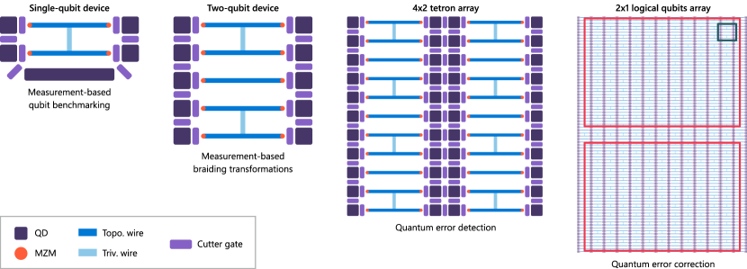
Figure 1: Roadmap to fault-tolerant quantum computation with tetrons. The first panel shows a single-qubit device. The tetron is formed through two parallel topological wires (blue) with a MZM at each end (orange dot) connected by a perpendicular trivial superconducting wire (light blue). The regions adjacent to the MZMs have quantum dots (QDs) shown in dark purple with cutter gates (light purple) controlling the tunnel coupling between the quantum dots and MZMs. The device supports measurement-based qubit benchmarking. The next panel shows a two-qubit device that supports measurement-based braiding transformations. The third panel shows a $4\times 2$ array of tetrons supporting a quantum error detection demonstration on two logical qubits. These demonstrations build towards quantum error correction, such as on the device shown in the right panel (a $27\times 13$ tetron array). The red boxes highlight the two fault-distance 7 logical qubits; the device is compatible with lattice surgery demonstrations. The blue-box highlights a two-qubit tile identical to the device in the second panel. Additional demonstrations may be inserted between the third and fourth panels to gradually scale the system.

Measurement-based topological qubits built upon Majorana zero modes (MZMs) stand out in this context as an architecture in which multi-qubit Pauli measurements are the native instruction set. This is unlike most conventional platforms, where these measurements are implemented by sequences of multi-qubit Clifford gates and single-qubit measurements. A specific MZM-based qubit architecture that enables such measurements was proposed in Refs. 3, 4, building on the ideas in Refs. 5, 6, 7 (see also Ref. 8). The qubits in this architecture are tetrons, which store the qubit state in four MZMs. The MZMs are located at the endpoints of two topological superconducting wires [9] formed from proximitized semiconductor nanowires [10, 11]. In this paper, we focus on two-sided tetrons, in which two parallel topological wires are joined by a trivial superconducting backbone to form a single island with charging energy [3]. In the remainder of this paper, we will drop the modifier and simply use tetrons to refer to two-sided tetrons. The measurements are performed by forming interferometric loops between qubit islands and nearby quantum dots, leading to a shift in the quantum capacitance of the dots that can be detected using standard microwave techniques. Such an interferometric parity measurement was recently demonstrated in Ref. 12 .

Tetrons are predicted to suppress idle and measurement errors exponentially in three dimensionless quantities: (i) the ratio of the topological gap to the temperature, (ii) the ratio of the length of the device to the topological superconducting coherence length, and (iii) the signal-to-noise ratio of the measurement system [14, 15, 16, 17, 18]. The resulting low error rates help enable scalable fault-tolerant quantum computation using recently introduced topological codes specifically tailored towards measurement-based qubits; see, e.g., Refs. 6, 19, 20, 21, 22. For a more detailed discussion of the practical advantages offered by this architecture for building a utility-scale fault-tolerant quantum computer, see the discussion in Sec. V.

We present a roadmap, summarized in Fig. 1, building towards fault tolerant quantum computing with tetrons. The roadmap incrementally scales the system while building the capabilities required for scalable quantum error correction. Sec. II describes the first device on the roadmap, a single topological qubit, with the ability to perform measurements in two different Pauli axes. This device can be used for measurement-based qubit benchmarking, the same method projected to benchmark tetrons in a scalable system. Sec. III describes the next step, a two-qubit device supporting single-qubit measurements in all Pauli axes as well as certain two-qubit measurements. The instruction set of this device supports a demonstration of entanglement and measurement-based braiding transformations [23, 3, 24], replacing older proposals for physically moving or adiabatically modifying tunnel couplings of the MZMs [25, 26, 27, 28, 29]. The subsequent milestone is the eight-qubit device described in Sec. IV, which supports multi-qubit Clifford gates and quantum error detection. We describe a specific quantum error detection scheme that uses the same measurements as those required for the syndrome extraction circuit of the Floquet codes in Refs. 20, 30, only a subset of which are needed for the pair-wise measurement-based surface code of Ref. 22. In Sec. V we discuss the outlook to these scalable quantum error correcting codes with the tetron architecture. An example device is the $2\times 1$ logical qubit array shown in the right-most panel of Fig. 1; each logical qubit (red box) supports the surface code with fault distance $7$. Additional details of the roadmap may be found in the appendices.

II Single-qubit tetron device

II.1 Measurement-based benchmarking of a topological qubit

For most conventional qubit platforms, coherent rotations are the elementary single-qubit operations, along with measurements in a distinguished “computational basis.” For measurement-based topological qubits, such rotations are only used to implement non-Clifford gates and, in a fault-tolerant setting, do not generally limit the system’s performance. Instead, topologically protected operations are performed through single- and two-qubit Pauli measurements. Notably, measurements, including two-qubit measurements, can be performed in several different axes without the need for unitary rotations . Therefore, the most natural way to validate such a qubit is through these Pauli measurements . In the single-qubit setting, this amounts to testing the ability to measure the qubit state in more than one Pauli basis.

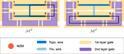
Figure 2: Gate schematic of the single-qubit device with measurement loops indicated. The tetron is formed by two parallel topological wires connected by a trivial superconducting backbone. MZMs form at each end of the topological wires and are labeled $1-4$ as shown. The chemical potential in the wires is controlled by first layer gates that deplete the 2DEG away from the superconductor. Quantum dot plungers and cutter gates between quantum dots and the MZMs are second layer gates. Depletion gates surround the device. The top and bottom panels show $X$ and $Z$ measurements formed by tuning the gates along the black lines and measuring on one of the quantum dot plunger gates involved in the loop.

It is worth noting that such non-commuting measurements have played an important role in the early development of quantum mechanics. The Stern-Gerlach experiment [33], which uses a magnetic field gradient to split a beam of spinful particles into two beams of well-defined spin orientation, was one of the first demonstrations of the discrete nature of quantum measurement outcomes. By combining two such Stern-Gerlach apparatuses with different orientation, one can probe the non-commutative nature of different spin observables. Here, we will describe a formally similar experiment, albeit in a completely different physical system, where the spin orientation is replaced by measuring different Majorana bilinears.

For an initial demonstration of a topological qubit, only two Pauli measurements, $X$ and $Z$ are needed. In the ideal case, these are projective measurements that anticommute exactly, $\{X,Z\}=0$. Therefore, for two subsequent $X$ measurements, the outcome of the second should be the same as the first, and likewise for two subsequent $Z$ measurements. In the Stern-Gerlach analogy, this corresponds to two sequential apparatuses having the same orientation, where the second does not split the individual beams any further. If, conversely, an $X$ measurement is followed by a $Z$ measurement (or vice versa $Z$ followed by $X$), the outcome of the second measurement should be equally distributed regardless of any previous measurement. In the Stern-Gerlach analogy, here the second apparatus has a different orientation and is able to split each output beam of the first one in half again. Performing a sequence of $X$ and $Z$ measurements and statistically analyzing the outcomes allows us to infer whether they indeed correspond to two anticommuting, projective measurements, within some well-defined approximation. We propose a number of such statistical tests, which we refer to collectively as measurement-based qubit benchmarking (MBQB) . Similar tests were proposed and experimentally performed on nuclear spin qubits in Ref. 35. Importantly, these protocols test not only the accuracy of the classical outcomes reported by the measurements, but also the quality of the post-measurement quantum state .

To quantify deviations from the ideal case, we introduce two operational error metrics: the operational assignment error ${\sf{err}_{a}}$  and the operational bias ${\sf{err}_{b}}$. The former is the deviation of the experimental $X$ and $Z$ measurements from their ideal projective behavior, quantified by the total variational distance between the observed and expected outcome statistics maximized over different preparations and bases. More explicitly, writing ${\mathcal{M}^{P}_{r}}$ to be the superoperator corresponding to the (generally imperfect) implementation of the measurement of the Pauli operator $P$ with outcome $r\in\{+1,-1\}$, then 

$${\sf{err}_{a}} =\max_{s,P}\frac{1}{2}\sum_{r}\left|\Pr\left({\mathcal{M}^{P}_{r}}\Big{|}{\mathcal{M}^{P}_{s}};\frac{1}{2}\tilde{\openone}\right)-\delta_{r,s}\right|$$ (1)

$$=\max_{s,P}\left|\Pr\left({\mathcal{M}^{P}_{+1}}\Big{|}{\mathcal{M}^{P}_{s}};\frac{1}{2}\tilde{\openone}\right)-\delta_{+1,s}\right|,$$ (2)

where $\frac{1}{2}\tilde{\openone}$ is an experimental approximation to the maximally mixed state. We have written the conditional probability of getting outcome $r$ immediately after outcome $s$ having prepared the initial state $\frac{1}{2}\tilde{\openone}$ as $\Pr\left({\mathcal{M}^{X}_{r}}\Big{|}{\mathcal{M}^{X}_{s}};\frac{1}{2}\tilde{\openone}\right)$.

The operational bias error quantifies the deviation from the mutually unbiased bases behavior of $X$ and $Z$ measurements [39, 40]. For a single-qubit, this means that an $X$ measurement after a $Z$ measurement should yield either outcome with probability $1/2$. As such, the operational bias corresponds to maximizing the total variation distance over sequences of pairs of nominally distinct measurements:

$${\sf{err}_{b}} =\max_{s,P\neq Q}\frac{1}{2}\sum_{r}\left|\Pr\left({\mathcal{M}^{P}_{r}}\Big{|}{\mathcal{M}^{Q}_{s}};\frac{1}{2}\tilde{\openone}\right)-\frac{1}{2}\right|$$ (3)

$$=\max_{s,P\neq Q}\left|\Pr\left({\mathcal{M}^{P}_{+1}}\Big{|}{\mathcal{M}^{Q}_{s}};\frac{1}{2}\tilde{\openone}\right)-\frac{1}{2}\right|.$$ (4)

Together, ${\sf{err}_{a}}$ and ${\sf{err}_{b}}$ inform not only how distinguishable the experiments are from the ideal behavior, but also what aspect of the experiment deviates the most. Further details of these operational error metrics are discussed in Sec.Sec. A, including how the experiments used to estimate them can be used to reconstruct the full action of the measurements on a quantum state.

It is worth considering some concrete examples of non-ideal behavior. If the measurement operations yield uniformly random outcomes, such as in the case where switching the measurement on and off completely randomizes the state of the qubit, ${\sf{err}_{a}}=1/2$ and ${\sf{err}_{b}}=0$. On the other hand, if the quantum device is able to implement the measurement projector perfectly but noise in the readout chain, e.g., due to the amplifiers, flips the recorded measurement with probability $p_{f}$, one would find ${\sf{err}_{a}}=2p_{f}(1-p_{f})$ and ${\sf{err}_{b}}=0$. Finally, if both measurements are actually identical instead of anticommuting, but otherwise perfect, then ${\sf{err}_{a}}=0$ and ${\sf{err}_{b}}=\frac{1}{2}$.

The experiments implied by the definition of the ${\sf{err}_{a}}$ and ${\sf{err}_{b}}$ metrics assume the ability to prepare $\frac{1}{2}\tilde{\openone}$, an approximation to the maximally mixed state. In practice, the maximally mixed state can be approximated by applying a sequence of approximately non-commuting measurements without conditioning on the outcomes. Estimating ${\sf{err}_{a}}$ and ${\sf{err}_{b}}$ then requires estimating the probability of subsequences

$${\mathcal{M}^{P}_{r}}{\mathcal{M}^{Q}_{s}} {\mathcal{M}^{R}_{*}}{\mathcal{M}^{S}_{*}}, {\mathcal{M}^{P}_{r}}{\mathcal{M}^{P}_{s}} {\mathcal{M}^{R}_{*}}{\mathcal{M}^{S}_{*}},$$ (5)

where $P\neq Q,R\neq S\in\{X,Z\}$ and the $*$ indicates that we do not care about that particular measurement outcome. One can then imagine running an experiment consisting of a long random or pseudorandom sequence of measurements and counting the separate occurrence frequencies of Eq. 5 as subsequences, see Sec.Sec. A.

While the above definitions could be generalized to include $Y$ measurements, initial demonstrations of topological qubits will be restricted to use $X$ and $Z$ measurements for simplicity of device control, as shown in Fig. 2. Under these restrictions, only the real part of the states and transformation can be fully reconstructed, but that suffices for the reconstruction of the action of $X$ and $Z$ measurements and for the definition of the natural error metrics introduced above (see Sec.Sec. A for more details). MBQB can be generalized in other ways. For instance, the measurement sequence could include experimentally distinct implementations of the $X$ and $Z$ measurements (e.g., sometimes measuring $X$ using $i\gamma_{1}\gamma_{3}$ and sometimes measuring $X$ using $i\gamma_{2}\gamma_{4}$, which is equivalent in the computational subspace). It is also possible to include two-qubit measurements in the sequence.

MBQB allows us to extract operational error metrics for a qubit assuming only the ability to perform sequences comprising two non-commuting Pauli measurements. However, at least one unitary outside the Clifford group is needed to perform universal quantum computation [41]. A $\pi/4$ rotation around $Z$, known as the $T$ gate, is often chosen as the operation to complete a universal set of gates, but this is not a topologically-protected operation in Majorana-based qubits. However, a noisy implementation of the $T$ gate together with low-noise Clifford operations can be used to distill low noise resource states from which fault-tolerant $T$ gates can be implemented [42, 43]. The required Clifford operations can be performed through topologically protected single- and two-qubit measurements, as described in Sec. III.1.

II.2 Device design

II.2.1 Design elements

Fig. 2 shows a gate schematic of the two-sided tetron. The principal elements of the design are: (1) two parallel topological superconducting nanowires (blue), with MZMs at their ends (orange dots); (2) a trivial superconducting nanowire that connects the midpoints of the topological wires (light blue), so that the three wires together form a (sideways) ‘H’; (3) five quantum dots; (4) tunnel junctions coupling these quantum dots to each other as well as to the MZMs. As in the case of the linear tetron device described in Ref. 12 (as well as the devices of Refs. 44, 45, 46), the nanowires are gate-defined and can be realized in a material stack featuring a two-dimensional electron gas (2DEG) formed in an InAs quantum well that is proximitized by an epitaxially-grown $s$-wave superconductor such as Al. The most crucial differences between the two-sided design and the linear tetron device described in Ref. 12 are that the topological superconducting segments are no longer colinear and the trivial superconducting segment, which is perpendicular to them, remains far from the MZMs. The placement of MZMs at the four corners of the H is advantageous for multi-qubit layouts with 2D connectivity. As the qubit islands are floating, a complete theoretical treatment of their ground state degeneracy requires a number-conserving formalism, as discussed in Refs. [5, 47, 17, 24].

The “horizontal” topological superconducting wires can be gate-defined as follows. Each “horizontal” superconducting strip can be covered by a “plunger” gate that is used to tune the density of electrons in the semiconductor under the corresponding superconducting wire. The wires are narrow enough that the semiconductor can be tuned into the single-subband regime [46], and their length is chosen to minimize residual coupling between the Majorana zero modes while still supporting sufficient charging energy. For material stacks similar to the one used in Ref. 12, a length of $35\text{\,}\mathrm{\SIUnitSymbolMicro m}$ meets these criteria. Under normal operating conditions, there is an in-plane magnetic field of several Teslas in the “horizontal” direction, i.e., along the topological wires. The material stack and device can be designed [48, 49] so that there is a range of in-plane magnetic fields and plunger gate voltages (within the lowest sub-band) over which both of the horizontal wires are in the topological phase with MZMs at the ends, provided disorder is sufficiently low [50, 51, 52, 53, 54, 55, 56, 57, 58, 59, 60, 61, 62, 63, 64, 65, 66, 67]. The “vertical” trivial superconducting wire connects the topological segments (the cross-bar of the H) and needs to be engineered in such a way that it does not introduce low-energy subgap states. The distance between the horizontal wires is approximately $1\text{\,}\mathrm{\SIUnitSymbolMicro m}$, dictated by requirements on the quantum dots discussed below.

There is a quantum dot adjacent to each endpoint of the horizontal wires and, thus, to the MZM that resides there. There is also a longer quantum dot parallel to the bottom wire that enables connections between the left and the right side of the device. These quantum dots have a form and function similar to those of the device used in Ref. 12, with the extended dot mirroring the dimensions of the extended dots on the linear tetron device, and the dots adjacent to the bottom wire extended somewhat to connect with the long quantum dot. All the dots can be designed so that their charging energies and level spacings are large compared to the electronic temperature. Unlike in the linear tetron device, the junctions connecting these quantum dots to the topological superconducting wires are at the ends of the wires.

Related methods for parity measurement were discussed in Refs. 68, 69, 70, 71, 72, 73, 6, 4, 7, 74, 75, 76, 77, 78. Analogous device architectures might apply to other physical systems that have been proposed for MZMs, including quasi-one-dimensional systems composed of chains of magnetic atoms on the surface of a superconductor [79, 80, 81, 82, 83, 84]; in nanowires that are completely encircled by a superconducting shell in which the order parameter winds around the wire due to the orbital effect of the magnetic field [85, 86, 87]; in the vortex cores of three-dimensional superconductors [88, 89]; in two-dimensional $p+ip$ superconductors [90]; at the surface of a topological insulator [91, 92, 93]; in ferromagnetic insulator-semiconductor-superconductor heterostructures [94, 95, 96, 97, 98, 99, 100, 101]; in $s$-wave superfluids of ultra-cold fermionic atoms [102, 103]; and potential non-Abelian fractional quantum Hall states [104, 105, 106, 107]. In the latter system, interferometric transport measurements of fermion parity were proposed in Refs. 108, 109, 110, 111, and intriguing results have been observed in experiments [112, 113].

II.2.2 Operating principles and dominant error sources

The quantum state of a tetron is encoded in four Majorana zero modes (MZMs), which can be numbered as shown in Fig. 2. Assuming a fixed MZM parity $-\gamma_{1}\gamma_{2}\gamma_{3}\gamma_{4}=+1$, we can define Pauli operators .

$$Z =i\gamma_{1}\gamma_{2}=i\gamma_{3}\gamma_{4}$$ (6)

$$X =i\gamma_{1}\gamma_{3}=-i\gamma_{2}\gamma_{4}.$$ (7)

Since topological qubits have near-degenerate ground states, there is no preferred “computational basis“, and the assignment of Pauli operators above is purely a matter of convenience. With the choice made above, the basis states of the qubit can be chosen as the eigenstates of the $Z$ operator, i.e. $Z|0\rangle=+|0\rangle$ and $Z|1\rangle=-|1\rangle$.

The primary operations supported by the single-qubit device are measurements in $X$ and $Z$, performed by forming interferometric loops as indicated in Fig. 2. By enabling single-electron tunneling between the Majorana zero modes and an adjacent chain of quantum dots, a state-dependent shift of the energy spectrum of the quantum dots is induced. This shift can be measured as a change in the capacitance of a nearby gate to the quantum dot (referred to as quantum capacitance), which in turn is detected as a frequency shift of a microwave resonator that is coupled to that gate. This approach is explained in more detail in Refs. 115 and has been experimentally demonstrated in Ref. 12. Qubit states are prepared using such measurements, which need to be followed either by post-selection, a Clifford operation to correct the outcome, or classical tracking of the Pauli reference frame; in practice, the latter approach is usually favorable (see Sec. III.1). Qubit states can be transformed into each other using the approaches discussed in Sec. III.1.

While topological qubits are affected by errors due to imperfect control, coupling to the environment, and inherent physical limitations, their topological protection suppresses these errors exponentially in the dimensionless quantities discussed in Sec. I. These errors can be separated into classical errors that flip the measurement outcomes, and quantum errors that couple to the MZMs. The former are limited by the signal-to-noise ratio (SNR), and occur with probability 

$$p_{a} =\left[1-\text{erf}\left(\frac{\text{SNR}(\tau_{\text{meas}})}{\sqrt{2}}\right)\right]/2.$$ (8)

Typically, $\text{SNR}(\tau_{\text{meas}})\sim\sqrt{\tau_{\text{meas}}}$ for sufficiently long measurement times, and $\lim_{x\to\infty}\left[1-\text{erf}(x)\right]\sim e^{-x^{2}}/x$, thus the probability decays exponentially with increasing $\tau_{\text{meas}}$. The interferometric parity measurement proposed here was demonstrated in Ref. 12, where an SNR of $0.52$ was achieved for a measurement time of $1\text{\,}\mathrm{\SIUnitSymbolMicro s}$. We comment on future improvements to the SNR in Sec. V.

Errors on the quantum state, on the other hand, become more likely when the measurement time is increased because the qubit state may change during the measurement. The typical timescale for undesired changes of the quantum state is denoted by $T_{\text{life}}$. The resulting error probability during a measurement is expected to scale as

$$p_{1} \sim 1-e^{-\tau_{\text{meas}}/T_{\text{life}}}.$$ (9)

While in conventional qubits, $T_{\text{life}}$ is governed by relaxation into the lower-energy state and typically denoted by $T_{1}$, in topological qubits, there is no strongly preferred basis and $T_{\text{life}}$ will have contributions from processes other than relaxation. The processes predominantly limiting $T_{\text{life}}$ are due to (i) thermal fluctuations exciting a fermion from the MZMs to an above-gap quasiparticle state (scaling as $e^{-\Delta/k_{B}T}$)  and (ii) state flips due to the residual coupling between a MZM involved in a measurement and a MZM not involved in a measurement. Both errors can be modeled phenomenologically as Pauli errors, see Appendix B for details .

To perform an $X$ (or $Z$) measurement, the quantum dots that lie on the $X$ ($Z$) loop must be coupled to the qubit island while those on the $Z$ ($X$) loop must be decoupled from the island. In an MBQB demonstration, the device must switch between these two configurations. This can be done by coupling/decoupling quantum dots from the qubit island in one of two ways. The “detuning-based” approach decouples a dot from the qubit island and other dots by setting its chemical potential to lie in a Coulomb valley. We couple a dot to the qubit island by tuning it near its charge degeneracy point (which also couples it to other dots that are near their charge degeneracy points). Alternatively, the “cutter-based” approach additionally uses a cutter gate to open or close a junction, thereby decoupling a dot on one side of the junction from the qubit island (or dot) on the other side of the junction.

The detuning-based approach uses small amplitude pulses on the plunger gates (or equivalently on any gate with significant lever arm to the quantum dot of interest and small lever arm to other regions). However, in this approach, the coupling through the $X$ ($Z$) loop is only suppressed by a factor $\sim t^{2}/E_{C}^{\text{QD}}$ during the $Z$ ($X$) measurement, where $t$ is the tunnel coupling between dots or dot and wire and $E_{C}^{\text{QD}}$ is the QD charging energy. This residual coupling limits $T_{\text{life}}$ because the unwanted coupling fluctuates as a result of charge noise, thereby decohering the qubit. With cutter-based control, the residual coupling can be made exponentially small in the width of the tunnel barrier , so qubit coherence is limited instead by the residual coupling of the MZMs through the qubit island. This scales as $e^{-L/\xi}$ where $L$ is the length of the topological wires and $\xi$ is the superconducting coherence length in the topological phase. Note that a $Y$ measurement in the device shown in Fig. 2, e.g., $i\gamma_{1}\gamma_{4}$, requires cutter-based control as the $Z$ and $X$ loops are only closed off by the cutter adjacent to MZM $\gamma_{3}$.

III Measurement-based braiding transformations

Unitary gate operations can be performed via measurements with the aid of auxiliary degrees of freedom [120, 121]. Such measurement-based operations on topological qubits, pioneered in Ref. 23, preserve topological protection, while removing the need to physically move anyons. In the case of tetrons, Clifford operations are topologically protected and can be enacted entirely through single-qubit and two-qubit (2-MZM and 4-MZM) measurements involving auxiliary tetrons. For example, to perform a full set of single-qubit Clifford operations, a system of two qubits is required, where one serves as the computational qubit and one as an auxiliary qubit. In this section, we will describe the corresponding measurement sequences for such measurement-based single-qubit Clifford operations and introduce a design for a device that is able to execute them.

It is worth noting that performing Clifford gates directly on physical qubits is not necessary for scalable quantum computation in the architecture described in this paper. Instead, Clifford gates are performed directly on logical qubits through so-called lattice surgery operations (see also the discussion in Sec. IV), and the only required physical operations are the measurements needed to perform error correction and the $T$ gate to achieve universality. Nevertheless, performing such Clifford gates via measurement-based braiding transformations is an important step on this roadmap as it implies a powerful demonstration of the non-Abelian nature of MZMs . While these Clifford gates allow for a comparison to conventional qubit platforms, a more natural comparison is the fidelity of operations used in a quantum error correction syndrome extraction circuit, which in our architecture are the Pauli measurements themselves, and in other platforms include the Clifford gates.

As the measurements involved are topological, the operations generated by these measurement sequences directly reflect the fusion and braiding statistics of the corresponding topological phase [23]. However, the charging energy of a superconducting island fixes the total fermion parity of the four MZMs on each tetron, so we can only perform operations that preserve this parity [3, 24]. Equivalently, all measurements must involve an even number of Majorana operators on each island. This is sufficient to generate a complete set of Clifford gates.

We note also that this approach can be extended to multi-qubit Clifford operations; for a more complete discussion, see Refs. 3, 123. On the other hand, going beyond Clifford operations to obtain a computationally universal gate set requires additional, non-topologically-protected operations. Such operations, which are discussed in, for instance, Refs. 124, 125, are not the focus of this paper.

III.1 Protocols

An ideal measurement of two-qubit Pauli $PQ$ with outcome $s\in\{\pm 1\}$ corresponds to the projector

$${{\Pi}^{PQ}_{s}} =\frac{\openone+s\cdot PQ}{2}.$$ (10)

Using this, one can verify that the phase gate $S$ applied to the computational qubit can be generated, up to a Pauli correction , by the sequences of four measurements shown in Fig. 3: ${\mathcal{M}^{XI}}{\mathcal{M}^{YI}}{\mathcal{M}^{ZZ}}{\mathcal{M}^{XI}}$. (Here, the sequence of measurements is to be read right to left, like operators applied to a state.) In particular, we find

$${{\Pi}^{XI}_{s_{3}}}{{\Pi}^{YI}_{s_{2}}}{{\Pi}^{ZZ}_{s_{1}}}{{\Pi}^{XI}_{s_{0}}} =\mathcal{O}^{s_{0}}_{s_{3}}\otimes Z^{\frac{1+s_{0}s_{1}s_{2}}{2}}S,$$ (11)

where the operator $\mathcal{O}^{s_{0}}_{s_{3}}$ on the auxiliary qubit is a shorthand for $|X_{s_{3}}\rangle\langle X_{s_{0}}|$. (The equivalence in Eq. (11) is up to overall constants, which are unimportant for the effective operations generated.) The diagrammatic representation of this measurement sequence, shown in Appendix C, illuminates the relation to the corresponding braiding transformation. We note that this measurement sequence requires only a single two-qubit measurement. Furthermore, the first and last measurement in the sequence initialize and reset the auxiliary qubit in the $X$ basis, and therefore one of them could potentially be omitted in a series of gate operations, though this comes with the potential risk of propagation of errors between subsequent Clifford operations. Finally, this measurement sequence is not unique; in general, many different sequences can be used to generate a given Clifford gate. The optimal choice of sequence will depend on the details of the underlying hardware implementation. Here, we have chosen sequences that are well-suited to the qubit design described below in Sec. III.2; for a broader discussion of this optimization, see Ref. 123.

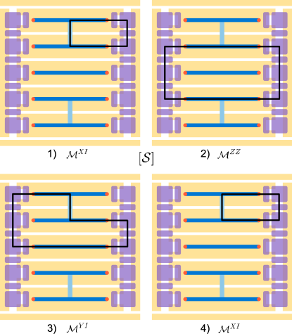
Figure 3: Measurement sequence for implementing $[{\mathcal{S}}]$ in Eq. 13 on the two-qubit device (same legend as in Fig. 2). The sequence is equivalent to applying a braid to MZMs $1$ and $2$ on the computational (bottom) qubit, see Sec.Sec. C for the explicit connection.

We note that the Pauli correction arising from the measurement sequence in Eq. 11 (or from similar operator-generating measurement sequences) is not deterministic, since the measurement outcomes are probabilistic. In principle, these outcomes can be made deterministic by employing a repeat-until-success protocol called “forced measurement” [23, 123], where measurements in the sequence are replaced by (longer) adaptive measurement sequences. However, this is not necessary: instead, the Pauli corrections can be tracked in software, where they lead to a classical correction of the final measurement outcome or potentially a modification of subsequent non-Clifford operations. Therefore, it is convenient to work directly with the Pauli equivalence class $[C]$ of a Clifford gate $C$, defined as $[C]=\{C^{\prime}\in\mathfrak{C}|\exists P:PC^{\prime}=C\}$, where $\mathfrak{C}$ is the Clifford group of unitaries acting on a single qubit, and $P$ is a Pauli operator. Any given element of the equivalence class can be accessed through changes to the Pauli frame [127], without any additional operations on the qubits themselves.

While the single-qubit Clifford group has 24 elements, there are only 6 Pauli equivalence classes, which we denote $[\openone]$, $[H]$, $[S]$, $[HSH]$, $[HS]$, and $[SH]$. For the two-qubit device described in the next section, examples of optimized measurement sequences for the nontrivial Pauli equivalence classes of single-qubit Clifford gates are

$$[{\mathcal{H}}] ={\mathcal{M}^{XI}}{\mathcal{M}^{YI}}{\mathcal{M}^{ZY}}{\mathcal{M}^{XI}},$$ (12)

$$[{\mathcal{S}}] ={\mathcal{M}^{XI}}{\mathcal{M}^{YI}}{\mathcal{M}^{ZZ}}{\mathcal{M}^{XI}},$$ (13)

$$[{\mathcal{HSH}}] ={\mathcal{M}^{XI}}{\mathcal{M}^{ZY}}{\mathcal{M}^{ZZ}}{\mathcal{M}^{XI}},$$ (14)

$$[{\mathcal{SH}}] ={\mathcal{M}^{XI}}{\mathcal{M}^{YI}}{\mathcal{M}^{ZY}}{\mathcal{M}^{ZZ}}{\mathcal{M}^{XI}},$$ (15)

$$[{\mathcal{HS}}] ={\mathcal{M}^{XI}}{\mathcal{M}^{YI}}{\mathcal{M}^{ZZ}}{\mathcal{M}^{ZY}}{\mathcal{M}^{XI}}.$$ (16)

Here we use ${\mathcal{C}}$ to represent the superoperator corresponding to the unitary $C$, and use ${\mathcal{M}^{P}}$ to represent the instrument used to measure the observable $P$. The corresponding Pauli corrections are elided for brevity, but can be efficiently computed (see Appendix C).

To experimentally validate successful execution of such measurement-based protocols, we can tomographically reconstruct the action of each of the measurement sequences on the computational qubit. The impact of state preparation and measurement (SPAM) errors can be separated and accounted for through reference experiments, and the most robust way to do so is through gate-set tomography [128]. To this end, we prepare the computational qubit in the eigenstate of a Pauli operator via measurement, and characterize the final state in the Pauli basis, leading to the nine inequivalent sequences 

$${\mathcal{M}^{IX}}[\mathcal{C}]{\mathcal{M}^{IX}} {\mathcal{M}^{IY}}[\mathcal{C}]{\mathcal{M}^{IX}} {\mathcal{M}^{IZ}}[\mathcal{C}]{\mathcal{M}^{IX}}$$ , , , (17a)

$${\mathcal{M}^{IX}}[\mathcal{C}]{\mathcal{M}^{IY}} {\mathcal{M}^{IY}}[\mathcal{C}]{\mathcal{M}^{IY}} {\mathcal{M}^{IZ}}[\mathcal{C}]{\mathcal{M}^{IY}}$$ , , , (17b)

$${\mathcal{M}^{IX}}[\mathcal{C}]{\mathcal{M}^{IZ}} {\mathcal{M}^{IY}}[\mathcal{C}]{\mathcal{M}^{IZ}} {\mathcal{M}^{IZ}}[\mathcal{C}]{\mathcal{M}^{IZ}}$$ , , . (17c)

The reference experiments correspond to similar experiments replacing $[\mathcal{C}]$ with a trivial operation, resulting in the additional nine sequences

$${\mathcal{M}^{IX}}{\mathcal{M}^{IX}} {\mathcal{M}^{IY}}{\mathcal{M}^{IX}} {\mathcal{M}^{IZ}}{\mathcal{M}^{IX}}$$ , , , (18a)

$${\mathcal{M}^{IX}}{\mathcal{M}^{IY}} {\mathcal{M}^{IY}}{\mathcal{M}^{IY}} {\mathcal{M}^{IZ}}{\mathcal{M}^{IY}}$$ , , , (18b)

$${\mathcal{M}^{IX}}{\mathcal{M}^{IZ}} {\mathcal{M}^{IY}}{\mathcal{M}^{IZ}} {\mathcal{M}^{IZ}}{\mathcal{M}^{IZ}}$$ , , . (18c)

In its simplest form, the gate set tomography procedure solves a linear problem to obtain a superoperator representation ${\mathcal{C}}$, including imperfections due to noise, implementation imperfections, and finite statistics. Error metrics such as gate fidelity can be directly extracted by comparing ${\mathcal{C}}$ to the ideal superoperator. It is worth noting that such metrics for the execution of unitary gates allow a direct comparison to more conventional qubit platforms.

III.2 Two-qubit device design

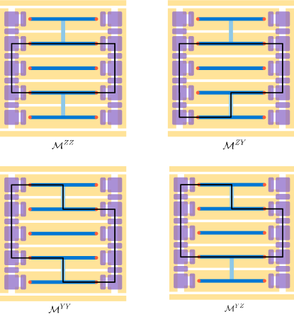
Figure 4: Two-qubit measurement loops supported on the two-qubit device, with the same legend as in Fig. 2.

The two-qubit device supporting a measurement-based braiding demonstration builds off the single-qubit device described in the previous section. Two tetrons are stacked vertically, such that the device supports all single-qubit Pauli measurements and the two-qubit measurements: ${\mathcal{M}^{ZZ}},{\mathcal{M}^{YY}},{\mathcal{M}^{YZ}},{\mathcal{M}^{ZY}}$. A device schematic with these two-qubit loops is shown in Fig. 4.

A key design change is that the longer quantum dot of the single-qubit device is replaced by a coherent link (floating topological wire), which is situated between the two tetrons. This component is used to facilitate measurements involving MZMs on opposite sides of a tetron (i.e., single qubit $Z$ and $Y$ measurements). For the long quantum dot, the relevant energy scale to low-lying excitations is the level spacing, which decreases with length; for the coherent link, on the other hand, the relevant scale is the topological gap. Therefore, switching to a coherent link facilitates using longer topological wires and thus achieving smaller MZM energy splitting through the topological wires of the qubits, which helps increase qubit lifetime.

Two-qubit measurements introduce the potential for correlated two-qubit errors. Such errors can occur from, e.g., tetrons exchanging an electron through the MZMs during the measurement, such that the final charge states of the qubit islands have changed before and after the measurement. These two-qubit state errors can also be modeled as Pauli errors, see Sec.Sec. B for details .

IV Quantum error detection in a $4\times 2$ array of tetrons

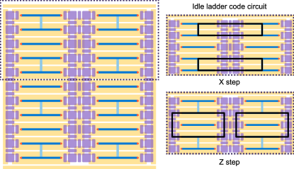
Figure 5: Left panel. Gate schematic for a $4\times 2$ qubit array following the same legend as in Fig. 2. The two columns of qubits are connected by a double-rail of quantum dots separated by depletion gates and a dot cutter. Right panel. Syndrome extraction circuit for the idle ladder code: the $X$ step is alternated with the $Z$ step as shown; after each step the instantaneous stabilizer group corresponds to the two-qubit measurements that were just performed, as well as the product $YYYY$ on the four qubits, inferred from the measurement outcomes of the previous two steps.

IV.1 Overview

Fault-tolerant quantum error correction [131, 132, 133, 134, 135, 136, 137] is a crucial ingredient for any scalable quantum computing platform. Recently, the field of quantum error correction has advanced drastically from demonstrations with encoded states (and no repeated error correction) [138, 139, 140, 141, 142, 143] to successful demonstrations of repeated error correction across several platforms. In ion traps, both repeated error detection [144, 145], error correction [146, 147, 148], and error corrected computation [149] have been performed—in some notable cases demonstrating logical error rates below the corresponding physical error rates [148, 149]. In superconducting qubits, recent progress on repeated error detection and correction [150, 151, 152, 153, 154, 155, 156] has culminated in a demonstration of sub-threshold error correction in the surface code [157, 158] and the color code (including logical operations) [159].

For tetron qubits, a very natural class of codes are the Hastings-Haah Floquet codes [20, 160, 161, 162, 30]. These codes are closely related to the surface code, but rely entirely on one- and two-body measurements to extract error syndromes, making them very naturally well suited to the capabilities of the tetron platform. Within the class of Floquet codes, the ladder code is an intriguing first demonstration, as it uses few qubits but builds on the same set of two-qubit measurements as the scalable Hastings-Haah Floquet codes and thus falls naturally on a roadmap towards scalable quantum computation.

To demonstrate a non-trivial improvement of system performance, it is important to go beyond idle operation of such a code to demonstrate a logical operation between two qubits. A promising way to perform such logical operations at scale is lattice surgery [163]: here, two logical qubit patches are stitched together to form a single, larger patch, which effectively performs a two-logical-qubit measurement. In a later step, the enlarged patch is split back into two separate logical qubits. Leveraging these two-qubit measurements, logical Clifford gates can be performed in a way that is conceptually very similar to the measurement-based braiding transformations discussed in Sec. III.1. Surgery is generally accomplished by turning on additional stabilizer measurements connecting the boundaries of the two code patches, with details depending strongly on the specific code and circuit realization being used. As we discuss below, such a surgery operation is particularly simple to implement in the ladder code being used here. The logical two-qubit measurement performance obtained through this scheme can be compared to the physical two-qubit measurement performance by extracting the logical error per round from a repetition code decay experiment. Demonstrating logical improvement for a two-qubit measurement is a key advance on the path to scalable fault-tolerant quantum computation with Majorana-based qubits, as it directly compares the native operation of the physical qubits with the corresponding operation of the logical qubits.

IV.2 Ladder code

The ladder code can be defined on an array of $N\times 2$ tetrons ($N>1$), and relies on $XX$ measurements between the columns as well as $YY$ and $ZZ$ measurements between rows of qubits. Similar to the repetition code, its logical operators are highly asymmetric in weight; therefore, for sufficiently large $N$, it is able to correct errors in one basis but not the other . For $N=2$, the ladder code is equivalent to the $d=2$ Bacon-Shor error detecting code [165, 166]. It is important to note that due to the structure of the circuits used to perform error detection, some elementary faults, such as correlated two-qubit errors occurring during a single two-qubit measurement, will remain undetected.

The idle ladder code circuit on a $2\times 2$ array of qubits has two steps shown in the right panel of Fig. 5: in the first step an $XX$ measurement is performed on the two pairs of horizontal nearest neighbor qubits, while in the second step a $ZZ$ measurement is performed between the two pairs of vertical nearest neighbor qubits. Let $\overline{P}$ denote the logical Pauli $P$ of the ladder code. The logical group generators are $\overline{Z}=ZZ$ between horizontal nearest neighbor qubits and $\overline{X}=XX$ between vertical nearest neighbor qubits. The instantaneous stabilizer group after a given step corresponds to the product of $Y$ on all four qubits as well as the two-qubit measurements performed at that step; any change in the stabilizer outcome indicates an error has occurred.

Figure 6: The four steps of the $\overline{ZZ}$ measurement circuit for the ladder code (same legend as in Fig. 2). The $\overline{ZZ}$ measurement outcome is inferred after steps 4 and 1 (assuming at least one previous round of the circuit).

The eight-qubit $4\times 2$ device required for the lattice surgery demonstration has two of the logical qubits described above stacked vertically. A $\overline{ZZ}$ measurement on the two logical qubits is performed by the circuit shown in Fig. 6. The $X$ and $Z$ steps of the idle circuit are performed, followed by an additional $X$ step and then a new $Y$ step entangling the two logical qubits. The instantaneous stabilizer group after a given step is given by the two-qubit measurements performed in that step, and additionally each logical qubit’s $YYYY$ stabilizer after steps 2 and 3, and $\overline{ZZ}$ after steps 1 and 4. Again, any change in the stabilizer outcomes indicates an error has occurred.

IV.3 Decay experiment and simulations

To compare the $\overline{ZZ}$ measurement on the logical qubits to a $ZZ$ measurement on a pair of physical qubits, we compare the repetition code run directly on the physical qubits with the repetition code concatenated with the ladder code. Specifically, we envision the following decay experiment: (1) initialize the qubits (logical or physical) in a logical state of the repetition code; (2) perform $N$ repetitions of the (logical or physical) $ZZ$ measurement circuit, corresponding to error detection cycles for the repetition code; (3) characterize the final state to identify undetected faults. For both the logical and physical qubit case, post-select on runs for which no errors are detected, i.e., for which the stabilizer outcomes are unchanged. The decay experiment is repeated for different initial logical states, which can be used to characterize the decay of the repetition code logical operators $\widetilde{X}=XX$ and $\widetilde{Z}={ZI}$. Due to the inherent asymmetry of the repetition code, the associated decay rates can behave qualitatively differently. Details of this are discussed in Sec.Sec. D. Defining the decay rate of Pauli $P$ as $\lambda_{P}$, we characterize the performance through the average logical improvement $\Lambda$

$$\Lambda =\frac{\lambda_{XX}+\lambda_{ZI}}{\lambda_{\overline{XX}}+\lambda_{\overline{ZI}}},$$ (19)

i.e., the ratio of the average decay rate for the physical circuit to the average decay rate for the logical circuit.

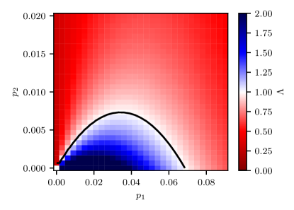
Figure 7: Average logical improvement $\Lambda$ (Eq. 19) for the $ZZ$ measurement, plotted as a function of single-qubit Pauli error probability $p_{1}$ and two-qubit Pauli error probability $p_{2}$ for assignment error $p_{a}=0.01$. The blue region bounded by the black curves shows parameter values for which logical improvement is expected.

The decay rates (equivalently, logical errors per round) are extracted by varying the number of rounds $N$ and fitting the results to an exponential for both the logical and physical circuit. We simulate this decay experiment for an effective noise model in which single-qubit Pauli errors occur with probability $p_{1}$, two-qubit Pauli errors occur with probability $p_{2}$ and classical assignment errors occur with probability $p_{a}$ (see Sec.Sec. B for additional details). Defining the average logical improvement according to Eq. 19, we extract the parameter space for which quantum error detection shows logical improvement of the $ZZ$ measurement, shown by the black curve in Fig. 7. Note there is an optimal single-qubit Pauli error probability that maximizes the allowed two-qubit Pauli error probability for which there is still logical improvement. Furthermore, there is generally no improvement if $p_{1}=p_{2}=p$, which is to be expected since these circuits are not fault-tolerant for circuit-level noise. However, in practice we expect $p_{2}<p_{1}$ for tetron qubits, see discussion in Appendix B.

V Outlook: scalable quantum error correction schemes

The roadmap outlined above builds towards scalable quantum error correction with tetrons. Most importantly, the basic qubit design and functionality is unchanged after the two-qubit device, up to optimizations of the component dimensions. The operations required for error correction in the Hastings-Haah Floquet codes [20, 30] or the pair-wise measurement-based surface code [22] are a subset of the measurements used in the three demonstrations described above; no additional qubit capabilities are required. In particular, the syndrome extraction circuit for the Hastings-Haah Floquet codes use exactly the same set of two-qubit measurements as for the quantum error detection demonstration. Finally, each successive milestone described in the above roadmap requires improved physical qubit performance while increasing the scale of the system, the same two axes along which we must progress to achieve scalable quantum error correction. Demonstrating successive milestones both de-risks our understanding of the errors affecting tetrons and indicates the path forward.

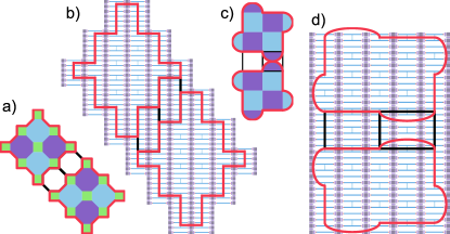
Figure 8: A device with two logical qubits with fault distance $3$ encoded in the 4.8.8 Hastings-Haah code [20, 30] (a, b) and the 3 aux surface code (c, d) [22]. The colored faces indicate how the syndrome extraction circuits are constructed, and how the corresponding plaquettes map to a tetron array. Throughout, a thick, red line highlights the region representing a single logical qubit. Black lines outline regions used to perform lattice surgery between the patches.

For the code distances required for utility scale quantum computing, inevitably we will run into instances of physical qubit failure. While early devices can require all qubits to be functional and within specification, scalable systems will require implementing vacancy mitigation strategies in the syndrome extraction circuit. Vacancy mitigation for the Hastings-Haah Floquet codes and pair-wise measurement-based surface code was described in Refs. 22, 167. Demonstrating these circuits in an actual device require logical qubit patches with fault distance of at least 5 so that error correction is still possible in the presence of a sparse number of failed components.

A demonstration of scalable quantum error correction with tetrons should support both idle and logical operations below the code threshold, and utilize the vacancy mitigation in the syndrome extraction circuits [167, 22]. As such, we propose a tetron array supporting $2\times 1$ logical qubits. To achieve sub-threshold operations in the presence of a sparse number ($\leq 2$) of failed qubits in either logical patch, we use the results of Ref. 22 to estimate that code patches of fault distance 7 are sufficient. Such a tetron array supporting the pair-wise measurement-based surface code is depicted in the right panel of Fig. 1. At distance 7, each logical qubit patch is a $13\times 13$ array of tetrons, with a single row of tetrons between the patches to support lattice surgery; a $2\times 1$ tetron array within the larger grid has conceptually identical design to the two-qubit device for the roadmap. The equivalent device supporting the 4.8.8 Hastings-Haah Floquet code has $196$ tetrons, roughly equivalent to a $14\times 14$ array. No additional tetrons are needed between the two patches to support logical operations [20, 160, 161, 30]. The mapping of both codes onto a tetron array is shown in Fig. 8, where the colored faces indicate how the syndrome extraction circuits are constructed.

For a utility-scale quantum computer of hundreds, if not thousands of logical qubits that is able to solve commercially relevant problems [168, 169], the qubit approach laid out here has several key advantages. First, with a single qubit having an area of roughly $$5\text{\,}\mathrm{\SIUnitSymbolMicro m}$\times$3\text{\,}\mathrm{\SIUnitSymbolMicro m}$$, it is possible to fit millions of qubits onto a single wafer. Secondly, physical operations can be performed on a $\text{\,}\mathrm{\SIUnitSymbolMicro s}$ time scale, thus reducing the runtime of utility-scale calculations to the range of hours to days [168]. Thirdly, topological protection allows a systematic, exponential reduction of many error mechanisms in dimensionless parameter ratios such as the topological gap over temperature $\Delta/k_{B}T$ and the wire length over topological coherence length $L/\xi$.

To minimize the overhead associated with error correction, it is favorable to work far below threshold, such as an error rate of $10^{-4}$, satisfied by $\Delta/k_{B}T\sim 12$ and $L/\xi=20$, see Sec.Sec. B. These values are within reach of existing material systems, e.g., $\Delta/k_{B}T=12$ is achieved for the $50\text{\,}\mathrm{mK}$ temperature measured in Ref. 12 and a topological gap of $\Delta\sim$50\text{\,}\mathrm{\SIUnitSymbolMicro eV}$$, which is in the range measured in Ref. 46. Exceeding these values combined with sufficient IR filtering and shielding, achieves a regime where physical error-rates are dictated by the SNR. Following Eq. 8, achieving $p_{a}=10^{-4}$ then amounts to achieving an SNR of $3.7$ in $1\text{\,}\mathrm{\SIUnitSymbolMicro s}$. This readout performance is achievable. For example, the SNR model in Ref. 12 predicts that a state-of-the art amplification chain with 5 quanta of added noise and critically-coupled readout resonators with $Q_{c}=500$ and parasitic capacitance of $200\text{\,}\mathrm{fF}$ would be sufficient (assuming the same signal size as measured in Ref. 12).

Finally, measurement-based qubits offer significant advantages in terms of their control. While conventional qubits typically rely on precise shaping of control pulses, measurement-based topological qubits are more digital in nature: the pulses need to tune from an idle configuration to approximately the optimal measurement point, but the precise timing and shape of the pulse have negligible effect on the overall measurement performance. This digital nature of the control pulses significantly simplifies tuning and control of the device. The energy scales lower- and upper-bounding the pulse rise/fall times are exponentially separated in $L/\xi$, indicating the robustness of the measurement-based topological qubits to control imperfections, see Sec.Sec. B. While the preparation of a physical $T$-state is sensitive to the details of the control pulse, analogous to gate pulses for conventional qubits, the target error for this state preparation is significantly relaxed $\mathcal{O}(10^{-2})$ compared to that for topologically protected operations.

^†David Aasen, Morteza Aghaee, Zulfi Alam, Mariusz Andrzejczuk, Andrey Antipov, Mikhail Astafev, Lukas Avilovas, Amin Barzegar, Bela Bauer, Jonathan Becker, Juan M. Bello-Rivas, Umesh Bhaskar, Alex Bocharov, Srini Boddapati, David Bohn, Jouri Bommer, Parsa Bonderson, Jan Borovsky, Leo Bourdet, Samuel Boutin, Tom Brown, Gary Campbell, Lucas Casparis, Srivatsa Chakravarthi, Rui Chao, Benjamin J. Chapman, Sohail Chatoor, Anna Wulff Christensen, Patrick Codd, William Cole, Paul Cooper, Fabiano Corsetti, Ajuan Cui, Wim van Dam, Tareq El Dandachi, Sahar Daraeizadeh, Adrian Dumitrascu, Andreas Ekefjärd, Saeed Fallahi, Luca Galletti, Geoff Gardner, Raghu Gatta, Haris Gavranovic, Michael Goulding, Deshan Govender, Flavio Griggio, Ruben Grigoryan, Sebastian Grijalva, Sergei Gronin, Jan Gukelberger, Jeongwan Haah, Marzie Hamdast, Esben Bork Hansen, Matthew Hastings, Sebastian Heedt, Samantha Ho, Justin Hogaboam, Laurens Holgaard, Kevin Van Hoogdalem, Jinnapat Indrapiromkul, Henrik Ingerslev, Lovro Ivancevic, Sarah Jablonski, Thomas Jensen, Jaspreet Jhoja, Jeffrey Jones, Kostya Kalashnikov, Ray Kallaher, Rachpon Kalra, Farhad Karimi, Torsten Karzig, Seth Kimes, Vadym Kliuchnikov, Maren Elisabeth Kloster, Christina Knapp, Derek Knee, Jonne Koski, Pasi Kostamo, Jamie Kuesel, Brad Lackey, Tom Laeven, Jeffrey Lai, Gijs de Lange, Thorvald Larsen, Jason Lee, Kyunghoon Lee, Grant Leum, Kongyi Li, Tyler Lindemann, Marijn Lucas, Roman Lutchyn, Morten Hannibal Madsen, Nash Madulid, Michael Manfra, Signe Brynold Markussen, Esteban Martinez, Marco Mattila, Jake Mattinson, Robert McNeil, Antonio Rodolph Mei, Ryan V. Mishmash, Gopakumar Mohandas, Christian Mollgaard, Michiel de Moor, Trevor Morgan, George Moussa, Anirudh Narla, Chetan Nayak, Jens Hedegaard Nielsen, William Hvidtfelt Padkær Nielsen, Frédéric Nolet, Mike Nystrom, Eoin O’Farrell, Keita Otani, Adam Paetznick, Camille Papon, Andres Paz, Karl Petersson, Luca Petit, Dima Pikulin, Diego Olivier Fernandez Pons, Sam Quinn, Mohana Rajpalke, Alejandro Alcaraz Ramirez, Katrine Rasmussen, David Razmadze, Ben Reichardt, Yuan Ren, Ken Reneris, Roy Riccomini, Ivan Sadovskyy, Lauri Sainiemi, Juan Carlos Estrada Saldaña, Irene Sanlorenzo, Simon Schaal, Emma Schmidgall, Cristina Sfiligoj, Marcus P. da Silva, Sarat Sinha, Mathias Soeken, Patrick Sohr, Tomas Stankevic, Lieuwe Stek, Patrick Strøm-Hansen, Eric Stuppard, Aarthi Sundaram, Henri Suominen, Judith Suter, Satoshi Suzuki, Krysta Svore, Sam Teicher, Nivetha Thiyagarajah, Raj Tholapi, Mason Thomas, Dennis Tom, Emily Toomey, Josh Tracy, Matthias Troyer, Michelle Turley, Matthew D. Turner, Shivendra Upadhyay, Ivan Urban, Alexander Vaschillo, Dmitrii Viazmitinov, Dominik Vogel, Zhenghan Wang, John Watson, Alex Webster, Joseph Weston, Timothy Williamson, Georg W. Winkler, David J. van Woerkom, Brian Paquelet Wütz, Chung Kai Yang, Richard Yu, Emrah Yucelen, Jesús Herranz Zamorano, Roland Zeisel, Guoji Zheng, Justin Zilke, Andrew Zimmerman

Appendix A Additional aspects of MBQB

We now discuss the measurement-based qubit benchmarking scheme more formally. Measurements can be described by a collection of non-deterministic linear transformations referred to as measurement instruments [170, 171]: a measurement instrument ${\mathcal{M}^{P}}$ with outcomes $\pm 1$ consists of the two quantum operations $\{{\mathcal{M}^{P}_{+1}},{\mathcal{M}^{P}_{-1}}\}$, each acting linearly on a given quantum state. The superscript $P$ indicates the intended Pauli basis of the measurement. Each measurement instrument is completely positive (they map positive semidefinite matrices to positive semidefinite matrices even when acting on a subsystem), and trace non-increasing (they may reduce the trace). Given some input state $\rho$, the probability of each measurement outcome is given by $\Pr({\mathcal{M}^{P}_{s}};\rho)=\operatorname{tr}{\mathcal{M}^{P}_{s}}(\rho)$, and the post-measurement state is given by ${\mathcal{M}^{P}_{s}}(\rho)/\Pr({\mathcal{M}^{P}_{s}})$ . Due to their linearity, we write the composition of quantum operations as a sequence of quantum operations, with sequence ordering going from right to left like matrix multiplication—thus ${\mathcal{M}^{P}_{+1}}{\mathcal{M}^{Q}_{-1}}(\rho)$ corresponds to the (unnormalized) state obtained by starting with the state $\rho$, then measuring ${\mathcal{M}^{Q}}$ and obtaining outcome $-1$, then measuring ${\mathcal{M}^{P}}$ and obtaining outcome $+1$.

We define the conditional probabilities

$$\Pr({\mathcal{M}^{P}_{s}}|{\mathcal{M}^{Q}_{r}};\rho)=\frac{\Pr({\mathcal{M}^{P}_{s}}{\mathcal{M}^{Q}_{r}};\rho)}{\Pr({\mathcal{M}^{Q}_{r}};\rho)}=\frac{\operatorname{tr}{\mathcal{M}^{P}_{s}}{\mathcal{M}^{Q}_{r}}(\rho)}{\operatorname{tr}{\mathcal{M}^{Q}_{r}}(\rho)},$$ (20)

where ${\mathcal{M}^{P}},{\mathcal{M}^{Q}}\in\{{\mathcal{M}^{X}},{\mathcal{M}^{Z}}\}$ and $s,r=\pm 1$. This corresponds to the probability of outcome $s$ when measuring ${\mathcal{M}^{P}}$ immediately after a measurement of ${\mathcal{M}^{Q}}$ with outcome $r$.

In the ideal case, where ${\mathcal{M}^{X}}$ and ${\mathcal{M}^{Z}}$ correspond to projective measurements of the corresponding Pauli operators, we have that for all $\rho$ with $\Pr({\mathcal{M}^{P}_{r}};\rho)>0$ and $\Pr({\mathcal{M}^{Q}_{r}};\rho)>0$

$$\begin{split}\Pr({\mathcal{M}^{P}_{s}}|{\mathcal{M}^{P}_{r}};\rho)&=\delta_{s,r},\\ \Pr({\mathcal{M}^{P}_{s}}|{\mathcal{M}^{Q}_{r}};\rho)&=\frac{1}{2}\end{split}$$ (21)

where the second equality assumes $P\neq Q$.

The ability to prepare $\frac{1}{2}\tilde{\openone}$ (the experimental approximation to the maximally mixed state) allows for both outcomes of an instrument to be observed, at least in the regime where the instrument does not include any operations proportional to zero. This preparation does not need to be perfect, but crucially the probability of observing a particular outcome of an instrument must be non-zero, as otherwise the conditional probabilities are not well defined. In practice, preparing $\frac{1}{2}\tilde{\openone}$ is done by applying a sequence of approximately non-commuting measurements without conditioning on the outcomes. The action of this sequence, after averaging over outcomes and orderings, is ${\mathcal{R}}=\frac{1}{2}\left({\mathcal{M}^{X}_{*}}{\mathcal{M}^{Z}_{*}}+{\mathcal{M}^{Z}_{*}}{\mathcal{M}^{X}_{*}}\right)$, where the $*$ refers to the fact that we do not care about that particular outcome. In the absence of errors ${\mathcal{R}}(\rho)=\frac{1}{2}\openone$, independent of $\rho$. For this reason, we call ${\mathcal{R}}$ the reset operation.

The sequences given in Eq. 5 can be written more explicitly as

$${\mathcal{M}^{X}_{r}}{\mathcal{M}^{X}_{s}} {\mathcal{M}^{X}_{*}}{\mathcal{M}^{Z}_{*}}, {\mathcal{M}^{X}_{r}}{\mathcal{M}^{X}_{s}} {\mathcal{M}^{Z}_{*}}{\mathcal{M}^{X}_{*}},$$ (22a)

$${\mathcal{M}^{Z}_{r}}{\mathcal{M}^{Z}_{s}} {\mathcal{M}^{X}_{*}}{\mathcal{M}^{Z}_{*}}, {\mathcal{M}^{Z}_{r}}{\mathcal{M}^{Z}_{s}} {\mathcal{M}^{Z}_{*}}{\mathcal{M}^{X}_{*}},$$ (22b)

$${\mathcal{M}^{X}_{r}}{\mathcal{M}^{Z}_{s}} {\mathcal{M}^{X}_{*}}{\mathcal{M}^{Z}_{*}}, {\mathcal{M}^{X}_{r}}{\mathcal{M}^{Z}_{s}} {\mathcal{M}^{Z}_{*}}{\mathcal{M}^{X}_{*}},$$ (22c)

$${\mathcal{M}^{Z}_{r}}{\mathcal{M}^{X}_{s}} {\mathcal{M}^{X}_{*}}{\mathcal{M}^{Z}_{*}}, {\mathcal{M}^{Z}_{r}}{\mathcal{M}^{X}_{s}} {\mathcal{M}^{Z}_{*}}{\mathcal{M}^{X}_{*}}.$$ (22d)

One experiment is to run a long sequence of random instruments and count the separate occurrence frequencies of subsequences Eq. 22. It may be more practical to consider pseudo-random sequences of instruments, in particular sequences that fairly sample all subsequences of a given length. This allows an experiment to store a relatively short random sequence and cycle through it in a continuous loop, all the while iterating the shorter subsequences evenly. Many sequences with this fair-sampling property exist—in particular, a construction by de Bruijn provides a plethora of such sequences, parameterized by the length of subsequences that must be sampled [173].

In addition to the operational metrics described above, one can reconstruct the action of different measurement operations for arbitrary input states using gate set tomography [128]. As we assume the only operations available are measurements in $X$ and $Z$, and disallow more complex sequences or the use of ancillas, we can only reconstruct transformations that map the real part of the density matrix to itself (i.e., operations on a rebit, not a qubit). Given some characterizations of the rebit part of an operation, the no pancake theorem [2, Chapter 3] allows us to bound the remaining matrix elements due to complete positivity constraints, thereby bounding more general error metrics. The full Clifford group is accessible if $Y$ measurements are introduced, as described in Sec. III.1, so full state and process tomography can then be performed. Here we focus only on the rebit case.

The usual fixed preparation of a tomography experiment can be approximated by the reset operation followed by a measurement and post-selecting on the outcome. The estimation of the expectation of an observable is done by applying one of the measurements at hand and taking the expectation value of the outcome. The behavior of any operation on the real part of a qubit can then be characterized by the operation’s action on these 16 experiments in combination with 16 experiments for the trivial zero-duration “no-op” operation (where preparation is immediately followed by the measurement of an observable). This illustrates that the experiments for ${\sf{err}_{a}}$ and ${\sf{err}_{b}}$ are sensitive to all features of the measurement operations, since they enable full reconstruction of these operations under relatively mild assumptions about Markovianity in the experimental setup.

Appendix B Noise model for tetrons

A simple noise model for tetrons includes assignment errors (equivalently measurement bit-flip errors), single-qubit Pauli errors, and two-qubit Pauli errors, with respective error channels

$${\mathcal{N}}_{P,s}[p_{a}](\rho) =(1-p_{a}){{\Pi}^{P}_{s}}(\rho)+p_{a}{{\Pi}^{P}_{-s}}(\rho),$$ (23)

$${\mathcal{P}}^{(1)}[p_{1}](\rho) =(1-p_{1})\rho+\frac{p_{1}}{3}\sum_{P}P\rho P,$$ (24)

$$\begin{split}{\mathcal{P}}^{(2)}[p_{2}](\rho)&=(1-p_{2})\rho\,+\\ &\frac{p_{2}}{9}\sum_{P,Q\in X,Y,Z}(P\otimes Q)\,\rho\,(P\otimes Q).\end{split}$$ (25)

Recall that ${{\Pi}^{P}_{s}}=\frac{1}{2}(\mathds{1}+sP)$ projects onto the $P$ eigenstate with outcome $s$.

During a time step where the qubit is idle, we apply

$${\mathcal{E}}^{(0)}[p_{1}](\rho) ={\mathcal{P}}^{(1)}[p_{1}](\rho).$$ (26)

During a time step where the qubit is part of a single-qubit measurement in Pauli basis $P$, we apply

$${\mathcal{E}}^{(1)}_{P,s}[p_{a},p_{1}](\rho) ={\mathcal{P}}^{(1)}\left[\frac{p_{1}}{2}\right]{\mathcal{N}}_{P,s}[p_{a}]\,{\mathcal{P}}^{(1)}\left[\frac{p_{1}}{2}\right](\rho).$$ (27)

The above error channel heuristically captures the fact that the measurement outcome is sensitive to whether the qubit undergoes a state flip during the measurement. Similarly, during a time step where two qubits are measured in Pauli basis $PQ$, we apply

$${\mathcal{E}}^{(2)}_{PQ,s}[p_{a},p_{1},p_{2}](\rho) ={\mathcal{P}}^{(1)}\left[\frac{p_{1}}{2}\right]{\mathcal{P}}^{(2)}\left[\frac{p_{2}}{2}\right]{\mathcal{N}}_{P,s}[p_{a}]\,{\mathcal{P}}^{(1)}\left[\frac{p_{1}}{2}\right]{\mathcal{P}}^{(2)}\left[\frac{p_{2}}{2}\right](\rho).$$ (28)

In the above expression, it is implicit that the error channel ${\mathcal{P}}^{(1)}$ is applied to both qubits.

Expressions for $p_{a}$ and $p_{1}$ are given in Eq. 2 and Eq. 9, respectively. Recall from Eq. 6 and Eq. 7 that Pauli operators map to pairs of MZMs, thus errors that couple pairs of MZMs map to Pauli errors. This is the case for the two processes discussed in the main text contributing to the qubit lifetime $T_{\text{life}}$. Exciting a fermion from the MZMs to an above-gap quasiparticle will likely be followed by the above-gap quasiparticle relaxing back to the MZMs; because above-gap quasiparticles are extended states there is a high probability of this process involving two distinct MZMs. We expect this error to be $Z$-biased due to the lower topological gap compared to trivial superconducting gap. The corresponding contribution to $T_{\text{life}}$ can be estimated as

$$T_{\text{life}}^{(\Delta)} =\tau_{\text{el-ph}}e^{-\Delta/k_{B}T},$$ (29)

for $\tau_{\text{el-ph}}\sim 50\,\text{ns}$ [17]. Similarly, residual coupling between a pair of MZMs allows coupling to charge noise and thus can result in Pauli errors in the basis of the coupled MZMs; the basis of this error will depend on whether the residual coupling is through the topological wire or through the QDs. The contribution to $T_{\text{life}}$ is given by

$$T_{\text{life}}^{(\varepsilon)} =\left(\frac{\varepsilon_{\text{mst}}}{\varepsilon_{\text{res}}}\right)^{2}\left(S(\varepsilon_{\text{mst}})+S(-\varepsilon_{\text{mst}})\right)^{-1},$$ (30)

where $\varepsilon_{\text{mst}}$ is the energy splitting between the MZMs being measured, $\varepsilon_{\text{res}}$ is the residual energy splitting between one of the MZMs being measured and one not being measured, and $S(\varepsilon)$ describes charge noise in the system. Note that the residual coupling through the topological wire is given by

$$\varepsilon_{\text{res}}^{(\text{wire})} \sim\Delta e^{-L/\xi}$$ (31)

while residual coupling through the quantum dots is suppressed exponentially in the width of the tunnel barrier. Lastly, dynamic errors in the pulsing sequence can further increase the probability of single-qubit Pauli errors. For simplicity, we model all Pauli errors as occurring with equal probability, however this model can be refined by fitting simulations and experimental results to different Pauli-bias to extract which error process is limiting. Such simulations can be performed within the framework proposed in Ref. 174.

The correlated two-qubit Pauli errors can arise due to electron exchange during a two-qubit measurement, resulting in the charge states of the qubits changing after the measurement compared to before the measurement. While the lowest order contribution to this process only involves one MZM per qubit, this error can be mapped to a known Pauli error when combined with a heralding measurement of the total MZM parity (e.g., by measuring the charge of the qubit island combined with the assumption that at low-enough temperature the island is in the ground state subspace). The probability of qubits exchanging electrons depends on the initial charge configuration of the islands; in the absence of heralding measurements only an initial electron poisoning event is suppressed and subsequent two-qubit measurements can spread two-qubit errors with high probability. In the presence of heralding measurements (e.g., of electron island charge), the Pauli errors can be tracked and corrected in software and $p_{2}$ is then approximated by the error of these heralding measurements, which is expected to be smaller than $p_{1}$. This error source and mitigation strategy is discussed in detail in Ref. 175. As for single-qubit Pauli errors, it is a simplification to set the probability of all two-qubit Pauli errors equal.

Finally we note that due to the measurement-based operation of tetrons, which prevents working in a rotating frame, coherent rotations on the qubits contribute additional errors not captured by Eq. 23, Eq. 24, Eq. 25. If this residual coupling is limited by MZMs on the same wire, then the resulting coherent rotation corresponds to Krauss channel

$$\Theta[\theta] =e^{i\theta Z}\rho e^{-i\theta Z}$$ (32)

$$\theta =\varepsilon_{\text{res}}\tau_{\text{mst}}/\hbar,$$ (33)

and the idle error channel becomes

$${\mathcal{E}}^{(0)}[p_{1},\theta](\rho) ={\mathcal{P}}^{(1)}[p_{1}]\Theta[\theta](\rho).$$ (34)

(It is worth noting that ${\mathcal{P}}^{(1)}$ and $\Theta$ do not commute, and the ordering chosen above thus implies an approximation; one could write a more complicated operator that attempts to take this into account, but this would not affect conclusions in the low-error regime.) These coherent rotations are suppressed by the Zeno effect when a qubit undergoes a measurement anticommuting with $Z$, however they do affect two-qubit measurements commuting with $Z$ by applying single-qubit rotations. As such, the two-qubit measurement error channel becomes

$${\mathcal{E}}^{(2)}_{PQ,s}[p_{a},p_{1},p_{2},\theta](\rho) ={\mathcal{P}}^{(1)}\left[\frac{p_{1}}{2}\right]{\mathcal{P}}^{(2)}\left[\frac{p_{2}}{2}\right]\Theta\left[\frac{\theta}{2}\right]{\mathcal{N}}_{P,s}[p_{a}]\,{\mathcal{P}}^{(1)}\left[\frac{p_{1}}{2}\right]{\mathcal{P}}^{(2)}\left[\frac{p_{2}}{2}\right]\Theta\left[\frac{\theta}{2}\right](\rho),$$ (35)

where similarly to ${\mathcal{P}}^{(1)}$, it is implicit that $\Theta$ is applied to both qubits. The Pauli twirl approximation [176] suggests that in the quantum error correction syndrome extraction circuits, these errors can be approximated as Pauli errors and thus contribute towards $p_{1}$ with an amount $\mathcal{O}(\Theta^{2})$ (for small $\Theta$).

Targeting error rates of $10^{-4}$ as discussed in Sec. V amounts to extracting parameter values for which the effective noise model parameters are set to $10^{-4}$. Setting $\theta=10^{-4}$ and assuming we are limited by $\varepsilon_{\text{res}}^{(\text{wire})}$ bounds $L/\xi\gtrsim 20$. (Assuming the Pauli twirl approximation would cut this bound in half.) As $T_{\text{life}}^{(\varepsilon)}$ scales as $e^{-2L/\xi}$, we can assume $T_{\text{life}}$ is dominated by $T_{\text{life}}^{(\Delta)}$ (assuming that quasiparticle poisoning times are similar to those extracted in Ref. 12) and use Eq. 29 and Eq. 9 to bound $\Delta/k_{B}T\gtrsim 12.$

Pulses in and out of the measurement configuration should be diabatic with respect to $\varepsilon_{\text{res}}$ and adiabatic with respect to the avoided crossing in the measurement configuration, $t_{C}$ (corresponding to different charge states for the same MZM parity), and the topological gap $\Delta$. Since qubit coherence requires $\hbar/\varepsilon_{\text{res}}$ to be much longer than the duration of a single operation, the relevant bound in practice is that pulses must be slower than $\hbar/t_{C}\approx$1\text{\,}\mathrm{ns}$$. The large separation in the bounds (growing exponentially with $L/\xi$) demonstrates the robustness of measurement-based qubits to control errors. More precise estimates can be obtained by studying the Landau-Zener dynamics across the avoided crossings, which indicates that pulse rise/fall times on the scale of $10\text{\,}\mathrm{ns}$ easily satisfy both bounds.

Appendix C Additional aspects of measurement-based braiding transformations

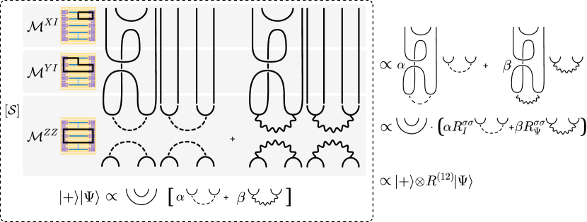
Figure 9: Mapping the measurement sequence for $[{\mathcal{S}}]$ to the braid of MZMs $1$ and $2$ on the computational qubit. The solid lines correspond to MZMs labeled 1, 2, 4, 3 from left to right, dashed lines correspond to MZMs fusing to the trivial state $I$, squiggly lines correspond to MZMs fusing to the fermionic state $\psi$. Left panel. The state $|+\rangle|\Psi\rangle$ is the two-qubit state prepared after applying ${\mathcal{M}^{XI}}$ to a generic state. The expression within the dashed-line box maps each measurement to its corresponding diagrammatic expression, with shaded sections separating different measurements. The sequence is read from bottom to top. Right panel. Applying the operator to the state on the left and collapsing the diagram results in the diagrammatic expressions shown, which can be rewritten as the braid on MZMs $1$ and $2$ applied to the state $|+\rangle|\Psi\rangle$. The diagrammatic calculus is explained in greater detail in Refs. 177 and 178 Appendix E.

Example measurement sequences to implement the braiding transformations associated with Pauli equivalence classes of single-qubit Clifford gates are given in Eq. 12-Eq. 16. Tracking the measurement outcomes allows us to write the explicit Pauli corrections associated with the sequences. Writing in terms of the ideal measurement projectors, we have

$${{\Pi}^{XI}_{s_{3}}}{{\Pi}^{YI}_{s_{2}}}{{\Pi}^{ZY}_{s_{1}}}{{\Pi}^{XI}_{s_{0}}} =\mathcal{O}^{s_{0}}_{s_{3}}\otimes Y^{\frac{1+s_{0}s_{1}s_{2}}{2}}XH,$$ (36)

$${{\Pi}^{XI}_{s_{3}}}{{\Pi}^{YI}_{s_{2}}}{{\Pi}^{ZZ}_{s_{1}}}{{\Pi}^{XI}_{s_{0}}} =\mathcal{O}^{s_{0}}_{s_{3}}\otimes Z^{\frac{1+s_{0}s_{1}s_{2}}{2}}S$$ (37)

$${{\Pi}^{XI}_{s_{3}}}{{\Pi}^{ZY}_{s_{2}}}{{\Pi}^{ZZ}_{s_{1}}}{{\Pi}^{XI}_{s_{0}}} =\mathcal{O}^{s_{0}}_{s_{3}}\otimes Y^{\frac{1-s_{0}s_{3}}{2}}X^{\frac{1+s_{1}s_{2}}{2}}HSH$$ (38)

$${{\Pi}^{XI}_{s_{4}}}{{\Pi}^{YI}_{s_{3}}}{{\Pi}^{ZY}_{s_{2}}}{{\Pi}^{ZZ}_{s_{1}}}{{\Pi}^{XI}_{s_{0}}} =\mathcal{O}^{s_{0}}_{s_{4}}\otimes Y^{\frac{1-s_{0}s_{2}s_{3}}{2}}Z^{\frac{1-s_{1}s_{2}}{2}}SH$$ (39)

$${{\Pi}^{XI}_{s_{4}}}{{\Pi}^{YI}_{s_{3}}}{{\Pi}^{ZZ}_{s_{2}}}{{\Pi}^{ZY}_{s_{1}}}{{\Pi}^{XI}_{s_{0}}} =\mathcal{O}^{s_{0}}_{s_{4}}\otimes X^{\frac{1+s_{1}s_{2}}{2}}Z^{\frac{1+s_{0}s_{1}s_{3}}{2}}HS,$$ (40)

where we have written the operator on the auxiliary qubit $\mathcal{O}^{s_{0}}_{s_{3}}$ as a shorthand for $|X_{s_{3}}\rangle\langle X_{s_{0}}|$. The equality in these expressions are up to overall constants.

The connection between the measurement sequence and the braiding transformation applied to the computational qubit can be explicitly seen through diagrammatic calculus, as shown for $[{\mathcal{S}}]$ in Fig. 9. Recall that for a pair of MZMs in state $|\Psi\rangle=\alpha|\sigma,\sigma;I\rangle+\beta|\sigma,\sigma;\psi\rangle$, a braiding transformation $R^{\sigma\sigma}$ acts on the state as

$$R^{\sigma\sigma}|\Psi\rangle =\alpha R^{\sigma\sigma}_{I}|\sigma,\sigma;I\rangle+\beta R^{\sigma\sigma}_{\psi}|\sigma,\sigma;\psi\rangle,$$ (41)

where $\{I,\psi,\sigma\}$ refer to the topological charges with non-Abelian fusion rules

$$\psi\times\psi =I$$ (42)

$$\psi\times\sigma =\sigma$$ (43)

$$\sigma\times\sigma =I+\psi.$$ (44)

The measurement sequence above is closely related to “one-bit teleportation” [179], a construction often used in the implementation of fault-tolerant gadgets (including the teleportation of non-Clifford gates using magic states as a resource) — the main difference being that, instead of an entangling unitary gate, a two-body measurement is performed to entangle the two qubits. The implementation of unitary operations in this manner has been previously described as “state transfer” [121], and is also the basis for measurement-based implementations of CNOT operations via lattice surgery [163]. The expression in Eq. 13 is also very similar to the measurement calculus formalism [180] used to describe the one-way model of quantum computation [181], although the qubit measurements in our Majorana platform are non-destructive (unlike typical measurements in optics-based platforms). These connections are elucidated by the concept of anyonic teleportation [23].

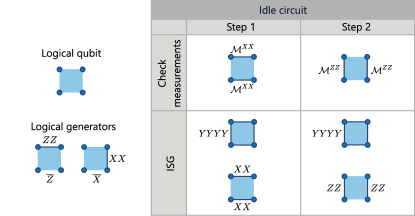
Figure 10: Top left. Four qubits (dots) form a logical qubit in the $2\times 2$ ladder code. Bottom left. The logical generators for the ladder code are $ZZ$ between horizontally adjacent qubits and $XX$ between vertically adjacent qubits. Right panel. The table shows the check measurements and instantaneous stabilizer group (ISG) for each step of the idle ladder code.

Appendix D Additional aspects of quantum error detection in the eight-qubit device

D.1 Ladder code summary

The idle circuit for the ladder code on a $2\times 2$ array of qubits is shown in Fig. 10. The instantaneous stabilizer group after a given step of the circuit corresponds to two-qubit Paulis of the measurements performed in that step, in addition to $YYYY$ on all four qubits (whose eigenvalue is inferred from multiplying the measurement outcomes for the previous two steps of the circuit). Errors are detected when the stabilizer eigenvalues change. The logical group generators are $\overline{Z}=ZZ$ between horizontal nearest neighbor qubits and $\overline{X}=XX$ between vertical nearest neighbor qubits.

A $\overline{ZZ}$ measurement in the ladder code corresponds to measuring the product of the $\overline{Z}$ on two adjacent logical qubits. The circuit shown in Fig. 11 achieves this: after steps 4 (and 1 when repeated) the product of $ZZZZ$ on the four middle qubits can be inferred from the measurement outcomes of the previous two steps. (Each qubit’s $YYYY$ stabilizer can be inferred after steps 2 and 3.)

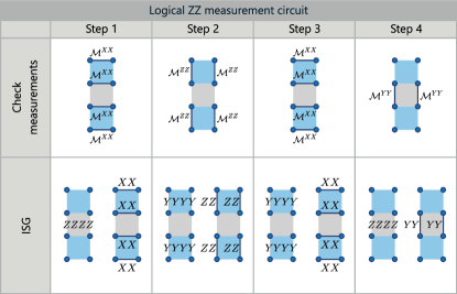
Figure 11: Check measurements and instantaneous stabilizer group for each step of the $\overline{ZZ}$ measurement circuit. The logical qubits are indicated by the blue shading, grey regions indicate qubits used to perform lattice surgery (the $\overline{ZZ}$ measurement).

D.2 Repetition code decay experiment

To compare the (post-selected) error rate of the logical $\overline{ZZ}$ measurement with the physical ${ZZ}$ measurement, we compare the repetition code run directly on a pair of physical qubits with the repetition code concatenated with the $2\times 2$ ladder code (Fig. 12). The repetition code consists of repeatedly measuring $ZZ$ and discarding any runs where the eigenvalue changes. As such, the stabilizer is $ZZ$, and the logical group is generated by $\widetilde{X}=XX$ and $\widetilde{Z}=ZI$. For the concatenated code, these correspond to $\widetilde{\overline{X}}=\overline{XX}=XXXX$ along a column of physical qubits, and $\widetilde{\overline{Z}}=\overline{ZI}=ZZ$ along a row of physical qubits. While $\widetilde{\overline{Z}}$ has weight on one more physical qubit than $\widetilde{Z}$, $\widetilde{\overline{X}}$ has weight on two more physical qubits than $\widetilde{X}$; as such we would expect the latter to manifest logical improvement for a larger region of parameter space than the former.

A logical state of the repetition code can be written as $|\psi_{i}\rangle=\alpha|00\rangle+\beta|11\rangle$, where $|0\rangle$ and $|1\rangle$ correspond to $Z$-eigenstates of the repetition code qubits. When the system is initialized in the state $|\psi_{i}\rangle=\frac{1}{\sqrt{2}}\left(|00\rangle+|11\rangle\right)$, a $\widetilde{Z}$ error can be detected by the expectation value of $XX$:

$$|\psi_{f}\rangle =ZI|\psi_{i}\rangle$$ (45)

$$\langle\psi_{f}|ZZ|\psi_{f}\rangle =1$$ (46)

$$\langle\psi_{f}|ZI|\psi_{f}\rangle =0$$ (47)

$$\langle\psi_{f}|XX|\psi_{f}\rangle =-1.$$ (48)

In experiment, the state can be prepared by measuring each qubit in $X$, post-selecting on the outcomes, and then running the (physical or logical) $ZZ$ measurement circuit.

When the system is initialized in the state $|\psi_{i}\rangle=|00\rangle$, a $\widetilde{X}$ error can be detected by the expectation value of $ZI$:

$$|\psi_{f}\rangle =XX|\psi_{i}\rangle$$ (49)

$$\langle\psi_{f}|ZZ|\psi_{f}\rangle =1$$ (50)

$$\langle\psi_{f}|ZI|\psi_{f}\rangle =-1$$ (51)

$$\langle\psi_{f}|XX|\psi_{f}\rangle =0.$$ (52)

The state can be prepared experimentally by measuring each qubit in $Z$, post-selecting on the outcomes, and then running the (physical or logical) $ZZ$ measurement.

To find the average logical improvement, defined in Eq. 19, we compare the repetition code run directly on the physical qubits to the repetition code run on the logical qubits for both sets of initial conditions.

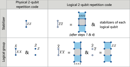
Figure 12: The stabilizers and logical group generators for the repetition code on both the physical and logical qubits.

D.3 Simulation details

To estimate the logical improvement, we perform an exact simulation of the decay experiment described within the effective noise model described in Sec.Sec. B parameterized by $p_{a},p_{1},p_{2}$. Starting with a prescribed initial state $\rho_{0}=|\psi_{i}\rangle\langle\psi_{i}|$, we run full density matrix simulations tracking the measurement outcomes through the corresponding noisy quantum instrument circuit [182, 183]. We thus obtain density matrix “trajectories” $\rho[\{s_{i}\}]$, which correspond to the (unnormalized) density matrices for a given set of measurement outcomes $\{s_{i}=\pm 1\}$. In principle, the number of such trajectories doubles with every measurement, leading to an exponential simulation cost in the length of the protocol; however, we can discard the trajectories corresponding to outcome combinations for which an error is detected. Here, we use a decoder constructed from the “checks” or “detectors” of the corresponding outcome code [184]. In addition, we can trace over those outcomes which are not needed in future checks. These optimizations keep the number of retained density matrices at a bounded, manageable number. Finally, the pertinent expectation values, as spelled out in the previous section, are computed using the system density matrix ignoring the outcomes, i.e., $\rho=\sum_{\{s_{i}=\pm 1\}}\rho[\{s_{i}\}]$, and the post-selected acceptance rate for the protocol is given merely by $\operatorname{tr}(\rho)$.

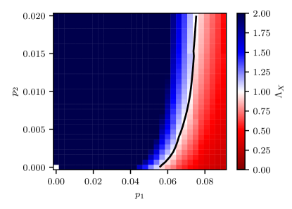
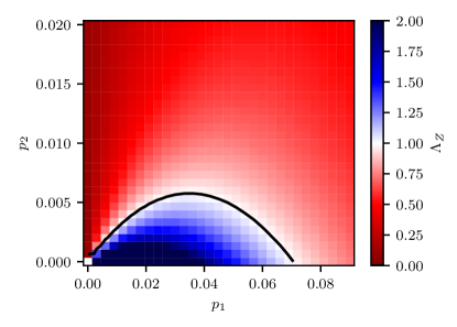
Figure 13: Ratio of physical to logical decay rates for $\widetilde{X}$ (top panel) and $\widetilde{Z}$ (bottom panel) for $p_{a}=0.01$, as defined in Eq. 53. The black curve bounds the region of logical improvement (blue). The region of logical improvement for $\widetilde{X}$ is much larger than that of $\widetilde{Z}$, as is expected from the weight of the corresponding physical operators.

In Fig. 13 we plot the ratio of the physical to logical decay rates associated with $\widetilde{X}$ and $\widetilde{Z}$, defined by

$$\Lambda_{X} =\frac{\lambda_{XX}}{\lambda_{\overline{XX}}}, \Lambda_{Z} =\frac{\lambda_{ZI}}{\lambda_{\overline{ZI}}}.$$ (53)

As discussed above, the former has a larger region of logical improvement than the latter due to the respective weights of the operators: $\overline{XX}=XXXX$ acts on two additional physical qubits compared to $XX$, while $\overline{ZI}=ZZ$ acts on one additional physical qubit compared to $ZI$.

References

- Nielsen and Chuang [2000] M. A. Nielsen and I. L. Chuang, Quantum Computation and Quantum Information (Cambridge University Press, Cambridge, 2000).
- Preskill [2022] J. Preskill, Lecture Notes for Ph219/CS219: Quantum Information (2022).
- Karzig et al. [2017a] T. Karzig, C. Knapp, R. M. Lutchyn, P. Bonderson, M. B. Hastings, C. Nayak, J. Alicea, K. Flensberg, S. Plugge, Y. Oreg, C. M. Marcus, and M. H. Freedman, Scalable designs for quasiparticle-poisoning-protected topological quantum computation with Majorana zero modes, Phys. Rev. B 95, 235305 (2017a).
- Plugge et al. [2017] S. Plugge, A. Rasmussen, R. Egger, and K. Flensberg, Majorana box qubits, New J. Phys. 19, 012001 (2017).
- Fidkowski et al. [2011] L. Fidkowski, R. M. Lutchyn, C. Nayak, and M. P. A. Fisher, Majorana zero modes in one-dimensional quantum wires without long-ranged superconducting order, Phys. Rev. B 84, 195436 (2011), arXiv:1106.2598 .
- Plugge et al. [2016] S. Plugge, L. A. Landau, E. Sela, A. Altland, K. Flensberg, and R. Egger, Roadmap to Majorana surface codes, Phys. Rev. B 94, 174514 (2016).
- Vijay et al. [2015] S. Vijay, T. H. Hsieh, and L. Fu, Majorana fermion surface code for universal quantum computation, Phys. Rev. X 5, 041038 (2015), arXiv:1504.01724 .
- Schrade and Fu [2018] C. Schrade and L. Fu, Majorana superconducting qubit, Physical Review Letters 121, 10.1103/physrevlett.121.267002 (2018).
- Kitaev [2001] A. Y. Kitaev, Unpaired Majorana fermions in quantum wires, Phys.-Usp. 44, 31 (2001), arXiv:cond-mat/0010440 .
- Lutchyn et al. [2010] R. M. Lutchyn, J. D. Sau, and S. Das Sarma, Majorana Fermions and a topological phase transition in semiconductor-superconductor heterostructures, Phys. Rev. Lett. 105, 077001 (2010), arXiv:1002.4033 .
- Oreg et al. [2010] Y. Oreg, G. Refael, and F. von Oppen, Helical liquids and Majorana bound states in quantum wires, Phys. Rev. Lett. 105, 177002 (2010), arXiv:1003.1145 .
- Aghaee et al. [2024] M. Aghaee et al., Interferometric Single-Shot Parity Measurement in an InAs-Al Hybrid Device (2024), arXiv:2401.09549 .
- Note [1] Ref. \rev@citealpAghaee24 was concerned with linear tetrons, in which the two topological wires are colinear.
- Kitaev [2003] A. Y. Kitaev, Fault-tolerant quantum computation by anyons, Ann. Phys. 303, 2 (2003), quant-ph/9707021 .
- Nayak et al. [2008] C. Nayak, S. H. Simon, A. Stern, M. Freedman, and S. Das Sarma, Non-Abelian anyons and topological quantum computation, Rev. Mod. Phys. 80, 1083 (2008), arXiv:0707.1889 .
- Cheng et al. [2009] M. Cheng, R. M. Lutchyn, V. Galitski, and S. Das Sarma, Splitting of majorana-fermion modes due to intervortex tunneling in a superconductor, Phys. Rev. Lett. 103, 107001 (2009).
- Knapp et al. [2018] C. Knapp, T. Karzig, R. M. Lutchyn, and C. Nayak, Dephasing of Majorana-based qubits, Phys. Rev. B 97, 125404 (2018).
- Mishmash et al. [2020] R. V. Mishmash, B. Bauer, F. von Oppen, and J. Alicea, Dephasing and leakage dynamics of noisy majorana-based qubits: Topological versus andreev, Physical Review B 101, 075404 (2020).
- Litinski and von Oppen [2018] D. Litinski and F. von Oppen, Quantum computing with majorana fermion codes, Phys. Rev. B 97, 205404 (2018).
- Hastings and Haah [2021] M. B. Hastings and J. Haah, Dynamically generated logical qubits, Quantum 5, 564 (2021).
- Gidney [2023] C. Gidney, A Pair Measurement Surface Code on Pentagons, Quantum 7, 1156 (2023).
- Grans-Samuelsson et al. [2023] L. Grans-Samuelsson, R. V. Mishmash, D. Aasen, C. Knapp, B. Bauer, B. Lackey, M. P. da Silva, and P. Bonderson, Improved pairwise measurement-based surface code (2023), arXiv:2310.12981 .
- Bonderson et al. [2008] P. Bonderson, M. Freedman, and C. Nayak, Measurement-only topological quantum computation, Phys. Rev. Lett. 101, 010501 (2008), arXiv:0802.0279 .
- Knapp et al. [2020] C. Knapp, J. I. Väyrynen, and R. M. Lutchyn, Number-conserving analysis of measurement-based braiding with majorana zero modes, Physical Review B 101, 10.1103/physrevb.101.125108 (2020).
- Alicea et al. [2011] J. Alicea, Y. Oreg, G. Refael, F. von Oppen, and M. P. A. Fisher, Non-Abelian statistics and topological quantum information processing in 1d wire networks, Nat. Phys. 7, 412 (2011), arXiv:1006.4395 .
- Sau et al. [2011] J. D. Sau, D. J. Clarke, and S. Tewari, Controlling non-Abelian statistics of Majorana fermions in semiconductor nanowires, Phys. Rev. B 84, 094505 (2011), arXiv:1012.0561 .
- van Heck et al. [2012] B. van Heck, A. R. Akhmerov, F. Hassler, M. Burrello, and C. W. J. Beenakker, Coulomb-assisted braiding of Majorana fermions in a Josephson junction array, New J. Phys. 14, 035019 (2012), arXiv:1111.6001 .
- Hyart et al. [2013] T. Hyart, B. van Heck, I. C. Fulga, M. Burrello, A. R. Akhmerov, and C. W. J. Beenakker, Flux-controlled quantum computation with Majorana fermions, Phys. Rev. B 88, 035121 (2013), arXiv:1303.4379 .
- Aasen et al. [2016] D. Aasen, M. Hell, R. V. Mishmash, A. Higginbotham, J. Danon, M. Leijnse, T. S. Jespersen, J. A. Folk, C. M. Marcus, K. Flensberg, and J. Alicea, Milestones toward Majorana-based quantum computing, Phys. Rev. X 6, 031016 (2016), arXiv:1511.05153 .
- Paetznick et al. [2023] A. Paetznick, C. Knapp, N. Delfosse, B. Bauer, J. Haah, M. B. Hastings, and M. P. da Silva, Performance of planar Floquet codes with Majorana-based qubits, PRX Quantum 4, 010310 (2023).
- Note [2] The measurement axes are labelled by the corresponding Pauli operators. Thus, even a two qubit measurement will still yield only two possible outcomes, corresponding to the different eigenvalues of the corresponding Pauli operator. Equivalently, we sometimes refer to these measurement as measuring only the parity of the operators, since outcomes on individual qubits are not revealed, only the product of the corresponding single qubit eigenvalues of each tensor factor.
- Note [3] Nevertheless, more conventional coherent oscillation experiments can be performed in these devices, and have been proposed as a means to characterize system properties such as the residual Majorana splitting and corresponding noise, see e.g. Refs. [18, 78].
- Gerlach and Stern [1922] W. Gerlach and O. Stern, Der experimentelle Nachweis der Richtungsquantelung im Magnetfeld, Z. Physik 9, 349 (1922).
- Note [4] The idea of verifying the existence of a qubit through two anticommuting measurements has been introduced before—Chao et al. [185] define a qubit in this way, and discuss the relation to more conventional notions of a qubit. Similarly, stronger guarantees about the action of the measurements can be obtained through self-testing protocols [186], although this is beyond the scope of this roadmap.
- Huie et al. [2023] W. Huie, L. Li, N. Chen, X. Hu, Z. Jia, W. K. C. Sun, and J. P. Covey, Repetitive readout and real-time control of nuclear spin qubits in atoms, PRX Quantum 4, 030337 (2023).
- Note [5] Note that the same protocols could be applied to logical qubits.
- Note [6] We emphasize the distinction between the usual definition of assignment error, which is the probability that a measurement classifier will assign an outcome to the observed measurement response that is different from the (inaccessible) true measurement outcome. Unlike the usual definition, the operational assignment error is directly measurable, but also accounts for state transitions during the measurement, not simply the classification errors.
- Note [7] Eqs. 2 and 4 can be obtained by noting .
- Schwinger [1960] J. Schwinger, Unitary operator bases, Proceedings of the National Academy of Sciences 46, 570 (1960), https://www.pnas.org/doi/pdf/10.1073/pnas.46.4.570 .
- Wootters and Fields [1989] W. K. Wootters and B. D. Fields, Optimal state-determination by mutually unbiased measurements, Annals of Physics 191, 363 (1989).
- Barenco et al. [1995] A. Barenco, C. H. Bennett, R. Cleve, D. P. DiVincenzo, N. Margolus, P. Shor, T. Sleator, J. A. Smolin, and H. Weinfurter, Elementary gates for quantum computation, Phys. Rev. A 52, 3457 (1995).
- Knill [2004] E. Knill, Fault-tolerant postselected quantum computation: Schemes (2004), arXiv:quant-ph/0402171 .
- Bravyi and Kitaev [2005] S. Bravyi and A. Kitaev, Universal quantum computation with ideal Clifford gates and noisy ancillas, Phys. Rev. A 71, 022316 (2005), arXiv:quant-ph/0403025 .
- Nichele et al. [2017] F. Nichele, A. C. C. Drachmann, A. M. Whiticar, E. C. T. O’Farrell, H. J. Suominen, A. Fornieri, T. Wang, G. C. Gardner, C. Thomas, A. T. Hatke, P. Krogstrup, M. J. Manfra, K. Flensberg, and C. M. Marcus, Scaling of Majorana zero-bias conductance peaks, Phys. Rev. Lett. 119, 136803 (2017).
- Suominen et al. [2017] H. J. Suominen, M. Kjaergaard, A. R. Hamilton, J. Shabani, C. J. Palmstrøm, C. M. Marcus, and F. Nichele, Zero-energy modes from coalescing Andreev states in a two-dimensional semiconductor-superconductor hybrid platform, Phys. Rev. Lett. 119, 176805 (2017).
- Aghaee et al. [2023] M. Aghaee et al. (Microsoft Quantum), InAs-Al hybrid devices passing the topological gap protocol, Phys. Rev. B 107, 245423 (2023).
- [47] J. D. Sau, B. I. Halperin, K. Flensberg, and S. Das Sarma, A number conserving theory for topologically protected degeneracy in one-dimensional fermions, arXiv:1106.4014 .
- Antipov et al. [2018] A. E. Antipov, A. Bargerbos, G. W. Winkler, B. Bauer, E. Rossi, and R. M. Lutchyn, Effects of gate-induced electric fields on semiconductor Majorana nanowires, Phys. Rev. X 8, 031041 (2018).
- Winkler et al. [2019] G. W. Winkler, A. E. Antipov, B. van Heck, A. A. Soluyanov, L. I. Glazman, M. Wimmer, and R. M. Lutchyn, Unified numerical approach to topological semiconductor-superconductor heterostructures, Phys. Rev. B 99, 245408 (2019).
- Motrunich et al. [2001] O. Motrunich, K. Damle, and D. A. Huse, Griffiths effects and quantum critical points in dirty superconductors without spin-rotation invariance: One-dimensional examples, Phys. Rev. B 63, 224204 (2001).
- Brouwer et al. [2011a] P. W. Brouwer, M. Duckheim, A. Romito, and F. von Oppen, Topological superconducting phases in disordered quantum wires with strong spin-orbit coupling, Phys. Rev. B 84, 144526 (2011a).
- Brouwer et al. [2011b] P. W. Brouwer, M. Duckheim, A. Romito, and F. von Oppen, Probability distribution of Majorana end-state energies in disordered wires, Phys. Rev. Lett. 107, 196804 (2011b).
- Akhmerov et al. [2011] A. R. Akhmerov, J. P. Dahlhaus, F. Hassler, M. Wimmer, and C. W. J. Beenakker, Quantized conductance at the Majorana phase transition in a disordered superconducting wire, Phys. Rev. Lett. 106, 057001 (2011).
- Stanescu et al. [2011] T. D. Stanescu, R. M. Lutchyn, and S. Das Sarma, Majorana fermions in semiconductor nanowires, Phys. Rev. B 84, 144522 (2011), arXiv:1106.3078 .
- Kells et al. [2012] G. Kells, D. Meidan, and P. W. Brouwer, Near-zero-energy end states in topologically trivial spin-orbit coupled superconducting nanowires with a smooth confinement, Phys. Rev. B 86, 100503 (2012).
- Prada et al. [2012] E. Prada, P. San-Jose, and R. Aguado, Transport spectroscopy of nanowire junctions with Majorana fermions, Phys. Rev. B 86, 180503 (2012), arXiv:1203.4488 .
- DeGottardi et al. [2013] W. DeGottardi, D. Sen, and S. Vishveshwara, Majorana fermions in superconducting 1D systems having periodic, quasiperiodic, and disordered potentials, Phys. Rev. Lett. 110, 146404 (2013).
- Adagideli et al. [2014] I. Adagideli, M. Wimmer, and A. Teker, Effects of electron scattering on the topological properties of nanowires: Majorana fermions from disorder and superlattices, Phys. Rev. B 89, 144506 (2014).
- Reeg et al. [2018] C. Reeg, O. Dmytruk, D. Chevallier, D. Loss, and J. Klinovaja, Zero-energy Andreev bound states from quantum dots in proximitized Rashba nanowires, Phys. Rev. B 98, 245407 (2018).
- Vuik et al. [2019] A. Vuik, B. Nijholt, A. R. Akhmerov, and M. Wimmer, Reproducing topological properties with quasi-Majorana states, SciPost Phys. 7, 061 (2019).
- Woods et al. [2021] B. D. Woods, S. Das Sarma, and T. D. Stanescu, Charge-impurity effects in hybrid Majorana nanowires, Phys. Rev. Appl. 16, 054053 (2021).
- Pan and Das Sarma [2020] H. Pan and S. Das Sarma, Physical mechanisms for zero-bias conductance peaks in majorana nanowires, Phys. Rev. Res. 2, 013377 (2020).
- Das Sarma and Pan [2021] S. Das Sarma and H. Pan, Disorder-induced zero-bias peaks in majorana nanowires, Phys. Rev. B 103, 195158 (2021).
- Das Sarma and Pan [2023] S. Das Sarma and H. Pan, Density of states, transport, and topology in disordered majorana nanowires, Phys. Rev. B 108, 085415 (2023).
- Das Sarma et al. [2023] S. Das Sarma, J. D. Sau, and T. D. Stanescu, Spectral properties, topological patches, and effective phase diagrams of finite disordered majorana nanowires, Phys. Rev. B 108, 085416 (2023).
- Pan and Das Sarma [2024] H. Pan and S. Das Sarma, Disordered majorana nanowires: Studying disorder without any disorder, Physical Review B 110, 10.1103/physrevb.110.075401 (2024).
- Antipov et al. [2025] A. Antipov, B. Bauer, S. Boutin, W. Cole, J. Gukelberger, F. Karimi, R. M. Lutchyn, and G. Winkler, Correlated disorder in one-dimensional topological superconductors (2025), in preparation.
- Akhmerov et al. [2009] A. R. Akhmerov, J. Nilsson, and C. W. J. Beenakker, Electrically detected interferometry of Majorana fermions in a topological insulator, Phys. Rev. Lett. 102, 216404 (2009), arXiv:0903.2196 .
- Fu and Kane [2009a] L. Fu and C. L. Kane, Probing neutral Majorana fermion edge modes with charge transport, Phys. Rev. Lett. 102, 216403 (2009a).
- Fu [2010] L. Fu, Electron teleportation via Majorana bound states in a mesoscopic superconductor, Phys. Rev. Lett. 104, 056402 (2010), arXiv:0909.5172 .
- Burnell et al. [2013] F. J. Burnell, A. Shnirman, and Y. Oreg, Measuring fermion parity correlations and relaxation rates in one-dimensional topological superconducting wires, Physical Review B 88, 10.1103/physrevb.88.224507 (2013).
- Houzet et al. [2013] M. Houzet, J. S. Meyer, D. M. Badiane, and L. I. Glazman, Dynamics of Majorana states in a topological Josephson junction, Phys. Rev. Lett. 111, 046401 (2013).
- Cheng and Lutchyn [2015] M. Cheng and R. Lutchyn, Fractional Josephson effect in number-conserving systems, Phys. Rev. B 92, 134516 (2015).
- Vijay and Fu [2016] S. Vijay and L. Fu, Physical implementation of a Majorana fermion surface code for fault-tolerant quantum computation, Phys. Scr. T168, 014002 (2016), arXiv:1509.08134 .
- Vijay and Fu [2016] S. Vijay and L. Fu, Teleportation-based quantum information processing with Majorana zero modes, Phys. Rev. B 94, 235446 (2016), arXiv:1609.00950 .
- Thamm and Rosenow [2021] M. Thamm and B. Rosenow, Transmission amplitude through a coulomb blockaded majorana wire, Phys. Rev. Res. 3, 023221 (2021).
- Drechsler et al. [2024] N. Drechsler, O. Lesser, and Y. Oreg, Electron interference as a probe of majorana zero modes, Phys. Rev. B 110, 134503 (2024).
- Sau and Das Sarma [2024] J. D. Sau and S. Das Sarma, Capacitance-based Fermion parity read-out and predicted Rabi oscillations in a Majorana nanowire, arXiv e-prints , arXiv:2406.18080 (2024), arXiv:2406.18080 [cond-mat.mes-hall] .
- Nadj-Perge et al. [2013] S. Nadj-Perge, I. K. Drozdov, B. A. Bernevig, and A. Yazdani, Proposal for realizing Majorana fermions in chains of magnetic atoms on a superconductor, Phys. Rev. B 88, 020407 (2013).
- Klinovaja et al. [2013] J. Klinovaja, P. Stano, A. Yazdani, and D. Loss, Topological superconductivity and Majorana fermions in RKKY systems, Phys. Rev. Lett. 111, 186805 (2013).
- Braunecker and Simon [2013] B. Braunecker and P. Simon, Interplay between classical magnetic moments and superconductivity in quantum one-dimensional conductors: Toward a self-sustained topological Majorana phase, Phys. Rev. Lett. 111, 147202 (2013).
- Pientka et al. [2013] F. Pientka, L. I. Glazman, and F. von Oppen, Topological superconducting phase in helical shiba chains, Phys. Rev. B 88, 155420 (2013).
- Nadj-Perge et al. [2014] S. Nadj-Perge, I. K. Drozdov, J. Li, H. Chen, S. Jeon, J. Seo, A. H. MacDonald, B. A. Bernevig, and A. Yazdani, Observation of Majorana fermions in ferromagnetic atomic chains on a superconductor, Science 346, 602 (2014), arXiv:1410.0682 .
- Zhang et al. [2016] J. Zhang, Y. Kim, E. Rossi, and R. M. Lutchyn, Topological superconductivity in a multichannel yu-shiba-rusinov chain, Phys. Rev. B 93, 024507 (2016).
- Cook and Franz [2011] A. Cook and M. Franz, Majorana fermions in a topological-insulator nanowire proximity-coupled to an -wave superconductor, Phys. Rev. B 84, 201105 (2011).
- Hosur et al. [2011] P. Hosur, P. Ghaemi, R. S. K. Mong, and A. Vishwanath, Majorana modes at the ends of superconductor vortices in doped topological insulators, Phys. Rev. Lett. 107, 097001 (2011).
- Vaitiekenas et al. [2020] S. Vaitiekenas, G. W. Winkler, B. van Heck, T. Karzig, M.-T. Deng, K. Flensberg, L. I. Glazman, C. Nayak, P. Krogstrup, R. M. Lutchyn, and C. M. Marcus, Flux-induced topological superconductivity in full-shell nanowires, Science 367, eaav3392 (2020).
- Wang et al. [2018] D. Wang, L. Kong, P. Fan, H. Chen, S. Zhu, W. Liu, L. Cao, Y. Sun, S. Du, J. Schneeloch, R. Zhong, G. Gu, L. Fu, H. Ding, and H.-J. Gao, Evidence for Majorana bound states in an iron-based superconductor, Science 362, 333 (2018).
- Kong et al. [2019] L. Kong, S. Zhu, M. Papaj, H. Chen, L. Cao, H. Isobe, Y. Xing, W. Liu, D. Wang, P. Fan, Y. Sun, S. Du, J. Schneeloch, R. Zhong, G. Gu, L. Fu, H.-J. Gao, and H. Ding, Half-integer level shift of vortex bound states in an iron-based superconductor, Nat. Phys. 15, 1181 (2019).
- Read and Green [2000] N. Read and D. Green, Paired states of fermions in two dimensions with breaking of parity and time-reversal symmetries and the fractional quantum Hall effect, Phys. Rev. B 61, 10267 (2000).
- Fu and Kane [2008] L. Fu and C. L. Kane, Superconducting proximity effect and Majorana fermions at the surface of a topological insulator, Phys. Rev. Lett. 100, 096407 (2008), arXiv:0707.1692 .
- Fu and Kane [2009b] L. Fu and C. L. Kane, Josephson current and noise at a superconductor/quantum-spin-Hall-insulator/superconductor junction, Phys. Rev. B 79, 161408(R) (2009b).
- Hasan and Kane [2010] M. Z. Hasan and C. L. Kane, Colloquium: Topological insulators, Rev. Mod. Phys. 82, 3045 (2010).
- Sau et al. [2010] J. D. Sau, R. M. Lutchyn, S. Tewari, and S. Das Sarma, Generic new platform for topological quantum computation using semiconductor heterostructures, Phys. Rev. Lett. 104, 040502 (2010), arXiv:0907.2239 .
- Alicea [2010] J. Alicea, Majorana fermions in a tunable semiconductor device, Phys. Rev. B 81, 125318 (2010).
- Sau et al. [2010] J. D. Sau, S. Tewari, R. M. Lutchyn, T. D. Stanescu, and S. Das Sarma, Non-Abelian quantum order in spin-orbit-coupled semiconductors: Search for topological Majorana particles in solid-state systems, Phys. Rev. B 82, 214509 (2010), arXiv:1006.2829 .
- Chung et al. [2011] S. B. Chung, H.-J. Zhang, X.-L. Qi, and S.-C. Zhang, Topological superconducting phase and Majorana fermions in half-metal/superconductor heterostructures, Phys. Rev. B 84, 060510 (2011).
- Duckheim and Brouwer [2011] M. Duckheim and P. W. Brouwer, Andreev reflection from noncentrosymmetric superconductors and Majorana bound-state generation in half-metallic ferromagnets, Phys. Rev. B 83, 054513 (2011).
- Potter and Lee [2012] A. C. Potter and P. A. Lee, Topological superconductivity and Majorana fermions in metallic surface states, Phys. Rev. B 85, 094516 (2012).
- Lutchyn et al. [2018] R. M. Lutchyn, E. P. A. M. Bakkers, L. P. Kouwenhoven, P. Krogstrup, C. M. Marcus, and Y. Oreg, Majorana zero modes in superconductor-semiconductor heterostructures, Nat. Rev. Mater. 3, 52 (2018).
- Laubscher et al. [2024] K. Laubscher, J. D. Sau, and S. Das Sarma, Majorana zero modes in gate-defined germanium hole nanowires, Phys. Rev. B 109, 035433 (2024).
- Sato et al. [2009] M. Sato, Y. Takahashi, and S. Fujimoto, Non-Abelian topological order in -wave superfluids of ultracold fermionic atoms, Phys. Rev. Lett. 103, 020401 (2009), arXiv:0901.4693 .
- Zhang et al. [2008] C. Zhang, S. Tewari, R. M. Lutchyn, and S. Das Sarma, superfluid from -wave interactions of fermionic cold atoms, Phys. Rev. Lett. 101, 160401 (2008).
- Willett et al. [1987] R. Willett, J. P. Eisenstein, H. L. Störmer, D. C. Tsui, A. C. Gossard, and J. H. English, Observation of an even-denominator quantum number in the fractional quantum Hall effect, Phys. Rev. Lett. 59, 1776 (1987).
- Pan et al. [1999] W. Pan, J.-S. Xia, V. Shvarts, D. E. Adams, H. L. Stormer, D. C. Tsui, L. N. Pfieffer, K. W. Baldwin, and K. W. West, Exact quantization of the even-denominator fractional quantum Hall state at Landau level filling factor, Phys. Rev. Lett. 83, 3530 (1999), arXiv:cond-mat/9907356 .
- Kumar et al. [2010] A. Kumar, G. A. Csáthy, M. J. Manfra, L. N. Pfeiffer, and K. W. West, Nonconventional odd-denominator fractional quantum Hall states in the second Landau level, Phys. Rev. Lett. 105, 246808 (2010).
- Zibrov et al. [2017] A. A. Zibrov, C. Kometter, H. Zhou, E. M. Spanton, T. Taniguchi, K. Watanabe, M. P. Zaletel, and A. F. Young, Tunable interacting composite fermion phases in a half-filled bilayer-graphene Landau level, Nature 549, 360 (2017).
- de C. Chamon et al. [1997] C. de C. Chamon, D. E. Freed, S. A. Kivelson, S. L. Sondhi, and X. G. Wen, Two point-contact interferometer for quantum Hall systems, Phys. Rev. B 55, 2331 (1997).
- Fradkin et al. [1998] E. Fradkin, C. Nayak, A. Tsvelik, and F. Wilczek, A Chern-Simons effective field theory for the Pfaffian quantum Hall state, Nucl. Phys. B 516, 704 (1998), arXiv:cond-mat/9711087 .
- Bonderson et al. [2006] P. Bonderson, A. Kitaev, and K. Shtengel, Detecting non-Abelian statistics in the fractional quantum Hall state, Phys. Rev. Lett. 96, 016803 (2006), arXiv:cond-mat/0508616 .
- Stern and Halperin [2006] A. Stern and B. I. Halperin, Proposed experiments to probe the non-Abelian quantum Hall state, Phys. Rev. Lett. 96, 016802 (2006), arXiv:cond-mat/0508447 .
- Willett et al. [2010] R. L. Willett, L. N. Pfeiffer, and K. W. West, Alternation and interchange of e/4 and e/2 period interference oscillations consistent with filling factor 5/2 non-Abelian quasiparticles, Phys. Rev. B 82, 205301 (2010), arXiv:0911.0345 .
- Nakamura et al. [2020] J. Nakamura, S. Liang, G. C. Gardner, and M. J. Manfra, Direct observation of anyonic braiding statistics, Nat. Phys. 16, 931 (2020).
- Note [8] When the overall island parity can change, the Pauli operators depend on the overall MZM parity.
- Karzig et al. [2017b] T. Karzig, C. Knapp, R. M. Lutchyn, P. Bonderson, M. B. Hastings, C. Nayak, J. Alicea, K. Flensberg, S. Plugge, Y. Oreg, et al., Scalable designs for quasiparticle-poisoning-protected topological quantum computation with majorana zero modes, Physical Review B 95, 235305 (2017b).
- Note [9] Eq. 8 assumes that measurement corresponds to distinguishing two Gaussians of equal width for an SNR definition of the distance between Gaussians divided by .
- Note [10] Additionally, non-equilibrium quasiparticles may contribute to the same error process with different scaling than thermally excited quasiparticles, however for the expected qubit volumes these are estimated to be subleading. This is in contrast to Ref. \rev@citealpAghaee24, where a lifetime of was observed in a configuration where all but one segment of the qubit device are tuned into a trivial superconducting regime. As such a configuration does not support a qubit, many of the error processes discussed here do not apply, and non-equilibrium quasiparticles remain as the dominant source of parity flips.
- Note [11] In the MBQB demonstration, it is never necessary for qubits to idle. Idle qubits are additionally subject to coherent rotations along the axis of the residual MZM coupling; these rotations result in an error since the measurement-based approach cannot be formulated in a rotating frame.
- Note [12] In practice, the band gap of the semiconductor sets a limit .
- Nielsen [2003] M. A. Nielsen, Quantum computation by measurement and quantum memory, Physics Letters A 308, 96–100 (2003), arXiv:quant-ph/0108020 .
- Perdrix [2005] S. Perdrix, State transfer instead of teleportation in measurement-based quantum computation, International Journal of Quantum Information 03, 219–223 (2005).
- Note [13] It is worth noting that braiding statistics have been experimentally emulated in qubit systems [187, 188, 189, 190, 191]. However, these experiments differ from topologically protected braiding transformations as discussed in this paper in that the topological state is not prepared as the ground state of the system’s Hamiltonian, but through a quantum circuit without active error correction. Therefore, there is no topological protection (such as that endowed by the topological gap) of these operations.
- Tran et al. [2020] A. Tran, A. Bocharov, B. Bauer, and P. Bonderson, Optimizing clifford gate generation for measurement-only topological quantum computation with majorana zero modes, SciPost Physics 8, 091 (2020).
- Karzig et al. [2016] T. Karzig, Y. Oreg, G. Refael, and M. H. Freedman, Universal Geometric Path to a Robust Majorana Magic Gate, Phys. Rev. X 6, 031019 (2016), arXiv:1511.05161 .
- Karzig et al. [2019] T. Karzig, Y. Oreg, G. Refael, and M. H. Freedman, Robust majorana magic gates via measurements, Physical Review B 99, 10.1103/physrevb.99.144521 (2019).
- Note [14] Although these Pauli operations are commonly referred to as corrections, they are very different in nature from error corrections inferred by a decoder associated with an error correction code. In this context, they are simply operations that depend on previous non-deterministic measurement outcomes, like the corrections that arise in quantum teleportation.
- Knill [2005] E. Knill, Quantum computing with realistically noisy devices, Nature 434, 39–44 (2005).
- Nielsen et al. [2021] E. Nielsen, J. K. Gamble, K. Rudinger, T. Scholten, K. Young, and R. Blume-Kohout, Gate Set Tomography, Quantum 5, 557 (2021).
- Note [15] Similar to how partial gate-set tomography is performed for X and Z measurements, the sequences must be prefixed with a randomized state preparation sequence, which we elide here for brevity. See \IfAppendixSec.Sec. A for details.
- Note [16] Residual MZM coupling through the wire can also result in coherent rotations when the measurement basis commutes with the MZM coupling basis. For example, MZM overlap along the same wire results in a single-qubit rotation during a measurement, which does not affect that measurement outcome but can affect a subsequent non-commuting measurement.
- Shor [1996] P. W. Shor, Fault-tolerant quantum computation, in Proc. 37th Symp. on Foundations of Computer Science (FOCS) (1996) p. 96, arXiv:quant-ph/9605011 .
- Steane [1996] A. M. Steane, Simple quantum error-correcting codes, Phys. Rev. A 54, 4741 (1996).
- Aharonov and Ben-Or [1997] D. Aharonov and M. Ben-Or, Fault-tolerant quantum computation with constant error, in Proceedings of the Twenty-Ninth Annual ACM Symposium on Theory of Computing, STOC ’97 (Association for Computing Machinery, New York, NY, USA, 1997) p. 176–188.
- Knill et al. [1998] E. Knill, R. Laflamme, and W. H. Zurek, Resilient quantum computation, Science 279, 342 (1998).
- Kitaev [2003] A. Y. Kitaev, Fault-tolerant quantum computation by anyons, Annals of Physics 303, 2 (2003).
- Terhal and Burkard [2005] B. M. Terhal and G. Burkard, Fault-tolerant quantum computation for local non-markovian noise, Phys. Rev. A 71, 012336 (2005).
- Aliferis et al. [2006] P. Aliferis, D. Gottesman, and J. Preskill, Quantum accuracy threshold for concatenated distance-3 codes, Quant. Inf. Comput. 6, 97 (2006), arXiv:quant-ph/0504218 .
- Willsch et al. [2018] D. Willsch, M. Willsch, F. Jin, H. De Raedt, and K. Michielsen, Testing quantum fault tolerance on small systems, Physical Review A 98, 10.1103/physreva.98.052348 (2018), arXiv:1805.05227 [quant-ph] .
- Vuillot [2018] C. Vuillot, Is error detection helpful on IBM 5Q chips?, Quantum Information and Computation 18, 10.26421/qic18.11-12 (2018), arXiv:1705.08957 [quant-ph] .
- Linke et al. [2017] N. M. Linke, M. Gutierrez, K. A. Landsman, C. Figgatt, S. Debnath, K. R. Brown, and C. Monroe, Fault-tolerant quantum error detection, Science Advances 3, 1701074 (2017), arXiv:1611.06946 [quant-ph] .
- Cane et al. [2021] R. Cane, D. Chandra, S. X. Ng, and L. Hanzo, Experimental characterization of fault-tolerant circuits in small-scale quantum processors, IEEE Access 9, 162996 (2021), arXiv:2112.04076 [quant-ph] .
- Hong et al. [2024] Y. Hong, E. Durso-Sabina, D. Hayes, and A. Lucas, Entangling four logical qubits beyond break-even in a nonlocal code, Phys. Rev. Lett. 133, 180601 (2024), arXiv:2406.02666 [quant-ph] .
- Bluvstein et al. [2024] D. Bluvstein, S. J. Evered, A. A. Geim, S. H. Li, H. Zhou, T. Manovitz, S. Ebadi, M. Cain, M. Kalinowski, D. Hangleiter, J. P. B. Ataides, N. Maskara, I. Cong, X. Gao, P. S. Rodriguez, T. Karolyshyn, G. Semeghini, M. J. Gullans, M. Greiner, V. Vuletic, and M. D. Lukin, Logical quantum processor based on reconfigurable atom arrays, Nature 626, 58 (2024), arXiv:2312.03982 [quant-ph] .
- Self et al. [2024] C. N. Self, M. Benedetti, and D. Amaro, Protecting expressive circuits with a quantum error detection code, Nat. Phys. 20, 219 (2024), arXiv:2211.06703 [quant-ph] .
- Yamamoto et al. [2024] K. Yamamoto, S. Duffield, Y. Kikuchi, and D. M. Ramo, Demonstrating Bayesian quantum phase estimation with quantum error detection, Phys. Rev. Research 6, 013221 (2024), arXiv:2306.16608 [quant-ph] .
- Ryan-Anderson et al. [2021] C. Ryan-Anderson, J. G. Bohnet, K. Lee, D. Gresh, A. Hankin, J. P. Gaebler, D. Francois, A. Chernoguzov, D. Lucchetti, N. C. Brown, T. M. Gatterman, S. K. Halit, K. Gilmore, J. Gerber, B. Neyenhuis, D. Hayes, and R. P. Stutz, Realization of real-time fault-tolerant quantum error correction, Phys. Rev. X 11, 041058 (2021), arXiv:2107.07505 [quant-ph] .
- Postler et al. [2024] L. Postler, F. Butt, I. Pogorelov, C. D. Marciniak, S. Heußen, R. Blatt, P. Schindler, M. Rispler, M. Müller, and T. Monz, Demonstration of fault-tolerant Steane quantum error correction, PRX Quantum 5, 030326 (2024), arXiv:2312.09745 [quant-ph] .
- Paetznick et al. [2024] A. Paetznick, M. P. da Silva, C. Ryan-Anderson, et al., Demonstration of logical qubits and repeated error correction with better-than-physical error rates (2024), arXiv:2404.02280 [quant-ph] .
- Reichardt et al. [2024] B. W. Reichardt, D. Aasen, R. Chao, A. Chernoguzov, et al., Demonstration of quantum computation and error correction with a tesseract code (2024), arXiv:2409.04628 [quant-ph] .
- Harper and Flammia [2019] R. Harper and S. T. Flammia, Fault-tolerant logical gates in the IBM Quantum Experience, Phys. Rev. Lett. 122, 080504 (2019), arXiv:1806.02359 [quant-ph] .
- Krinner et al. [2022] S. Krinner, N. Lacroix, A. Remm, A. D. Paolo, E. Genois, C. Leroux, C. Hellings, S. Lazar, F. Swiadek, J. Herrmann, G. J. Norris, C. K. Andersen, M. Müller, A. Blais, C. Eichler, and A. Wallraff, Realizing repeated quantum error correction in a distance-three surface code, Nature 605, 669 (2022), arXiv:2112.03708 [quant-ph] .
- Google Quantum AI [2023] Google Quantum AI, Suppressing quantum errors by scaling a surface code logical qubit, Nature 614, 676 (2023), arXiv:2207.06431 [quant-ph] .
- Putterman et al. [2024] H. Putterman, K. Noh, C. T. Hann, G. S. MacCabe, S. Aghaeimeibodi, et al., Hardware-efficient quantum error correction using concatenated bosonic qubits (2024), arXiv:2409.13025 [quant-ph] .
- Ofek et al. [2016] N. Ofek, A. Petrenko, R. Heeres, P. Reinhold, Z. Leghtas, B. Vlastakis, Y. Liu, L. Frunzio, S. M. Girvin, L. Jiang, et al., Extending the lifetime of a quantum bit with error correction in superconducting circuits, Nature 536, 441 (2016).
- Sivak et al. [2023] V. Sivak, A. Eickbusch, B. Royer, S. Singh, I. Tsioutsios, S. Ganjam, A. Miano, B. Brock, A. Ding, L. Frunzio, et al., Real-time quantum error correction beyond break-even, Nature 616, 50 (2023).
- Ni et al. [2023] Z. Ni, S. Li, X. Deng, Y. Cai, L. Zhang, W. Wang, Z.-B. Yang, H. Yu, F. Yan, S. Liu, et al., Beating the break-even point with a discrete-variable-encoded logical qubit, Nature 616, 56 (2023).
- Google Quantum AI [2024a] Google Quantum AI, Quantum error correction below the surface code threshold, Nature 10.1038/s41586-024-08449-y (2024a).
- Google Quantum AI [2024b] Google Quantum AI, Demonstrating dynamic surface codes (2024b), arXiv:2412.14360 [quant-ph] .
- Lacroix et al. [2024] N. Lacroix, A. Bourassa, F. J. Heras, L. M. Zhang, J. Bausch, A. W. Senior, T. Edlich, N. Shutty, V. Sivak, A. Bengtsson, et al., Scaling and logic in the color code on a superconducting quantum processor (2024), arXiv:2412.14256 [quant-ph] .
- Haah and Hastings [2022] J. Haah and M. B. Hastings, Boundaries for the honeycomb code, Quantum 6, 693 (2022).
- Gidney et al. [2021] C. Gidney, M. Newman, A. Fowler, and M. Broughton, A fault-tolerant honeycomb memory, Quantum 5, 605 (2021).
- Gidney et al. [2022] C. Gidney, M. Newman, and M. McEwen, Benchmarking the planar honeycomb code, Quantum 6, 813 (2022).
- Horsman et al. [2012] D. Horsman, A. G. Fowler, S. Devitt, and R. Van Meter, Surface code quantum computing by lattice surgery, New Journal of Physics 14, 123011 (2012).
- Note [17] For the scheme described below, the ladder code can only correct errors.
- Bacon [2006] D. Bacon, Operator quantum error correcting subsystems for self-correcting quantum memories, Phys. Rev. A 73, 012340 (2006), arXiv:quant-ph/0506023 .
- Shor [1995] P. W. Shor, Scheme for reducing decoherence in quantum computer memory, Physical review A 52, R2493 (1995).
- Aasen et al. [2023] D. Aasen, J. Haah, P. Bonderson, Z. Wang, and M. Hastings, Fault-tolerant hastings-haah codes in the presence of dead qubits (2023), arXiv:2307.03715 [quant-ph] .
- Beverland et al. [2022] M. E. Beverland, P. Murali, M. Troyer, K. M. Svore, T. Hoefler, V. Kliuchnikov, G. H. Low, M. Soeken, A. Sundaram, and A. Vaschillo, Assessing requirements to scale to practical quantum advantage (2022), arXiv:2211.07629 [quant-ph] .
- Gidney and Ekerå [2021] C. Gidney and M. Ekerå, How to factor 2048 bit RSA integers in 8 hours using 20 million noisy qubits, Quantum 5, 433 (2021).
- Davies and Lewis [1970] E. B. Davies and J. T. Lewis, An operational approach to quantum probability, Communications in Mathematical Physics 17, 239 (1970).
- Wiseman and Milburn [2010] H. Wiseman and G. Milburn, Quantum Measurement and Control (Cambridge University Press, 2010).
- Note [18] We write instead of when the relevant quantum state is clear from context.
- de Bruijn [1946] N. G. de Bruijn, A combinatorial problem, Nederl. Akad. Wetensch., Proc. 49, 758 (1946).
- Boutin et al. [2025] S. Boutin, T. Karzig, T. El Dandachi, R. V. Mishmash, M. P. da Silva, J. Gukelberger, R. M. Lutchyn, and B. Bauer, Predictive simulations of the dynamical response of mesoscopic devices (2025), in preparation.
- Aasen et al. [2025] D. Aasen, B. Bauer, P. Bonderson, and C. Knapp, Electron poisoning of majorana-based qubits, In preparation (2025).
- Kern et al. [2005] O. Kern, G. Alber, and D. L. Shepelyansky, Quantum error correction of coherent errors by randomization, The European Physical Journal D 32, 153–156 (2005).
- Bonderson [2007] P. H. Bonderson, Non-Abelian anyons and interferometry, Ph.D. thesis, California Institute of Technology (2007).
- Kitaev [2006] A. Kitaev, Anyons in an exactly solved model and beyond, Ann. Phys. 321, 2 (2006), arXiv:cond-mat/0506438 .
- Zhou et al. [2000] X. Zhou, D. W. Leung, and I. L. Chuang, Methodology for quantum logic gate construction, Phys. Rev. A 62, 052316 (2000).
- Danos et al. [2007] V. Danos, E. Kashefi, and P. Panangaden, The measurement calculus, J. ACM 54, 8–es (2007).
- Raussendorf and Briegel [2001] R. Raussendorf and H. J. Briegel, A one-way quantum computer, Phys. Rev. Lett. 86, 5188 (2001).
- Bombín et al. [2023] H. Bombín, C. Dawson, R. V. Mishmash, N. Nickerson, F. Pastawski, and S. Roberts, Logical blocks for fault-tolerant topological quantum computation, PRX Quantum 4, 020303 (2023).
- Kliuchnikov et al. [2023] V. Kliuchnikov, M. Beverland, and A. Paetznick, Stabilizer circuit verification (2023), arXiv:2309.08676 [quant-ph] .
- Delfosse and Paetznick [2023] N. Delfosse and A. Paetznick, Spacetime codes of clifford circuits (2023), arXiv:2304.05943 [quant-ph] .
- Chao et al. [2017] R. Chao, B. W. Reichardt, C. Sutherland, and T. Vidick, Overlapping qubits (2017), arXiv:1701.01062 [quant-ph] .
- Irfan et al. [2020] A. A. M. Irfan, K. Mayer, G. Ortiz, and E. Knill, Certified quantum measurement of majorana fermions, Phys. Rev. A 101, 032106 (2020).
- Song et al. [2018] C. Song, D. Xu, P. Zhang, J. Wang, Q. Guo, W. Liu, K. Xu, H. Deng, K. Huang, D. Zheng, et al., Demonstration of topological robustness of anyonic braiding statistics with a superconducting quantum circuit, Physical Review Letters 121, 030502 (2018).
- Satzinger et al. [2021] K. Satzinger, Y.-J. Liu, A. Smith, C. Knapp, M. Newman, C. Jones, Z. Chen, C. Quintana, X. Mi, A. Dunsworth, et al., Realizing topologically ordered states on a quantum processor, Science 374, 1237 (2021).
- Stenger et al. [2021] J. P. Stenger, N. T. Bronn, D. J. Egger, and D. Pekker, Simulating the dynamics of braiding of majorana zero modes using an ibm quantum computer, Physical Review Research 3, 033171 (2021).
- Google Quantum AI and Collaborators [2023] Google Quantum AI and Collaborators, Non-Abelian braiding of graph vertices in a superconducting processor, Nature 618, 264 (2023).
- Xu et al. [2024] S. Xu, Z.-Z. Sun, K. Wang, H. Li, Z. Zhu, H. Dong, J. Deng, X. Zhang, J. Chen, Y. Wu, et al., Non-abelian braiding of fibonacci anyons with a superconducting processor, Nature Physics 20, 1469 (2024).