When More is Less: Understanding Chain-of-Thought Length in LLMs

Abstract

Chain-of-thought (CoT) reasoning enhances the multi-step reasoning capabilities of large language models (LLMs) by breaking complex tasks into smaller, manageable sub-tasks. Researchers have been exploring ways to guide models to generate more complex CoT processes to improve the reasoning ability of LLMs, such as long CoT and the test-time scaling law. However, for most models and tasks, does an increase in CoT length consistently lead to improved reasoning accuracy? In this paper, we observe a nuanced relationship: as the number of reasoning steps increases, performance initially improves but eventually decreases. To understand this phenomenon, we provide a piece of evidence that longer reasoning processes are increasingly susceptible to noise. We theoretically prove the existence of an optimal CoT length and derive a scaling law for this optimal length based on model capability and task difficulty. Inspired by our theory, we conduct experiments on both synthetic and real world datasets and propose Length-filtered Vote to alleviate the effects of excessively long or short CoTs. Our findings highlight the critical need to calibrate CoT length to align with model capabilities and task demands, offering a principled framework for optimizing multi-step reasoning in LLMs.

1 Introduction

Large language models (LLMs) have demonstrated impressive capabilities in solving complex reasoning tasks (Brown et al., 2020; Touvron et al., 2023). One approach to enhance their performance on such tasks is Chain of Thought (CoT) reasoning (Wei et al., 2022), where the model generates explicit intermediate reasoning steps before arriving at the final answer. The CoT process can be seen as a divide-and-conquer strategy (Zhang et al., 2024), where the model breaks a complex problem into simpler sub-problems, solves each one individually, and then combines the results to reach a final conclusion. It is commonly believed that longer CoT generally improves the performance, especially on more difficult tasks (Fu et al., 2023; Jin et al., 2024). On the other hand, a concise CoT (Nayab et al., 2024) has been shown to incur a decreased performance penalty on math problems. But does performance consistently improve as the length of the CoT increases?

In this paper, we conduct comprehensive and rigorous experiments on synthetic arithmetic datasets and find that for CoT length, longer is not always better (Figure 1). Specifically, by controlling task difficulty, we observe that as the reasoning path lengthens, the model’s performance initially improves but eventually deteriorates, indicating the existence of an optimal length. This phenomenon can be understood by modeling the CoT process as a task decomposition and subtask-solving structure. While early-stage decomposition helps break down the problem, excessively long reasoning paths lead to error accumulation—where a single mistake can mislead the entire chain of thought.

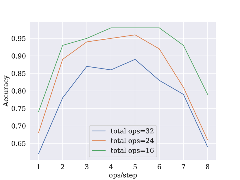
(a) Small model with 6 layers

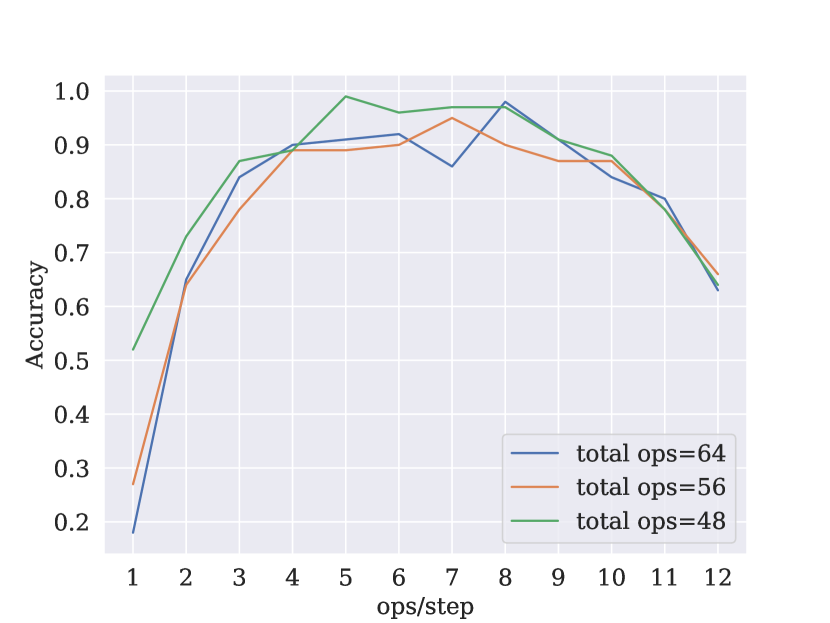
(b) Large model with 9 layers

Figure 1: Evaluation of the relationship between CoT length and final performance on synthetic arithmetic datasets. The models used are different layers of GPT-2, with all other hyperparameters unchanged. The results show that accuracy initially increases and then decreases as the number of operations per step grows (while the total number of steps decreases), indicating that both overthinking and underthinking can harm LLM reasoning abilities.

Our experimental results also show that the optimal CoT length is directly influenced by both model capability and task complexity. Intuitively, for more challenging tasks, a deeper decomposition is required. Meanwhile, a more capable model can handle moderately complex subtasks in a single step, reducing the need for excessive reasoning steps. Furthermore, as task difficulty increases, the optimal length of each reasoning step tends to grow to prevent the total number of steps from becoming excessively long.

Then in Section 4, we provide a formal and rigorous theoretical explanation for these findings. Under a simplified setting, we show that each of the above conclusions can be described mathematically. We also present a more general version of our theory that applies to a broader range of conditions.

Following the theoretical analyses of optimal CoT length, we further validate these insights by examining their effects on real-world LLM behavior at test-time and their influence on CoT training. In Section 5.1, we conduct experiments on real-world math problems using various sizes of open-source LLMs. The results further confirm that a longer CoT is not always better, but should adapt to model size and task difficulty. Furthermore, in Section 5.2, we train models using data with the optimal CoT length rather than randomly selected lengths. The results are striking: a small model trained on optimal-length CoT can even outperform larger models trained on randomly chosen CoT lengths. This highlights the significant impact of CoT length in training data on model performance.

Inspired by both theoretical and experimental findings, we propose methods to leverage the optimal CoT length during inference. Specifically, we enhance the standard majority voting approach by introducing Length-filtered Vote. This adaptive method selects answers with the optimal CoT length while filtering out those that are either too short or too long.

2 Related Work

Chain of Thought Large Language Models (LLMs) (Brown et al., 2020) have demonstrated remarkable abilities in complex reasoning tasks by breaking down challenging problems into intermediate steps before arriving at the final answer (Wei et al., 2022). Numerous researchers have proposed various approaches to enhance the CoT reasoning capabilities of LLMs. Least-to-most prompting (Zhou et al., 2023) decomposes a complex problem into a series of simpler sub-problems, solving them sequentially, where the solution to each subproblem builds upon the answers to previously solved sub-problems. Tree of thoughts (Yao et al., 2023) enables LLMs to engage in deliberate decision-making by exploring multiple reasoning paths, self-evaluating options, and dynamically adjusting the reasoning process through backtracking or look-ahead strategies to make globally optimal choices. Similarly, Divide-and-Conquer methods (Zhang et al., 2024; Meng et al., 2024) divide the input sequence into multiple sub-inputs, which can significantly improve LLM performance in specific tasks. Despite their differences, these methods share a common characteristic: they all treat the CoT process as a framework for decomposition and subtask-solving. Similarly, our study adopts this perspective.

CoT Understanding In addition to the methods mentioned above, many works aim to formalize the CoT process and explore why it is effective. Circuit complexity theory has been used to analyze the computational complexity of problems that transformers can solve with and without CoT, providing a theoretical understanding of CoT’s effectiveness (Feng et al., 2023; Li et al., 2024b). Cui et al. (2024) theoretically demonstrate that, compared to Stepwise ICL, integrating reasoning from earlier steps (Coherent CoT) enhances transformers’ error correction capabilities and prediction accuracy. Ton et al. (2024) quantify the information gain at each reasoning step in an information-theoretic perspective to understand the CoT process. Furthermore, Li et al. (2024a) show that fast thinking without CoT results in larger gradients and greater gradient differences across layers compared to slow thinking with detailed CoT, highlighting the improved learning stability provided by the latter. Ye et al. (2024) investigate CoT in a controlled setting by training GPT-2 models on a synthetic GSM dataset, revealing hidden mechanisms through which language models solve mathematical problems. Unlike these theoretical studies, our work focuses on the impact of different lengths of CoT on final performance and tries to understand CoT from task decomposition and error accumulation perspective.

Overthinking With the remarkable success of OpenAI’s o1 model, test-time computation scaling has become increasingly important. More and more works (Snell et al., 2024; Chen et al., 2024d; Wu et al., 2024; Brown et al., 2024) have explored the scaling laws during inference using various methods, such as greedy search, majority voting, best-of-n, and their combinations. They concluded that with a compute-optimal strategy, a smaller base model can achieve non-trivial success rates, and test-time compute can outperform larger models. This highlights the importance of designing optimal inference strategies.

However, Chen et al. (2024a) hold a contrastive opinion that in some cases, the performance of the Best-of-N method may decline as $N$ increases. Similarly, the overthinking phenomenon (Chen et al., 2024c) becomes more and more important as o1-like reasoning models allocate excessive computational resources to simple problems (e.g., $2+3=5$) with minimal gains. These findings indicate the need to balance computation based on model capabilities and task difficulty. In our study, we focus on different types of CoT reasoning, categorized by CoT length. Moreover, we theoretically identify a balanced CoT strategy that adapts to model size and task difficulty, optimizing performance under these constraints.

3 Influence of Chain-of-Thought Length on Arithmetic Tasks

Figure 2: Computation tree of arithmetic expression $5+(4+((2+1)+3))$.

To begin, we aim to empirically investigate the relationship between reasoning performance and CoT length. Therefore, we need to control a given model to generate reasoning chains of varying lengths for a specific task. Unfortunately, no existing real-world dataset or model fully meets these strict requirements. Real-world reasoning tasks, such as GSM8K or MATH (Cobbe et al., 2021; Hendrycks et al., 2021), do not provide multiple solution paths of different lengths, and manually constructing such variations is challenging. Moreover, it is difficult to enforce a real-world model to generate a diverse range of reasoning paths for a given question.

Given these limitations, we begin our study with experiments on synthetic datasets. Notably, even when working with real-world datasets, we observe behavioral patterns that align well with the findings derived from synthetic data (Section 5.1).

3.1 Problem Formulation

To investigate the effect of CoT length in a controlled manner, we design a synthetic dataset of simplified arithmetic tasks with varying numbers of reasoning steps in the CoT solutions. The necessity and rationale for simplified arithmetic tasks will be further discussed in the Appendix B.

Definition 3.1 (Problem).

In a simplified setting, an arithmetic task $q$ is defined as a binary tree of depth $T$. The root and all non-leaf nodes are labeled with the $+$ operator, while each leaf node contains a numerical value (mod 10). In addition, we impose a constraint that every non-leaf node must have at least one numerical leaf as a child.

The bidirectional conversion method between arithmetic expressions and computation trees is as follows: keeping the left-to-right order of numbers unchanged, the computation order of each "+" or tree node is represented by tree structure or bracket structures. For example, consider the task $5+(4+((2+1)+3))$ with $T=4$. The corresponding computation tree is defined as Figure 2.

To ensure that CoT solutions of the same length have equal difficulty for a specific problem, we assume that each reasoning step performs the same operations within a single CoT process. A more rigorous discussion will be conducted in Appendix B.2.

Definition 3.2 (Solution).

We define a $t$-hop CoT with a fixed each step length of $t$ as a process that executes $t$ operations starting from the deepest level and moving upward recursively.

According to this definition, the execution sequence is uniquely determined. For example, one way to solve expression in Figure 2 is by performing one addition at a time:

$$5+(4+((2+1)+3))=\texttt{<1>}$$ (1)

$$2+1=3$$ (2)

$$3+3=6$$

$$4+6=0$$

$$5+0=5\texttt{<END>.}$$

Another approach is to perform two additions at a time:

$$5+(4+((2+1)+3))=\texttt{<2>}$$ (3)

$$(2+1)+3=6$$

$$5+(4+6)=5\texttt{<END>.}$$

The latter approach is half as long as the former, but each reasoning step is more complex. This illustrates a clear trade-off between the difficulty of each subtask and the total number of reasoning steps.

In practice, when $t$ does not evenly divide $T$, the final step performs $T\mod t$ operations. To guide the model in generating the desired CoT length, we insert the control token <t> after the question and before the beginning of the solution. To preserve the parentheses that indicate the order of operations, we construct expressions in Polish notation. However, for readability, we present each problem in its conventional form throughout the article.

3.2 Experiment Setup

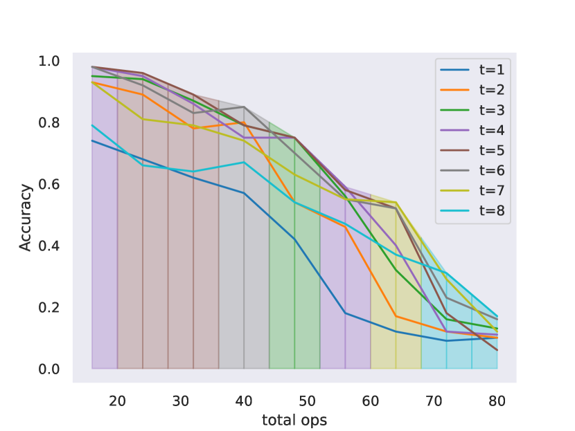
(a) Small model with 6 layers

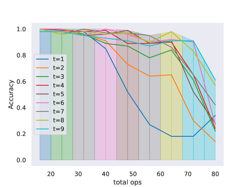
(b) Large model with 9 layers

Figure 3: The envelope curve shows how the performance of optimal operators in a single step ($t$) changes as the task becomes more difficult. The different colors of the envelope curve correspond to the best-performing operators in one step ($t$) for the given set of total operators.

Dataset The datasets used for training different models are identical and are constructed from tasks with varying total operators $T$ and solutions with different $t$.

Model Since model depth plays a critical role in mathematical reasoning (Ye et al., 2024), we trained GPT-2 models with varying numbers of layers, keeping all other parameters (e.g., heads, dimensions) constant, to assess the impact of model capacity. Our experimental results provide evidence that models with more layers are capable of performing more operations in a single step, without the need for CoT.

Train and Test For each problem, we train the model to start generating from the control token <t> to ensure that it can independently determine which CoT solution to use. During testing, we guide the model to produce the required $t$-hop CoT by inserting the control token <t> right before the question. More details can be found in Appendix D.

3.3 Experimental Results

U-curve For convenience, we present how the final accuracy changes as the number of operators performed per step $t$ increases, which corresponds to a decrease in the number of reasoning steps, for tasks of varying difficulty (total operators). Figures 1(a) and 1(b) show the performance of small and large models on easy tasks (16, 24, 32 operators) and hard tasks (48, 56, 64 operators) respectively.

The results (Figure 1) align well with our theory, demonstrating that as the number of reasoning steps increases, the final performance initially improves and then declines. Subsequent experiments will explore how the optimal CoT length changes with model capability and task difficulty.

Envelope Curve Figure 3(a) and 3(b) illustrate the envelope curve, where different colors represent the optimal single-step length. The results indicate that as the task becomes more challenging, CoT with a larger single-step reasoning length $t$ achieves the best performance. This can be interpreted as a mechanism to regulate the total number of CoT steps—shorter single-step lengths require more CoT steps to complete the task.

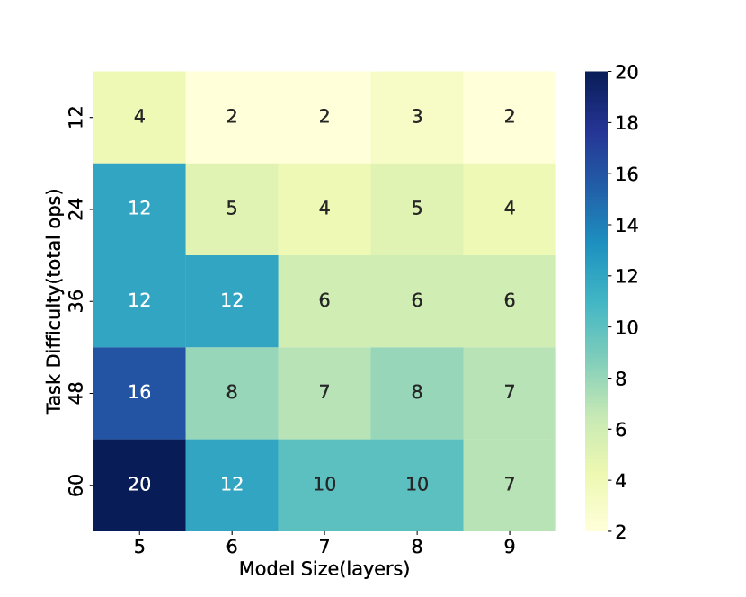
Figure 4: Heat map of optimal CoT length in different model sizes and task difficulties.

Optimal CoT length shifts To further investigate how the optimal CoT length changes with model capability and task difficulty, we trained models of varying sizes (ranging from 5 to 9 layers) on tasks of different difficulties (from 16 to 64 operators). For each combination of model size and task difficulty, we recorded the optimal number of reasoning steps.

Figure 4 illustrates two key findings. First, an increase in the number of reasoning steps is beneficial for solving more challenging problems, indicating that harder tasks require more steps to achieve optimal performance. Second, the optimal number of reasoning steps decreases as the model size increases, suggesting that stronger models can handle more complex reasoning within fewer steps.

4 Theoretical Analysis

In this section, we provide a theoretical analysis of the CoT process for the simplified arithmetic tasks defined above and explain the empirical results observed in synthetic datasets. All proofs of the paper are deferred to Appendix F.

4.1 Setup

Let $N\in\mathbb{N^{+}}$ represent the total number of steps in the CoT process. As defined earlier, $T$ denotes the total number of operators in the given question, and $t=\left\lceil\frac{T}{N}\right\rceil$ represents the number of operators processed in each reasoning step. We use $t_{i}$ to denote the subtask in the $i$-th reasoning step (e.g., $2+1$ in Eq. (2)), and $a_{i}$ to represent the corresponding answer (e.g., $3$ in Eq. (2)).

Definition 4.1.

Given task $q$ with total operators $T$ (Definition 3.1) and model $\theta$, to a specific $N$, we define an $N$ step ($t$-hop in Definition 3.2) CoT process as

$$P(a_{N}|q,\theta)=\prod^{N}_{i=1}P(t_{i}|H_{i-1},q,\theta)P(a_{i}|t_{i},H_{i-1},q,\theta),$$

where $H_{k}=[t_{1},a_{1},\cdots,t_{k},a_{k}]$ collects the first $k$ steps in the $N$-step CoT process, and $a_{N}$ is not only the answer of the final subtask $t_{i}$, but the answer to the whole task $q$ as well.

Let $a_{i}^{*}$ denote the correct answer to subtask $t_{i}$, and $t_{i}^{*}$ the correct next subtask given the history reasoning steps $H_{i-1}$, total task $q$, and total step number $N$. To estimate the final accuracy $A(N)=P(a_{N}=a_{N}^{*}|q,\theta)$, we need to separately estimate the sub-question accuracy $P(t_{i}=t_{i}^{*}|H_{i-1},q,\theta)$ and the sub-answer accuracy $P(a_{i}=a^{*}|t_{i},H_{i-1},q,\theta)$.

For the sub-question accuracy, as observed in our experiments, the loss for tokens appearing in $t_{i}$ remains almost constant across different values of $N$ and model sizes (see Appendix C). We assume that the noise affecting tokens in each subtask $t_{i}$, denoted as $\sigma(T)\in[0,1)$, is positively correlated with the total number of operators $T$. Intuitively, as the number of operators increases, extracting the correct subtask becomes more challenging.

For the sub-answer accuracy, it is clear that when given subtask $t_{i}$, $P(a_{i}=a^{*}|t_{i},H_{i-1},q,\theta)$ is independent of the history reasoning steps $H_{i-1}$ and is only influenced by the model $\theta$ and the difficulty of the subtask $t_{i}$. For each model, we define its capability $M$ based on the reasoning boundary (Chen et al., 2024b). Specifically, we consider $M$ as the maximum number of operators the model can compute in a single step without CoT.

$$M=M(\theta)=\max_{t}\left\{P(a_{i}=a^{*}|t_{i},\theta)>0,|t_{i}|=t\right\},$$ (4)

where $|t_{i}|$ refers to the number of operators in subtask $t_{i}$. In the following discussion, we focus only on CoT chains that do not exceed the model’s capability, which is $t<M.$ Hence, we define the error rate of each subtask answer as $E(N,M,T)\in[0,1)$. propositionfinalacc The total accuracy of $N$-step reasoning is

$$A(N)=\alpha\left((1-E(N,M,T))(1-\sigma(T))\right)^{N},$$ (5)

where $\alpha$ denotes a constant value independent of $N$.

Proposition 5 establishes a differentiable functional relationship between total accuracy and CoT length $N$. Once we obtain estimates for $E(N,M,T)$ and $\sigma(T)$, we can determine the optimal $N(M,T)$. For simplicity, in the following discussion, we allow $N$, $M$, and $T$ to be real numbers. In Section 4.2, we analyze the case of a linear error rate, while in Section 4.3, we explore more general error functions.

4.2 A Simple Case with Linear Error

An estimation of $\sigma(T)$. To simplify the setting, we assume $\sigma(T)=\frac{T}{C}$, where $C$ is a hyperparameter representing the maximum number of operators the model can handle, which is solely influenced by the training data. To ensure that the model is capable of generating a reasonable subtask (even if it is incorrect), we consider a finite range $T\in[0,0.9C]$, ensuring that the subtask accuracy rate $1-\sigma(T)$ remains within $[0.1,1]$.

An estimation of $E(N,M,T)$. We define the model answer’s error rate $E(N,M,T)=\frac{T}{N}/{M}$ as the ratio between the number of subtask operators and the model’s capacity $M$ (Eq. (4)) that the maximum number of operators the model can compute in a single step. Therefore, $1-\frac{T}{NM}>0$.

According to Proposition 5, a simplified total accuracy of $N$-step reasoning is

$$A(N)=\alpha\left(\left(1-\frac{T}{C}\right)\left(1-\frac{T}{NM}\right)\right)^{N}.$$ (6)

theoremOptimalN In a simplified setting, for a given model capability $M$ and task difficulty $T$, the final accuracy $A(N)$ (Eq. (6)) increases initially and then decreases as the number of reasoning steps $N$ increases. Besides, there exists an optimal

$$N(M,T)=\frac{TZ}{M(Z+1)}$$ (7)

that maximizes the final accuracy, where $Z=W_{-1}\left(-\frac{1-\frac{T}{C}}{e}\right)$, and $W_{-1}(x)$ denotes the smaller branch of the Lambert function, which satisfies the equation $we^{w}=x$.

Theorem 4.2 shows the optimal $N(M,T)$ is only affected by two factors $M$ and $T$. Through the expression of $N$, we can naturally derive the following three observations about the trend of $N$ with respect to changes in $M$ or $T$:

Corollary 4.2.

$\frac{T}{N(T,M)}=M\left(1+\frac{1}{Z}\right)$ increases monotonically with $T$, which aligns the envelope curve result well.

corollaryNwithT $N(M,T)$ increases monotonically with $T$, which shows that as the total task becomes more difficult, the optimal number of reasoning steps increases.

Corollary 4.3.

$N(M,T)$ decreases monotonically with $M$, which shows that as the capability of the model becomes stronger, it is easier for the model to solve one-step subtask reasoning, which leads to the decrease of the total task decomposition number.

4.3 Extension to General Error Functions

In the simple case above, we discussed the trend of overall accuracy with respect to $N$ and the variation of optimal $N$ with $M$ and $T$, assuming the subtask error rate is a linear function. In the following discussion, we aim to derive conclusions corresponding to more general error rate functions. We find that as long as the error function satisfies some basic assumptions, the above conclusions still hold. A detailed discussion of basic assumptions will be conducted in Appendix E.

theoremgeneral For any noise function $0<\sigma(T)<1$ and a subtask error rate function $0<E(N,M,T)<1$ satisfying Assumption E.1 and E.2, a general final accuracy function $A(N)$ (Proposition 5) has the following properties:

• $\lim_{N\rightarrow+\infty}A(N)\rightarrow 0$

• If $A(N)$ has the point of maximum value $N^{*}>1$, then $N^{*}$ has a lower bound

  $$N^{*}\geq N(M,T)=E^{-1}\left(1-\frac{1}{e^{2}(1-\sigma(T))}\right),$$ (8)

where $E^{-1}$ is the inverse function of $E(N,M,T)$ with respect to $N$, which has the same monotonicity as $E$ with respect to $M$ and $T$. Therefore, we have similar corollaries as in the linear case.

Corollary 4.4.

As the model becomes stronger, $E^{-1}$ decreases monotonically with respect to $M$, which leads to decrease of $N(M,T)$.

Corollary 4.5.

As the task becomes harder, $E^{-1}$ is monotonically increasing with respect to $T$, which leads to an increase of $N(M,T)$.

5 Empirical Examination of Optimal CoT Length

Following the theoretical analyses of optimal CoT length in Section 4, we further validate these insights on both real-world LLM behaviors at test time and its influence on CoT training.

5.1 Optimal CoT Length of LLMs on MATH

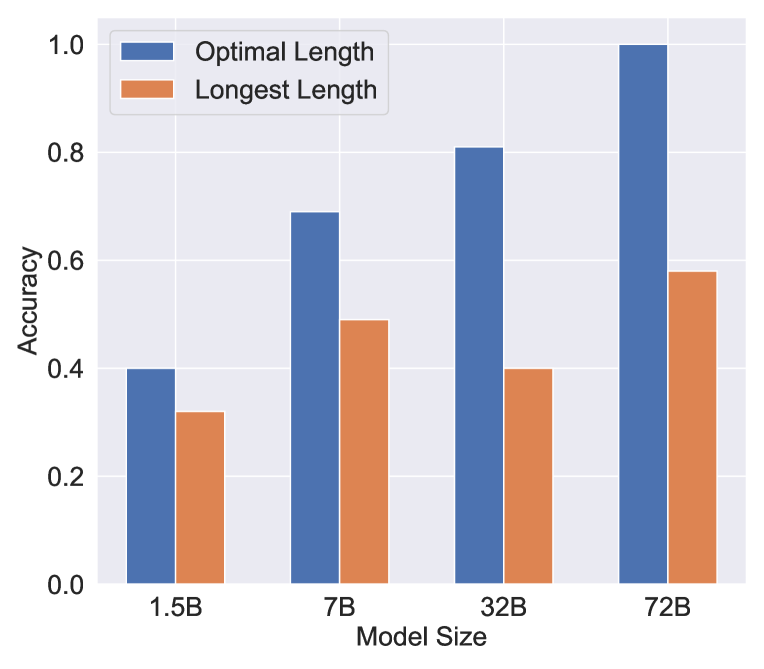
(a) Optimal length v.s. Longest length

(b) Optimal length v.s. Model size

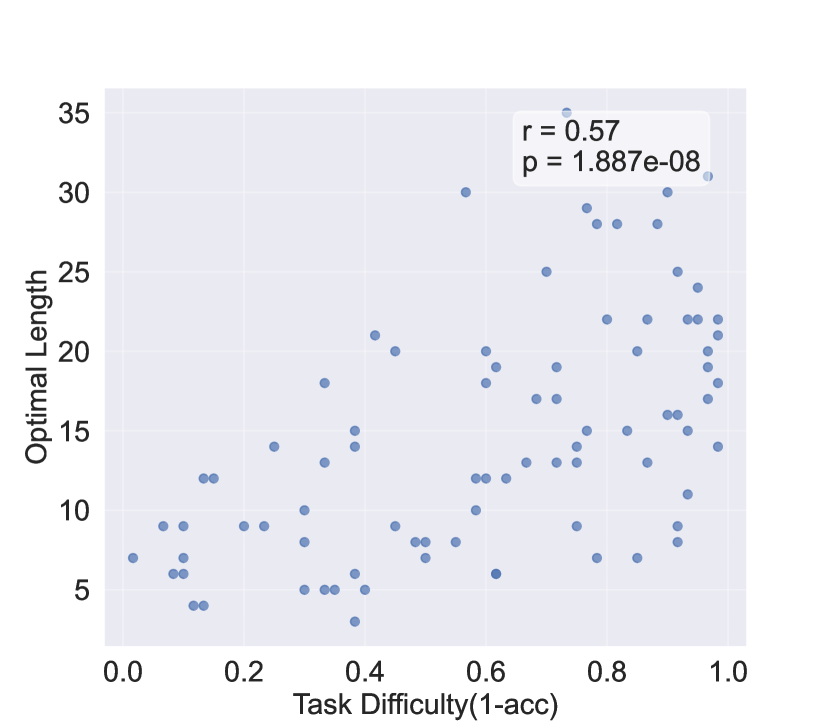
(c) Optimal length v.s. Task difficulty

Figure 5: Evaluation on MATH datasets with Qwen2.5 Series Instruct models.

To validate our theory on real-world tasks with LLMs, we consider the MATH (Hendrycks et al., 2021) algebra dataset (Level 5), which includes challenging competition-level mathematics problems requiring multi-step reasoning. We select Qwen2.5 series Instruct models (Qwen et al., 2025) to investigate behaviors among models with different capabilities. More details can be found in Appendix A.1.

Optimal Length and Model Capability In this section, we randomly select 30 questions from the dataset, generating 60 samples for each question, resulting in a total of 1,800 samples for each model. The results, shown in Figure 5(a), demonstrate that for each model, the longest number of steps is not the best one. Additionally, the optimal CoT length decreases as the model size increases, from 14 steps for the 1.5B model to 4 steps for the 72B model (Figure 5(b)). This trend aligns with our theory that larger models perform better with fewer reasoning steps, as they are more capable of effectively handling single-step reasoning.

Impact of Task Difficulty In this part, we evaluate how the optimal CoT length changes with task difficulty. To achieve this, we randomly select 100 questions from the dataset, generating 60 samples for each question to ensure the number of reasoning steps is calculated accurately. We assume that a question with lower accuracy among the 60 samples is more difficult for the model, using 1-accuracy as a proxy for the relative difficulty of each question(the larger the harder).

We then plot a scatter plot of accuracy versus optimal CoT length and calculate the correlation. As shown in Figure 5(c), a significant correlation ($p=1e-8<<0.05$) between task difficulty and optimal CoT length. Results on different models are shown in Appendix A.2. This finding supports our theory that harder tasks require more steps to solve effectively.

5.2 Implications for Training with CoT Data

In the previous synthetic dataset experiments (Section 3), we generated solutions with varying step lengths by training our model on data sampled with random CoT lengths. Now that we have identified the optimal CoT length, an important question arises:

Can we construct a dataset that contains only CoT solutions with optimal lengths, tailored to the current model size and task difficulty?

To explore this, we conduct experiments on a synthetic dataset. The baseline model is trained on CoT step lengths following a uniform distribution, while the optimal model is trained exclusively on the optimal CoT lengths identified in Figure 4.

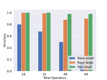
Figure 6: Comparison of training on CoTs with optimal lengths versus random lengths: Base refers to a model trained on data with random CoT lengths, while Opt refers to a model trained on data with optimal CoT lengths.

During testing, we allow the model to choose the CoT types on its own. The results shown in Figure 6 demonstrate that with a carefully designed training dataset, a smaller model can achieve significantly better performance—nearly 100% accuracy—even surpassing a larger model trained on base dataset.

However, in real-world datasets, the same problem may be associated with reasoning chains of varying lengths, none of which necessarily correspond to the optimal one. This experiment highlights the importance of carefully selecting CoT length when training models for chain-of-thought reasoning.

Algorithm 1 Length-filtered Vote

1:Input: Model $f_{\theta}$, Question $q$, Space of All Possible Answers $A$, Number of Total Groups $M$, Number of Selected Groups $K$, Group Width $D$

2:Output: Final Answer $\hat{a}$

3:Sample candidates $c_{1},\dots,c_{n}\stackrel{{\scriptstyle i.i.d.}}{{\sim}}f_{\theta}(q)$

4:Define $\mathcal{A}(c)$ as the corresponding answer of candidates $c$.

5:Define $p_{j}\in[0,1]^{|\mathcal{A}|}$ as the frequency of each answer in length group $L_{j}$.

6:for $j=1$ to $m$ do $L_{j}=\{c_{i}\mid\ell(c_{i})\in\left[D*(j-1),D*j\right),i=1,\cdots,n\}$

7:  for $a\in\mathcal{A}$ do

$$p_{j}[a]=\frac{\sum_{c\in L_{j}}\mathbb{I}(\mathcal{A}(c)=a)}{|L_{j}|}$$

8:  end for

9:end for

10:$\{s_{1},\dots,s_{K}\}=\arg\min_{S\subseteq\{1,\dots,M\},|S|=K}\sum_{s\in S}H(p_{s})$

11:$\hat{a}=\arg\max_{a\in A}\sum_{c\in L_{s_{1}}\cup\dots\cup L_{s_{K}}}\mathbb{I}(\mathcal{A}(c)=a)$

12:return $\hat{a}$

6 Length-filtered Vote

Section 5.2 highlights the importance of aligning the CoT length with the model’s capabilities and the task’s difficulty. However, achieving this alignment requires an accurate estimation of both the task and the model. Moreover, given a pretrained model, how can we leverage the optimal CoT length without any prior estimation of the task or even the model itself?

In this section, we propose a length-aware variant of majority vote, Length-filtered vote, where we use prediction uncertainty as a proxy to filter reliable CoT lengths. As in majority vote, given a model $f_{\theta}$, a question $q$, a ground truth answer $a^{*}$, we first sample a set of answer candidates independently $c_{1},\dots,c_{n}\stackrel{{\scriptstyle i.i.d.}}{{\sim}}f_{\theta}(q)$. After that, instead of direct vote, we group the answers based on their corresponding CoT length $\ell(c_{i})$ (discussed in Appendix A.1) into groups with equal bandwidth $D$ (by default, we set $D=2$), denoted as $\{L_{j}\}_{j=1}^{m}$. As our theory suggests that the prediction accuracy of CoT paths is peaked around a certain range of CoT length, we identify such groups through the prediction uncertainty of the answers within each group, based on the intuition that lower uncertainty implies better predictions. Specifically we calculate the Shannon entropy of the final answers given by the CoT chains in each group $L_{i}$, denoted as $H(L_{i})$. We then select $K$ (by default, we set $K=3$) out of $M$ groups that has the smallest entropy and then perform majority vote only on these selected groups. We summarize it in Algorithm 1.

Table 1: Performance of different models with varying sample numbers for Direct Vote on all candidates and Length-filtered Vote.

Model	Method	Number of Samples
		20	30	40	50
Llama3.1-8B-Ins	Direct Vote	35%	38%	39%	38%
	Length-filtered Vote	36%	42%	42%	41%
Qwen2.5-7B-Ins	Vote	34%	35%	36%	34%
	Length-filtered Vote	36%	40%	38%	40%

We evaluate the propose method against vanilla majority vote (i.e., self-consistency) (Wang et al., 2023) on a randomly chosen subset of 100 questions from the GPQA dataset, a more challenging collection of multiple-choice questions. The results in Table 1 show that our filtered vote consistently outperforming vanilla majority vote at different sample numbers and have little performance degradation as the sample number increases. This indicates the importance of considering the influence CoT length in the reasoning process.

7 Conclusion

In this paper, we conduct experiments on a simplified synthetic dataset, drawing clear conclusions on how the CoT length affects the final performance. Our study also provides valuable insights, showing that the optimal CoT length should adapt to both model size and task difficulty. Furthermore, we present a rigorous theoretical framework demonstrating the non-monotonic scaling behavior of CoT length and how it is influenced by model size and task difficulty. Additionally, we conduct experiments on real-world datasets, yielding similar results. We also propose methods that can benefit from the optimal CoT length during both training and test phases. In this way, our analysis offers concrete theoretical and empirical insights into developing LLMs that adaptively select the appropriate reasoning length, avoiding either overthinking or underthinking.

Appendix

.tocmtappendix mtchapternone mtappendixsubsection

Appendix A Additional Real world Experiment Details

A.1 Implementation Details

In real world experiments, we investigate how the optimal CoT length varies between these two models and with different question difficulties. To create solutions with varying step lengths, we follow [Fu et al., 2023] by using in-context examples (8-shots) with three different levels of complexity to guide the model in generating solutions with different step counts. For each set of in-context examples, we sample 20 times, resulting in a total of 60 samples per question.

When calculating the number of steps, we separate the full reasoning chain using "\n"[Fu et al., 2023] and remove empty lines caused by "\n\n". Then we consider the total number of lines as the CoT length. Since the MATH dataset questions are challenging, leading to high variability in final CoT lengths, we scale the CoT length using length = length // 5. As we are primarily observing trends, this scaling is considered acceptable.

When evaluating the results, questions with accuracy $<0.01$ or $>0.99$ (indicating all incorrect or all correct responses) are excluded, as their accuracy does not vary with step length changes.

A.2 Task Difficulty v.s. Optimal CoT Lengths

To further investigate the relationship between task difficulty and optimal CoT lengths on real world datasets, we conduct experiments on different models. The results (Figure 7 and 8) are impressive that results on all models show a significant correlation between the task difficulties and optimal lengths.

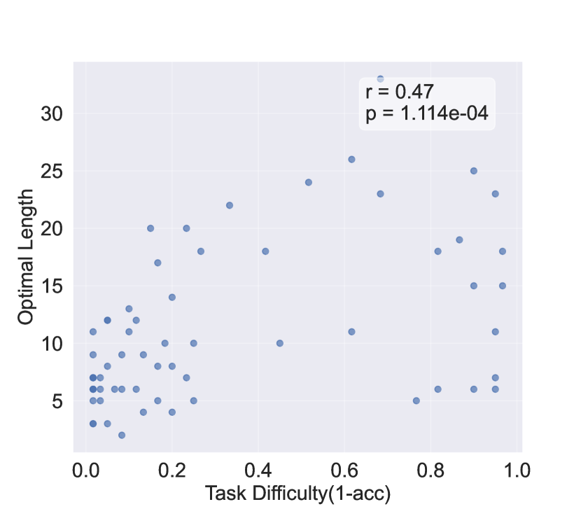
(a) Qwen2.5 7B Instruct

(b) Qwen2.5 14B Instruct

Figure 7: Evaluation between task difficulties and optimal CoT lengths on MATH datasets with Qwen2.5 Series Instruct models.

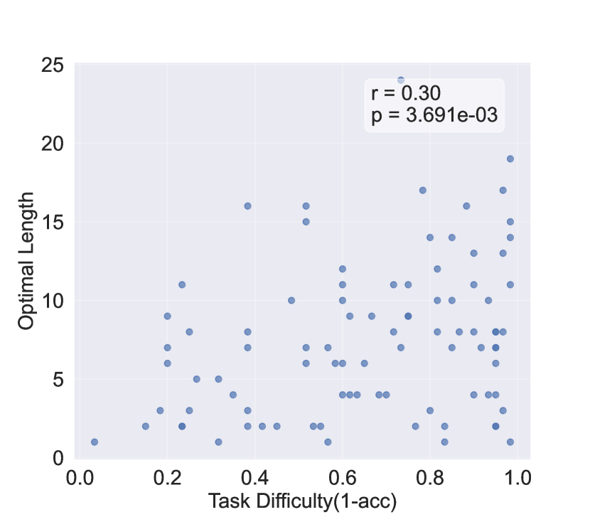
(a) Llama 3.1 8B Instruct

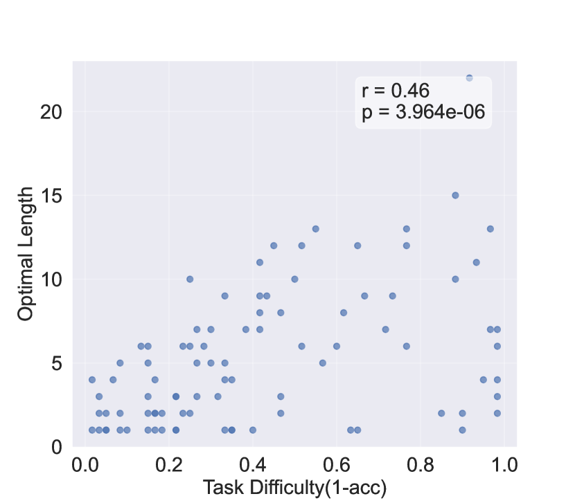
(b) Llama 3.1 70B Instruct

Figure 8: Evaluation between task difficulties and optimal CoT lengths on MATH datasets with LLama3.1 Series Instruct models.

Appendix B Synthetic Arithmetic Problem Discussions

B.1 Contrast to vanilla arithmetic problem

Why pruning? Initially, we intended to create a synthetic dataset for regular arithmetic tasks, but we quickly realized that the computation tree for such tasks is uncontrollable. For example, consider the task $1*2+3*4$. We hoped to compute $2$ operators in one step, but found it impossible because the addition needs to be computed after the two multiplications, and we cannot aggregate two multiplications in one subtask. Therefore, pruning the computation tree becomes essential.

Why only focusing on addition? There are two reasons why we focus on arithmetic tasks involving only addition: first, it simplifies pruning, as the order of operations can be controlled solely by parentheses; second, it facilitates the computation of sub-tasks, since parentheses do not affect the final result, and the model only needs to compute the sum of all the numbers when solving a sub-task. We aim for the model to handle longer sub-tasks, thereby allowing a broader study of the impact of CoT length.

Will the simplified synthetic dataset impact the diversity of the data? We need to clarify that even with pruning, the structure of the expressions will still vary because swapping the left and right child nodes of each non-leaf node in the computation tree results in different expressions. When $T>30$, the number of possible variations exceeds $1\times 10^{9}$.

B.2 Same Subtask Difficulty

A Chain-of-Thought (CoT) containing sub-tasks of varying difficulty can be seen as a mixture of CoTs with the same difficulty level. On the other hand, allowing CoTs to generate sub-tasks of different lengths increases the overall difficulty of CoTs of the same length, making them harder to study. Third, under Assumption E.1, convexity analysis shows that the final accuracy function (Proposition 5) is concave. Therefore, to maximize accuracy, all sub-tasks should have the same difficulty level.

Appendix C Subtask Loss

As we observed in training losses, the loss of subtask generation tokens (e.g. $1+2$) for the easiest subtask($t=1$) is about 3 times larger than the hardest subtask ($t=12$), while the loss ratio for subtask answer tokens is $1e4$. Therefore, it is acceptable for taking the subtask error rate constant with $t$.

Besides, there is no obvious pattern showing the model sizes affect the subtask loss. Moreover, the smallest model and the largest model have almost the same subtask loss. Therefore, in our settings, we take model size as irrelevant with the subtask error rate.

Appendix D Synthetic Experiment Details

In default, we train different models(layers ranging from 5 to 9) on the same dataset, which included mixed questions with total operators $T\in[12,80]$ and random sampled CoT solutions with each step operators $t\in[1,12]$. All other parameters are kept the same with the huggingface GPT-2 model. During the training process, the CoT indicator token <t> is also trained, so that during test-time, we can let the model decide which type of CoT it will use by only prompting the model with the question. For each model, we train $25000$ iterations with batch size that equals 256. During test-time, we test 100 questions for each $T$ and $t$. All experiments can be conducted on one NVIDIA A800 80G GPU.

Appendix E General Error Functions

Assumption E.1.

$E(N,M,T)$ satisfies the following reasonable conditions:

• $0<E(N=1,M,T)<1$

• $\lim_{N\rightarrow+\infty}E(N,M,T)=0$

• $E(N,M,T)$ is monotonically deceasing with $N$, since more detailed decomposition leads to easier subtask.

• $E(N,M,T)$ is convex with $N$, since the benefits of further decomposing an already fine-grained problem($N$ is large) are less than the benefits of decomposing a problem that has not yet been fully broken down($N$ is small).

• $E(N,M,T)$ is monotonically deceasing with $M$, since stronger models have less subtask error rate.

• $E(N,M,T)$ is monotonically increasing with $T$, since harder total task leads to harder subtask while $N,M$ are the same.

Assumption E.2.

$\sigma(T)$ is monotonically increasing with $T$

Appendix F Proof

In this section, we provide the proofs for all theorems.

F.1 Proof of Proposition 5

*

Proof.

In each subtask $t_{i}$, which contains $t$ operators, there are $2t+1$ tokens (as the number of numerical tokens is one more than the number of operators). Therefore, the accuracy of each subtask is given by

$$P(t_{i}=t_{i}^{*}|H_{i-1},q,\theta)=\left(1-\sigma(T)\right)^{2t+1}.$$ (9)

In our theoretical analysis, for simplicity, we allow $t$ to be a fraction, defined as $t=\frac{T}{N}$, and assume that each subtask has the same level of difficulty given $T$ and $N$. Under this assumption, we have the final accuracy:

$$A(N) =P(a_{N}=a_{N}^{*}|q,\theta)$$ (10)

$$=\prod^{N}_{i=1}P(t_{i}=t_{i}^{*}|H_{i-1},q,\theta)P(a_{i}=a_{i}^{*}|t_{i},H_{i-1},q,\theta)$$ (11)

$$=\prod^{N}_{i=1}\left(1-\sigma(T)\right)^{2t+1}\left(1-E(N,M,T)\right)$$ (12)

$$=\left(1-\sigma(T)\right)^{N(2t+1)}\left(1-E(N,M,T)\right)^{N}$$ (13)

$$=\left(1-\sigma(T)\right)^{2T}\left((1-E(N,M,T))(1-\sigma(T))\right)^{N}$$ (14)

$$=\alpha\left((1-E(N,M,T))(1-\sigma(T))\right)^{N}$$ (15)

∎

F.2 Proof of Theorem 4.2

*

Proof.

Given Eq. (6) that

$$A(N)=\alpha\left(\left(1-\frac{T}{C}\right)\left(1-\frac{T}{NM}\right)\right)^{N}$$ (16)

We consider function

$$f(x)\;=\;\Bigl{[}\bigl{(}1-\tfrac{T}{Mx}\bigr{)}\,\bigl{(}1-\tfrac{T}{C}\bigr{)}\Bigr{]}^{x}.$$ (17)

For convenience, define

$$g(x)\;=\;\ln\bigl{(}f(x)\bigr{)}\;=\;x\;\ln\!\Bigl{[}\bigl{(}1-\tfrac{T}{Mx}\bigr{)}\,\bigl{(}1-\tfrac{T}{C}\bigr{)}\Bigr{]}.$$

Thus,

$$g^{\prime}(x)=\Bigl{[}\ln\bigl{(}1-\tfrac{T}{Mx}\bigr{)}\;+\;\frac{T}{Mx\,\bigl{(}1-\tfrac{T}{Mx}\bigr{)}}\Bigr{]}\;+\;\ln\bigl{(}1-\tfrac{T}{C}\bigr{)}.$$

Set $g^{\prime}(x)=0$:

$$\ln\Bigl{[}\bigl{(}1-\tfrac{T}{Mx}\bigr{)}\,\bigl{(}1-\tfrac{T}{C}\bigr{)}\Bigr{]}\;+\;\frac{T}{Mx\bigl{(}1-\tfrac{T}{Mx}\bigr{)}}=0.$$

Let $A\;=\;\frac{1}{1-\frac{T}{Mx}},$ then we have

$$\ln\Bigl{[}\,\bigl{(}1-\tfrac{T}{C}\bigr{)}\Bigr{]}\;+\;A-1=\ln(A).$$

Let $z:=1-T/C$. (Since $T/C<1$, $z=1-T/C>0$.) By moving terms, we have:

$$-\frac{z}{e}\;=\;-A\exp(-A).$$

Therefore,

$$A=-W^{-1}(-\frac{z}{e})=-Z,$$

Finally, we have

$$N(M,T)=x=\frac{TZ}{M(Z+1)}$$

Here $W(\cdot)$ is the Lambert W function, and for $0<1-\tfrac{T}{C}<1$, the argument $\alpha=-\frac{1-T/C}{e}$ lies in the interval $\bigl{(}-\tfrac{1}{e},0\bigr{)}$. This means there are two real branches $W_{0}$ and $W_{-1}$ in that domain, but since $\frac{Z}{Z+1}>0$,we have $Z<-1$. Therefore, we only take the solution on branch $W_{-1}$. ∎

F.3 Proof of Corollary 4.2

*

Proof.

We begin the proof by incorporating the notation from F.2. We have

$$g^{\prime}(x)=\Bigl{[}\ln\bigl{(}1-\tfrac{T}{Mx}\bigr{)}\;+\;\frac{T}{Mx\,\bigl{(}1-\tfrac{T}{Mx}\bigr{)}}\Bigr{]}\;+\;\ln\bigl{(}1-\tfrac{T}{C}\bigr{)},$$

and $x^{*}(T)$ such that $g^{\prime}(x^{*}(T))=0$.

Let $F(x^{*}(T),T)=g^{\prime}(x^{*}(T))=0,\forall T.$ We want to see how $x^{*}(T)$ changes as $T$ changes, therefore we take total derivative w.r.t. $T$. By the chain rule,

$$0\;=\;\frac{d}{dT}\,F\bigl{(}x^{*}(T),\,T\bigr{)}\;=\;\underbrace{\frac{\partial F}{\partial x}\bigl{(}x^{*}(T),T\bigr{)}}_{\text{call this }F_{x}}\;\cdot\;\frac{\partial x^{*}}{\partial T}\bigl{(}T\bigl{)}\;\;+\;\;\underbrace{\frac{\partial F}{\partial T}\bigl{(}x^{*}(T),T\bigr{)}}_{\text{call this }F_{T}}.$$

Hence

$$\frac{\partial x^{*}}{\partial T}\bigl{(}T\bigl{)}\;=\;-\;\frac{F_{T}\Bigl{(}x^{*}(T),\,T\Bigr{)}}{\,F_{x}\,\Bigl{(}x^{*}(T),\,T\Bigr{)}}.$$

So the sign of $x^{\prime*}(T)$ is the opposite of the sign of $F_{T}$, provided $F_{x}\neq 0$.

Since

$$\,F_{x}\,\Bigl{(}x,\,T\Bigr{)}=-\frac{T^{2}}{x(Mx-T)^{2}}<0,\forall x>0,$$ (18)

all we need to prove is

$$\,F_{T}\,\Bigl{(}x^{*}(T),\,T\Bigr{)}=\frac{T}{(Mx^{*}(T)-T)^{2}}-\frac{1}{C-T}>0.$$ (19)

That is

$$\frac{\sqrt{T(C-T)}+T}{M}>x^{*}(T).$$ (20)

Let $x_{0}(T)=\frac{\sqrt{T(C-T)}+T}{M}$ be the test point.

According to Lemma F.1, $F(x_{0}(T),T)<0$. Since $F(x^{*}(T),T)=0,\text{ and }\,F_{x}\,\Bigl{(}x^{*}(T),\,T\Bigr{)}<0,$ we have $x_{0}(T)>x^{*}(T)$.

Thus, $\,F_{T}\,\Bigl{(}x^{*}(T),\,T\Bigr{)}>0$ holds and we have proved our corollary with $\frac{\partial x^{*}}{\partial T}\bigl{(}T\bigl{)}>0$.

∎

F.4 Proof of Theorem 4.3

*

Proof.

(1) Since $0<A(N)<(1-\sigma(T))^{N}$, and $\lim_{N\rightarrow+\infty}(1-\sigma(T))^{N}=0$, $\lim_{N\rightarrow+\infty}A(N,M,T)=0$

(2) Let $g(x)$ denote $E(x,M,T)$ and define $f(x)=\ln A(x)$. Then,

$$f^{\prime}(x) =\ln(1-\sigma(T)(1-g(x)))-\frac{xE^{\prime}(x)}{1-E(x)}$$ (21)

$$<\ln(1-\sigma(T)(1-g(x)))+2,\quad\text{(since $E$ is convex and $x=N\geq 1$)}$$ (22)

If $A(N)$ attains its maximum at some point $N^{*}>1$, then $\ln(1-\sigma(T))+2>0$. Otherwise, we would have $f^{\prime}(x)<\ln(1-\sigma(T))+2\leq 0\;\forall x>1$, leading to a contradiction.

Thus, it follows that $e^{2}(1-\sigma(T))>1$.

Now, define $N(M,T)=E^{-1}\left(1-\frac{1}{e^{2}(1-\sigma(T))}\right)$, which satisfies

$$\ln(1-\sigma(T)(1-g(N(M,T))))+2=0.$$

If there exists $x^{*}<N(M,T)$ such that $f^{\prime}(x^{*})=0$, then we obtain

$$0=f^{\prime}(x^{*})<\ln(1-\sigma(T)(1-E(x)))+2<0,$$

which is a contradiction. Hence, the assumption that $x^{*}<N(M,T)$ must be false.

Therefore, we conclude that $x^{*}=N^{*}>N(M,T)$.

∎

F.5 Technical Lemmas

Lemma F.1.

Let $F(x)$ be defined as

$$F(x)=\ln\left(1-\frac{T}{Mx}\right)+\frac{T}{Mx\left(1-\frac{T}{Mx}\right)}+\ln\left(1-\frac{T}{C}\right),$$

where $T,M,C\in\mathbb{R}^{+}$ satisfy the conditions:

• $0<\frac{T}{C}<0.9$,

• $0<\frac{T}{Mx}<1$.

Define $x_{0}$ as

$$x_{0}=\frac{\sqrt{T(C-T)}+T}{M}.$$

Then, we have

$$F(x_{0})<0.$$

Proof.

At $x=x_{0}$, note that

$$Mx_{0}=\sqrt{T(C-T)}+T.$$

Thus,

$$1-\frac{T}{Mx_{0}}=1-\frac{T}{T+\sqrt{T(C-T)}}=\frac{\sqrt{T(C-T)}}{T+\sqrt{T(C-T)}}.$$

Therefore,

$$\ln\Bigl{(}1-\frac{T}{Mx_{0}}\Bigr{)}=\ln\left(\frac{\sqrt{T(C-T)}}{T+\sqrt{T(C-T)}}\right)=\ln\sqrt{T(C-T)}-\ln\bigl{(}T+\sqrt{T(C-T)}\bigr{)}.$$

Also, observe that

$$\frac{T}{Mx_{0}\Bigl{(}1-\frac{T}{Mx_{0}}\Bigr{)}}=\frac{T}{(T+\sqrt{T(C-T)})\Bigl{(}\frac{\sqrt{T(C-T)}}{T+\sqrt{T(C-T)}}\Bigr{)}}=\frac{T}{\sqrt{T(C-T)}}=\sqrt{\frac{T}{C-T}}.$$

It is convenient to introduce the change of variable

$$u=\sqrt{\frac{T}{C-T}},$$

so that

$$T=u^{2}(C-T),\quad\sqrt{T(C-T)}=u(C-T).$$

Then we have

$$T+\sqrt{T(C-T)}=u^{2}(C-T)+u(C-T)=u(C-T)(u+1).$$

In these terms we have:

$$\ln\sqrt{T(C-T)}=\ln\bigl{[}u(C-T)\bigr{]}=\ln u+\ln(C-T),$$

$$\ln\bigl{(}T+\sqrt{T(C-T)}\bigr{)}=\ln\bigl{[}u(C-T)(u+1)\bigr{]}=\ln u+\ln(C-T)+\ln(u+1),$$

and

$$\sqrt{\frac{T}{C-T}}=u.$$

Finally, we have

$$\ln\Bigl{(}1-\frac{T}{C}\Bigr{)}=-\ln(\frac{C}{C-T})=-\ln(u^{2}+1)$$

Thus, the function $F(x_{0})$ becomes

$$F(x_{0}) =\ln u+\ln(C-T)-\bigl{(}\ln u+\ln(C-T)+\ln(u+1)\bigr{)}+u-\ln(u^{2}+1)$$ (23)

$$=-\ln(u+1)+u-\ln(u^{2}+1)\,,$$ (24)

where $u=\sqrt{\frac{T}{C-T}}\in\left(0,3\right).$ It is easy to show $F(x_{0})<0$ when $u\in\left(0,3\right)$. ∎

References

- Brown et al. (2024) Bradley Brown, Jordan Juravsky, Ryan Ehrlich, Ronald Clark, Quoc V. Le, Christopher Ré, and Azalia Mirhoseini. Large language monkeys: Scaling inference compute with repeated sampling, 2024. URL https://arxiv.org/abs/2407.21787.
- Brown et al. (2020) Tom Brown, Benjamin Mann, Nick Ryder, Melanie Subbiah, Jared D Kaplan, Prafulla Dhariwal, Arvind Neelakantan, Pranav Shyam, Girish Sastry, Amanda Askell, Sandhini Agarwal, Ariel Herbert-Voss, Gretchen Krueger, Tom Henighan, Rewon Child, Aditya Ramesh, Daniel Ziegler, Jeffrey Wu, Clemens Winter, Chris Hesse, Mark Chen, Eric Sigler, Mateusz Litwin, Scott Gray, Benjamin Chess, Jack Clark, Christopher Berner, Sam McCandlish, Alec Radford, Ilya Sutskever, and Dario Amodei. Language models are few-shot learners. In H. Larochelle, M. Ranzato, R. Hadsell, M.F. Balcan, and H. Lin, editors, Advances in Neural Information Processing Systems, volume 33, pages 1877–1901. Curran Associates, Inc., 2020. URL https://proceedings.neurips.cc/paper_files/paper/2020/file/1457c0d6bfcb4967418bfb8ac142f64a-Paper.pdf.
- Chen et al. (2024a) Lingjiao Chen, Jared Quincy Davis, Boris Hanin, Peter Bailis, Ion Stoica, Matei Zaharia, and James Zou. Are more LLM calls all you need? towards the scaling properties of compound AI systems. In The Thirty-eighth Annual Conference on Neural Information Processing Systems, 2024a. URL https://openreview.net/forum?id=m5106RRLgx.
- Chen et al. (2024b) Qiguang Chen, Libo Qin, Jiaqi WANG, Jingxuan Zhou, and Wanxiang Che. Unlocking the capabilities of thought: A reasoning boundary framework to quantify and optimize chain-of-thought. In The Thirty-eighth Annual Conference on Neural Information Processing Systems, 2024b. URL https://openreview.net/forum?id=pC44UMwy2v.
- Chen et al. (2024c) Xingyu Chen, Jiahao Xu, Tian Liang, Zhiwei He, Jianhui Pang, Dian Yu, Linfeng Song, Qiuzhi Liu, Mengfei Zhou, Zhuosheng Zhang, Rui Wang, Zhaopeng Tu, Haitao Mi, and Dong Yu. Do not think that much for 2+3=? on the overthinking of o1-like llms, 2024c. URL https://arxiv.org/abs/2412.21187.
- Chen et al. (2024d) Yanxi Chen, Xuchen Pan, Yaliang Li, Bolin Ding, and Jingren Zhou. A simple and provable scaling law for the test-time compute of large language models, 2024d. URL https://arxiv.org/abs/2411.19477.
- Cobbe et al. (2021) Karl Cobbe, Vineet Kosaraju, Mohammad Bavarian, Mark Chen, Heewoo Jun, Lukasz Kaiser, Matthias Plappert, Jerry Tworek, Jacob Hilton, Reiichiro Nakano, Christopher Hesse, and John Schulman. Training verifiers to solve math word problems, 2021. URL https://arxiv.org/abs/2110.14168.
- Cui et al. (2024) Yingqian Cui, Pengfei He, Xianfeng Tang, Qi He, Chen Luo, Jiliang Tang, and Yue Xing. A theoretical understanding of chain-of-thought: Coherent reasoning and error-aware demonstration, 2024. URL https://arxiv.org/abs/2410.16540.
- Feng et al. (2023) Guhao Feng, Bohang Zhang, Yuntian Gu, Haotian Ye, Di He, and Liwei Wang. Towards revealing the mystery behind chain of thought: A theoretical perspective. In Thirty-seventh Conference on Neural Information Processing Systems, 2023. URL https://openreview.net/forum?id=qHrADgAdYu.
- Fu et al. (2023) Yao Fu, Hao Peng, Ashish Sabharwal, Peter Clark, and Tushar Khot. Complexity-based prompting for multi-step reasoning, 2023. URL https://arxiv.org/abs/2210.00720.
- Hendrycks et al. (2021) Dan Hendrycks, Collin Burns, Saurav Kadavath, Akul Arora, Steven Basart, Eric Tang, Dawn Song, and Jacob Steinhardt. Measuring mathematical problem solving with the math dataset, 2021. URL https://arxiv.org/abs/2103.03874.
- Jin et al. (2024) Mingyu Jin, Qinkai Yu, Dong Shu, Haiyan Zhao, Wenyue Hua, Yanda Meng, Yongfeng Zhang, and Mengnan Du. The impact of reasoning step length on large language models. In Annual Meeting of the Association for Computational Linguistics, 2024. URL https://api.semanticscholar.org/CorpusID:266902900.
- Li et al. (2024a) Ming Li, Yanhong Li, and Tianyi Zhou. What happened in llms layers when trained for fast vs. slow thinking: A gradient perspective, 2024a. URL https://arxiv.org/abs/2410.23743.
- Li et al. (2024b) Zhiyuan Li, Hong Liu, Denny Zhou, and Tengyu Ma. Chain of thought empowers transformers to solve inherently serial problems, 2024b. URL https://arxiv.org/abs/2402.12875.
- Meng et al. (2024) Zijie Meng, Yan Zhang, Zhaopeng Feng, and Zuozhu Liu. Dcr: Divide-and-conquer reasoning for multi-choice question answering with llms, 2024. URL https://arxiv.org/abs/2401.05190.
- Nayab et al. (2024) Sania Nayab, Giulio Rossolini, Giorgio Buttazzo, Nicolamaria Manes, and Fabrizio Giacomelli. Concise thoughts: Impact of output length on llm reasoning and cost, 2024. URL https://arxiv.org/abs/2407.19825.
- Qwen et al. (2025) Qwen, :, An Yang, Baosong Yang, Beichen Zhang, Binyuan Hui, Bo Zheng, Bowen Yu, Chengyuan Li, Dayiheng Liu, Fei Huang, Haoran Wei, Huan Lin, Jian Yang, Jianhong Tu, Jianwei Zhang, Jianxin Yang, Jiaxi Yang, Jingren Zhou, Junyang Lin, Kai Dang, Keming Lu, Keqin Bao, Kexin Yang, Le Yu, Mei Li, Mingfeng Xue, Pei Zhang, Qin Zhu, Rui Men, Runji Lin, Tianhao Li, Tianyi Tang, Tingyu Xia, Xingzhang Ren, Xuancheng Ren, Yang Fan, Yang Su, Yichang Zhang, Yu Wan, Yuqiong Liu, Zeyu Cui, Zhenru Zhang, and Zihan Qiu. Qwen2.5 technical report, 2025. URL https://arxiv.org/abs/2412.15115.
- Snell et al. (2024) Charlie Snell, Jaehoon Lee, Kelvin Xu, and Aviral Kumar. Scaling llm test-time compute optimally can be more effective than scaling model parameters, 2024. URL https://arxiv.org/abs/2408.03314.
- Ton et al. (2024) Jean-Francois Ton, Muhammad Faaiz Taufiq, and Yang Liu. Understanding chain-of-thought in llms through information theory, 2024. URL https://arxiv.org/abs/2411.11984.
- Touvron et al. (2023) Hugo Touvron, Thibaut Lavril, Gautier Izacard, Xavier Martinet, Marie-Anne Lachaux, Timothée Lacroix, Baptiste Rozière, Naman Goyal, Eric Hambro, Faisal Azhar, et al. Llama: Open and efficient foundation language models. arXiv preprint arXiv:2302.13971, 2023.
- Wang et al. (2023) Xuezhi Wang, Jason Wei, Dale Schuurmans, Quoc V Le, Ed H. Chi, Sharan Narang, Aakanksha Chowdhery, and Denny Zhou. Self-consistency improves chain of thought reasoning in language models. In The Eleventh International Conference on Learning Representations, 2023. URL https://openreview.net/forum?id=1PL1NIMMrw.
- Wei et al. (2022) Jason Wei, Xuezhi Wang, Dale Schuurmans, Maarten Bosma, brian ichter, Fei Xia, Ed Chi, Quoc V Le, and Denny Zhou. Chain-of-thought prompting elicits reasoning in large language models. In S. Koyejo, S. Mohamed, A. Agarwal, D. Belgrave, K. Cho, and A. Oh, editors, Advances in Neural Information Processing Systems, volume 35, pages 24824–24837. Curran Associates, Inc., 2022.
- Wu et al. (2024) Yangzhen Wu, Zhiqing Sun, Shanda Li, Sean Welleck, and Yiming Yang. Scaling inference computation: Compute-optimal inference for problem-solving with language models. In The 4th Workshop on Mathematical Reasoning and AI at NeurIPS’24, 2024. URL https://openreview.net/forum?id=j7DZWSc8qu.
- Yao et al. (2023) Shunyu Yao, Dian Yu, Jeffrey Zhao, Izhak Shafran, Thomas L. Griffiths, Yuan Cao, and Karthik R Narasimhan. Tree of thoughts: Deliberate problem solving with large language models. In Thirty-seventh Conference on Neural Information Processing Systems, 2023. URL https://openreview.net/forum?id=5Xc1ecxO1h.
- Ye et al. (2024) Tian Ye, Zicheng Xu, Yuanzhi Li, and Zeyuan Allen-Zhu. Physics of language models: Part 2.1, grade-school math and the hidden reasoning process, 2024. URL https://arxiv.org/abs/2407.20311.
- Zhang et al. (2024) Yizhou Zhang, Lun Du, Defu Cao, Qiang Fu, and Yan Liu. An examination on the effectiveness of divide-and-conquer prompting in large language models, 2024. URL https://arxiv.org/abs/2402.05359.
- Zhou et al. (2023) Denny Zhou, Nathanael Schärli, Le Hou, Jason Wei, Nathan Scales, Xuezhi Wang, Dale Schuurmans, Claire Cui, Olivier Bousquet, Quoc V Le, and Ed H. Chi. Least-to-most prompting enables complex reasoning in large language models. In The Eleventh International Conference on Learning Representations, 2023. URL https://openreview.net/forum?id=WZH7099tgfM.