Scalar Instabilities Inside The Extremal Dyonic Kerr-Sen Black Hole:
Novel Exact Solutions and Chronology Protection Conjecture

Abstract

We investigate the stability of test scalar fields in the region inside the extremal Dyonic Kerr-Sen black hole (DKSBH) horizon, where closed timelike curves exist. We successfully find and present the novel exact solutions to the Klein-Gordon equation in the extremal DKSBH spacetime in terms of the Double Confluent Heun functions. The spacetime stability is explored by investigating the scalar’s quasiresonance (QS) frequencies obtained from polynomial condition of the Double Confluent Heun function. We found that both massive and massless scalar quasiresonances are double branched, having purely positive and negative imaginary frequencies, therefore, do not propagate, prohibiting time travel and suggesting no violation of Hawking’s Chronology Protection Conjecture (CPC). However, only the positive branch with $0\leq\Omega_{0}<2(n+1)$ and negative branch with $\Omega_{0}>2(n+1)$ that grow exponentially has the ability to destroy spacetime. Remarkably, a new mass scale $M_{p}^{2}/M$, where $M$ is the black hole mass, is found to play a crucial role. The QS zeroth modes flip sign between purely damping and purely growing when the scalar mass is at this mass scale.

I Introduction

Stephen Hawking introduced his Chronology Protection Conjecture (CPC) in 1992 after conducting a semi-classical investigation into the stability of traversable wormholes Hawking . Hawking’s analysis of a radiation beam entering one mouth of a wormhole, while accounting for vacuum fluctuations, finds that the beam would automatically realign itself before reaching the other end of the wormhole. This phenomenon implies that the concentration of radiation becomes big enough to cause the wormhole to collapse. According to Hawking’s conjecture, there will be a physical process that can prevent the creation of a time machine, and consequently, perturbations will cause instability in the area where the time machine is located. Time travel will be prevented by the distortion of spacetime caused by the gravitational back reaction, which will blueshift the fields entering the previously described region Vis92 . The destruction of the spacetime containing CTCs makes the universe safe for historians Woodward .

Quite recently, it is also discovered that relativistic bosonic perturbation to a wormhole throat causes bifurcation, resulting in either an inflationary universe or a black hole, depending on the total input energy, negative or positive Shinkai ; Novikov . Nonetheless, the CPC remains inconclusive because the investigation is done in semi-classical quantum gravity, which is not reliable in high frequency regime and brief time intervals close to the Planck scale Ashok ; Boris . Full quantum gravity theory is required for ultimate conclusion.

In the previous work Bunyaratavej , we did comprehensive investigation to the most general axisymmetric black hole solution of the string inspired Einstein-Maxwell-dilaton-axion (EMDA) theory of gravity named the DKSBH. We discover that CTCs are inherent in the region behind the Cauchy horizon of rotating black holes. We did a comprehensive exploration to the sub-extremal DKSBH by carrying out a fully relativistic investigation into the stability of scalar field dynamics in the area of the black hole inner horizon, where CTCs exist. We succesfully obtained exact solutions to the Klein-Gordon equation in terms of Confluent Heun function. The exact solution allows us to find the exact quantization formula to investigate the scalar quasiresonance frequencies. However, in the extremal limit, the exact solutions break down, necessitating special attention for this particular case. The failure of numerical methods to solve the Klein-Gordon equation in extremal black hole spacetimes is also a well-known problem Richartz ; Joykutty that compels the numerical investigation to stop short only at the near-extremal limit NE1 ; NE2 ; NE3 ; Ponglertsakul:2020ufm .

In this work, we will focus on the extremal DKSBH. It is worth noting that this study presents and investigates, for the first time, the exact solutions to the Klein-Gordon equation behind the horizon of the extremal DKSBH. We will begin with a concise discussion on the closed timelike curve in the extremal DKSBH followed by rigorous derivation to get the exact solutions of the Klein-Gordon equation will be presented in detail. We firstly apply the separation of variables ansatz and successfully express the solution of the temporal part in terms of harmonic function also the angular part in terms of spheroidal harmonics. After a straightforward algebra, we successfully obtain the exact solutions to the radial wave equation in terms of the Double Confluent Heun functions. We find purely positive and negative imaginary quasiresonance frequencies for both massive and massless scalars that prohibit time travel, in accordance with Hawking’s Chronology Protection Conjecture (CPC). Certain QS modes also grow exponentially in time and has potential to backreact and destroy the spacetime region with the CTCs.

II The Dyonic Kerr-Sen Black Hole

The DKSBH is the most general axisymmetric black hole solution of the low energy effective heterotic string action in four dimensions, which extends the Einstein-Maxwell theory by introducing a pseudo-scalar axion field coupled to the dilaton field and a coupling between the Maxwell electromagnetic field tensor and the scalar dilaton field.

The following is the line element in Boyer-Lindquist coordinates that describes the rotating DKSBH spacetime Wu ; Jana ,

$$ds^{2}=-\left[1-\frac{r_{s}\left(r-d\right)-r^{2}_{D}}{\rho^{2}}\right]c^{2}dt^{2}\\ -2\frac{r_{s}\left(r-d\right)-r^{2}_{D}}{\rho^{2}}a{{\sin}^{2}\theta\ }d\phi cdt+\frac{\rho^{2}}{\Delta}dr^{2}+\rho^{2}d\theta^{2}\\ +\left[r\left(r-2d\right)-k^{2}+a^{2}+\frac{r_{s}\left(r-d\right)-r^{2}_{D}}{\rho^{2}}a^{2}{{\sin}^{2}\theta\ }\right]\times\\ {{\sin}^{2}\theta\ }d\phi^{2},$$ (1)

where,

$$\rho^{2}=r\left(r-2d\right)-k^{2}+a^{2}{{\cos}^{2}\theta\ },$$ (2)

$$\Delta=r\left(r-2d\right)-r_{s}\left(r-d\right)-k^{2}+a^{2}+r^{2}_{D}.$$ (3)

The black hole mass, spin/angular momentum per unit black hole mass, electric, magnetic/dyonic, dilaton, and axion charge are denoted by the variables $M,J,Q,P,d$ and $k$ and we have introduced the following notations,

$$r_{s}=\frac{2GM}{c^{2}},$$ (4)

$$r^{2}_{D}=Q^{2}+P^{2},$$ (5)

$$k=2\frac{PQ}{r_{s}},$$ (6)

$$d=\frac{P^{2}-Q^{2}}{r_{s}},$$ (7)

$$a=\frac{J}{M}.$$ (8)

We will use $r_{+}$ and $r_{-}$ as the locations of the black hole event and Cauchy horizons, respectively, where $r_{\pm}$ are exactly the roots of $\Delta=0$,

$$r_{\pm}=\frac{r_{s}}{2}+\frac{P^{2}-Q^{2}}{r_{s}}\pm\frac{1}{2}\delta_{r},$$ (9)

$$\delta_{r}=\sqrt{\frac{\left(r_{s}^{2}-2\left(P^{2}+Q^{2}\right)\right)^{2}}{r_{s}^{2}}-4a^{2}}.$$ (10)

When $\delta_{r}=0$, the extreme form of the DKSBH appears, causing both of its horizons to converge at $r_{H}$,

$$r_{H}=\frac{r_{s}}{2}+\frac{P^{2}-Q^{2}}{r_{s}}.$$ (11)

The following equivalent alternatives can be used to express the condition $\delta_{r}=0$,

$${\left(\frac{r_{s}}{2}\right)}^{2}+d^{2}+k^{2}-a^{2}-r^{2}_{D}=0,$$ (12)

$${\left(r_{s}-\frac{2\left(P^{2}+Q^{2}\right)}{r_{s}}\right)}^{2}-4a^{2}=0,$$ (13)

or, algebraically solving equation (13) for $r_{s}>0$, we obtain,

$$r_{s}=\pm a+\sqrt{a^{2}+2\left(P^{2}+Q^{2}\right)}.$$ (14)

Following some lines of algebras, the metric determinant $g=\operatorname{det}(g_{\mu\nu})$ and the metric inverse $g^{\mu\nu}$ are obtained as follows Senjaya ,

$$g=-\rho^{4}{{\sin}^{2}\theta\ },$$ (15)

and,

$$g^{\mu\nu}=\left(\begin{array}[]{cccc}-\frac{f^{\phi\phi}}{\Delta}&0&0&\frac{g_{0\phi}}{\Delta\sin^{2}\theta}\\ 0&\frac{\Delta}{\rho^{2}}&0&0\\ 0&0&\frac{1}{\rho^{2}}&0\\ \frac{g_{0\phi}}{\Delta\sin^{2}\theta}&0&0&{\frac{1}{\Delta{\sin}^{2}\theta}\left(1-\frac{r_{s}\left(r-d\right)-r^{2}_{D}}{\rho^{2}}\right)}\end{array}\right),$$ (20)

$$f^{\phi\phi}=r\left(r-2d\right)-k^{2}+a^{2}+\frac{r_{s}\left(r-d\right)-r^{2}_{D}}{\rho^{2}}a^{2}{{\sin}^{2}\theta\ }.$$ (21)

III Closed Timelike Curve

Closed Timelike Curve (CTC) is a closed curve in four-dimensional spacetime with timelike tangent vectors at all points and inherent in rotating spacetimes, such as Kerr, Kerr-Newman, Kerr-Sen and their dyonic versions Chandrasekhar . For such axial symmetric metric, the condition for CTC to exist is mathematically described by,

$$g_{\phi\phi}<0.$$ (22)

In our previous work Bunyaratavej , we discovered that the sub-extremal DKSBH possesses either 2 or 4 CTC boundaries on the equatorial plane, depending on its charges. Similar to the sub-extremal DKSBH, the extremal DKSBH has two CTC boundaries if the black hole is lightly charged and four if it is heavily charged. The significant distinction of the extreme DKSBH is that moderate charge configuration does not make the extremal DKSBH horizon vanish.

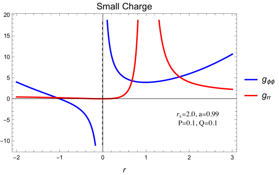
Figure 3: Behavior of $g_{rr}$ and $g_{\phi\phi}$ as functions of radial coordinate $r$ in small charge configuration.

Figure 3, 4 and 5 show the behavior of the metric components $g_{rr}$ and $g_{\phi\phi}$ of the two possible extremal black hole configurations. For the small charge configuration, the horizon is at $r=1.00$, while the CTC boundaries are at $r=-1.0,-0.01$. In the moderate charge configuration, the horizon is at $r=1.00$, while the CTC boundarites are at $r=-1.0,-0.09$. Finally, in the large charge configuration, the horizon is at $r=2.045$, while the CTC boundaries are at $r=-0.332,-0.160,0.045,2.217$. This demonstrates that CTCs always exist in the region behind the extreme DKSBH horizon for all configurations.

IV Relativistic Scalar Field

The dynamics of scalar field $\psi$ in a curved spacetime is described by the following covariant Klein–Gordon equation Derig ; Luzio ,

$$\left[\nabla_{\mu}\nabla^{\mu}-\left(\frac{mc}{\hbar}\right)^{2}\right]\psi=0,$$ (23)

where $\nabla_{\mu}$ is covariant derivative and $m$ is the scalar’s rest mass. It is possible to explicitly express the covariant wave equation in terms of partial derivatives via the Laplace-Beltrami operator as follows,

$$\left[\frac{1}{\sqrt{-g}}\partial_{\mu}\left(\sqrt{-g}\ g^{\mu\nu}\partial_{\nu}\right)-\left(\frac{mc}{\hbar}\right)^{2}\right]\psi=0.$$ (24)

Substituting the metric determinant $g={det}(g_{\mu\nu})$ and the metric inverse $g^{\mu\nu}$ into (24), we obtain this following expression (see Senjaya for derivation details),

$$\left[-\frac{{1}}{\Delta\rho^{2}}\left\{{\left[r\left(r-2d\right)-k^{2}+a^{2}\right]}^{2}-\Delta a^{2}{{\sin}^{2}\theta\ }\right\}{\partial}^{2}_{ct}\right.\\ \left.-2\frac{\left[r\left(r-2d\right)-k^{2}+a^{2}-\Delta\right]a}{\Delta\rho^{2}}{\partial}_{ct}{\partial}_{\phi}\right.\\ \left.+\frac{1}{\rho^{2}}{\partial}_{r}\left(\Delta{\partial}_{r}\right)+\frac{1}{\rho^{2}{\sin\theta\ }}{\partial}_{\theta}\left({\sin\theta\ }{\partial}_{\theta}\right)\right.\\ \left.+\frac{\Delta-a^{2}{{\sin}^{2}\theta\ }}{\Delta{{\sin}^{2}\theta\ }\rho^{2}}{\partial}^{2}_{\phi}\right]\psi-\frac{m^{2}c^{2}}{{\hbar}^{2}}\psi=0.$$ (25)

The expression above is a linear second order differential equation, which depends on the spacetime variables $ct,r,\theta,\phi$. Using the separation ansatz, we can express the scalar field $\psi(ct,r,\theta,\phi)$, taking into account the temporal and azimuthal symmetry Dong ; 35 ,

$$\psi\left(t,r,\theta,\phi\right)=e^{-i\frac{E}{c}ct+im_{\ell}\phi}R\left(r\right)T\left(\theta\right).$$ (26)

Substituting back the ansatz into the main equation (25), followed by multiplying the whole equation by $\rho^{2}r^{2}/\psi\left(t,r,\theta,\phi\right)$, we arrive at this following expression,

$$\left[\frac{1}{T{\sin\theta\ }}{\partial}_{\theta}\left({\sin\theta\ }{\partial}_{\theta}T\right)-\frac{m^{2}_{l}}{{{\sin}^{2}\theta\ }}\right.\\ \left.-\left(\frac{\Omega^{2}_{0}a^{2}}{r^{2}_{s}}-\frac{\Omega^{2}a^{2}}{r^{2}_{s}}\right){{\cos}^{2}\theta\ }\right]+\left[\frac{1}{R}{\partial}_{r}\left(\Delta{\partial}_{r}R\right)\right.\\ \left.+\frac{\Omega^{2}}{r^{2}_{s}}\frac{{\left(r\left(r-2d\right)-k^{2}+a^{2}\right)}^{2}}{\Delta}-\frac{\Omega^{2}a^{2}}{r^{2}_{s}}\right.\\ \left.-2\frac{\left(r\left(r-2d\right)-k^{2}+a^{2}-\Delta\right)a}{\Delta}\left(\frac{\Omega m_{\ell}}{r_{s}}\right)\right.\\ \left.+\frac{m^{2}_{l}a^{2}}{\Delta}-\frac{\Omega^{2}_{0}}{r^{2}_{s}}\left(r\left(r-2d\right)-k^{2}\right)\right]=0,$$ (27)

where we have defined two dimensionless energy parameters,

$$\Omega=\frac{Er_{s}}{\hbar c}\ \ \ ,\ \ \Omega_{0}=\frac{E_{0}r_{s}}{\hbar c}=\frac{(mc^{2})r_{s}}{\hbar c}.$$ (28)

Note that $\Omega_{0}$ can be understood as the inverse ratio of the Compton wavelength of the scalar and the Schwarzschild circumference of the black hole.

IV.1 Polar Sector

The first squared bracket depends only on $\theta$, therefore, can be separated from the rest as follows,

$$\frac{1}{{T\sin\theta\ }}{\partial}_{\theta}\left({\sin\theta\ }{\partial}_{\theta}T\right)-\frac{m^{2}_{\ell}}{{{\sin}^{2}\theta\ }}\\ -\left(\frac{\Omega^{2}_{0}a^{2}}{r^{2}_{s}}-\frac{\Omega^{2}a^{2}}{r^{2}_{s}}\right){{\cos}^{2}\theta\ }=-\lambda^{m_{\ell}}_{\ell},$$ (29)

where $\lambda^{m_{\ell}}_{\ell}$ is the separation constant.

Remark that if $a=0$, $\lambda^{m_{\ell}}_{\ell}=\ell\left(\ell+1\right)$ and the exact solution of the polar sector is given by the associated Legendre polynomial, $P^{m_{\ell}}_{\ell}(\cos\theta)$. If combined with the azimuthal solution, the whole angular solution becomes the Spherical Harmonics.

However, for a general rotating black hole spacetime, the polar equation is expressed as a superposition of the Spherical Harmonics called Spheroidal Harmonics, $S^{m_{\ell}}_{l}$,

$$T(\theta){=}S^{m_{\ell}}_{\ell}\left(\sigma,{\cos\theta\ }\right)=\sum^{\infty}_{r=-\infty}{d^{\ell m_{\ell}}_{r}\left(\sigma\right)P^{m_{\ell}}_{\ell+r}\left({\cos\theta}\right)},$$ (30)

where,

$$\sigma=\frac{\Omega^{2}_{0}a^{2}}{r^{2}_{s}}-\frac{\Omega^{2}a^{2}}{r^{2}_{s}}.$$ (31)

The coefficients $d^{lm_{\ell}}_{r}$ is a constant and act as amplitude of the corresponding mode in the expansion. For the case $\sigma<1$, $\lambda^{m_{\ell}}_{\ell}$ can be calculated perturbatively Press ; Berti1 ; Berti2 ; Cho:2009wf ; Suzuki:1998vy , and expressed in this following expression,

$$\lambda^{m_{\ell}}_{\ell}=\ell(\ell+1)-2\sigma\left(\frac{m_{\ell}^{2}+\ell(\ell+1)-1}{(2\ell-1)(2\ell+3)}\right)+O\left(\sigma^{2}\right).$$ (32)

IV.2 Radial Sector

Replacing the polar sector in the equation (29) by the separation constant $\lambda^{m_{\ell}}_{\ell}$, we are left with the following radial equation,

$${\partial}_{r}\left(\Delta{\partial}_{r}R\right)+\left[\frac{1}{\Delta}{\left\{\frac{\Omega}{r_{s}}\left(r\left(r-2d\right)-k^{2}+a^{2}\right)-m_{\ell}a\right\}}^{2}\right.\\ \left.-\left\{\frac{\Omega^{2}_{0}}{r^{2}_{s}}\left(r\left(r-2d\right)-k^{2}+a^{2}\right)+\frac{\Omega^{2}}{r^{2}_{s}}a^{2}-\frac{\Omega^{2}_{0}}{r^{2}_{s}}a^{2}\right.\right.\\ \left.\left.-2\frac{\Omega m_{\ell}}{r_{s}}a+\lambda^{m_{\ell}}_{\ell}\right\}\right]R{=0},$$ (33)

It is noteworthy that the aforementioned radial equation possesses a general applicability and valid for all scenarios, encompassing sub-extremal, extremal, or super-extremal DKSBHs.

Now, let us focus our invetigation on the extremal DKSBH case. In the extreme condition, where $\delta_{r}=0$, the black hole’s horizons are merged at a position, $r_{H}$, given by equation (11). Therefore, we can rewrite $\Delta=\Delta_{E}$ as follows,

$$\Delta_{E}=(r-r_{H})^{2},$$ (34)

and consequently, we get the following expression of the radial equation in the extremal rotating black hole spacetime,

$${\partial}^{2}_{r}R+\frac{2}{r-r_{H}}{\partial}_{r}R+\left[\frac{1}{{\left(r-r_{H}\right)}^{4}}{\left\{\frac{\Omega}{r_{s}}\left(a^{2}-k^{2}+r\left(r-2d\right)\right)-am_{\ell}\right\}}^{2}\right.\\ \left.-\frac{1}{{\left(r-r_{H}\right)}^{2}}\left\{\frac{{\Omega}^{2}_{0}}{r^{2}_{s}}\left(a^{2}-k^{2}+r\left(r-2d\right)\right)+K^{m_{\ell}}_{\ell}\right\}\right]R=0,$$ (35)

where,

$$K^{m_{\ell}}_{\ell}=\frac{\Omega^{2}}{r^{2}_{s}}a^{2}-\frac{\Omega^{2}_{0}}{r^{2}_{s}}a^{2}-2\frac{\Omega m_{\ell}}{r_{s}}a+\lambda^{m_{\ell}}_{\ell}.$$ (36)

Be defining a new dimensionless radial variable, $\displaystyle{x=\frac{r-r_{H}}{r_{s}}}$, we obtain the following one dimensional Schrödinger-like equation,

$${\partial}^{2}_{x}R+\frac{2}{x}{\partial}_{x}R+V_{eff}\left(x\right)R=0,$$ (37)

The effective potential, $V_{eff}\left(x\right)$, is obtained as follows,

$$V_{eff}\left(x\right)=V_{0}+\frac{V_{1}}{x}+\frac{V_{2}}{x^{2}}+\frac{V_{3}}{x^{3}}+\frac{V_{4}}{x^{4}},$$ (38)

where the coefficient of each term of the $V_{eff}\left(x\right)$ is given as follows,

$${{V}}_{{4}} =\frac{1}{r^{4}_{s}}{\left\{\Omega\left(a^{2}-k^{2}+r_{H}\left(r_{H}-2d\right)\right)-am_{\ell}r_{s}\right\}}^{2}$$

$$=\begin{multlined}{\left\{\Omega-\frac{am_{\ell}r_{s}}{a^{2}-k^{2}+r_{H}\left(r_{H}-2d\right)}\right\}}^{2}\times\\ {\left(\frac{a^{2}-k^{2}+r_{H}\left(r_{H}-2d\right)}{r^{2}_{s}}\right)}^{2}\end{multlined}{\left\{\Omega-\frac{am_{\ell}r_{s}}{a^{2}-k^{2}+r_{H}\left(r_{H}-2d\right)}\right\}}^{2}\times\\ {\left(\frac{a^{2}-k^{2}+r_{H}\left(r_{H}-2d\right)}{r^{2}_{s}}\right)}^{2}$$ (40)

$$={\left\{\Omega-{\Omega}_{c}\right\}}^{2}\zeta^{2}$$

$$={{\Delta}}^{2}_{{\Omega}}{\zeta}^{2},$$ (41)

where we have defined three dimensionless constants,

$${\Delta}_{\Omega}=\Omega-{\Omega}_{c},$$ (42)

$${\Omega}_{c}=\frac{am_{\ell}r_{s}}{a^{2}-k^{2}+r_{H}\left(r_{H}-2d\right)},$$ (43)

$$\zeta=\frac{a^{2}-k^{2}+r_{H}\left(r_{H}-2d\right)}{r^{2}_{s}}.$$ (44)

The coefficient of $x^{-3}$ reads,

$$V_{3} =\begin{multlined}\frac{1}{r^{3}_{s}}\Omega\left(4r_{H}-4d\right)\times\\ \left\{\Omega\left(a^{2}-k^{2}+r_{H}\left(r_{H}-2d\right)\right)-am_{\ell}r_{s}\right\}\end{multlined}\frac{1}{r^{3}_{s}}\Omega\left(4r_{H}-4d\right)\times\\ \left\{\Omega\left(a^{2}-k^{2}+r_{H}\left(r_{H}-2d\right)\right)-am_{\ell}r_{s}\right\}$$ (46)

$$={2}{\Omega}{{\Delta}}_{{\Omega}}\zeta,$$ (47)

where we have used the equation for extremal black hole horizon, $\displaystyle{r_{H}-d=\frac{r_{s}}{2}}$, to obtain the final expression.

The coefficient of $x^{-2}$ after substituting $K^{m_{\ell}}_{\ell}$ as in (36) reads as follows,

$$V_{2}=\frac{1}{r^{2}_{s}}\left\{-r^{2}_{s}{\lambda}^{m_{\ell}}_{\ell}+{\Omega}^{2}_{0}\left(k^{2}-r_{H}\left(r_{H}-2d\right)\right)\right.\\ \left.+{\Omega}^{2}\left(a^{2}+4d^{2}-2k^{2}+6r_{H}\left(r_{H}-2d\right)\right)\right\},$$ (48)

where simplifications can be made,

$$a^{2}+4d^{2}-2k^{2}+6r_{H}\left(r_{H}-2d\right)\\ =2\left(a^{2}-k^{2}+r_{H}\left(r_{H}-2d\right)\right)-a^{2}+4{\left(d-r_{H}\right)}^{2}\\ =2\zeta r^{2}_{s}-a^{2}+4{\left(-\frac{r_{s}}{2}\right)}^{2}=r^{2}_{s}\left(2\zeta+1\right)-a^{2},$$ (49)

and,

$$k^{2}-r_{H}\left(r_{H}-2d\right)=a^{2}-\zeta r^{2}_{s}.$$ (50)

and the final expression of $V_{2}$ is obtained,

$$V_{2}=-\lambda^{m_{\ell}}_{\ell}+\frac{{\Omega}^{2}}{r_{s}^{2}}\left(r^{2}_{s}\left(2\zeta+{1}\right)-a^{2}\right)+\frac{{\Omega}^{2}_{0}}{r_{s}^{2}}\left(a^{2}-\zeta r^{2}_{s}\right).$$ (51)

The last two coefficients need slight simplification and can be presented as follows,

$$V_{1}=-\frac{1}{r_{s}}2\left(d-r_{H}\right)\left(2{\Omega}^{2}-{\Omega}^{2}_{0}\right)=2\Omega^{2}-\Omega^{2}_{0},$$ (52)

$$V_{0}=-\left(\Omega^{2}_{0}-\Omega^{2}\right).$$ (53)

Putting each of the simplified coefficient back into equation (38), we obtain this following compact expression,

$$V_{eff}\left(x\right)=-\left[{\Omega}^{2}_{0}-{\Omega}^{2}\right]+\frac{1}{x}\left[{2}{\Omega}^{2}-{\Omega}^{2}_{0}\right]\\ +\frac{1}{x^{2}}\left[-{\lambda}^{m_{\ell}}_{\ell}+\frac{{\Omega}^{2}}{r_{s}^{2}}\left(r^{2}_{s}\left(2\zeta+1\right)-a^{2}\right)+\frac{{\Omega}^{2}_{0}}{r_{s}^{2}}\left(a^{2}-\zeta r^{2}_{s}\right)\right]\\ +\frac{1}{x^{3}}\left[2\Omega{\Delta}_{\Omega}\zeta\right]+\frac{1}{x^{4}}\left[{\Delta}^{2}_{\Omega}\zeta^{2}\right].$$ (54)

Following the Appendix A, we should substitute $R(x)=\frac{1}{x}{\mathcal{R}}\left(x\right)$ in order to remove the first order derivative and transform the the radial equation (37) into its normal form as follows,

$${\partial}^{2}_{x}{\mathcal{R}}+V_{eff}\left(x\right){\mathcal{R}}=0.$$ (55)

Remark that the normal form of the radial equation above exactly matches the normal form of the Double Confluent Heun equation (84). Therefore, the radial exact solution of the Klein-Gordon equation in the extremal DKSBH (55) can be expressed in terms of the Double Confluent Heun functions as follows,

$$R={e^{\frac{1}{2}\left(\epsilon x-\frac{\gamma}{x}\right)}x^{\frac{\delta}{2}-1}}\times\\ \left[A\ \operatorname{HeunD}\left(\beta,\alpha,\gamma,\delta,\epsilon,x\right)+Be^{\frac{\gamma}{x}-\epsilon x}x^{2-\delta}\times\right.\\ \left.\operatorname{HeunD}\left(-2+\beta+\delta,\alpha-2\epsilon,-\gamma,4-\delta,-\epsilon,x\right)\right].$$ (56)

Now, let us calculate the explicit expressions of the Double Confluent Heun parameters as functions of the scalar and black hole parameters. We compare the two normal forms, (55) and (78).

1. The coefficient of $x^{0}$:

   $$-\left({\Omega}^{2}_{0}-{\Omega}^{2}\right)=-\frac{\epsilon^{2}}{4}\to\epsilon_{\pm}=\pm 2\sqrt{{\Omega}^{2}_{0}-{\Omega}^{2}}.$$ (57)

   For non-zero scalar mass, to determine the correct sign, consider the regularity of the asymptotic behavior of the wave equations (55) and (84) at $x\to-\infty$, as follows,

   $$R(x\to-\infty)\sim e^{\pm\sqrt{{\Omega}^{2}_{0}-{\Omega}^{2}}x}=e^{\epsilon_{\pm}x}\to 0,$$ (58)

   clearly, the correct choice is $\epsilon_{+}$.

2. The coefficient $x^{-4}$:

   $${\Delta}^{2}_{\Omega}{\zeta}^{2}=-\frac{{\gamma}^{2}}{4}\to{\gamma}_{\pm}=\pm 2i{\Delta}_{\Omega}\zeta.$$ (59)

3. The coefficient $x^{-3}$:

   $$2\Omega{\Delta}^{\ }_{\Omega}\zeta ={\gamma}_{\pm}\left(1-\frac{\delta}{2}\right),$$

   $$2\Omega{\Delta}^{\ }_{\Omega}\zeta =\pm 2i{\Delta}_{\Omega}\zeta\left(1-\frac{\delta}{2}\right),$$

   $$\delta =2\left(1\pm i\Omega\right).$$ (60)

4. The coefficient $x^{-1}$:

   $$2{\Omega}^{2}-{\Omega}^{2}_{0} =\alpha-\frac{\epsilon_{+}\delta}{2},$$

   $$2{\Omega}^{2}-{\Omega}^{2}_{0} =\alpha-\frac{2\sqrt{{\Omega}^{2}_{0}-{\Omega}^{2}}\times 2\left(1\pm i\Omega\right)}{2},$$

   $$\alpha =2{\Omega}^{2}-{\Omega}^{2}_{0}+2\left(1\pm i\Omega\right)\sqrt{{\Omega}^{2}_{0}-{\Omega}^{2}}.$$ (61)

5. The coefficient $x^{-2}$:

   $$V_{2}=\frac{\delta}{2}-\frac{\delta^{2}+2\epsilon_{+}\gamma_{\pm}}{4}-\beta,$$ (62)

   $$\begin{multlined}\beta=\lambda^{m_{\ell}}_{\ell}+\Omega\left\{\left(1+\frac{a^{2}-r_{s}^{2}\left(1+2\zeta\right)}{r_{s}^{2}}\right)\Omega\mp i\right\}\\ +(r_{s}^{2}\zeta-a^{2})\frac{\Omega_{0}^{2}}{r_{s}^{2}}\mp 2i\zeta\Delta_{\Omega}\sqrt{\Omega_{0}^{2}-\Omega^{2}}\end{multlined}\beta=\lambda^{m_{\ell}}_{\ell}+\Omega\left\{\left(1+\frac{a^{2}-r_{s}^{2}\left(1+2\zeta\right)}{r_{s}^{2}}\right)\Omega\mp i\right\}\\ +(r_{s}^{2}\zeta-a^{2})\frac{\Omega_{0}^{2}}{r_{s}^{2}}\mp 2i\zeta\Delta_{\Omega}\sqrt{\Omega_{0}^{2}-\Omega^{2}}.$$ (65)

IV.3 Quasiresonance Frequencies

Let us now consider the Double Confluent Heun function’s polynomial condition (86). The regularity of the radial solution at $x\to-\infty$ is ensured by the polynomial condition, which terminates the Frobenius series expansion of the Double Confluent Heun function at order $n$. Furthermore, the formula for calculating the quasiresonance frequency will be derived from the polynomial condition that connects the radial quantum number $n$ to the black hole parameters as well as the scalar mass and energy. Substituting the explicit expression of $\alpha$ and $\epsilon$ into (86) yields,

$$\frac{2{\Omega}^{2}-{\Omega}^{2}_{0}+2\left(1\pm i\Omega\right)\sqrt{{\Omega}^{2}_{0}-{\Omega}^{2}}}{2\sqrt{{\Omega}^{2}_{0}-{\Omega}^{2}}}=-n\ \ ,\ \ n=0,1,\dots$$ (66)

$$\frac{2{\Omega}^{2}-{\Omega}^{2}_{0}}{2\sqrt{{\Omega}^{2}_{0}-{\Omega}^{2}}}\pm i\Omega=-(n+1).$$ (67)

This equation has lengthy analytic solutions which reduces from 3 to 1 solution when subject to the constraint from square root in the denominator. Numerically, it is found that there is only one pure imaginary root.

In Appendix C, we provide an analytic proof that the solution to (67) is purely imaginary for $\Omega_{0}<2$. For $\Omega_{0}\geq 2$, we numerically verify up to very large rest mass that all solutions are still pure imaginary, example plots are shown in Fig. 6. Also note that the sign of the term $\pm i\Omega$ in equation (67) depends on the choice of $\gamma_{\pm}$, i.e., positive (negative) sign for to $\gamma_{+}(\gamma_{-})$ mode. However, the sign will flip for sufficiently large $\Omega_{0}$ (e.g. zeroth mode $n=0$ flips sign at $\Omega_{0}=2$).

Now, let us set $\Omega_{0}=0$ to investigate the quasiresonance frequencies of massless scalar, the energy equation (67) is simplified as follows,

$$\frac{\Omega^{2}}{\pm\sqrt{-\Omega^{2}}}\pm i\Omega=-(n+1),$$ (68)

where the sign in front of $\sqrt{-\Omega^{2}}$ is determined by $\epsilon_{\pm}$ and the sign of $i\Omega$ is determined by $\gamma_{\pm}$.

The equation can be solved algebraically and only $(\epsilon_{+},\gamma_{\pm})$ modes have solutions, shown below,

$$\Omega=\pm\frac{i}{2}\left(1+n\right)\ \ ,\ \ n=0,1,\dots,$$ (69)

where positive (negative) sign corresponds to $\gamma_{+}(\gamma_{-})$ mode. These modes also satisfy Eqn. (58), i.e., the field vanishes at $x\to-\infty$. At the horizon, the asymptotic behavior of the wave (56) at $x\to 0$ becomes

$$R(x\to 0)\sim e^{\mp i\Delta_{\Omega}\frac{\zeta}{x}}.$$ (70)

Using tortoise coordinate defined as

$$r^{*} =\int\frac{r(r-2d)+a^{2}-k^{2}}{(r-r_{H})^{2}}dr,$$

$$r^{*}(r_{H}) \approx\frac{r_{H}(r_{H}-2d)+a^{2}-k^{2}}{-(r-r_{H})}=\frac{\zeta}{-x}.$$ (71)

The near-horizon solution then can be expressed as follows

$$R(x\to 0)\sim e^{\pm i\Delta_{\Omega}r^{*}},$$ (72)

corresponding to outgoing and incoming solution with respect to the horizon respectively. Namely, the $\gamma_{+}~(\gamma_{-}$ modes are the outgoing (incoming) solution to (from) $x\to-\infty$. With respect to the interior region of the black hole, the quasinormal modes (QNMs) are the $\epsilon_{+},\gamma_{+}$ which exponential grows in time while the $\epsilon_{+},\gamma_{-}$ modes are the pure damping modes. The QNMs even having zero real part will enhance and backreact on the interior spacetime behind horizon of the black hole and deform it. The spacetime interior region with the presence of CTCs is unstable with respect to the the scalar perturbation.

In Figure 1 and Figure 2, we plot the quasiresonance frequencies for the first five $\gamma_{+}$ and $\gamma_{-}$ modes respectively with $n=0-4$ against the scalar mass $\Omega_{0}$. All modes are pure imaginary. Notably the zeroth mode $n=0$ changes sign at $\Omega_{0}=2$. Remark that this corresponds to the scalar mass

$$m=\frac{E_{0}}{c^{2}}=\frac{\Omega_{0}\hbar c}{r_{s}c^{2}}=\frac{M_{p}^{2}}{M},$$ (73)

for the Planck mass $M_{p}\equiv\sqrt{\hbar c/G}$. For $M>M_{p}$, we have a hierarchy of mass scale $M_{p}^{2}/M<M_{p}<M$ and the masses are geometrically related. For a solar-mass BH, this mass is $M_{p}^{2}/M=1.34\times 10^{-10}$ eV$/c^{2}$.

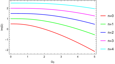
Figure 1: Quasiresonance frequencies for the first five $\epsilon_{+},\gamma_{+}$ modes with $n=0,1,2,3,4$.

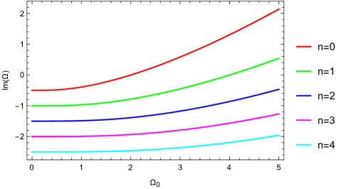
Figure 2: Quasiresonance frequencies for the first five $\epsilon_{+},\gamma_{-}$ modes with $n=0,1,2,3,4$.

The fundamental mode, $n=0$, is the most sensitive to the scalar mass. The higher the excitation, the less sensitive the mode is to the scalar mass. And for $\Omega_{0}\to 0$, we can easily verify the exact formula (69) from the plot.

The $(\epsilon_{+},\gamma_{+})$ modes have purely positive imaginary quasiresonance frequencies in the range $0\leq\Omega_{0}<2$, they grow exponentially, and can destroy the spacetime containing CTCs and decay otherwise. On the other hand, the $\epsilon_{+},\gamma_{-}$ modes have negative imaginary quasiresonance frequencies in the range $0\leq\Omega_{0}<2$ that decay exponentially and grow otherwise. Both modes have zero $Re(\Omega)$, therefore, do not propagate, making it impossible to do time travel. Remark that the positive branch with $0\leq\Omega_{0}<2(n+1)$ and negative branch with $\Omega_{0}>2(n+1)$ has the $n$-th modes $\Omega_{n}$ that grow exponentially and capable of destroying the inner region of spacetime where CTC exists.

V Conclusions and Discussions

In this work, we consider the massive and massless scalar field dynamics in the region behind the horizon of an extremal DKSBH. We begin with a short discussion on the existence of the CTCs in the extremal DKSBH spacetime followed by presenting detailed derivation and novel exact solutions to the Klein-Gordon equation in the extremal charged rotating black hole spacetime. We find that the normal form of the radial Klein-Gordon equation completely matches the normal form of the Double Confluent Heun equation. This enables us to express the exact radial solutions in terms of the Double Confluent Heun function.

The polynomial condition of the Double Confluent Heun function quantizes the energy of the scalar field in the extremal black hole spacetime, resulting in discrete quasiresonance frequencies. We calculate, analyze, and plot the quasiresonance frequencies of both massive and massless scalar fields. The quasiresonance frequencies are double branched, positive and negative pure imaginary, showing no propagating modes, disallow time travel, implying no violation of Hawking’s CPC. The positive branch with $0\leq\Omega_{0}<2(n+1)$ and negative branch with $\Omega_{0}>2(n+1)$, which are growing exponentially, have the potential to backreact, deform and destroy spacetime region with CTCs. An analytic proof that the quasiresonances of the extreme DKSBH are pure imaginary is presented for the scalar mass less than the mass scale $M_{p}^{2}/M$. Numerical consideration for $\Omega_{0}\geq 2$ also confirm that all quasiresonances are pure imaginary, there is no propagating modes inside the extreme DKSBH where CTC exists.

Appendix A Normal Form

The so-called Normal Form of an ordinary differential equation is the form in which an ordinary differential equation is explicitly solved for its maximum derivative. One can begin with the general form of the linear second-order ordinary differential equation as follows,

$$\frac{d^{2}y}{dx^{2}}+p(x)\frac{dy}{dx}+q(x)y=0.$$ (74)

We perform a homotopic transformation through a specific substitution for $y(x)$ that is designed to eliminate the first-order derivative term 2420 , as follows,

$$y=Y(x)e^{-\frac{1}{2}\int{p(x)}dx},$$ (75)

$$\frac{dy}{dx}=\frac{dY}{dx}e^{-\frac{1}{2}\int{p(x)}dx}-\frac{1}{2}Ype^{-\int{p(x)}dx},$$ (76)

$$\frac{d^{2}y}{dx^{2}}=\frac{d^{2}Y}{dx^{2}}e^{-\frac{1}{2}\int{p(x)}dx}-\frac{1}{2}\frac{dY}{dx}pe^{-\frac{1}{2}\int{p(x)}dx}$$

$$-\frac{1}{2}Y\frac{dp}{dx}e^{-\frac{1}{2}\int{p(x)}dx}+\frac{1}{4}Yp^{2}e^{-\frac{1}{2}\int{p(x)}dx}.$$ (77)

Substituting the expressions into (74), we obtain the following normal form,

$$\frac{d^{2}Y}{dx^{2}}+\left(-\frac{1}{2}\frac{dp}{dx}-\frac{1}{4}p^{2}+q\right)Y=0,$$ (78)

and once the solutions to the normal form are obtained, the solutions to the original equation (74) are obtained by substituting $Y(x)$ into (75).

Appendix B The Double Confluent Heun Equation

Very recently, exact radial solutions to the Klein-Gordon equation in the extremal Reissner-Nordström black hole spacetime is discovered and presented in the terms of the Double Confluent Heun functions Senjaya:2024rse . The Double Confluent Heun differential equation is a linear second-order ordinary differential equation with the following canonical form Ish ; Heun ,

$$\frac{d^{2}y}{dx^{2}}+\left(\frac{\gamma}{x^{2}}+\frac{\delta}{x}+\epsilon\right)\frac{dy}{dx}+\left(\frac{\alpha}{x}-\frac{\beta}{x^{2}}\right)y =0.$$ (79)

The differential equation has irregular singular points at $x=0$ and $x=\infty$. Two independent solutions of this equation are given by the Double Confluent Heun functions,

$$y =A\operatorname{HeunD}\left(\beta,\alpha,\gamma,\delta,\epsilon,x\right)+Be^{\frac{\gamma}{x}-\epsilon x}x^{2-\delta}\times$$

$$\phantom{=}\operatorname{HeunD}\left(-2+\beta+\delta,\alpha-2\epsilon,-\gamma,4-\delta,-\epsilon,x\right),$$ (80)

where $\operatorname{HeunD}$ stands for the Double Confluent Heun function.

One can transform the canonical form of the Double Confluent Heun differential equation into its normal form (by following Appendix A) by recognizing,

$$p=\frac{\gamma}{x^{2}}+\frac{\delta}{x}+\epsilon\ \ \ ,\ \ \ q=\frac{\alpha}{x}-\frac{\beta}{x^{2}},$$ (81)

$$y=Y(x)e^{-\frac{1}{2}\left(\epsilon x-\frac{\gamma}{x}\right)}x^{-\frac{\delta}{2}}\equiv\mathcal{H}(x),$$ (82)

and obtain the normal form of (79) as follows,

$$\frac{d^{2}Y}{dx^{2}}+K(x)Y=0,$$ (83)

where,

$$K(x) =-\frac{1}{2}\frac{d{p}}{dx}-\frac{1}{4}{p}^{2}+{q},$$

$$=-\frac{\epsilon^{2}}{4}+\frac{1}{x}\left(-\frac{\epsilon\delta}{2}+\alpha\right)+\frac{1}{x^{2}}\left(\frac{\delta}{2}-\frac{\delta^{2}+2\epsilon\gamma}{4}-\beta\right)$$

$$~~~~~+\frac{1}{x^{3}}\left(\gamma-\frac{\delta\gamma}{2}\right)+\frac{1}{x^{4}}\left(-\frac{\gamma^{2}}{4}\right),$$ (84)

and,

$$Y=e^{\frac{1}{2}\left(\epsilon x-\frac{\gamma}{x}\right)}x^{\frac{\delta}{2}}\times\\ \left[A\operatorname{HeunD}\left(\beta,\alpha,\gamma,\delta,\epsilon,x\right)+Be^{\frac{\gamma}{x}-\epsilon x}x^{2-\delta}\times\right.\\ \left.\operatorname{HeunD}\left(-2+\beta+\delta,\alpha-2\epsilon,-\gamma,4-\delta,-\epsilon,x\right)\right].$$ (85)

The double confluent Heun function becomes polynomial when the following condition is met Ish ,

$$\frac{\alpha}{\epsilon} =-n_{r},\quad n_{r}=0,1,2,\dots.$$ (86)

Appendix C Proof on The Purely Imaginary Quasiresonance

Let us consider the exact formula of the massive scalar quasiresonance frequency in the extremal DKSBH (67). In general, $\Omega$ is complex and can be expressed as $\Omega=z=x+iy$. Substituting the expression into the left-hand side $(l.h.s.)$ of (67) results in this following expression,

$$l.h.s=F_{\pm}(\Omega_{0},x,y)+iG_{\pm}(\Omega_{0},x,y),$$ (87)

where,

$$F_{\pm}=\mp y+\frac{\left(2x^{2}-2y^{2}-\Omega_{0}^{2}\right)\cos\Theta+4xy\sin\Theta}{2\left(x^{4}+2x^{2}\left(y^{2}-\Omega_{0}^{2}\right)+(y^{2}+\ \Omega_{0}^{2})^{2}\right)^{1/4}},$$ (88)

$$G_{\pm}=\pm x+\frac{\left(-2x^{2}+2y^{2}+\Omega_{0}^{2}\right)\sin\Theta+4xy\cos\Theta}{2\left(x^{4}+2x^{2}\left(y^{2}-\Omega_{0}^{2}\right)+(y^{2}+\ \Omega_{0}^{2})^{2}\right)^{1/4}},$$ (89)

$$\Theta=\frac{1}{2}\operatorname{Arg}\left[\Omega_{0}^{2}-(x+iy)^{2}\right].$$ (90)

The right-hand side of (67) is a negative integer, which is strictly real. This implies the imaginary component of the $l.h.s.$ has to be equal to zero,

$$G_{\pm}=0,$$ (91)

and leaving,

$$F_{\pm}=-(n+1)\leq-1.$$ (92)

Therefore, one obvious solution is $x=0,\Omega=iy$, pure imaginary mode.

Remark that the denominator of the second terms can be rearranged as the following,

$$D_{FG}=x^{4}+2x^{2}\left(y^{2}-\Omega_{0}^{2}\right)+(y^{2}+\Omega_{0}^{2})^{2}\\ =(\Omega_{0}^{2}-x^{2})^{2}+y^{2}(2x^{2}+2\Omega_{0}^{2}+y^{2})>0,$$ (93)

and it is obvious that $D_{FG}$ is positive definite.

Now, let us consider $\Theta$,

$$\Theta=\frac{1}{2}\operatorname{Arg}\left[\Omega_{0}^{2}-x^{2}+y^{2}-2ixy\right]=-\frac{1}{2}\tan^{-1}\chi,$$ (94)

$$\Theta^{*}=\frac{1}{2}\operatorname{Arg}\left[\Omega_{0}^{2}-x^{2}+y^{2}+2ixy\right]=\frac{1}{2}\tan^{-1}\chi,$$ (95)

$$\chi=\frac{2xy}{\Omega_{0}^{2}-x^{2}+y^{2}},$$ (96)

where $\chi$ is real and additionally, we also have these following relations,

$$\Theta^{*}=-\Theta,$$ (97)

$$\Theta(-x)=-\Theta(x).$$ (98)

Since $x$ has domain as the following,

$$0\leq x<\Omega_{0},$$ (99)

with $y\ \operatorname{\epsilon}\ \mathcal{R}$, we find $\chi\ \operatorname{\epsilon}\ \mathcal{R}$. However, $\operatorname{tan}^{-1}\chi$ has value ranged between $\left(-\frac{\pi}{2},\frac{\pi}{2}\right)$ and together with the factor $\frac{1}{2}$, $\Theta$ is ranged between $\left(-\frac{\pi}{4},\frac{\pi}{4}\right)$, therefore, we find,

$$\frac{1}{\sqrt{2}}>\cos\Theta\geq 1,$$ (100)

$${\sin\Theta\ }=\left\{\begin{array}[]{c}<0\ \ \ ,\ \ \ y>0\\ >0\ \ \ ,\ \ \ y<0\end{array}\right..$$ (103)

Start with equation (92), it requires $F_{\pm}$ to be less than or equal to $-1$. This condition will also be a constraint for $\{x,y\}$ in each of positive and negative modes. To investigate this, let us explore the derivatives of $F_{\pm}$ as follows,

$$\partial_{x}F_{\pm}=\frac{D_{FG}^{-5/4}}{2}\left[x\left\{(3\Omega_{0}^{2}-2x^{2})(\Omega_{0}^{2}-x^{2})+3y^{2}\Omega_{0}^{2}+2y^{2}(y^{2}+2x^{2})\right\}\cos\Theta\right.\\ \left.+y\left\{(3\Omega_{0}^{2}-2x^{2})(\Omega_{0}^{2}-x^{2})+\Omega_{0}^{2}(2x^{2}+5y^{2})+2y^{2}(y^{2}+2x^{2})\right\}\sin\Theta\right],$$ (104)

$$\partial^{2}_{x}F_{\pm}=\frac{3D_{FG}^{-9/4}}{2}\left[\left\{x^{4}+(\Omega_{0}^{2}+y^{2})^{2}-2x^{2}(\Omega_{0}^{2}+3y^{2})\right\}\cos\Theta+4xy(\Omega_{0}^{2}-x^{2}+y^{2})\sin\Theta\right],$$ (105)

$$\partial_{y}F_{\pm}=\mp 1+\frac{D_{FG}^{-5/4}}{2}\left[x\left\{(3\Omega_{0}^{2}-2x^{2})(\Omega_{0}^{2}-x^{2})+3y^{2}\Omega_{0}^{2}+2y^{2}(y^{2}+2x^{2})\right\}\sin\Theta\right.\\ \left.-y\left\{(3\Omega_{0}^{2}-2x^{2})(\Omega_{0}^{2}-x^{2})+\Omega_{0}^{2}(2x^{2}+5y^{2})+2y^{2}(y^{2}+2x^{2})\right\}\cos\Theta\right],$$ (106)

$$\partial^{2}_{y}F_{\pm}=-\frac{3D_{FG}^{-9/4}}{2}\left[\left\{x^{4}+(\Omega_{0}^{2}+y^{2})^{2}-2x^{2}(\Omega_{0}^{2}+3y^{2})\right\}\cos\Theta+4xy(\Omega_{0}^{2}-x^{2}+y^{2})\sin\Theta\right].$$ (107)

Let us consider $\partial_{x}F_{\pm}$ and $\partial^{2}_{x}F_{\pm}$. It is obvious that the terms in the curly brackets of (104) is definite positive and we can collect this following information,

• The first term inside the square bracket (104) is positive for $x>0$ and zero for $x=0$.

• The second term inside the square bracket (104) is an even function of $y$ and always negative except for $x=0$, where it gives zero.

• Along fixed $y$, $F_{\pm}(x)$ starts off with zero slope at $x=0$,

  $$\partial_{x}F_{\pm}(x=0)=0,$$ (108)

  $$F_{\pm}(x=0)=\mp y-\frac{2y^{2}+\Omega_{0}^{2}}{2(y^{2}+\Omega_{0}^{2})^{1/2}},$$ (109)

  and as $x\to+\infty$, $F_{\pm}(x)$ continuously increases and becomes asymptotically,

  $$\partial_{x}F_{\pm}(x=+\infty)=1,$$ (110)

  $$F_{\pm}(x=+\infty)=\infty.$$ (111)

Based on the above analysis, we can conclude that there is a minimum at $x=0$ for every fixed $y$. The curvature at that point reads,

$$\partial^{2}_{x}F_{\pm}(x=0)=\frac{3\Omega_{0}^{4}}{2(\Omega_{0}^{2}+y^{2})^{5/2}}>0,$$ (112)

allowing us to estimate the shape of $F_{\pm}$ for any constant $y$, i.e., concave upward with respect to $x$.

Now, let us move on to $\partial_{y}F_{\pm}$ and $\partial^{2}_{y}F_{\pm}$,

• The first term inside the square bracket (106) is positive (negative) for $y<0~(y>0)$.

• The second term inside the square bracket (106) is an odd function of $y$ that is positive (negative) for $y>0~(y<0)$.

• Along constant $x$, the positive mode $F_{+}(y)$ begins with zero and zero slope at $y=-\infty$. It reaches $y=0$ with slope $\partial_{y}F_{+}=-1$ and continuously decreases with saturated slope, $\partial_{y}F_{+}=-2$, at $y=+\infty$, where $F_{+}=-\infty$.

• The negative mode, $F_{-}(y)$, starts with $F_{-}=-\infty$ at $y=-\infty$ with saturated slope $\partial_{y}F_{-}=2$. It reaches $y=0$ with slope $\partial_{y}F_{-}=1$ and saturated to zero with zero slope at $y=+\infty$.

It is also straightforward to check that,

$$F_{\pm}(x,0)=\frac{-\Omega_{0}^{2}+2x^{2}}{2\sqrt{\Omega_{0}^{2}-x^{2}}},$$ (113)

is minimized by $x=0$,

$$F_{+}(0,0)=F_{-}(0,0)=-\frac{\Omega_{0}}{2}.$$ (114)

Based on above investigation, we can recap as follows,

• The positive mode, $F_{+}$, is monotonically decreasing in the positive $y$ direction and tends to be flat and zero in the region $y<0$. It fulfills (92) in the region $y>0$.

• The negative mode, $F_{-}$, is monotonically increasing in the positive $y$ direction and tends to be flat and zero in the region $y>0$. It fulfills (92) in the region $y<0$.

• Therefore for $\Omega_{0}<2$ along $x=0$ direction, condition $y>0~(y<0)$ is required for positive (negative) mode to fulfill (92) respectively.

• Remark that equation (113) tells us $F_{\pm}(y)$ is less negative for $x>0$. The positive (negative) modes fulfill (92) later at larger $y>0~(y<0)$. Consequently, the requirement $y>0~(y<0)$ for positive (negative) mode holds for all $x>0$.

After discussing $F_{\pm}$, let us move on to $G_{\pm}$. Along a constant $y$, $G_{\pm}(x)$ is an odd function that is symmetric with respect to $(x\leftrightarrow-x)$. And due to the nature of an odd function, $G_{\pm}(x)$ is always zero at $x=0$. We will show that this is the only solution which satisfies both (91) and (92). It can be done by demonstrating that $G_{\pm}$ has derivatives which do not change signs in the relevant region.

To investigate the behavior of $G_{\pm}(x)$, let us consider its first and second derivatives with respect to $x$ and $y$ as follows,

$$\partial_{x}G_{\pm}=\pm 1+\frac{D_{FG}^{-5/4}}{2}\left[-x\left\{(3\Omega_{0}^{2}-2x^{2})(\Omega_{0}^{2}-x^{2})+3y^{2}\Omega_{0}^{2}+2y^{2}(y^{2}+2x^{2})\right\}\sin\Theta\right.\\ \left.+y\left\{(3\Omega_{0}^{2}-2x^{2})(\Omega_{0}^{2}-x^{2})+\Omega_{0}^{2}(2x^{2}+5y^{2})+2y^{2}(y^{2}+2x^{2})\right\}\cos\Theta\right],$$ (115)

$$\partial^{2}_{x}G_{\pm}=\frac{3D_{FG}^{-9/4}}{2}\left[-\left\{x^{4}+(\Omega_{0}^{2}+y^{2})^{2}-2x^{2}(\Omega_{0}^{2}+3y^{2})\right\}\sin\Theta+4xy(\Omega_{0}^{2}-x^{2}+y^{2})\cos\Theta\right],$$ (116)

$$\partial_{y}G_{\pm}=\frac{D_{FG}^{-5/4}}{2}\left[x\left\{(3\Omega_{0}^{2}-2x^{2})(\Omega_{0}^{2}-x^{2})+3y^{2}\Omega_{0}^{2}+2y^{2}(y^{2}+2x^{2})\right\}\cos\Theta\right.\\ \left.+y\left\{(3\Omega_{0}^{2}-2x^{2})(\Omega_{0}^{2}-x^{2})+\Omega_{0}^{2}(2x^{2}+5y^{2})+2y^{2}(y^{2}+2x^{2})\right\}\sin\Theta\right],$$ (117)

$$\partial^{2}_{y}G_{\pm}=\frac{3D_{FG}^{-9/4}}{2}\left[\left\{x^{4}+(\Omega_{0}^{2}+y^{2})^{2}-2x^{2}(\Omega_{0}^{2}+3y^{2})\right\}\sin\Theta-4xy(\Omega_{0}^{2}-x^{2}+y^{2})\cos\Theta\right].$$ (118)

Let us look into the equation (117). The first term within the square bracket is always positive while the second term is either zero, when $y=0$, or negative otherwise. Therefore, we can estimate the behavior of $\partial_{y}G_{\pm}$ as follows,

• With respect to $y$, if $x=0$, $\partial_{y}G_{\pm}$ is zero for all $y$.

• For each non-zero $x$ in the range $0\ <\ x<\Omega_{0}$, $G_{\pm}$ starts off with a maximum positive slope at $y=0$,

  $$\partial_{y}G_{\pm}(y=0)=\frac{x(3\Omega_{0}^{2}-2x^{2})}{2(\Omega_{0}^{2}-x^{2})^{3/2}}>0,$$ (119)

  with,

  $$\partial^{2}_{y}G_{\pm}(y=0)=0.$$ (120)

• As $|y|$ grows, the negative second term in (117) increases, reducing the slope until $G_{\pm}$ becomes flat at $|y|=\infty$, where the corresponding slope is,

  $$\partial_{y}G_{\pm}(y=\pm\infty)=0.$$ (121)

Namely, $G_{\pm}$ monotonically increases with respect to $y$, from zero slope at $y=-\infty,G_{\pm}=0,-2x$, crosses $y=0$ with $G_{\pm}=\pm x$ and saturates to $G_{\pm}=2x,0$ with zero slope at $y=+\infty$ respectively.

With respect to $x$, for $y>0$, $\partial_{x}G_{+}$ is always positive since $-x\sin\Theta>0$ and $y\cos\Theta>0$ (note that this requires $\Omega_{0}<2$ for $F_{+}$ to satisfy (92)). Thus, $G_{+}(x)$ is monotonically increasing in positive $x$ direction, starts with zero at $x=0$ and continuously climbs up as $x$ increases. Conversely for the negative modes, $\partial_{x}G_{-}$ is always negative for $y<0$ (also this requires $\Omega_{0}<2$ for $F_{-}$ to satisfy (92)) because $-x\sin\Theta<0$ and $y\cos\Theta<0$. $G_{-}$ starts with zero at $x=0$ and continuously drops down as $x$ increases. Therefore, along fixed $y$, the only zero of $G_{\pm}$ is at $x=0$.

Based on these analyses, it can be concluded that there is only one solution for $G_{\pm}$ that satisfies (91), i.e., at $x=0$ for $\Omega_{0}<2$. As a result, for $\Omega_{0}<2$ the quasiresonance frequency is purely imaginary, $\Omega=\pm iy$. For $\Omega_{0}\geq 2$, we numerically explore the solutions and also find that they are strictly pure imaginary as shown in Fig. 6.

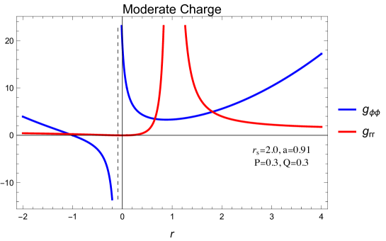
Figure 4: Behavior of $g_{rr}$ and $g_{\phi\phi}$ as functions of radial coordinate $r$ in moderate charge configuration.

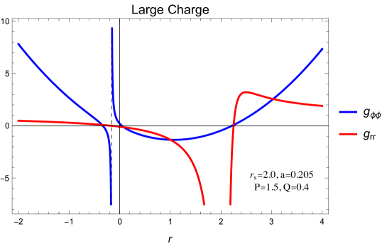
Figure 5: Behavior of $g_{rr}$ and $g_{\phi\phi}$ as functions of radial coordinate $r$ in large charge configuration.

(a)

(b)

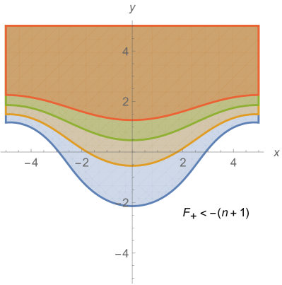
(c)

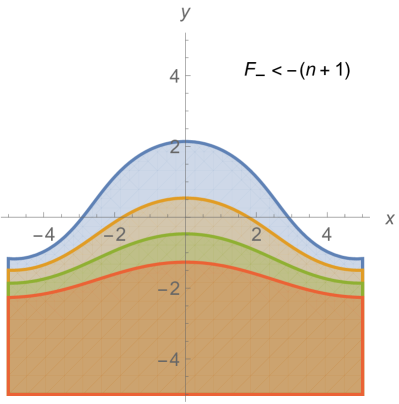
(d)

Figure 6: Region of quasiresonances satisfying (91) and(92) for $\Omega_{0}=5$.

References

- (1) S. W. Hawking, “The Chronology protection conjecture,” Phys. Rev. D 46, 603-611 (1992) doi:10.1103/PhysRevD.46.603
- (2) M. Visser, “From wormhole to time machine: Comments on Hawking’s chronology protection conjecture,” Phys. Rev. D 47, 554-565 (1993) doi:10.1103/PhysRevD.47.554 [arXiv:hep-th/9202090 [hep-th]].
- (3) J. F. Woodward, Found. Phys. Lett. 8, 1-39 (1995) doi:10.1007/BF02187529
- (4) H. a. Shinkai and S. A. Hayward, “Fate of the first traversible wormhole: Black hole collapse or inflationary expansion,” Phys. Rev. D 66, 044005 (2002) doi:10.1103/PhysRevD.66.044005 [arXiv:gr-qc/0205041 [gr-qc]].
- (5) I. D. Novikov and D. I. Novikov, “Collapse of a Wormhole and its Transformation into Black Holes,” J. Exp. Theor. Phys. 129, no.4, 495-502 (2019) doi:10.1134/S1063776119100248
- (6) A. Das, Field Theory: A Path Integral Approach (2nd Edition), World Scientific Publishing Company (2006).
- (7) B. M. Karnakov, V. P. Krainov Field Theory: A Path Integral Approach (2nd Edition), World Scientific Publishing Company (2006).
- (8) S. Chandrasekhar, “The mathematical theory of black holes,” Clarendon Press, 1985, ISBN 978-019-85-0370-5
- (9) T. Bunyaratavej, P. Burikham and D. Senjaya, “Revisiting Chronology Protection Conjecture in The Dyonic Kerr-Sen Black Hole Spacetime,” [arXiv:2408.06023 [gr-qc]].
- (10) M. Richartz, “Quasinormal modes of extremal black holes,” Phys. Rev. D 93, no.6, 064062 (2016) doi:10.1103/PhysRevD.93.064062 [arXiv:1509.04260 [gr-qc]].
- (11) J. Joykutty, “Existence of Zero-Damped Quasinormal Frequencies for Nearly Extremal Black Holes,” Annales Henri Poincare 23, no.12, 4343-4390 (2022) doi:10.1007/s00023-022-01202-z [arXiv:2112.05669 [gr-qc]].
- (12) S. Hod, “Quasi-bound state resonances of charged massive scalar fields in the near-extremal Reissner–Nordström black-hole spacetime,” Eur. Phys. J. C 77, no.5, 351 (2017) doi:10.1140/epjc/s10052-017-4920-8 [arXiv:1705.04726 [hep-th]].
- (13) S. Hod, “Numerical evidence for universality in the relaxation dynamics of near-extremal Kerr–Newman black holes,” Eur. Phys. J. C 75, no.12, 611 (2015) doi:10.1140/epjc/s10052-015-3845-3 [arXiv:1511.05696 [hep-th]].
- (14) P. Burikham, S. Ponglertsakul and T. Wuthicharn, “Quasi-normal modes of near-extremal black holes in generalized spherically symmetric spacetime and strong cosmic censorship conjecture,” Eur. Phys. J. C 80, no.10, 954 (2020) doi:10.1140/epjc/s10052-020-08528-0 [arXiv:2010.05879 [gr-qc]].
- (15) S. Ponglertsakul and B. Gwak, “Massive scalar perturbations on Myers-Perry–de Sitter black holes with a single rotation,” Eur. Phys. J. C 80, no.11, 1023 (2020) doi:10.1140/epjc/s10052-020-08616-1 [arXiv:2007.16108 [gr-qc]].
- (16) D. Wu, S. Q. Wu, P. Wu and H. Yu, “Aspects of the dyonic Kerr-Sen- AdS4 black hole and its ultraspinning version,” Phys. Rev. D 103 (2021) no.4, 044014 doi:10.1103/PhysRevD.103.044014 [arXiv:2010.13518 [gr-qc]].
- (17) S. Jana and S. Kar, “Shadows in dyonic Kerr-Sen black holes,” Phys. Rev. D 108 (2023) no.4, 044008 doi:10.1103/PhysRevD.108.044008 [arXiv:2303.14513 [gr-qc]].
- (18) D. Senjaya, P. Burikham and T. Harko, “The exact relativistic scalar quasibound states of the dyonic Kerr–Sen black hole: quantized energy, and Hawking radiation,” Eur. Phys. J. C 84, no.8, 857 (2024) doi:10.1140/epjc/s10052-024-13225-3 [arXiv:2405.15219 [gr-qc]].
- (19) A. A. Deriglazov and B. F. Rizzuti, “Classical mechanics in reparametrization-invariant formulation and the Schrödinger equation,” Am. J. Phys. 79, 882-885 (2011) doi:10.1119/1.3593270 [arXiv:1105.0313 [math-ph]].
- (20) J. L. Lucio-M, J. A. Nieto, J. D. Vergara, “A generalized Klein-Gordon equation from a reparametrized Lagrangian,“ Phys. Lett. A. 219 (1996), 150-154 doi:0375-9601(96)00456-2
- (21) S. H. Dong, “Wave equations in higher dimensions,” Springer, 2011, ISBN 978-94-007-1916-3 doi:10.1007/978-94-007-1917-0
- (22) W. W. Bell, Special Functions for Scientists and Engineers, Courier Corporation (2004).
- (23) W. H. Press and S. A. Teukolsky, “Perturbations of a Rotating Black Hole. II. Dynamical Stability of the Kerr Metric,” Astrophys. J. 185, 649-674 (1973) doi:10.1086/152445
- (24) E. Berti, V. Cardoso and M. Casals, “Eigenvalues and eigenfunctions of spin-weighted spheroidal harmonics in four and higher dimensions,” Phys. Rev. D 73, 024013 (2006) [erratum: Phys. Rev. D 73, 109902 (2006)] doi:10.1103/PhysRevD.73.109902 [arXiv:gr-qc/0511111 [gr-qc]].
- (25) E. Berti, V. Cardoso and M. Casals, “Eigenvalues and eigenfunctions of spin-weighted spheroidal harmonics in four and higher dimensions,” Phys. Rev. D 73, 024013 (2006) [erratum: Phys. Rev. D 73, 109902 (2006)] doi:10.1103/PhysRevD.73.109902 [arXiv:gr-qc/0511111 [gr-qc]].
- (26) H. T. Cho, A. S. Cornell, J. Doukas and W. Naylor, “Asymptotic iteration method for spheroidal harmonics of higher-dimensional Kerr-(A)dS black holes,” Phys. Rev. D 80, 064022 (2009) doi:10.1103/PhysRevD.80.064022 [arXiv:0904.1867 [gr-qc]].
- (27) H. Suzuki, E. Takasugi and H. Umetsu, “Perturbations of Kerr-de Sitter black hole and Heun’s equations,” Prog. Theor. Phys. 100, 491-505 (1998) doi:10.1143/PTP.100.491 [arXiv:gr-qc/9805064 [gr-qc]].
- (28) G. F. Simmons, Differential Equations with Applications and Historical Notes, CRC Press (2016).
- (29) A. Ronveaux, Heun’s Differential Equations, Clarendon Press (1995).
- (30) D. Senjaya and S. Ponglertsakul, “The extreme Reissner–Nordström Black Hole: New exact solutions to the Klein–Gordon equation with minimal coupling,” Annals Phys. 473, 169898 (2025) doi:10.1016/j.aop.2024.169898 [arXiv:2405.07579 [gr-qc]].
- (31) T. A. Ishkhanyan, V. A. Manukyan, A. H. Harutyunyan and A. M. Ishkhanyan, ”Confluent hypergeometric expansions of the solutions of the double-confluent Heun equation,” Armenian J. Phys. 10, 212-223 (2017)