Riemannian Proximal Sampler
for High-accuracy Sampling on Manifolds

Abstract

We introduce the Riemannian Proximal Sampler, a method for sampling from densities defined on Riemannian manifolds. The performance of this sampler critically depends on two key oracles: the Manifold Brownian Increments (MBI) oracle and the Riemannian Heat-kernel (RHK) oracle. We establish high-accuracy sampling guarantees for the Riemannian Proximal Sampler, showing that generating samples with $\varepsilon$-accuracy requires $\mathcal{O}(\log(1/\varepsilon))$ iterations in Kullback-Leibler divergence assuming access to exact oracles and $\mathcal{O}(\log^{2}(1/\varepsilon))$ iterations in the total variation metric assuming access to sufficiently accurate inexact oracles. Furthermore, we present practical implementations of these oracles by leveraging heat-kernel truncation and Varadhan’s asymptotics. In the latter case, we interpret the Riemannian Proximal Sampler as a discretization of the entropy-regularized Riemannian Proximal Point Method on the associated Wasserstein space. We provide preliminary numerical results that illustrate the effectiveness of the proposed methodology.

1 Introduction

We consider the problem of sampling from a density $\pi^{X}\propto e^{-f}$ defined on a Riemannian manifold $(M,g)$, where $g$ is the metric on the manifold $M$. Here, the density is defined with respect to the volume measure $dV_{g}$ and the normalization constant $\int_{M}e^{-f}dV_{g}<\infty$ is unknown. Riemannian sampling arises in various domains. In Bayesian inference, it is used for sampling from distributions with complex geometries, such as those encountered in hierarchical Bayesian models, latent variable models, and machine learning applications like Bayesian deep learning (Girolami and Calderhead, 2011; Byrne and Girolami, 2013; Patterson and Teh, 2013; Liu and Zhu, 2018; Arnaudon et al., 2019; Liu et al., 2016; Piggott and Solo, 2016; Muniz et al., 2022; Lie et al., 2023). In statistical physics, it plays a crucial role in simulating molecular systems with constrained dynamics (Leimkuhler and Matthews, 2016). Additionally, it appears in optimization problems over manifolds, including eigenvalue problems and low-rank matrix approximations (Goyal and Shetty, 2019; Li and Erdogdu, 2023; Yu et al., 2023; Bonet et al., 2023) and as a module in Riemannian diffusion models (De Bortoli et al., 2022; Huang et al., 2022).

On a Riemannian manifold, Langevin dynamics has the form $dX_{t}=-\operatorname{grad\,}f(X_{t})dt+\sqrt{2}dB_{t}$ where $\operatorname{grad\,}$ represents the Riemannian gradient and $B_{t}$ is the manifold Brownian motion. This formulation extends Euclidean Langevin dynamics by incorporating geometric information through the Riemannian metric, enabling more efficient exploration of curved probability landscapes. Unlike the Euclidean case, discretizing manifold Brownian motion is non-trivial, except in a few special cases. Li and Erdogdu (2023) considered the case of $M\equiv\mathcal{S}^{d}\times\cdots\times\mathcal{S}^{d}$ (i.e., finite product of spheres) and established convergence rates for a simple discretization scheme that discretizes only the drift (gradient term) while requiring exact implementation of manifold Brownian motion increments–feasible on the sphere. Gatmiry and Vempala (2022) extended this approach to general Hessian manifolds, proving convergence results under the same assumption of exact Brownian motion implementation, which is generally infeasible. Both works require the target density to satisfy a logarithmic Sobolev inequality and establish iteration complexity of $\text{poly}(1/\varepsilon)$ to obtain an $\varepsilon$-approximate sample in KL-divergence. However, the reliance on exact Brownian motion increments significantly limits the applicability of the results in Gatmiry and Vempala (2022).

Cheng et al. (2022) studied a practical discretization of Riemannian Langevin diffusion, where both the drift and Brownian motion are discretized. They established an iteration complexity in the 1-Wasserstein distance under a general assumption and in the 2-Wasserstein distance under a more restrictive condition, which can be seen as an analog of log-concavity. Their complexity is of order $\tilde{\mathcal{O}}(1/\varepsilon^{2})$. A key technical challenge is that, in the absence of convexity (e.g., on a compact manifold), establishing contractivity under the Wasserstein distance is nontrivial – even for the continuous-time dynamics. This difficulty is overcome through a second-order expansion of the Jacobi equation Cheng et al. (2022, Lemma 29). Kong and Tao (2024) introduced the Lie-group MCMC sampler for sampling from densities on Lie groups, with a primary focus on accelerating sampling algorithms. Their iteration complexity for the 2-Wasserstein distance are also $\text{poly}(1/\varepsilon)$.

Assumption	Source	Setting	Complexity	Metric
Log-Sobolev Inequality (LSI)	Theorem 6	Exact MBI, Exact RHK	$\tilde{\mathcal{O}}(\log\frac{1}{\varepsilon})$	KL
LSI & Assumption 1	Theorem 8	Inexact MBI, Inexact RHK	$\tilde{\mathcal{O}}(\log^{2}\frac{1}{\varepsilon})$	TV

Table 1: A summary of iteration complexity results in this work. Here, $\varepsilon$ represents the target accuracy. The $\tilde{\mathcal{O}}$ notation hides dependency on all other parameters except for $\varepsilon$.

In comparison to the above works for Riemannian sampling, for the Euclidean case, high-accuracy algorithms, i.e., algorithms with iteration complexity of $O(\text{polylog}(1/\varepsilon))$ are available under various assumptions (that are essentially based on (strong) log-concavity or isoperimetry); see for example Lee et al. (2021); Chen et al. (2022); Fan et al. (2023); He et al. (2024) for such results for the Euclidean proximal sampler and Dwivedi et al. (2019); Chen et al. (2020); Chewi et al. (2021); Lee et al. (2020); Wu et al. (2022); Chen and Gatmiry (2023); Andrieu et al. (2024); Altschuler and Chewi (2024) for various Metropolized algorithms including Metropolis Random Walk (MRW), Metropolis Adjusted Langevin Algorithm (MALA) and Metropolis Hamiltonian Monte Carlo (MHMC).

High-accuracy samplers for constrained (Euclidean) sampling, i.e., when the density is supported on convex set $\mathcal{K}\subseteq\mathbb{R}^{d}$ are established for Hit-and-run and Ball-walk based algorithms under various assumptions (Lovász, 1999; Kannan et al., 2006, 1997); see Kook and Zhang (2025, Section 1.3) for a detailed overview of related works. Kook et al. (2022), proposed Constrained Riemannian Hamiltonian Monte Carlo (CRHMC), and used Implicit Midpoint Method to integrate the Hamiltonian dynamics and established a high-accuracy guarantee for discretized CRHMC. Noble et al. (2023) proposed Barrier Hamiltonian Monte Carlo (BHMC) for constrained sampling, along with its discretizations and established asymptotic results. Kook et al. (2024) proposed the “In-and-Out” sampling algorithm that has high-accuracy guarantees for sampling uniformly on a convex body. Recently Kook and Vempala (2024) obtained state-of-the-art results for sampling from log-concave densities on convex bodies using a proximal sampler designed for this problem. Srinivasan et al. (2024a) and Srinivasan et al. (2024b) showed that a Metropolized version of the Mirror and preconditioned Langevin Algorithm obtains high-accuracy guarantees, respectively, under certain assumptions.

Given the above, the following natural question arises:

Can one develop high-accuracy algorithms for sampling on Riemannian manifolds?

To the best of our knowledge, no prior work exists on providing an affirmative answer to this question. In this work, we develop the Riemannian Proximal Sampler which generalizes the Euclidean Proximal Sampler from Lee et al. (2021). In contrast to the Euclidean case, the algorithm is based on the availability of two oracles: the Manifold Brownian Increment (MBI) oracle and the Riemannian Heat Kernel (RHK) oracle. We show in Theorem 6 that when the exact oracles available the algorithm achieves high-accuracy guarantee in the Kullback-Liebler divergence. Under the availability of inexact oracles, as characterized in Assumption 1, we show in Theorem 8 that the algorithm still achieves high-accuracy guarantees in the total variation metric. Our results are summarized in Table 1. We further develop practical implementations of the aforementioned oracles that satisfy the conditions in Assumption 1 (Section 5), and that are connected to entropy-regularized proximal point method on Wasserstein spaces (Section 6). We also demonstrate the numerical performance of the algorithms via simulations in Appendix A.

2 Preliminaries

We first recall certain preliminaries on Riemannian manifolds; additional preliminaries are provided in Appendix B. We refer the readers to Lee (2018) for more details.

Let $M$ be a Riemannian manifold of dimension $d$ equipped with metric $g$. The manifold $M$ is assumed to be complete, connected Riemannian manifold without boundary. For a point $x\in M$, $T_{x}M$ denotes the tangent space at $x$. For any $v,w\in T_{x}M$, we can write the metric as $g_{x}(v,w)=\langle v,w\rangle_{g}$. For $x\in M$ and $v\in T_{x}M$, $\exp_{x}(v)$ denotes the exponential map. We use $\operatorname{grad\,}$ and $dV_{g}$ to represent the Riemannian gradient and the Riemannian volume form respectively.

For $x\in M$, $\operatorname{Cut\,}(x)$ denotes the cut locus of $x$. For $x,y\in M$, we use $d(x,y)$ to denote the geodesic distance between $x$ and $y$. Let $\operatorname{div\,}$ denotes the Riemannian divergence, and Laplace-Beltrami operator $\Delta:C^{\infty}(M)\to C^{\infty}(M)$ is defined as the Riemannian divergence of Riemannian gradient: $\Delta u=\operatorname{div\,}(\operatorname{grad\,}u)$. We use $\nu(t,x,y)$ to denote the density of manifold Brownian motion with time $t$, starting at $x$, evaluated at $y$.

Let $(M,\mathcal{F})$ be a measurable space. Note that the Riemannian volume form $dV_{g}$ is a measure. A probability measure $\rho$ and its corresponding probability density function $p$ are related through $d\rho=pdV_{g}$. Given a measurable set $A\in\mathcal{F}$, $P_{\rho}(A)$ denotes the probability assigned to the set $A$ by $\rho$. We have $P_{\rho}(A)=\int_{A}p(x)dV_{g}(x)=\int_{A}d\rho(x)$.

Definition 1 (TV distance).

Let $\rho_{1},\rho_{2}$ be probability measures defined on the measurable space $(M,\mathcal{F})$. The total variation distance between $\rho_{1}$ and $\rho_{2}$ is defined as

$$\|\rho_{1}-\rho_{2}\|_{TV}:=\sup_{A\in\mathcal{F}}|\rho_{1}(A)-\rho_{2}(A)|.$$

Definition 2 (KL divergence).

Let $\rho_{1},\rho_{2}$ be probability measures on the measurable space $(M,\mathcal{F})$, with full support. The Kullback-Leibler (KL) divergence of $\rho_{1}$ with respect to $\rho_{2}$ is defined as

$$H_{\rho_{2}}(\rho_{1}):=\int_{M}\log\frac{d\rho_{1}}{d\rho_{2}}d\rho_{1},$$

where $\frac{d\rho_{1}}{d\rho_{2}}$ is the Radon-Nikodym derivative.

It is known that $H_{\rho_{2}}(\rho_{1})\geq 0$ with equality if and only if $\rho_{1}=\rho_{2}$. Although the KL divergence is not symmetric, it serve as a “distance” function between two probability measures. For instance, the well known Pinsker inequality states that $\|\rho_{2}-\rho_{1}\|_{TV}^{2}\leq\frac{1}{2}H_{\rho_{2}}(\rho_{1})$.

Definition 3 (Log-Sobolev Inequality (LSI)).

A probability measure $\rho_{2}$ satisfies Log-Sobolev Inequality with parameter $\alpha>0$ ($\alpha$-$\mathsf{LSI}$) if $H_{\rho_{2}}(\rho_{1})\leq\frac{1}{2\alpha}J_{\rho_{2}}(\rho_{1}),\forall\rho_{1}$, where $J_{\rho_{2}}(\rho_{1}):=\int_{M}\|\operatorname{grad\,}\log\frac{\rho_{1}}{\rho_{2}}\|^{2}d\rho_{1}$ is the relative Fisher information.

For more details on LSI, see Appendix G.2. In Euclidean space, such a condition is a relaxation of strongly convex assumption, and is used to establish convergence of sampling algorithms in KL divergence. See, for example, Vempala and Wibisono (2019) (for the Langevin Monte Carlo Algorithm) and Chen et al. (2022) (for the Euclidean proximal sampler).

2.1 Curvature

We also need notions of curvature on manifolds to present our main results. Let $\mathfrak{X}(M)$ denote the set of all smooth vector fields on $M$. Define a map called Riemann curvature endomorphism by $R:\mathfrak{X}(M)\times\mathfrak{X}(M)\times\mathfrak{X}(M)\to\mathfrak{X}(M)$ by $R(X,Y)Z=\nabla_{X}\nabla_{Y}Z-\nabla_{Y}\nabla_{X}Z-\nabla_{[X,Y]}Z.$ While such definition is very abstract, we provide an intuitive explanation of what curvature is. Intuitively, on a manifold of positive curvature (say, a $2$-dimensional sphere), geodesics tend to “contract”. More precisely, given $x,y\in M$ and $v\in T_{x}M$, we can parallel transport $v$ to $u=P_{x}^{y}v\in T_{y}M$. It is a well-known result that (ignore higher order terms) $d(\exp_{x}tv,\exp_{y}tu)\leq(1-\frac{t^{2}}{2}K)d(x,y)$ for some $K$ (which is actually the sectional curvature). From this, we see that for positive curvature, which means $K>0$, the distance between geodesics would decrease.

Formally, given $v,w\in T_{p}M$ being linearly independent, the sectional curvature of the plane spanned by $v$ and $w$ can be computed through $K(v,w)=\frac{\langle R(v,w)w,v\rangle}{|v|^{2}|w|^{2}-\langle v,w\rangle^{2}}$; see Lee (2018, Proposition 8.29). On the other hand, Ricci curvature can be viewed as the average of sectional curvatures. The Ricci curvature at $x\in M$ along direction $v$ is denoted as $\operatorname{Ric\,}_{x}(v)$, which is equal to the sum of the sectional curvatures of the 2-planes spanned by $(v,b_{i})_{i=2}^{d}$ where $v,b_{2},...,b_{d}$ is an orthonormal basis for $T_{x}M$; see Lee (2018, Proposition 8.32).

We remark that the Ricci curvature is actually a symmetric 2-tensor field defined as the trace of the curvature endomorphism on its first and last indices (Lee, 2018), which sometimes is written as $\operatorname{Ric\,}_{x}(u,v)$ for $u,v\in T_{x}M$. The previous notation is a shorthand of $\operatorname{Ric\,}_{x}(v)=\operatorname{Ric\,}_{x}(v,v)$. When we say Ricci curvature is lower bounded by $\kappa$, we mean $\operatorname{Ric\,}(v,v)\geq\kappa,\forall v\in T_{x}M,\|v\|=1$. We end this subsection through some concrete examples.

1. The hypersphere $\mathcal{S}^{d}$ has constant sectional curvature equal to $1$, and constant Ricci curvature $\operatorname{Ric\,}=(d-1)g,\forall x\in M$ (so that $\operatorname{Ric\,}_{x}(v)=d-1$ for all unit tangent vector $v\in T_{x}M$).

2. For $P_{m}\subseteq\mathbb{R}^{m\times m}$, the manifold of positive definite matrices, its sectional curvatures are in the interval $[-\frac{1}{2},0]$; see, for example, Criscitiello and Boumal (2023). Hence its Ricci curvature is lower bounded by $-\frac{m(m+1)-1}{4}$.

2.2 Brownian Motion on Manifolds

Now we briefly discuss Brownian motion on a Riemannian manifold. Recall that in Euclidean space, Brownian motion is described by the Wiener process. Given $x\in\mathbb{R}^{d}$ and $t>0$, the Brownian motion starting at $x$ with time $t$ has (a Gaussian) density function $\nu(t,x,y)=\frac{1}{(2\pi t)^{d/2}}e^{-\frac{\|x-y\|^{2}}{2t}}$. It solves the heat equation $\frac{\partial}{\partial t}\nu(t,x,y)=\frac{1}{2}\Delta_{y}\nu(t,x,y)$ with initial condition $\nu(0,x,y)=\delta_{x}(y)$.

On a Riemannian manifold, we can describe the density of Brownian motion (heat kernel) through heat equation. Let $B_{x,t}$ be a random variable denoting manifold Brownian motion starting at $x$ with time $t$ and let $\nu(t,x,y)$ be the density of $B_{x,t}$. The Brownian motion density $\nu(t,x,y)$ is then defined as the minimal solution of the following heat equation:

$$\begin{split}\frac{\partial}{\partial t}\nu(t,x,y)=\frac{1}{2}\Delta_{y}\nu(t,x,y)\qquad\text{with}\qquad\nu(0,x,y)=\delta_{x}(y).\end{split}$$

More details can be found in Hsu (2002, Chapter 4). Unlike the Euclidean case, on Riemannian manifold, the heat kernel does not have a closed-form solution in general. However, some properties of the Euclidean hear kernel is preserved on a Riemannian manifold. One such property is the following: Consider $M=\mathbb{R}^{d}$ we have $t\log\nu(t,x,y)=t\log\frac{1}{(2\pi t)^{d/2}}-\frac{\|x-y\|^{2}}{2}$. As $t\to 0$, we get $\lim_{t\to 0}t\log\nu(t,x,y)=-\frac{\|x-y\|^{2}}{2}$. On a Riemannian manifold, we have the following result.

Fact 4 (Varadhan’s asymptotic relation (Hsu, 2002)).

For all $x,y\in M$ with $y\notin\operatorname{Cut\,}(x)$, we have

1. $\underset{t\to 0}{\lim}~t\log\nu(t,x,y)=-\frac{d(x,y)^{2}}{2}$ and $\lim_{t\to 0}t\operatorname{grad\,}_{y}\log\nu(t,x,y)=\exp_{y}^{-1}(x)$.

When evaluation of the heat kernel is required for practical applications, the Varadhan asymptotics aforementioned is used (De Bortoli et al., 2022). We illustrate the above with the following example.

Example 5.

For $M=\mathcal{S}^{1}\subseteq\mathbb{R}^{2}$, the heat kernel for time $t$ only depends on the spherical distance but not specific points. Hence we simply write $\nu_{t}(\varphi)=\nu_{t}(d(x,y))=\nu(t,x,y)$ where $\varphi=d(x,y)$ is the geodesic distance between $x$ and $y$. We have $\nu_{t}(\varphi)=\sum_{n\in\mathbb{Z}}\frac{1}{\sqrt{2\pi t}}\exp(-\frac{(\varphi+2\pi n)^{2}}{2t})$; see, for example, Andersson (2013). Here $t$ represent the time of Brownian motion and $\varphi=d(x,y)$ represent the spherical distance between $x,y$. When $x$ is not too large, terms corresponding to $n=0$ would dominate the sum. Thus we can write $\nu(t,x,y)\approx\frac{1}{\sqrt{2\pi t}}\exp(-\frac{d(x,y)^{2}}{2t})$ which recovers Varadhan’s asymptotics.

Yet another numerical method for evaluating the heat kernel on manifold is truncation method; see, for example, Corstanje et al. (2024, Section 5.1) and De Bortoli et al. (2022). In many cases, the heat-kernel has an infinite series expansion. For example, a power series expansion of heat kernel on hypersphere is given in Zhao and Song (2018, Theorem 1), and more examples can be found in Eltzner et al. (2021, Example 1-5). Similar results are also available for more general manifolds; see, for example, Azangulov et al. (2022) for compact Lie groups and their homogeneous space, and Azangulov et al. (2024) for non-compact symmetric spaces. Hence, a natural approach is to truncate this infinite series at an appropriate level. For example, on $\mathcal{S}^{2}\subseteq\mathbb{R}^{3}$, the heat kernel and its truncation up to the $l$-th term (denoted as $\nu_{l}$) can be written respectively as

$$\nu(t,x,y)=\sum_{i=0}^{\infty}e^{-\frac{i(i+1)t}{2}}\frac{2i+1}{4\pi}P_{i}^{0}(\langle x,y\rangle_{\mathbb{R}^{3}})~~\text{and}~~\nu_{l}(t,x,y)=\sum_{i=0}^{l}e^{-\frac{i(i+1)t}{2}}\frac{2i+1}{4\pi}P_{i}^{0}(\langle x,y\rangle_{\mathbb{R}^{3}}),$$

where $P_{i}^{0}$ are Legendre polynomials.

3 The Riemannian Proximal Sampler

 for $k=0,1,2,...$ do

  Step 1 (MBI): From $x_{k}$, sample $y_{k}\sim\pi^{Y|X}(\cdot,x_{k})$ which is a manifold Brownian increment.

  Step 2 (RHK): From $y_{k}$, sample $x_{k+1}\sim\pi^{X|Y}(\cdot,y_{k})\propto e^{-f(x)}\nu(\eta,x,y_{k})$.

 end for

Algorithm 1 Riemannian Proximal Sampler

We now describe the Riemannian Proximal Sampler, introduced in Algorithm 1. Similar to the Euclidean proximal sampler (Lee et al., 2021), the algorithm has two steps. The first step is sampling from the Manifold Brownian Increment (MBI) oracle. The second step is called the Riemannian Heat-Kernel (RHK) Oracle. Recall that $\nu(\eta,x,y)$ denotes the density of manifold Brownian motion with time $\eta$. Define a joint distribution $\pi_{\eta}(x,y)\propto e^{-f(x)}\nu(\eta,x,y)$. Then, step 2 consists of sampling from the aforementioned distribution. When there is no ambiguity, we omit the step size $\eta$ and simply write $\pi(x,y)\propto e^{-f(x)}\nu(\eta,x,y)$. Algorithm 1 is an idealized algorithm, in the sense that we assume exact access to MBI and RHK oracles. Following Chen et al. (2022), next we provide an intuitive explanation for the algorithm from a diffusion process perspective.

Step 1:

For fixed $x$, we see that $\pi^{Y|X}(\cdot,x)\propto\nu(\eta,x,\cdot)$ which is the density of Brownian motion starting from $x$ for time $\eta$. From this we see that the first step of the algorithm is running forward manifold heat flow: $dZ_{t}=dB_{t}$.

Step 2:

We will illustrate that the second step of the algorithm is running the time-reversed process of the forward process. Consider a stochastic process $Z_{t}:t\geq 0$. When we have observations of $x_{\eta}\sim Z_{\eta}$, we can compute the conditional probability of $Z_{0}$ condition on end point $Z_{\eta}$. We denote $\mu(x_{0}|x_{\eta})$ as the posterior. Bayes Theorem says $\mu(x_{0}|x_{\eta})\propto\mu(x_{0})L(x_{\eta}|x_{0})$, where $\mu(x_{0})$ is the prior guess and the likelihood $L$ depends on the model. We consider the following model (forward heat flow): $dZ_{t}=dB_{t}$ with $Z_{0}\sim\pi^{X}\propto e^{-f(x)}$. Then $\mu(x_{0})=\pi^{X}(x_{0})$ and $L(x_{\eta}|x_{0})=\nu(\eta,x_{0},x_{\eta})$. Thus we get $\mu(x_{0}|x_{\eta})\propto e^{-f(x_{0})}\nu(\eta,x_{0},x_{\eta})$, and we observe that $\mu(x_{0}|x_{\eta})$ is exactly $\pi^{X|Y=x_{\eta}}(x_{0}|x_{\eta})$. For the forward heat flow $dZ_{t}=dB_{t}$ with initialization $Z_{0}\sim\pi^{X}\propto e^{-f(x)}$, there is a well-defined time reversed process $\hat{Z}_{t}^{-}$, which satisfies $(Z_{0},Z_{\eta})\overset{d}{=}(\hat{Z}_{\eta}^{-},\hat{Z}_{0}^{-})$. See Appendix C.2 for more details. Based on this, for the time-reversed process $\hat{Z}_{t}^{-}$, the law of $\hat{Z}_{\eta}^{-}$ condition on $\hat{Z}_{0}^{-}=z$ is the same as the posterior $\mu(x|z)$ discussed previously, i.e., $\pi^{X|Y=z}(x)\propto e^{-f(x)}\nu(\eta,x,z)$. Thus we see that the RHK oracle is, from a diffusion perspective, running the time-reversed process.

Implementing Step 1 and Step 2 is non-trivial on Riemannian manifolds. In Sections  5 and 6 respectively, we discuss two approaches based on heat-kernel truncation and Varadhan’s asymptotics. Furthermore, geodesic random walk (Mangoubi and Smith, 2018; Schwarz et al., 2023) is a popular approach to simulate Manifold Brownian Increments (see Appendix A.1), however to the best of our knowledge (in various metrics of interest) is known only under strong assumptions (Cheng et al., 2022; Mangoubi and Smith, 2018).

4 High-Accuracy Convergence Rates

In this section, we provide the convergence rates for the Riemannian Proximal Sampler (Algorithm 1) assuming that the target density satisfies the LSI assumption. Firstly, note that in (Lee et al., 2021) the analysis of Euclidean Proximal Sampler is done assuming the potential function is strongly convex. However, it is known that on a compact manifold, if a function is geodesically convex, then it has to be a constant. Hence assuming the potential $f$ being geodesically convex is not much meaningful. Recently, Cheng et al. (2022) discussed an analog of log-concave distribution on manifolds. Although their setting works for compact manifolds, it requires the Riemannian Hessian of the potential $f$ to be lower bounded by some curvature-related value, which is still restrictive. Hence, we adopt the setting as in Chen et al. (2022), assuming that the target distribution satisfies the LSI.

In Section 4.1, we consider the case where both steps of Algorithm 1 are implemented exactly, and in Section 4.2, we consider the case when MBI and RHK oracles are inexact. Regarding notation, we let $\rho_{k}^{X}(x)$, $\rho_{k}^{Y}(y)$ denote the law of $x$ and $y$ generated by Algorithm 1 at $k$-th iteration, assuming exact MBI and exact RHK oracles. When the oracles are inexact, we let $\tilde{\rho}_{k}^{X}(x)$, $\tilde{\rho}_{k}^{Y}(y)$ to denote the law of $x$ and $y$ generated by Algorithm 1 at $k$-th iteration.

4.1 Rates with Exact Oracles

Our first result is as follows, with the proof provided in Appendix C.

Theorem 6.

Let $M$ be a Riemannian manifold without boundary, i.e., $\partial M=\emptyset$. Assume $\pi^{X}$ satisfies $\alpha$-$\mathsf{LSI}$. Denote the distribution for the $k$-th iteration of Algorithm 1 as $x_{k}\sim\rho_{k}^{X}$. For any initial distribution $\rho_{0}^{X}$, for all $\eta>0$, we have

$$\begin{split}H_{\pi^{X}}(\rho_{k}^{X})&\leq\frac{H_{\pi^{X}}(\rho_{0}^{X})}{(1+\eta\alpha)^{2k}},\qquad\text{if the Ricci curvature is non-negative,}\\ H_{\pi^{X}}(\rho_{k}^{X})&\leq H_{\pi^{X}}(\rho_{0}^{X})\mathopen{}\mathclose{{\left(\frac{\kappa}{\alpha(e^{\kappa\eta}-1)+\kappa}}}\right)^{2k},\qquad\text{otherwise,}\\ \end{split}$$

where $\kappa$ is the lower bound of Ricci curvature. In case of negative curvature, we have

$$H_{\pi^{X}}(\rho_{k}^{X})\leq\frac{H_{\pi^{X}}(\rho_{0}^{X})}{(1+\eta\alpha)^{2k}},\qquad~\text{if}~~\eta\leq\frac{1}{|\kappa|}.$$

Note that the resulting contraction rate depends on the curvature. If the curvature is non-negative, then we can recover the rate in Euclidean space. But in the case of negative curvature, the rate becomes more complicated, and in order to get the contraction rate as in Euclidean space, we need the step size to be bounded above by some curvature-dependent constant.

The above result provides a high-accuracy guarantee for the Riemannian Proximal Sampler in KL-divergence. To see that, consider the case when the Ricci curvature is non-negative. Note that to achieve $\varepsilon$ accuracy in KL divergence, we need $\frac{H_{\pi^{X}}(\rho_{0}^{X})}{(1+\eta\alpha)^{2k}}=\varepsilon$. Taking $\log$ on both sides, we get $k=\mathcal{O}(\frac{\log(H_{\pi^{X}}(\rho_{0}^{X})/\varepsilon)}{\log(1+\eta\alpha)})$. For small step size $\eta$, we have $\frac{1}{\log(1+\eta\alpha)}=\mathcal{O}(\frac{1}{\eta\alpha})$. Hence $k=\mathcal{O}(\frac{1}{\eta\alpha}\log\frac{H_{\pi^{X}}(\rho_{0}^{X})}{\varepsilon})=\tilde{\mathcal{O}}(\frac{1}{\eta}\log\frac{1}{\varepsilon})$. As $\eta$ does not depend on $\varepsilon$, we see that we need $\tilde{\mathcal{O}}(\log\frac{1}{\varepsilon})$ number of iterations.

There are several challenges in obtaining the aforementioned result for the Riemannian Proximal Sampler. In Euclidean space, when a probability distribution $\pi^{X}$ satisfies $\alpha$-$\mathsf{LSI}$, its propagation along heat flow $\pi^{X}*\mathcal{N}(0,tI_{d})$ satisfies $\alpha_{t}$-$\mathsf{LSI}$, with $\alpha_{t}=\frac{\alpha}{1+\alpha t}$. This fact is very important and leveraged in Chen et al. (2022) for proving their convergence rates. A quantitative generalization of such a fact for Riemannian manifolds is not immediate and we establish the required results in Appendix G.2, following Collet and Malrieu (2008), under the required Ricci curvature assumptions.

4.2 Rates with Inexact Oracles

Recall that Algorithm 1 is an idealized algorithm, where we assumed the availability of the MBI and RHK oracles. Note that given $x\in M$, exact MBI oracle generate samples $y\sim\pi_{\eta}^{Y|X}(\cdot|x)$. And given $y\in M$, exact RHK generate samples $x\sim\pi_{\eta}^{X|Y}(\cdot|y)$. In practice, exactly implementing these oracles could be computationally expensive or even impossible. For the Euclidean case, we emphasize that, as the heat kernel has an explicit closed form density (which is the Gaussian), prior works, for example, Fan et al. (2023), only consider inexact Restricted Gaussian Oracles and control the propagated error along iterations.

In this section, we derive rates of convergence in the setting where both the MBI and RHK oracles are implemented inexactly. Specifically, we assume we are able to approximately implement the MBI oracle by generating $y\sim\hat{\pi}_{\eta}^{Y|X}(\cdot|x)$, and approximately implement the RKH oracle by generating $x\sim\hat{\pi}_{\eta}^{X|Y}(\cdot|y)$, see Assumption 1 below.

Assumption 1.

Denote the output of exact RHK oracle as $\pi_{\eta}^{X|Y}(\cdot|y)$ and inexact RHK oracle as $\hat{\pi}_{\eta}^{X|Y}(\cdot|y)$. Similarly, denote the output of exact MBI oracle as $\pi_{\eta}^{Y|X}(\cdot|x)$ and inexact MBI oracle as $\hat{\pi}_{\eta}^{Y|X}(\cdot|x)$. Let $\zeta_{\mathsf{RHK}}$ and $\zeta_{\mathsf{MBI}}$ be the desired accuracy. We assume that, for inverse step size $\eta^{-1}=\tilde{\mathcal{O}}(\log\frac{1}{\zeta})$, the RHK and MBI oracle implementations can achieve respectively $\|\hat{\pi}_{\eta}^{X|Y}(\cdot|y)-\pi_{\eta}^{X|Y}(\cdot|y)\|_{TV}\leq\zeta_{\mathsf{RHK}},\forall y$, and $\|\hat{\pi}_{\eta}^{Y|X}(\cdot|x)-\pi_{\eta}^{Y|X}(\cdot|x)\|_{TV}\leq\zeta_{\mathsf{MBI}},\forall x$. We then let $\zeta\coloneqq\max\{\zeta_{\mathsf{RHK}},\zeta_{\mathsf{MBI}}\}$.

The need for assuming the step size satisfies $\eta^{-1}=\tilde{\mathcal{O}}(\log\frac{1}{\zeta})$ for the approximation quality is as follows. Recall from the discussion below Theorem 6 that the complexity of Riemannian Proximal Sampler depends on the step size as $\mathcal{O}(\frac{1}{\eta})$. Thus if $\eta$ became too small, for example $\eta^{-1}=\mathcal{O}\mathopen{}\mathclose{{\left(\frac{1}{\varepsilon}}}\right)$, then the overall complexity would be $\operatorname{Poly\,}(\frac{1}{\varepsilon})$, which is not a high-accuracy guarantee.

We also briefly explain the intuition in assuming total variation distance error bound in oracle quality, and postpone the detailed discussion to Section 5. To guarantee a high quality oracle, we need a high quality approximation of heat kernel. As mentioned previously, a popular method is through truncation of infinite series. Theoretically, the $L_{2}$ truncation error can be bounded for compact manifold (Azangulov et al., 2022), which says that the difference between the heat kernel and the approximation of heat kernel are close. This naturally imply an error bound in total variation distance, which motivates us to consider the propagated error in total variation distance.

We first start with a result quantifying the error propagated along iterations, under the availability of inexact oracles. The proof of the following result is provided in Appendix D.

Lemma 7.

Let $\rho_{k}^{X}$ denote the law of $X$ through exact oracle implementation of Algorithm 1, and $\tilde{\rho}_{k}^{X}$ denote the law of $x$ through inexact oracle implementation of Algorithm 1. Under Assumption 1, we have $\|\rho_{k}^{X}(x)-\tilde{\rho}_{k}^{X}(x)\|_{TV}\leq k(\zeta_{\mathsf{RHK}}+\zeta_{\mathsf{MBI}})$.

Based on this result, we next obtain the following result analogues to Theorem 6; the proof is provided in Appendix D.

Theorem 8.

Similar to Theorem 6, let $M$ be a Riemannian manifold without boundary and let $\pi^{X}$ satisfies LSI with constant $\alpha$. Further let Assumption 1 hold. For any initial distribution $\rho_{0}^{X}$, to reach $\tilde{\mathcal{O}}(\varepsilon)$ total variation distance with oracle accuracy $\zeta=\zeta_{\mathsf{RHK}}=\zeta_{\mathsf{MBI}}=\frac{\varepsilon}{\log^{2}\frac{1}{\varepsilon}}$ and step size $\frac{1}{\eta}=\tilde{\mathcal{O}}(\log\frac{1}{\varepsilon})$, we need $k=\tilde{\mathcal{O}}(\log^{2}\frac{1}{\varepsilon})$ iterations.

5 Implementation of Inexact Oracles via Heat Kernel Trucation

Theorem 8 shows that as long we have sufficient accuracy of MBI and RHK oracles satisfying Assumption 1, we can have a high-accuracy Riemannian sampling algorithm. In this section, we introduce an approximate implementation, based on heat kernel truncation (as introduced in 2) and rejection sampling. Numerical simulations for this approach are provided in Appendix A.2.

First note that for rejection sampling method (in general) there are two key ingredients: a proposal distribution and an acceptance rate. Assume we want to generate samples from $\rho$ through rejection sampling. We choose a suitable proposal distribution denoted as $\mu$, and a suitable scaling constant $K$ such that the acceptance rate $K\frac{\rho(x)}{\mu(x)}\leq 1,\forall x$. We generate a random proposal $x\sim\mu$ and $u\in[0,1]$ being a uniform random number. Then we compute $K\frac{\rho(x)}{\mu(x)}$, and accept $x$ if $u\leq K\frac{\rho(x)}{\mu(x)}$.

We also introduce the following definition of Riemannian Gaussian distribution, as defined next, which will be used as the proposal distribution in rejection sampling. A Riemannian Gaussian distribution centered at $x^{*}$ with variable $t$ is $\mu(t,x^{*},x)\propto\mu_{u}(t,x^{*},x):=\exp\mathopen{}\mathclose{{\left(-\frac{d(x^{*},x)^{2}}{2t}}}\right)$, where $\mu_{u}$ denote an unnormalized version of $\mu$. We use this as our proposal distribution to implement rejection sampling, as exact sampling from such a distribution is well-studied for certain specific manifolds; see, for example, Said et al. (2017) for symmetric spaces and Chakraborty and Vemuri (2019) for Stiefel manifolds. Furthermore, this notion of a Riemannian Gaussian distribution is also used in the study of differential privacy on Riemannian manifolds due to their practical feasibility (Reimherr et al., 2021; Jiang et al., 2023).

5.1 Implementation of RHK

We first recall the rejection sampling implementation of Restricted Gaussian Oracle (RGO) in the Euclidean setting. Note that, we have $\log\nu_{u}(\eta,x,y_{k})=-\frac{1}{2\eta}\|x-y_{k}\|^{2}$, where $\nu_{u}=\exp(-\frac{1}{2\eta}\|x-y_{k}\|^{2})$ is an unnormalized heat kernel (or the Gaussian density) in Euclidean space. Then we have $\pi_{\eta}^{X|Y}(\cdot,y_{k})\propto e^{-f(x)-\frac{1}{2\eta}\|x-y_{k}\|^{2}}$. Then, the RGO is implemented through rejection sampling. Specifically, we can first find the minimizer $x^{*}\in\operatorname*{arg\,min}_{x}f(x)+\frac{1}{2\eta}\|x-y_{k}\|^{2}$. Note that the minimizer represents the mode of $\pi_{\eta}^{X|Y}(\cdot,y_{k})$. We can then sample a Gaussian proposal $x_{p}\sim\mathcal{N}(x^{*},tI_{d})$ for suitable $t$ centered at the mode $x^{*}$ and perform rejection sampling. For more details, see, for example, Chewi (2023).

On a Riemannian manifold with $\nu$ denoting the heat kernel, to sample from $\pi_{\eta}^{X|Y}(\cdot,y_{k})\propto e^{-f(x)}\nu(\eta,x,y_{k})$ through rejection sampling, we need evaluations of $f(x)-\log\nu(\eta,x,y_{k})$. But in general, we cannot evaluate the heat kernel exactly, hence we seek for certain heat kernel approximations. Hence, we use the truncated heat kernel $\nu_{l}$ to replace $\nu$, and perform rejection sampling, see Algorithm 2. In the rejection sampling algorithm, as mentioned previously, we use a Riemannian Gaussian distribution as the proposal for rejection sampling. We choose suitable step size $\eta$ and $t$ that depends on $\eta$ s.t. $g(x)-g(x^{*})\geq\frac{1}{2t}d(x,x^{*})^{2}$. Such an inequality can guarantee that the acceptance rate (with Riemannian Gaussian distribution $\mu(t,x^{*},x)$ as proposal) would not exceed one, i.e., $\frac{\exp(-g(x)+g(x^{*}))}{\mu_{u}(t,x^{*},x)}\leq 1,\forall x$. Then we see that the output of rejection sampling would follow $\hat{\pi}_{\eta}^{X|Y}(x|y_{k})\propto\exp(f(x)-\log\nu_{l}(\eta,x,y_{k}))$. Similarly, to implement the MBI oracle, we also use rejection sampling to get a high-accuracy approximation. Specifically, Algorithm 3 generates inexact Brownian motion starting from $x$ with time $\eta$.

 Find the minimizer of $g(x):=f(x)-\log\nu_{l}(\eta,x,y_{k})$, denote as $x^{*}$.

 Set suitable $t$ and constant $C_{\mathsf{RHK}}$ s.t. $V_{\mathsf{RHK}}(x):=\frac{\exp(-g(x)+g(x^{*})+C_{\mathsf{RHK}})}{\exp(-\frac{1}{2t}d(x,x^{*})^{2})}\leq 1,\forall x\in M$

 for $i=0,1,2,...$ do

  Generate proposal $x\sim\mu(t,x^{*},\cdot)$.

  Generate $u$ uniformly on $[0,1]$.

  Return $x$ if $u\leq V_{\mathsf{RHK}}(x)$

 end for

Algorithm 2 RHK through Rejection Sampling

 Set suitable $t$ and $C_{\mathsf{MBI}}$ so that $V_{\mathsf{MBI}}(y):=\frac{\exp(\log\nu_{l}(\eta,x,y)-\log\nu_{l}(\eta,x,x)+C_{\mathsf{MBI}})}{\exp(-\frac{d(x,y)^{2}}{2t})}\leq 1,\forall y\in M$

 for $i=0,1,2,...$ do

  Generate proposal $y\sim\mu(t,x,\cdot)$.

  Generate $u$ uniformly on $[0,1]$.

  Return $y$ if $u\leq V_{\mathsf{MBI}}(y)$

 end for

Algorithm 3 MBI through Rejection Sampling

5.2 Verification of Assumption 1

We now show that Assumption 1 is satisfied for the aforementioned inexact implementation of the Riemannian Proximal Sampler. To do so, we specifically consider the case when the manifold $M$ is compact and is a homogeneous space. Recall that $\nu_{l}$ denote the truncated heat kernel with truncation level $l$. Roughly speaking, a homogeneous space is a manifold that has certain symmetry, including Stiefel manifold, Grassmann manifold, hypersphere, and manifold of positive definite matrices.

Proposition 9.

Let $M$ be a compact manifold. Assume further that $M$ is a homogeneous space. With truncation implementation of inexact oracles, in order for Assumption 1 to be satisfied with $\zeta=\frac{\varepsilon}{\log^{2}\frac{1}{\varepsilon}}$, we need truncation level $l$ to be of order $\textrm{polylog}({1}/{\varepsilon})$.

Sketch of proof: We briefly mention the idea of proof. Azangulov et al. (2022, Proposition 21) provided an $L_{2}$ bound on the truncation error, and by Jensen’s inequality we get an $L_{1}$ bound as desired. With truncation level $l$ to be of order $\operatorname{Poly\,}(\log\frac{1}{\varepsilon})$, we can achieve $\int_{M}|\nu(\eta,x,y)-\nu_{l}(\eta,x,y)|dV_{g}(x)=\tilde{\mathcal{O}}(\zeta)$. See Proposition 18 and Proposition 21 for a complete proof.

Remark. In Appendix E.2, we show that on hypersphere $\mathcal{S}^{d}$, when the acceptance rate $V$ in rejection sampling would possibly exceed $1$ in some unimportant region, Assumption 1 still holds, via explicit computations.

When $M$ is not a homogeneous space, to the best of our knowledge, it is unknown how to implement the truncation method. Exploring this direction to further extend the above result is an interesting direction for future work.

6 Implementation via Varadhan’s Asymptotics and Connection to Entropy-Regularized JKO Scheme

In this section, we consider yet another approximation scheme for implementing Algorithm 1, motivated by its connection with the proximal point method in optimization, where the latter is in the sense of optimization over Wasserstein space (Jordan et al., 1998; Wibisono, 2018; Chen et al., 2022). Note that the proximal point method is usually called as the JKO scheme after the authors of Jordan et al. (1998).

Specifically, we consider approximating the heat kernel through Varadhan’s asymptotics. Let $\hat{\nu}(\eta,x,y)\propto_{y}\exp(-\frac{d(x,y)^{2}}{2\eta})=:\hat{\nu}_{u}(\eta,x,y)$ be an inexact evaluation of heat kernel. According to Varadhan’s asymptotics, $\lim_{\eta\to 0}\hat{\nu}(\eta,x,y)=\nu(\eta,x,y)$. Hence when $\eta$ is small, $\hat{\nu}$ is a good approximation of the heat kernel. Note that $\hat{\nu}(\eta,x,\cdot)$ in Varadhan’s asymptotic is exactly the Riemannian Gaussian distribution $\mu(\eta,x,\cdot)$. Denote $\tilde{\pi}(x,y)=\exp(-f(x)-\frac{d(x,y)^{2}}{2\eta})$. With inexact MBI implemented through Riemannian Gaussian distribution and inexact RHK implemented through rejection sampling (Algorithm 2) to generate $\tilde{\pi}^{X|Y}(x|y)\propto\exp(-f(x)-\frac{d(x,y)^{2}}{2\eta})$, we obtain Algorithm 4.

For the case when $M=\mathcal{S}^{d}$, we prove in Appendix G.4 that to sample from $\tilde{\pi}^{X|Y}(x|y)$ through rejection sampling, with suitable parameters, the cost is $\mathcal{O}(1)$ in both dimension $d$ and step size $\eta$. Obtaining similar results for more general manifolds seems non-trivial. Numerical simulations for this approach are provided in Appendix A.3. Verifying Assumption 1 for this implementation is open.

 for $k=0,1,2,...$ do

  From $x_{k}$, sample $y_{k}\sim\tilde{\pi}^{Y|X}(\cdot,x_{k})$ which is a Riemannian Gaussian distribution.

  From $y_{k}$, sample $x_{k+1}\sim\tilde{\pi}^{X|Y}(\cdot,y_{k})\propto e^{-f(x)-\frac{d(x,y_{k}^{2})}{2\eta}}$ using Algorithm 2.

 end for

Algorithm 4 Inexact Manifold Proximal Sampler with Varadhan’s Asymptotics

6.1 RHK as a proximal operator on Wasserstein space

We first show that the inexact RHK output in Algorithm 4 can be viewed as a proximal operator on Wasserstein space, generalizing the Euclidean result in Chen et al. (2020) to the Riemannian setting. Recall that with a function $f$ and $d$ being a distance function, $\operatorname{prox\,}_{\eta f}(y)=\operatorname*{arg\,min}_{x}f(x)+\frac{1}{2\eta}d(x,y)^{2}$. The (approximated) joint distribution is $\tilde{\pi}(x,y)=\exp(-f(x)-\frac{d(x,y)^{2}}{2\eta})$. By direct computation we have the following Lemma (proved in Appendix F).

Lemma 10.

We have that

$$\tilde{\pi}^{X|Y=y}=\operatorname*{arg\,min}_{\rho\in\mathcal{P}_{2}(M)}H_{\tilde{\pi}^{X}}(\rho)+\frac{1}{2\eta}W_{2}^{2}(\rho,\delta_{y})=\operatorname{prox\,}_{\eta H_{\tilde{\pi}^{X}}}(\delta_{y}),$$

which shows that the ineact RHK implementation is a proximal operator, i.e., $\tilde{\pi}^{X|Y=y}=\operatorname{prox\,}_{\eta H_{\tilde{\pi}^{X}}}(\delta_{y})$.

6.2 Connection to Entropy-Regularized JKO Scheme

Observe that in Algorithm 4, the Riemannian Gaussian involves distance square, which naturally relates to Wasserstein distance. Now, recall that for a function $F$ in the Wasserstein space, its Wasserstein gradient flow can be approximated through the following discrete time JKO scheme (Jordan et al., 1998):

$$\rho_{k+1}=\operatorname*{arg\,min}_{\rho\in\mathcal{P}(\mathbb{R}^{d})}F(\rho)+\frac{1}{2\eta}W_{2}^{2}(\rho,\rho_{k}).$$

It was proved that as $\eta\to 0$, the discrete time sequence $\{\rho_{k}\}$ converge to the Wasserstein gradient flow of $F$. Later, Peyré (2015) proposed an approximation scheme through entropic smoothing of Wasserstein distance:

$$\rho_{k+1}=\operatorname*{arg\,min}_{\rho\in\mathcal{P}(\mathbb{R}^{d})}F(\rho)+\frac{1}{2\eta}W_{2,\varepsilon}^{2}(\rho,\rho_{k}),$$

where $W_{2,\varepsilon}$ is the entropy-regularized 2-Wasserstein distance defined by (here $H$ is the negative entropy)

$$W_{2,t}^{2}(\rho_{1},\rho_{2})=\inf_{\gamma\in\mathcal{C}(\rho_{1},\rho_{2})}\int d(x,y)^{2}d\gamma(x,y)+tH(\gamma).$$

In Euclidean space, Chen et al. (2022) showed that the proximal sampler can be viewed as an entropy-regularized JKO scheme. We extend such an interpretation to Riemannian manifolds. Specifically, we show that Algorithm 4 which is an approximation of the exact proximal sampler (Algorithm 1), can be viewed as an entropy-regularized JKO as stated in Theorem 11 (proved in Appendix F). Note that on a Riemannian manifold the negative entropy is $H(\gamma):=\int_{M\times M}\gamma\log(\gamma)dV_{g}(x)dV_{g}(y)$.

Theorem 11.

Recall that $\pi^{X}\propto e^{-f}$. Let $x_{k},y_{k},x_{k+1}$ be generated by Algorithm 4. Let $\tilde{\rho}_{k}^{X}$, $\tilde{\rho}_{k}^{Y}$ and $\tilde{\rho}_{k+1}^{X}$ be the distribution of $x_{k},y_{k},x_{k+1}$, respectively. Then

$$\tilde{\rho}_{k}^{Y}=\operatorname*{arg\,min}_{\chi\in\mathcal{P}_{2}(M)}\frac{1}{2\eta}W_{2,2\eta}^{2}(\tilde{\rho}_{k}^{X},\chi)\quad\text{and}\quad\tilde{\rho}_{k+1}^{X}=\operatorname*{arg\,min}_{\chi\in\mathcal{P}_{2}(M)}\int fd\chi+\frac{1}{2\eta}W_{2,2\eta}^{2}(\tilde{\rho}_{k}^{Y},\chi).$$

7 Conclusion

We introduced the Riemannian Proximal Sampler for sampling from densities on Riemannian manifolds. By leveraging the Manifold Brownian Increments (MBI) and the Riemannian Heat-kernel (RHK) oracles, we established high-accuracy sampling guarantees, demonstrating a logarithmic dependence on the inverse accuracy parameter (i.e., $\text{polylog}(1/\varepsilon)$) in the Kullback-Leibler divergence (for exact oracles) and total variation metric (for inexact oracles). Additionally, we proposed practical implementations of these oracles using heat-kernel truncation and Varadhan’s asymptotics, providing a connection between our sampling method and the Riemannian Proximal Point Method.

Future works include: (i) characterizing the precise dependency on other problem parameters apart from $\varepsilon$, (ii) improving oracle approximations for enhanced computational efficiency and (iii) extending these techniques to broader classes of manifolds (and other metric-measure spaces).

Appendix A Simulation Results

A.1 Brownian Motion Approximation via Geodesic random walk

In our experiments, to compare against the Riemannian Langevin Algorithm, we used the geodesic random walk algorithm to simulate the MBI oracle following Cheng et al. [2022], De Bortoli et al. [2022], Schwarz et al. [2023]; see Algorithm 5. More efficient implementation is a topic of great interest in the literature; see, for example, [Schwarz et al., 2023].

 Input $x\in M,t>0$.

 Sample $\xi$ being a Euclidean Brownian increment with time $t$ in the tangent space $T_{x}M$.

 Output $y=\exp_{x}(\xi)$.

Algorithm 5 Approximation of Manifold Brownian Motion Using Geodesic Random Walk

While it is well-known that geodesic random walks converge asymptotically to the Brownian motion on the manifold, non-asymptotic rates of convergence in various metrics of interest is largely unknown. A basic non-asymptotic error bound for geodesic random walk is available in Wasserstein distance (see Cheng et al. [2022, Lemma 7]). Mixing time results are provided in Mangoubi and Smith [2018]. However, such a result is not immediately applicable to establish high-accuracy guarantees for the Riemannian proximal sampler, when the MBI oracle is implemented via geodesic random walk. An important and interesting future work is establishing rates of convergence for geodesic random walk in various metrics of interest so that those results could be leveraged to obtain high-accuracy guarantees for the Riemannian proximal sampler.

A.2 Numerical Experiments for Algorithms 2 and 3: von Mises-Fisher distribution on Hyperspheres

In this experiment, we test the performance of Algorithms 2 and 3 for sampling from the von Mises-Fisher distribution on hyperspheres and compare it with the Riemannian LMC method. In this case, we have $f(x)=-\kappa\mu^{T}x$. Note that this $f(x)$ has a unique minimizer on $\mathcal{S}^{d}$. This implies that LSI is satisfied, see [Li and Erdogdu, 2023, Theorem 3.4]. We demonstrate the performance of our Algorithm on $\mathcal{S}^{2}\subseteq\mathbb{R}^{3}$ with $\mu=(10,0.1,2)^{T}$ and $\kappa=10$, and on $\mathcal{S}^{5}$ with $\mu=(5,0.1,2,1,1,1)^{T}$ and $\kappa=10$. For the purpose of numerical demonstration, we sample the Riemannian Gaussian distribution through rejection sampling.

To evaluate the performance, we estimate $\mathbb{E}[d(x,x^{*})^{2}]$, where $x^{*}$ is the minimizer of $f$, representing the mode of the distribution, and plot it as a function of iterations. Note that the quantity $\mathbb{E}[d(x,x^{*})^{2}]$ is referred to as Fréchet variance Fréchet [1948], Dubey and Müller [2019]. For this, we generate $10000$ samples (by generating samples independently via different runs) and compute $\frac{1}{10000}\sum_{i=1}^{10000}d(x_{i},x^{*})^{2}$. We use rejection sampling to generate unbiased samples and get an estimation of the true value. Due to the biased nature of the Riemannian LMC method, to achieve a high accuracy we need a small step size. Contrary to the Riemanian LMC method, the proximal sampler is unbiased, and it can achieve an accuracy while using a large step size and a smaller number of iterations; see Figures 1-(a) and (b).

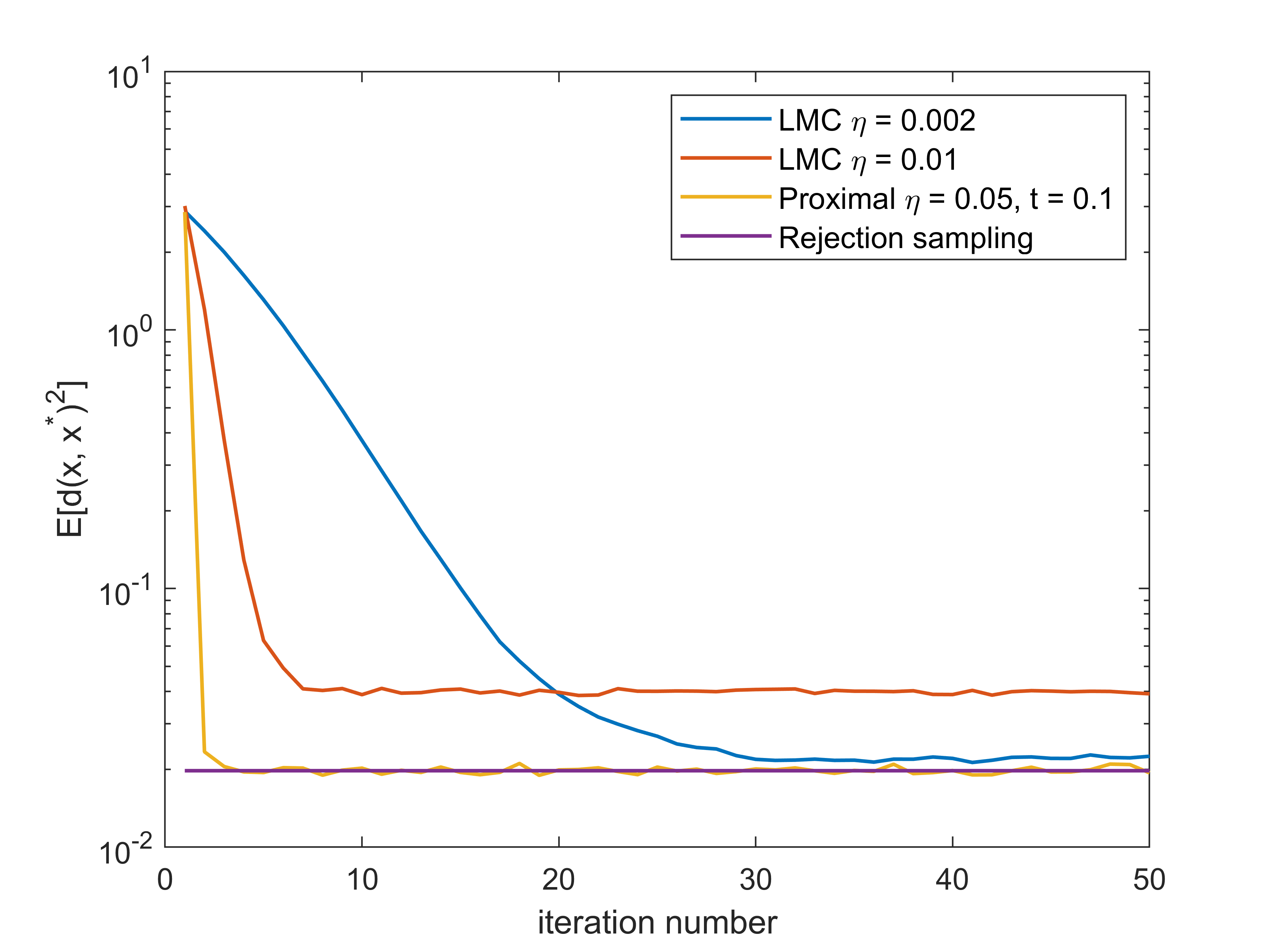
(a) $\mathcal{S}^{2}$, $f(x)=\exp(\kappa\mu^{T}x)$

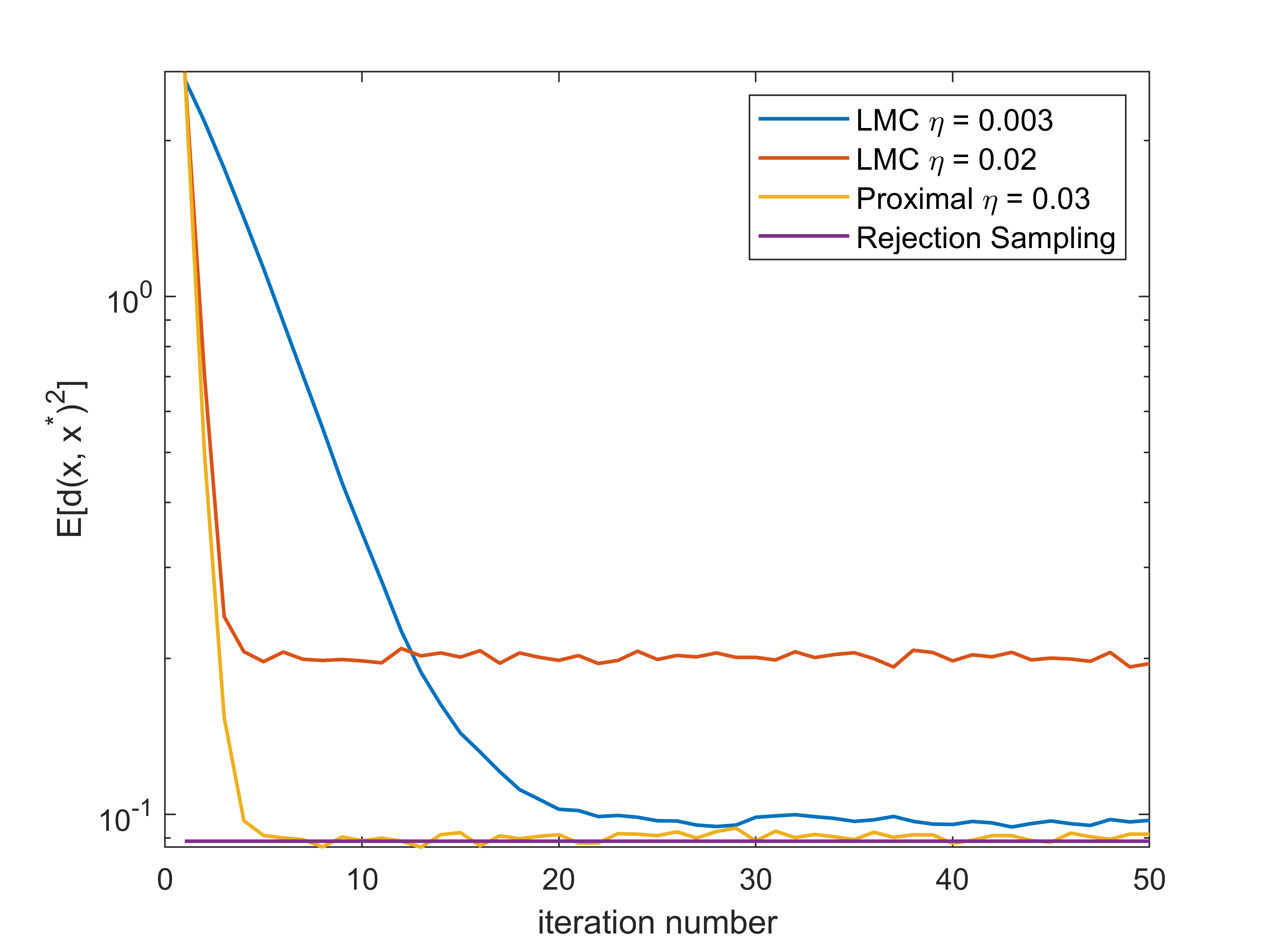
(b) $\mathcal{S}^{5}$, $f(x)=\exp(\kappa\mu^{T}x)$

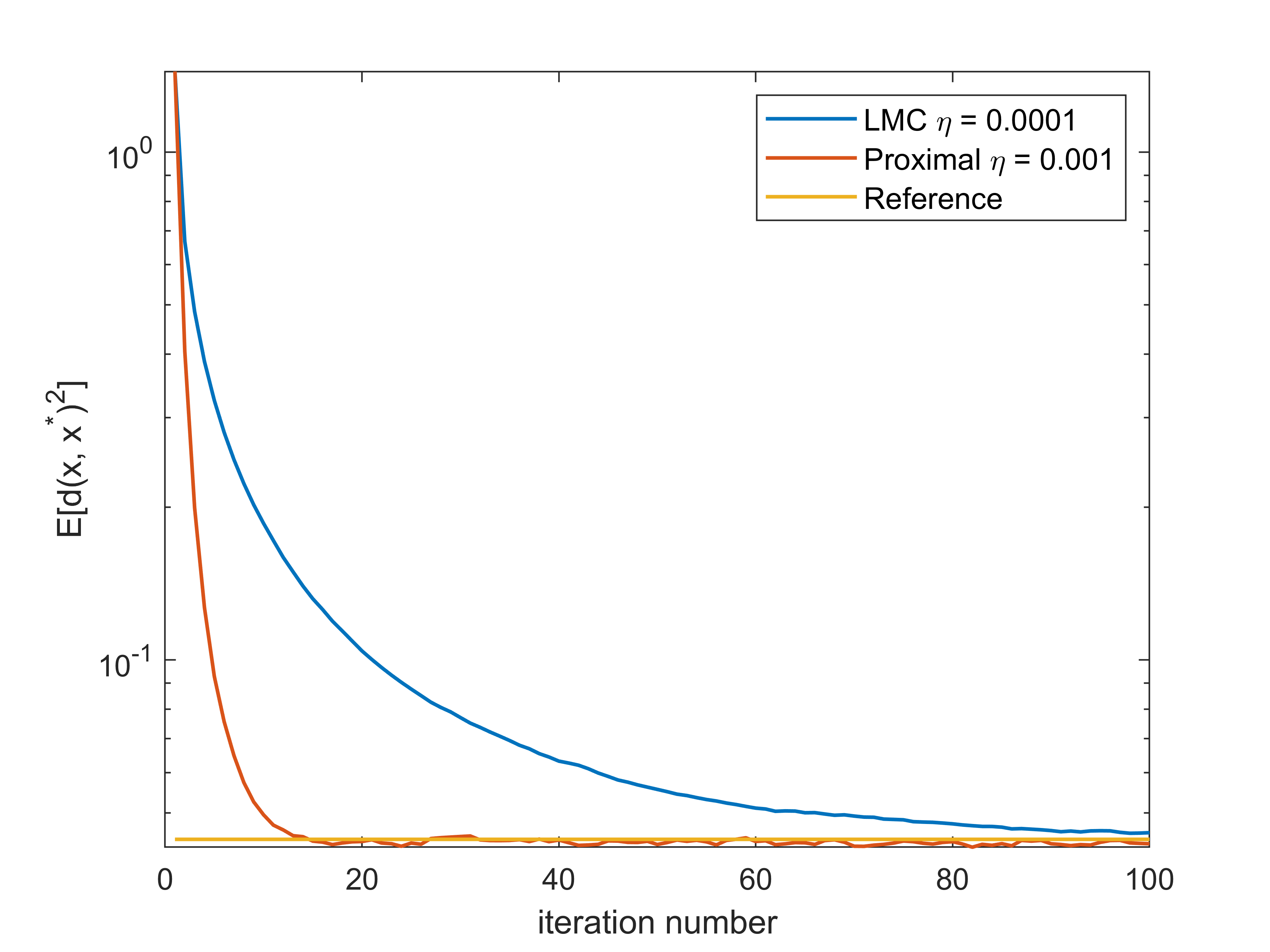
(c) $P_{3}$, $f(X)=\exp(\frac{-d(X,I)^{4}}{2\sigma^{2}})$,

Figure 1: Frechét variance (i.e., $\mathbb{E}[d(x,x^{*})^{2}]$ versus number of iterations. Left and Middle figure correspond to the implementation via Algorithm 2 and 3. Right figure corresponds to implementation via Algorithm 4.

A.3 Numerical Experiments for Algorithm 4: Manifold of Positive Definite Matrices

In this subsection we illustrate the performance of Algorithm 4 for sampling on the manifold of positive definite matrices. Let $P_{m}=\{X\in GL(m):X^{T}=X\quad\text{and}\quad y^{T}Xy>0,\forall y\in\mathbb{R}^{m}\}$ be the set of symmetric positive definite matrices. According to Bharath et al. [2023, Section 6.2], we can choose $g(U,V)=\operatorname{tr\,}(X^{-1}UX^{-1}V)$ and make $(P_{m},g)$ a Riemannian manifold. It is a non-compact manifold with non-positive sectional curvature, geodesically complete and is a homogeneous space of general linear group $GL(m)$. Additional details are provided in Appendix B.3.

We test the performance of Algorithm 4 when the potential function $f(X)=\frac{1}{2\sigma^{2}}d(X,I_{m})^{4}$, $m=3,\sigma=0.03$, following Bharath et al. [2023]. Note that $f$ is not gradient Lipschitz. In the Figure 1-c, we estimate $\mathbb{E}[d(x,x^{*})^{2}]$ and plot it as function of iterations, where $x^{*}=I_{3}$ is the minimizer of $f$, representing the mode of the distribution. For a baseline comparison, we run Riemannian Langevin Monte Carlo for $200$ iterations with decreasing step size to get a reference value of $\mathbb{E}[d(x,x^{*})^{2}]$, which serves as the true $\mathbb{E}[d(x,x^{*})^{2}]$. Similar to the previous experiment, we generate $1000$ samples from independent run, and compute $\frac{1}{1000}\sum_{i=1}^{1000}d(x_{i},x^{*})^{2}$ for each method. For the Riemannian Langevin Monte Carlo method, we find that if we set step size to $0.001$ instead of $0.0001$, after a few iterations the algorithm diverges (potentially due to lack of gradient Lipschitz condition). But for the proximal sampler (which is an unbiased algorithm), even with a large step size as illustrated in the plots, the approximation scheme still works well and can achieve a higher accuracy than the Riemannian LMC algorithm.

Appendix B Additional Preliminaries

B.1 Divergence

We will briefly discuss divergence for the manifold setting. More details can be found in Lee [2018]. Recall that in Euclidean space, for a vector field $F=(F_{1},...,F_{n})$ in $\mathbb{R}^{n}$, divergence of $F$ is defined as $\nabla\cdot F=\sum_{i=1}^{n}\frac{\partial F_{i}}{\partial x_{i}}$. It has a natural generalization to the manifold setting using interior multiplication and exterior derivative.

The Riemannian divergence is defined as the function such that $d(i_{X}(dV_{g}))=(\operatorname{div\,}X)dV_{g}$, where $X$ is any smooth vector field on $M$, $i$ denotes interior multiplication and $d$ denotes exterior derivative. See for example Lee [2018, Appendix B] for more details. On a Riemannian manifold, recall the volumn form is $dV_{g}=\sqrt{\det(g_{ij})}dx^{1}\wedge...\wedge dx^{n}$. Let $Y=\sum_{i=1}^{n}Y^{i}\frac{\partial}{\partial x_{i}}$. We can compute the interior multiplication as

$$i_{Y}(dV_{g}) =\sqrt{\det(g_{ij})}\sum_{j=1}^{n}((-1)^{j+1}dx^{j}(Y))dx^{1}\wedge...\wedge d\hat{x}^{j}\wedge...\wedge dx^{n}$$

$$=\sqrt{\det(g_{ij})}\sum_{j=1}^{n}((-1)^{j+1}Y^{j})dx^{1}\wedge...\wedge d\hat{x}^{j}\wedge...\wedge dx^{n}.$$

We can then compute its exterior derivative as

$$d(i_{Y}(dV_{g})) =\sum_{j=1}^{n}((-1)^{j+1}\frac{\partial(Y^{j}\sqrt{\det(g_{ij})})}{\partial x_{j}}dx^{j})dx^{1}\wedge...\wedge d\hat{x}^{j}\wedge...\wedge dx^{n}$$

$$=\frac{1}{\sqrt{\det(g_{ij})}}\sum_{j=1}^{n}\frac{\partial(Y^{j}\sqrt{\det(g_{ij})})}{\partial x_{j}}\sqrt{\det(g_{ij})}dx^{1}\wedge...\wedge dx^{n}$$

$$=\frac{1}{\sqrt{\det(g_{ij})}}\sum_{j=1}^{n}\frac{\partial(Y^{j}\sqrt{\det(g_{ij})})}{\partial x_{j}}dV_{g}.$$

Hence we get $\operatorname{div\,}(Y)=\frac{1}{\sqrt{\det(g_{ij})}}\sum_{j=1}^{n}\frac{\partial(Y^{j}\sqrt{\det(g_{ij})})}{\partial x_{j}}$. In Euclidean space, this reduces to $\operatorname{div\,}(Y)=\sum_{j=1}^{n}\frac{\partial Y^{j}}{\partial x_{j}}$.

For $u\in C^{\infty}(M)$ and $X\in\mathfrak{X}(M)$, the divergence operator satisfies the following product rule

$$\operatorname{div\,}(uX)=u\operatorname{div\,}(X)+\langle\operatorname{grad\,}u,X\rangle_{g}.$$

Furthermore, we have the “integration by parts” formula (with $\tilde{g}$ denote the induced Riemannian metric on $\partial M$)

$$\int_{M}\langle\operatorname{grad\,}u,X\rangle_{g}dV_{g}=\int_{\partial M}u\langle X,N\rangle_{g}dV_{\tilde{g}}-\int_{M}u\operatorname{div\,}XdV_{g}.$$

When $M$ does not have a boundary, $\partial M=\emptyset$. So we have

$$\int_{M}\langle\operatorname{grad\,}u,X\rangle_{g}dV_{g}=-\int_{M}u\operatorname{div\,}XdV_{g}.$$

B.2 Normal coordinates

Riemannian normal coordinates.

Let $x\in M$. There exist a neighborhood $V$ of the origin in $T_{x}M$ and a neighborhood $U$ of $x$ in $M$ such that the exponential map $\exp_{x}:V\to U$ is a diffeomorphism. The set $U$ is called a normal neighborhood of $x$. Given an orthonormal basis $(z_{i})$ of $T_{x}M$, there is a basis isomorphism from $T_{x}M$ to $\mathbb{R}^{d}$. The exponential map can be combined with the basis isomorphism to get a smooth coordinate map $\varphi:U\to\mathbb{R}^{d}$. Such coordinates are called normal coordinates at $x$. Under normal coordinates, the coordinates of $x$ is $0\in\mathbb{R}^{d}$. For more details see for example Lee [2018, Chapter 5]

Cut locus and injectivity radius.

Consider $v\in T_{x}M$ and let $\gamma_{v}$ be the maximal geodesic starting at $x$ with initial velocity $v$. Denote $t_{cut}(x,v)=\sup\{t>0:\text{ the restriction of }\gamma_{v}\text{ to }[0,t]\text{ is minimizing}\}$ The cut point of $x$ along $\gamma_{v}$ is $\gamma_{v}(t_{cut}(x,v))$ provided $t_{cut}(x,v)<\infty$. The cut locus of $x$ is denoted as $\operatorname{Cut\,}(x)=\{q\in M:q\text{ is the cut point of }x\text{ along some geodesic.}\}$. The injectivity radius at $x$ is the distance from $x$ to its cut locus if the cut locus is nonempty, and infinite otherwise [Lee, 2018, Proposition 10.36]. When $M$ is compact, the injectivity radius is positive [Lee, 2018, Lemma 6.16].

Theorem 12.

[Lee, 2018, Theorem 10.34] Let $M$ be a complete, connected Riemannian manifold and $x\in M$. Then

1. The cut locus of $x$ is a closed subset of $M$ of measure zero.

2. The restriction of $\exp_{x}$ to $\overline{\operatorname{ID\,}(x)}$ is surjective.

3. The restriction of $\exp_{x}$ to $\operatorname{ID\,}(x)$ is a diffeomorphism onto $M\backslash\operatorname{Cut\,}(x)$.

Here $\operatorname{ID\,}(x)=\{v\in T_{x}M:|v|<t_{cut}(x,\frac{v}{|v|})\}$ is the injectivity domain of $x$.

Then for any $p\in M$, under normal coordinates, for all well-behaved $f$, we have

$$\int_{M}fdV_{g}=\int_{M\backslash\operatorname{Cut\,}(p)}fdV_{g}=\int_{\varphi(M\backslash\operatorname{Cut\,}(p))\subseteq\mathbb{R}^{d}}f(\varphi^{-1}(x))\sqrt{\det(g)}dx.$$

B.3 Additional details for manifold of positive definite matrices

We briefly mention some properties of $P_{m}$. The inverse of the exponential map is globally defined and the cut locus of every point is empty. For symmetric matrix $S\in\mathbb{R}^{m\times m}$,

$$\exp_{X}(tS) =X^{1/2}\operatorname{Exp\,}(tX^{-1/2}SX^{-1/2})X^{1/2},$$

$$\gamma(t) =X_{1}^{1/2}\operatorname{Exp\,}(t\operatorname{Log\,}(X_{1}^{-1/2}X_{2}X_{1}^{-1/2}))X_{1}^{1/2}\text{ is a geodesic that connect }X_{1},X_{2},$$

$$d(X_{1},X_{2}) =\sqrt{\sum_{i=1}^{m}(\log(r_{i}))^{2}}\text{ with }r_{i}\text{ being eigenvalues of }X_{1}^{-1}X_{2},$$

$$\exp_{X_{1}}^{-1}(X_{2}) =\gamma^{\prime}(0)=X_{1}^{1/2}\operatorname{Log\,}(X_{1}^{-1/2}X_{2}X_{1}^{-1/2})X_{1}^{1/2}.$$

We have the following fact.

Lemma 13.

Let $\phi(x)=d(x,y)^{2}$ with $y\in M$ being fixed. We have $\operatorname{grad\,}\phi(x)=-2\exp_{x}^{-1}(y)$.

Appendix C Proof of Main Theorem

For a given $\phi$, define the $\phi$-divergence to be $\Phi_{\pi}(\rho)=\mathbb{E}_{\pi}[\phi(\frac{\rho}{\pi})]$. Define the following dissipation functional

$$D_{\pi}(\rho):=\mathbb{E}_{\rho}\mathopen{}\mathclose{{\left[\langle\operatorname{grad\,}(\phi^{\prime}\circ\frac{\rho}{\pi}),\operatorname{grad\,}\log\frac{\rho}{\pi}\rangle}}\right].$$

We can now compute the time derivative of the $\phi$-divergence along certain flow.

Let $\mu_{t}^{X}$ be the law of the continuous-time Langevin diffusion with target distribution $\pi^{X}\propto e^{-f(x)}$. That is, we have the following SDE, $dX_{t}=-\operatorname{grad\,}f(X_{t})dt+\sqrt{2}dB_{t}$. Then, $\mu_{t}^{X}$ satisfies the following Fokker-Planck equation (see Lemma 28 for a proof).

$$\frac{\partial}{\partial t}\mu_{t}^{X} =\operatorname{div\,}(\mu_{t}^{X}\operatorname{grad\,}f(X_{t})+\operatorname{grad\,}\mu_{t}^{X})=\operatorname{div\,}(\operatorname{grad\,}\mu_{t}^{X}-\mu_{t}^{X}\frac{\operatorname{grad\,}\pi^{X}}{\pi^{X}})$$

$$=\operatorname{div\,}(\mu_{t}^{X}\operatorname{grad\,}\log\frac{\mu_{t}^{X}}{\pi^{X}}).$$

We now show that $D_{\pi^{X}}(\mu_{t}^{X})=-\partial_{t}\Phi_{\pi^{X}}(\mu_{t}^{X})$.

Lemma 14.

We have that

$$D_{\pi^{X}}(\mu_{t}^{X}):=\mathbb{E}_{\mu_{t}^{X}}[\langle\operatorname{grad\,}(\phi^{\prime}\circ\frac{\mu_{t}^{X}}{\pi^{X}}),\operatorname{grad\,}\log\frac{\mu_{t}^{X}}{\pi^{X}}\rangle]=-\partial_{t}\Phi_{\pi^{X}}(\mu_{t}^{X}).$$

Proof. [Proof of Lemma 14] By using the fact that $\frac{\partial}{\partial t}\mu_{t}^{X}=\operatorname{div\,}(\mu_{t}^{X}\operatorname{grad\,}\log\frac{\mu_{t}^{X}}{\pi^{X}})$, we have

$$\frac{\partial}{\partial t}\Phi_{\pi^{X}}(\mu_{t}^{X})= \frac{\partial}{\partial t}\int_{M}\pi^{X}\phi(\frac{\mu_{t}^{X}}{\pi^{X}})dV_{g}(x)$$

$$= \int_{M}\phi^{\prime}(\frac{\mu_{t}^{X}}{\pi^{X}})\frac{\partial}{\partial t}\mu_{t}^{X}dV_{g}(x)=\int_{M}\Big{(}\phi^{\prime}(\frac{\mu_{t}^{X}}{\pi^{X}})\Big{)}\Big{(}\operatorname{div\,}(\mu_{t}^{X}\operatorname{grad\,}\log\frac{\mu_{t}^{X}}{\pi^{X}})\Big{)}dV_{g}(x)$$

$$= -\int_{M}\mu_{t}^{X}\langle\operatorname{grad\,}\phi^{\prime}\circ\frac{\mu_{t}^{X}}{\pi^{X}},\operatorname{grad\,}\log\frac{\mu_{t}^{X}}{\pi^{X}}\rangle dV_{g}(x),$$

where in the last equality we used integration by parts. ∎

To get more intuition on the notion of $\phi$-divergence and dissipation functional, consider $\phi(x)=x\log(x)$. We get KL divergence and fisher information:

$$\Phi_{\pi}(\rho) =\mathbb{E}_{\pi}[\frac{\rho}{\pi}\log(\frac{\rho}{\pi})]=\mathbb{E}_{\rho}[\log(\frac{\rho}{\pi})]=H_{\pi}(\rho),$$

$$D_{\pi}(\rho) =\mathbb{E}_{\rho}[\langle\operatorname{grad\,}(\phi^{\prime}\circ\frac{\rho}{\pi}),\operatorname{grad\,}\log\frac{\rho}{\pi}\rangle]=\mathbb{E}_{\rho}[\|\operatorname{grad\,}\log\frac{\rho}{\pi}\|^{2}]=\mathbb{E}_{\pi}[\frac{\pi}{\rho}\|\operatorname{grad\,}\frac{\rho}{\pi}\|^{2}]=J_{\pi}(\rho).$$

Our proof is now based on generalizing the proof in Chen et al. [2022] to the Riemannian setting. In Section C.1 we analyze the first step of proximal sampler by viewing it as simultaneous (forward) heat flow. In Section C.2 we analyze the second step of proximal sampler by viewing it as simultaneous backward flow. Combining the two steps together, we prove convergence of proximal sampler under LSI in Section C.3.

C.1 Forward step: Simultaneous Heat Flow

We can first compute the time derivative of the $\phi$-divergence along simultaneous heat flow.

Lemma 15.

Define $Q_{t}$ to describe the forward heat flow. Let $\rho^{X}Q_{t}$ and $\pi^{X}Q_{t}$ evolve according to the simultaneous heat flow, satisfying

$$\partial_{t}\rho^{X}Q_{t}=\frac{1}{2}\Delta(\rho^{X}Q_{t})\quad\text{and}\quad\partial_{t}\pi^{X}Q_{t}=\frac{1}{2}\Delta(\pi^{X}Q_{t}).$$

Then $\partial_{t}\Phi_{\pi^{X}Q_{t}}(\rho^{X}Q_{t})=-\frac{1}{2}D_{\pi^{X}Q_{t}}(\rho^{X}Q_{t})$.

Proof. [Proof of Lemma 15] Denote $\rho_{t}^{X}:=\rho^{X}Q_{t}$ and $\pi_{t}^{X}:=\pi^{X}Q_{t}$. Then, we have

$$2\frac{\partial}{\partial t}\Phi_{\pi_{t}^{X}}(\rho_{t}^{X}) =2\frac{\partial}{\partial t}\int_{M}\pi_{t}^{X}\phi(\frac{\rho_{t}^{X}}{\pi_{t}^{X}})dV_{g}(x)$$

$$=2\int_{M}\phi(\frac{\rho_{t}^{X}}{\pi_{t}^{X}})\frac{\partial}{\partial t}\pi_{t}^{X}+\phi^{\prime}(\frac{\rho_{t}^{X}}{\pi_{t}^{X}})\Big{(}\frac{\partial}{\partial t}\rho_{t}^{X}-(\frac{\partial}{\partial t}\pi_{t}^{X})\frac{\rho_{t}^{X}}{\pi_{t}^{X}}\Big{)}dV_{g}(x).$$

Recall that by construction,

$$\partial_{t}\rho_{t}^{X}=\frac{1}{2}\Delta\rho_{t}^{X}=\frac{1}{2}\operatorname{div\,}(\operatorname{grad\,}\rho_{t}^{X})=\frac{1}{2}\operatorname{div\,}(\rho_{t}^{X}\operatorname{grad\,}\log\rho_{t}^{X})$$

and $\partial_{t}\pi_{t}^{X}=\frac{1}{2}\Delta\pi_{t}^{X}=\frac{1}{2}\operatorname{div\,}(\pi_{t}^{X}\operatorname{grad\,}\log\pi_{t}^{X})$. Hence, we get

$$2\frac{\partial}{\partial t}\Phi_{\pi_{t}^{X}}(\rho_{t}^{X})= 2\int_{M}\phi(\frac{\rho_{t}^{X}}{\pi_{t}^{X}})\frac{\partial}{\partial t}\pi_{t}^{X}+\phi^{\prime}(\frac{\rho_{t}^{X}}{\pi_{t}^{X}})\Big{(}\frac{\partial}{\partial t}\rho_{t}^{X}-(\frac{\partial}{\partial t}\pi_{t}^{X})\frac{\rho_{t}^{X}}{\pi_{t}^{X}}\Big{)}dV_{g}(x)$$

$$= \int_{M}\phi(\frac{\rho_{t}^{X}}{\pi_{t}^{X}})\operatorname{div\,}(\pi_{t}^{X}\operatorname{grad\,}\log\pi_{t}^{X})$$

$$+\phi^{\prime}(\frac{\rho_{t}^{X}}{\pi_{t}^{X}})\Big{(}\operatorname{div\,}(\rho_{t}^{X}\operatorname{grad\,}\log\rho_{t}^{X})-(\operatorname{div\,}(\pi_{t}^{X}\operatorname{grad\,}\log\pi_{t}^{X}))\frac{\rho_{t}^{X}}{\pi_{t}^{X}}\Big{)}dV_{g}(x)$$

$$= \int_{M}-\Big{\langle}\operatorname{grad\,}\phi(\frac{\rho_{t}^{X}}{\pi_{t}^{X}}),\pi_{t}^{X}\operatorname{grad\,}\log\pi_{t}^{X}\Big{\rangle}$$

$$-\Big{\langle}\operatorname{grad\,}\phi^{\prime}(\frac{\rho_{t}^{X}}{\pi_{t}^{X}}),\rho_{t}^{X}\operatorname{grad\,}\log\rho_{t}^{X}\Big{\rangle}+\Big{\langle}\operatorname{grad\,}(\frac{\rho_{t}^{X}}{\pi_{t}^{X}}\phi^{\prime}(\frac{\rho_{t}^{X}}{\pi_{t}^{X}})),\pi_{t}^{X}\operatorname{grad\,}\log\pi_{t}^{X}\Big{\rangle}dV_{g}(x)$$

$$= \int_{M}-\Big{\langle}\operatorname{grad\,}\phi(\frac{\rho_{t}^{X}}{\pi_{t}^{X}}),\pi_{t}^{X}\operatorname{grad\,}\log\pi_{t}^{X}\Big{\rangle}-\Big{\langle}\operatorname{grad\,}\phi^{\prime}(\frac{\rho_{t}^{X}}{\pi_{t}^{X}}),\rho_{t}^{X}\operatorname{grad\,}\log\rho_{t}^{X}\Big{\rangle}$$

$$+\Big{\langle}\phi^{\prime}(\frac{\rho_{t}^{X}}{\pi_{t}^{X}})\operatorname{grad\,}\frac{\rho_{t}^{X}}{\pi_{t}^{X}},\pi_{t}^{X}\operatorname{grad\,}\log\pi_{t}^{X}\Big{\rangle}+\Big{\langle}\frac{\rho_{t}^{X}}{\pi_{t}^{X}}\operatorname{grad\,}\phi^{\prime}(\frac{\rho_{t}^{X}}{\pi_{t}^{X}}),\pi_{t}^{X}\operatorname{grad\,}\log\pi_{t}^{X}\Big{\rangle}dV_{g}(x).$$

Now, notice that

$$\Big{\langle}\operatorname{grad\,}\phi(\frac{\rho_{t}^{X}}{\pi_{t}^{X}}),\pi_{t}^{X}\operatorname{grad\,}\log\pi_{t}^{X}\Big{\rangle}=\Big{\langle}\phi^{\prime}(\frac{\rho_{t}^{X}}{\pi_{t}^{X}})\operatorname{grad\,}\frac{\rho_{t}^{X}}{\pi_{t}^{X}},\pi_{t}^{X}\operatorname{grad\,}\log\pi_{t}^{X}\Big{\rangle}.$$

So we get

$$2\frac{\partial}{\partial t}\Phi_{\pi_{t}^{X}}(\rho_{t}^{X}) =\int_{M}\Big{\langle}\frac{\rho_{t}^{X}}{\pi_{t}^{X}}\operatorname{grad\,}\phi^{\prime}(\frac{\rho_{t}^{X}}{\pi_{t}^{X}}),\pi_{t}^{X}\operatorname{grad\,}\log\pi_{t}^{X}\Big{\rangle}-\Big{\langle}\operatorname{grad\,}\phi^{\prime}(\frac{\rho_{t}^{X}}{\pi_{t}^{X}}),\rho_{t}^{X}\operatorname{grad\,}\log\rho_{t}^{X}\Big{\rangle}dV_{g}(x)$$

$$=-\int_{M}\rho_{t}^{X}\Big{\langle}\operatorname{grad\,}\phi^{\prime}(\frac{\rho_{t}^{X}}{\pi_{t}^{X}}),\operatorname{grad\,}\log\frac{\rho_{t}^{X}}{\pi_{t}^{X}}\Big{\rangle}dV_{g}(x)$$

$$=-\mathbb{E}_{\rho_{t}^{X}}\Big{\langle}\operatorname{grad\,}(\phi^{\prime}\circ\frac{\rho_{t}^{X}}{\pi_{t}^{X}}),\operatorname{grad\,}\log\frac{\rho_{t}^{X}}{\pi_{t}^{X}}\Big{\rangle}=-D_{\pi_{t}^{X}}(\rho_{t}^{X}).$$

∎

C.2 Backward step: Simultaneous Backward Flow

We leverage the following result.

Theorem 16 (Theorem 3.1 in De Bortoli et al. [2022]).

For a SDE $dX_{t}=b(X_{t})dt+dB_{t}$, let $p_{t}$ denote the distribution of $X_{t}$. Denote $Y_{t}=X_{T-t},t\in[0,T]$ to be the time-reversed diffusion. We have that $dY_{t}=(-b(Y_{t})+\operatorname{grad\,}\log p_{T-t}(Y_{t}))dt+dB_{t}$.

Note that the time reversal can be understood as $(Y_{T},Y_{0})$ has the same distribution as $(X_{0},X_{T})$.

Recall that $\nu(t,x,y)$ is the density of manifold Brownian motion starting from $x$ with time $t$ and evaluated at $y$, and that $\pi(x,y)=\pi^{X}(x)\nu(\eta,x,y)$. We denote $\pi^{Y}=\pi^{X}Q_{\eta}$ to be the $Y$-marginal of $\pi(x,y)$. Let $\pi_{t}:=\pi^{X}Q_{t}$. Consider the forward process $dX_{t}=dB_{t}$ with $X_{0}\sim\pi^{X}$. We know that the time-reversed process satisfies $dY_{t}=\operatorname{grad\,}\log\pi_{\eta-t}(Y_{t})dt+dB_{t}$.

Define $Q_{t}^{-}$ as follows. Given $\rho^{Y}$, set $\rho^{Y}Q_{t}^{-}$ to be the law at time $t$, of the solution of the time-reversed SDE (with $T=\eta$). Thus if $Y_{0}\sim\rho^{Y}$, we get $X_{T}\sim\rho^{Y}$. By Bayes theorem $X_{0}\sim\int_{M}\pi^{X|Y}(x|y)d\rho^{Y}(y)$, hence $Y_{T}\sim\int_{M}\pi^{X|Y}(x|y)d\rho^{Y}(y)$. For the channel $Q_{t}^{-}$, we have

1. $Q_{0}^{-}$ is the identity channel.

2. Given input $\rho^{Y}$, the output at time $\eta$ is $\rho^{Y}Q_{\eta}^{-}(x)=\int_{M}\pi^{X|Y}(x|y)d\rho^{Y}(y)$.

3. $\pi^{Y}Q_{t}^{-}=\pi^{X}Q_{\eta-t}$.

Thus we see that the RHK step of proximal sampler can be viewed as going along the time reversed process. We now have the following result.

Lemma 17.

For the time-reversed process, we have

$$\partial_{t}\Phi_{\pi^{Y}Q_{t}^{-}}(\rho^{Y}Q_{t}^{-})=-\frac{1}{2}D_{\pi^{Y}Q_{t}^{-}}(\rho^{Y}Q_{t}^{-}).$$

Proof. [Proof of Lemma 17] Denote $\pi_{t}^{-}=\pi^{Y}Q_{t}^{-}$ and $\rho_{t}^{-}=\rho^{Y}Q_{t}^{-}$. The Fokker-Planck equation is

$$\partial_{t}\pi_{t}^{-} =-\operatorname{div\,}(\pi_{t}^{-}\operatorname{grad\,}\log\pi_{t}^{-})+\frac{1}{2}\Delta\pi_{t}^{-}=-\frac{1}{2}\Delta\pi_{t}^{-},$$

$$\partial_{t}\rho_{t}^{-} =-\operatorname{div\,}(\rho_{t}^{-}\operatorname{grad\,}\log\pi_{t}^{-})+\frac{1}{2}\Delta\rho_{t}^{-}=\operatorname{div\,}(\rho_{t}^{-}\operatorname{grad\,}\log\frac{\rho_{t}^{-}}{\pi_{t}^{-}})-\frac{1}{2}\Delta\rho_{t}^{-}.$$

Hence

$$2\partial_{t}\Phi_{\pi_{t}^{-}}(\rho_{t}^{-})= 2\int_{M}\phi(\frac{\rho_{t}^{-}}{\pi_{t}^{-}})\frac{\partial}{\partial t}\pi_{t}^{-}+\phi^{\prime}(\frac{\rho_{t}^{-}}{\pi_{t}^{-}})\Big{(}\frac{\partial}{\partial t}\rho_{t}^{-}-(\frac{\partial}{\partial t}\pi_{t}^{-})\frac{\rho_{t}^{-}}{\pi_{t}^{-}}\Big{)}dV_{g}(x)$$

$$= \int_{M}-\phi(\frac{\rho_{t}^{-}}{\pi_{t}^{-}})\Delta\pi_{t}^{-}$$

$$+\phi^{\prime}(\frac{\rho_{t}^{-}}{\pi_{t}^{-}})\Big{(}2\operatorname{div\,}(\rho_{t}^{-}\operatorname{grad\,}\log\frac{\rho_{t}^{-}}{\pi_{t}^{-}})-\Delta\rho_{t}^{-}+\frac{\rho_{t}^{-}}{\pi_{t}^{-}}\Delta\pi_{t}^{-}\Big{)}dV_{g}(x)$$

$$= 2\int_{M}\phi^{\prime}(\frac{\rho_{t}^{-}}{\pi_{t}^{-}})\operatorname{div\,}(\rho_{t}^{-}\operatorname{grad\,}\log\frac{\rho_{t}^{-}}{\pi_{t}^{-}})dV_{g}(x)$$

$$+\int_{M}-\phi(\frac{\rho_{t}^{-}}{\pi_{t}^{-}})\Delta\pi_{t}^{-}-\phi^{\prime}(\frac{\rho_{t}^{-}}{\pi_{t}^{-}})\Delta\rho_{t}^{-}+\phi^{\prime}(\frac{\rho_{t}^{-}}{\pi_{t}^{-}})\frac{\rho_{t}^{-}}{\pi_{t}^{-}}\Delta\pi_{t}^{-}dV_{g}(x)$$

$$= 2\int_{M}\phi^{\prime}(\frac{\rho_{t}^{-}}{\pi_{t}^{-}})\operatorname{div\,}(\rho_{t}^{-}\operatorname{grad\,}\log\frac{\rho_{t}^{-}}{\pi_{t}^{-}})dV_{g}(x)+D_{\pi_{t}^{-}}(\rho_{t}^{-})$$

$$= -2D_{\pi_{t}^{-}}(\rho_{t}^{-})+D_{\pi_{t}^{-}}(\rho_{t}^{-})=-D_{\pi_{t}^{-}}(\rho_{t}^{-}),$$

where we used the same steps as as in the proof Lemma 15 to obtain

$$\int_{M}-\phi(\frac{\rho_{t}^{-}}{\pi_{t}^{-}})\Delta\pi_{t}^{-}-\phi^{\prime}(\frac{\rho_{t}^{-}}{\pi_{t}^{-}})\Delta\rho_{t}^{-}+\phi^{\prime}(\frac{\rho_{t}^{-}}{\pi_{t}^{-}})\frac{\rho_{t}^{-}}{\pi_{t}^{-}}\Delta\pi_{t}^{-}dV_{g}(x)=D_{\pi_{t}^{-}}(\rho_{t}^{-}),$$

and used integration by parts, to obtain

$$2\int_{M}\phi^{\prime}(\frac{\rho_{t}^{-}}{\pi_{t}^{-}})\operatorname{div\,}(\rho_{t}^{-}\operatorname{grad\,}\log\frac{\rho_{t}^{-}}{\pi_{t}^{-}})dV_{g}(x)=-2\int_{M}\langle\operatorname{grad\,}\phi^{\prime}(\frac{\rho_{t}^{-}}{\pi_{t}^{-}}),\rho_{t}^{-}\operatorname{grad\,}\log\frac{\rho_{t}^{-}}{\pi_{t}^{-}}\rangle dV_{g}(x)$$

$$= -2\mathbb{E}_{\rho_{t}^{-}}[\langle\operatorname{grad\,}\phi^{\prime}(\frac{\rho_{t}^{-}}{\pi_{t}^{-}}),\operatorname{grad\,}\log\frac{\rho_{t}^{-}}{\pi_{t}^{-}}\rangle]=-2D_{\pi_{t}^{-}}(\rho_{t}^{-}).$$

∎

C.3 Convergence under LSI

Now we prove the main theorem.

Proof. [Proof of Theorem 6] We first prove the theorem assuming curvature is non-negative. For the general case, we only need to replace the LSI constant $\alpha_{t},\alpha_{t}^{-}$.

1. The forward step. We know $\pi^{X}Q_{t}$ satisfies LSI with $\alpha_{t}:=\frac{1}{t+\frac{1}{\alpha}}$. Using Lemma 15, we have

   $$\partial_{t}H_{\pi^{X}Q_{t}}(\rho_{0}^{X}Q_{t})=-\frac{1}{2}J_{\pi^{X}Q_{t}}(\rho_{0}^{X}Q_{t})\leq-\alpha_{t}H_{\pi^{X}Q_{t}}(\rho_{0}^{X}Q_{t}).$$

   This implies $H_{\pi^{X}Q_{t}}(\rho_{0}^{X}Q_{t})\leq e^{-A_{t}}H_{\pi^{X}}(\rho_{0}^{X})$ where, $A_{t}=\int_{0}^{t}\alpha_{s}ds=\log(1+t\alpha)$. We also have $e^{-A_{t}}=(1+t\alpha)^{-1}$. As a result,

   $$H_{\pi^{X}Q_{\eta}}(\rho_{0}^{X}Q_{\eta})\leq\frac{H_{\pi^{X}}(\rho_{0}^{X})}{1+\eta\alpha}.$$

2. The backward step. Using Lemma 17, we have

   $$\partial_{t}H_{\pi^{Y}Q_{t}^{-}}(\rho_{0}^{Y}Q_{t}^{-})=-\frac{1}{2}J_{\pi^{Y}Q_{t}^{-}}(\rho_{0}^{Y}Q_{t}^{-})\leq-\alpha_{t}^{-}H_{\pi^{Y}Q_{t}^{-}}(\rho_{0}^{Y}Q_{t}^{-}).$$

   Since $\pi^{Y}Q_{t}^{-}=\pi^{X}Q_{\eta-t}$, we know the LSI constant for $\pi^{Y}Q_{t}^{-}$ is $\alpha_{t}^{-}:=\frac{1}{(\eta-t)+\frac{1}{\alpha}}$. Same as in step 1, we get $A_{\eta}^{-}=\int_{0}^{\eta}\alpha_{t}^{-}dt=\log(1+\alpha\eta)$. As a result,

   $$H_{\pi^{Y}Q_{\eta}^{-}}(\rho_{0}^{Y}Q_{\eta}^{-})\leq\frac{H_{\pi^{Y}}(\rho_{0}^{Y})}{1+t\alpha}.$$

3. Putting together. We have $\pi^{Y}=\pi^{X}Q_{\eta}$, $\rho_{0}^{Y}=\rho_{0}^{X}Q_{\eta}$. Denote $\rho_{1}^{X}=\rho_{0}^{Y}Q_{\eta}^{-}$, we get

   $$H_{\pi^{X}}(\rho_{1}^{X})=H_{\pi^{Y}Q_{\eta}^{-}}(\rho_{0}^{Y}Q_{\eta}^{-})\leq\frac{H_{\pi^{Y}}(\rho_{0}^{Y})}{(1+t\alpha)}=\frac{H_{\pi^{X}Q_{\eta}}(\rho_{0}^{X}Q_{\eta})}{(1+t\alpha)}\leq\frac{H_{\pi^{X}}(\rho_{0}^{X})}{(1+t\alpha)^{2}}.$$

4. Negative curvature. For negative curvature, we use $\alpha_{t}$ as in Proposition 34 (the value to be integrated is $\frac{\kappa}{1-e^{-\kappa t}+\kappa d_{0}e^{-\kappa t}}$ where $\frac{1}{\alpha}:=d_{0}$). We compute the integral

   $$\int_{0}^{t}\frac{1}{((\frac{1}{\alpha}-\frac{1}{\kappa})e^{-x}+\frac{1}{\kappa})}dx=\log(\alpha(e^{\kappa t}-1)+\kappa)-\log(\kappa)=\log(\frac{\alpha(e^{\kappa t}-1)+\kappa}{\kappa}).$$

   Hence we have $H_{\pi^{X}}(\rho_{k}^{X})\leq H_{\pi^{X}}(\rho_{0}^{X})(\frac{\kappa}{\alpha(e^{\kappa\eta}-1)+\kappa})^{2k}$.

   Observe that in general, for $x\in[0,1]$ we have that $1-\frac{x}{2}\geq e^{-x}$. Thus for $\eta<\frac{1}{|\kappa|}$, we have $|\kappa|\eta<1$, hence $1-\frac{|\kappa|}{2}\eta\geq e^{-|\kappa|\eta}$. This implies $\frac{1-e^{-|\kappa|\eta}}{|\kappa|}\geq\frac{1}{2}\eta$. On the other hand, we have $1-x\leq e^{-x}$, which implies $\frac{1-e^{-|\kappa|\eta}}{|\kappa|}\leq\eta$. So we have $\frac{\alpha(e^{\kappa\eta}-1)+\kappa}{\kappa}=1+\alpha\frac{1-e^{-|\kappa|\eta}}{|\kappa|}=\Theta(1+\alpha\eta)$.

∎

Appendix D Proof of Theorem 8

Recall that $\rho_{k}^{X}(x)$, $\rho_{k}^{Y}(y)$ denote the distribution generated by Algorithm 1, assuming exact Brownian motion and exact RHK. This notation is applied for all $k$. For practical implementation, using inexact RHK and inexact Brownian motion through all the iterations, we denote the corresponding distribution by $\tilde{\rho}_{k}^{X}(x)$, $\tilde{\rho}_{k}^{Y}(y)$ respectively.

Note that at iteration $k-1$, we are at distribution $\tilde{\rho}_{k-1}^{X}(x)$. Denote $\hat{\rho}_{k-1}^{Y}(y)$ to be the distribution obtained from $\tilde{\rho}_{k-1}^{X}(x)$ using exact Brownian motion. (Note that $\tilde{\rho}_{k-1}^{Y}(y)$ denote the distribution obtained from $\tilde{\rho}_{k-1}^{X}(x)$ using inexact Brownian motion).

We now prove Lemma 7.

Proof. [Proof of Lemma 7] Using triangle inequality, we have

$$\|\rho_{k}^{X}(x)-\tilde{\rho}_{k}^{X}(x)\|_{TV}=\Big{\|}\int\rho_{k-1}^{Y}(y)\pi^{X|Y}(x|y)dy-\int\tilde{\rho}_{k-1}^{Y}(y)\hat{\pi}^{X|Y}(x|y)dy\Big{\|}_{TV}$$

$$\leq \Big{\|}\int\rho_{k-1}^{Y}(y)(\pi^{X|Y}(x|y)-\hat{\pi}^{X|Y}(x|y))dy\Big{\|}_{TV}+\Big{\|}\int(\tilde{\rho}_{k-1}^{Y}(y)-\rho_{k-1}^{Y}(y))\hat{\pi}^{X|Y}(x|y)dy\Big{\|}_{TV}.$$

The first part can be bounded by $\zeta_{\mathsf{RHK}}$:

$$\Big{\|}\int\rho_{k-1}^{Y}(y)(\pi^{X|Y}(x|y)-\hat{\pi}^{X|Y}(x|y))dy\Big{\|}_{TV}\leq\int\rho_{k-1}^{Y}(y)\Big{\|}\pi^{X|Y}(x|y)-\hat{\pi}^{X|Y}(x|y)\Big{\|}_{TV}dy$$

$$\leq \zeta_{\mathsf{RHK}}.$$

For the second part, we have

$$\Big{\|}\int(\tilde{\rho}_{k-1}^{Y}(y)-\rho_{k-1}^{Y}(y))\hat{\pi}^{X|Y}(x|y)dy\Big{\|}_{TV}$$

$$= \frac{1}{2}\int\Big{|}\int(\tilde{\rho}_{k-1}^{Y}(y)-\rho_{k-1}^{Y}(y))\hat{\pi}^{X|Y}(x|y)dy\Big{|}dx\leq\frac{1}{2}\int\Big{|}\tilde{\rho}_{k-1}^{Y}(y)-\rho_{k-1}^{Y}(y)\Big{|}\int\hat{\pi}^{X|Y}(x|y)dxdy$$

$$= \|\tilde{\rho}_{k-1}^{Y}(y)-\rho_{k-1}^{Y}(y)\|_{TV}\leq\|\tilde{\rho}_{k-1}^{Y}(y)-\hat{\rho}_{k-1}^{Y}(y)\|_{TV}+\|\hat{\rho}_{k-1}^{Y}(y)-\rho_{k-1}^{Y}(y)\|_{TV}$$

$$\leq \zeta_{\mathsf{MBI}}+\|\tilde{\rho}_{k-1}^{X}(x)-\rho_{k-1}^{X}(x)\|_{TV}.$$

Here, the last inequality follows from Lemma 36. Together, we have

$$\|\rho_{k}^{X}(x)-\tilde{\rho}_{k}^{X}(x)\|_{TV}\leq\zeta_{\mathsf{RHK}}+\zeta_{\mathsf{MBI}}+\|\tilde{\rho}_{k-1}^{X}(x)-\rho_{k-1}^{X}(x)\|_{TV}.$$

Iteratively applying this inequality and noting that $\|\tilde{\rho}_{0}^{X}(x)-\rho_{0}^{X}(x)\|_{TV}=0$, we obtain $\|\rho_{k}^{X}(x)-\tilde{\rho}_{k}^{X}(x)\|_{TV}\leq k(\zeta_{\mathsf{RHK}}+\zeta_{\mathsf{MBI}})$. ∎

Recall that Pinsker’s inequality states $\|\mu-\nu\|_{TV}\leq\sqrt{\frac{1}{2}H_{\nu}(\mu)}$.

Proof. [Proof of Theorem 8] Using Pinsker’s inequality, we have

$$\|\rho_{k}^{X}-\pi^{X}\|_{TV}\leq\sqrt{\frac{1}{2}H_{\pi^{X}}(\rho_{k}^{X})}\leq\sqrt{\frac{1}{2}\frac{H_{\pi^{X}}(\rho_{0}^{X})}{(1+\eta\alpha)^{2k}}}\leq\frac{1}{2}\varepsilon.$$

We want to bound $\|\rho_{k}^{X}-\pi^{X}\|_{TV}\leq\frac{1}{2}\varepsilon$. It suffices to have $\frac{H_{\pi^{X}}(\rho_{0}^{X})}{(1+\eta\alpha)^{2k}}\leq\frac{1}{2}\varepsilon^{2}$. Hence we need $\log(\frac{2H_{\pi^{X}}(\rho_{0}^{X})}{\varepsilon^{2}})\leq 2k\log(1+\eta\alpha)$, i.e., $k=\mathcal{O}\mathopen{}\mathclose{{\left(\frac{\log\frac{H_{\pi^{X}}(\rho_{0}^{X})}{\varepsilon^{2}}}{\log(1+\eta\alpha)}}}\right)$.

For small step size $\eta$, we have $\frac{1}{\log(1+\eta\alpha)}=\mathcal{O}(\frac{1}{\eta\alpha})$. Hence $k=\mathcal{O}\mathopen{}\mathclose{{\left(\frac{1}{\eta\alpha}\log\frac{H_{\pi^{X}}(\rho_{0}^{X})}{\varepsilon^{2}})=\tilde{\mathcal{O}}(\frac{1}{\eta}\log\frac{1}{\varepsilon}}}\right)$.

Recall that by assumption, $\frac{1}{\eta}=\tilde{\mathcal{O}}(\log\frac{1}{\zeta})$. We pick $\zeta=\frac{\varepsilon}{\log^{2}\frac{1}{\varepsilon}}$ and consequently $\frac{1}{\eta}=\tilde{\mathcal{O}}(\log\frac{\log^{2}\frac{1}{\varepsilon}}{\varepsilon})=\tilde{\mathcal{O}}(\log\frac{1}{\varepsilon}+2\log\log\frac{1}{\varepsilon})=\tilde{\mathcal{O}}(\log\frac{1}{\varepsilon})$. It follows that

$$k=\tilde{\mathcal{O}}(\frac{1}{\eta}\log\frac{1}{\varepsilon})=\tilde{\mathcal{O}}(\log^{2}\frac{1}{\varepsilon}).$$

The result then follows from triangle inequality:

$$\|\tilde{\rho}_{k}^{X}-\pi^{X}\|_{TV}\leq\|\tilde{\rho}_{k}^{X}-\rho_{k}^{X}\|_{TV}+\|\rho_{k}^{X}-\pi^{X}\|_{TV}\leq k(\zeta_{\mathsf{RHK}}+\zeta_{\mathsf{MBI}})+\frac{1}{2}\varepsilon=\tilde{\mathcal{O}}(\varepsilon)$$

where $k\zeta=\tilde{\mathcal{O}}(\frac{\varepsilon}{\log^{2}\frac{1}{\varepsilon}}\log^{2}\frac{1}{\varepsilon})=\tilde{\mathcal{O}}(\varepsilon)$.

∎

Appendix E Verification of Assumption 1

In this section, we consider implementing inexact oracles through the truncation method. Recall that we assume $M$ is a compact manifold, which is a homogeneous space.

We use $\hat{\pi}^{Y|X},\hat{\pi}^{X|Y}$ to denote the output of MBI oracle and RHK when rejection sampling is exact. More precisely, since we use the truncated series to approximate heat kernel, we have $\hat{\pi}^{Y|X}\propto\nu_{l}(\eta,x,y)$ and $\hat{\pi}^{X|Y}\propto e^{-f(x)}\nu_{l}(\eta,x,y)$. When rejection sampling is not exact, i.e., there exists $z\in M$ s.t. $V(z)>1$, we denote the output to be $\overline{\pi}^{Y|X},\overline{\pi}^{X|Y}$ for inexact Brownian motion and inexact RHK, respectively.

In subsection E.1, we prove Proposition 9, i.e., $\|\hat{\pi}^{X|Y}-\pi^{X|Y}\|_{TV}=\tilde{\mathcal{O}}(\zeta)$ and $\|\hat{\pi}^{Y|X}-\pi^{Y|X}\|_{TV}=\tilde{\mathcal{O}}(\zeta)$ with $\zeta=\frac{\varepsilon}{\log^{2}\frac{1}{\varepsilon}}$. Then we know $\hat{\pi}^{Y|X}$ and $\hat{\pi}^{X|Y}$ satisfy Assumption 1.

In subsection E.2, we consider a more general setting, where the acceptance rate is allowed to exceed $1$ at some unimportant region. We show that on $\mathcal{S}^{d}$, for certain choices of parameters, $\|\hat{\pi}^{X|Y}-\overline{\pi}^{X|Y}\|_{TV}=\tilde{\mathcal{O}}(\zeta)$ and $\|\hat{\pi}^{Y|X}-\overline{\pi}^{Y|X}\|_{TV}=\tilde{\mathcal{O}}(\zeta)$. This means that allowing the acceptance rate to exceed $1$ in unimportant regions would not cause a significant bias for rejection sampling. It then follows from triangle inequality that $\overline{\pi}^{Y|X}$ and $\overline{\pi}^{X|Y}$ satisfy Assumption 1.

E.1 Exact rejection sampling

We prove Proposition 9, i.e., verify that Assumption 1 is satisfied with $\zeta=\frac{\varepsilon}{\log^{2}\frac{1}{\varepsilon}}$ as required in Theorem 8.

E.1.1 Analysis in total variation distance

The first step is to bound the total variation distance, under the assumption that heat kernel evaluation is of high accuracy. We consider the following characterization of total variation distance (see Lemma 35):

$$\|\rho_{1}-\rho_{2}\|_{TV}=\frac{1}{2}\int_{M}|\rho_{1}(x)-\rho_{2}(x)|dV_{g}(x).$$

Proposition 18.

Let $M$ be a compact manifold. Let $\zeta$ be the desired accuracy. Assume for all $y\in M$ we have $\int_{M}|\nu(\eta,x,y)-\nu_{l}(\eta,x,y)|dV_{g}(x)=\tilde{\mathcal{O}}(\zeta)$ and for all $x\in M$ we have $\int_{M}|\nu(\eta,x,y)-\nu_{l}(\eta,x,y)|dV_{g}(y)=\tilde{\mathcal{O}}(\zeta)$. Then $\|\hat{\pi}^{X|Y}-\pi^{X|Y}\|_{TV}=\tilde{\mathcal{O}}(\zeta)$ and $\|\hat{\pi}^{Y|X}-\pi^{Y|X}\|=\tilde{\mathcal{O}}(\zeta)$.

Proof. [Proof of Proposition 18]

Step 1. Note that $A_{1}:=\sup_{x\in M}e^{-f(x)},A_{2}:=\inf_{x\in M}e^{-f(x)}$ are positive constants independent of $t$. Denote $Z_{1}=\int_{M}e^{-f(x)}\nu_{l}(\eta,x,y)dV_{g}(x)$ and $Z_{2}=\int_{M}e^{-f(x)}\nu(\eta,x,y)dV_{g}(x)$. We know

$$|Z_{2}-Z_{1}| =|\int_{M}e^{-f(x)}\nu(\eta,x,y)-e^{-f(x)}\nu_{l}(\eta,x,y)dV_{g}(x)|$$

$$\leq A_{1}\int_{M}|\nu(\eta,x,y)-\nu_{l}(\eta,x,y)|dV_{g}(x)=\tilde{\mathcal{O}}(\zeta).$$

Hence, we have

$$\|\hat{\pi}^{X|Y}-\pi^{X|Y}\|_{TV} \leq\frac{1}{2}\int_{M}|\frac{e^{-f(x)}\nu_{l}(\eta,x,y)}{\int_{M}e^{-f(x)}\nu_{l}(\eta,x,y)dV_{g}(x)}-\frac{e^{-f(x)}\nu(\eta,x,y)}{\int_{M}e^{-f(x)}\nu(\eta,x,y)dV_{g}(x)}|dV_{g}(x)$$

$$\leq\frac{1}{2}\int_{M}\frac{|Z_{2}e^{-f(x)}\nu_{l}(\eta,x,y)-Z_{1}e^{-f(x)}\nu(\eta,x,y)|}{Z_{1}Z_{2}}dV_{g}(x)$$

$$\leq\int_{M}\frac{\min\{Z_{1},Z_{2}\}\cdot|e^{-f(x)}\nu_{l}(\eta,x,y)-e^{-f(x)}\nu(\eta,x,y)|}{2Z_{1}Z_{2}}dV_{g}(x)$$

$$\quad+\int_{M}\frac{|Z_{2}-Z_{1}|\cdot\max\{e^{-f(x)}\nu(\eta,x,y),e^{-f(x)}\nu_{l}(\eta,x,y)\}}{2Z_{1}Z_{2}}dV_{g}(x)$$

$$\leq\tilde{\mathcal{O}}(\zeta)+\tilde{\mathcal{O}}(\int_{M}|Z_{2}-Z_{1}|\cdot\max\{\nu(\eta,x,y),\nu_{l}(\eta,x,y)\}dV_{g}(x))=\tilde{\mathcal{O}}(\zeta),$$

where by Lemma 20, we obtain $\frac{\min\{Z_{1},Z_{2}\}}{2Z_{1}Z_{2}}=\tilde{\mathcal{O}}(1)$ and

$$\int_{M}\frac{\max\{e^{-f(x)}\nu(\eta,x,y),e^{-f(x)}\nu_{k}(\eta,x,y)\}}{2Z_{1}Z_{2}}dV_{g}(x)=\tilde{\mathcal{O}}(1).$$

Step 2. Denote $Z_{l}=\int_{M}\nu_{l}(\eta,x,y)dV_{g}(y)$ to be the normalizaing constant for $\nu_{l}$. Since $\nu$ is the heat kernel, we simply have $\int_{M}\nu(\eta,x,y)dV_{g}(y)=1$. It holds that

$$\hat{\pi}^{Y|X}=\frac{\nu_{l}(\eta,x,y)}{\int_{M}\nu_{l}(\eta,x,y)dV_{g}(y)}\quad\text{and}\quad\pi^{Y|X}=\nu(\eta,x,y).$$

Then,

$$\|\hat{\pi}^{Y|X}-\pi^{Y|X}\|_{TV} \leq\frac{1}{2}\int_{M}|\frac{\nu_{l}(\eta,x,y)}{\int_{M}\nu_{l}(\eta,x,y)dV_{g}(y)}-\nu(\eta,x,y)|dV_{g}(y)$$

$$\leq\frac{1}{2}\int_{M}\frac{|\nu_{l}(\eta,x,y)-Z_{l}\nu(\eta,x,y)|}{Z_{l}}dV_{g}(y)$$

$$\leq\int_{M}\frac{\min\{Z_{l},1\}\cdot|\nu_{l}(\eta,x,y)-\nu(\eta,x,y)|}{2Z_{l}}dV_{g}(y)$$

$$\quad+\int_{M}\frac{|1-Z_{l}|\cdot\max\{\nu(\eta,x,y),\nu_{l}(\eta,x,y)\}}{2Z_{l}}dV_{g}(y)$$

$$=\tilde{\mathcal{O}}(\zeta).$$

∎

Theorem 19 (Theorem 5.3.4 in Hsu [2002]).

Let $M$ be a compact Riemannian manifold. There exist positive constants $C_{1},C_{2}$ such that for all $(t,x,y)\in(0,1)\times M\times M$,

$$\frac{C_{1}}{t^{d/2}}e^{-\frac{d(x,y)^{2}}{2t}}\leq\nu(t,x,y)\leq\frac{C_{2}}{t^{(2d-1)/2}}e^{-\frac{d(x,y)^{2}}{2t}}.$$

Lemma 20.

We have $1/\int_{M}e^{-f(x)}\nu(\eta,x,y)dV_{g}(x)=\tilde{\mathcal{O}}(1)$.

Proof. [Proof of Lemma 20] Using lower bound of heat kernel from Theorem 19, we have

$$\int_{M}e^{-f(x)}\nu(\eta,x,y)dV_{g}(x)$$

$$\geq A_{2}\int_{M}\frac{C_{1}}{\eta^{d/2}}\exp(-\frac{d(x,y)^{2}}{2\eta})dV_{g}(x)=\frac{A_{2}C_{1}}{\eta^{d/2}}\int_{M}\exp(-\frac{d(x,y)^{2}}{2\eta})dV_{g}(x)$$

$$\geq \frac{A_{2}C_{1}}{\eta^{d/2}}\frac{\eta^{d/2}}{C_{4}}=\frac{A_{2}C_{1}}{C_{4}}.$$

Hence

$$1/\int_{M}e^{-f(x)}\nu(\eta,x,y)dV_{g}(x)=\tilde{\mathcal{O}}(1).$$

∎

E.1.2 Analysis of truncation error

Now we discuss the truncation level needed to guarantee a high accuracy evaluation of heat kernel as required in Proposition 18.

Proposition 21.

Let $M$ be a compact manifold, and assume $M$ is a homogeneous space. With $\frac{1}{\eta}=\tilde{\mathcal{O}}(\log\frac{1}{\varepsilon})$ and $\zeta=\frac{\varepsilon}{\log^{2}\frac{1}{\varepsilon}}$, to reach $\|\nu(\eta,x,y)-\nu_{l}(\eta,x,y)\|_{L^{2}}^{2}=\tilde{\mathcal{O}}(\zeta)$ we need $l=\operatorname{Poly\,}(\log\frac{1}{\varepsilon})$. Consequently, to achieve

$$\int_{M}|\nu(\eta,x,y)-\nu_{l}(\eta,x,y)|dV_{g}(x)=\tilde{\mathcal{O}}(\zeta)\qquad\text{and}$$

$$\int_{M}|\nu(\eta,x,y)-\nu_{l}(\eta,x,y)|dV_{g}(y)=\tilde{\mathcal{O}}(\zeta),$$

we need $l=\operatorname{Poly\,}(\log\frac{1}{\varepsilon})$.

Proof. [Proof of Proposition 21] Following Azangulov et al. [2022, Proof of Proposition 21] we have

$$\|\nu(\eta,x,y)-\nu_{l}(\eta,x,y)\|_{L^{2}}^{2}\leq C^{\prime}l\frac{1}{\eta^{2}}e^{-\frac{\eta^{2}l^{2/d}}{C}}.$$

Take $\frac{1}{\eta}=\log\frac{1}{\varepsilon}$. Recall that in Theorem 8 we require $\zeta=\frac{\varepsilon}{\log^{2}\frac{1}{\varepsilon}}$. Requiring $C^{\prime}l\frac{1}{\eta^{2}}e^{-\frac{\eta^{2}l^{2/d}}{C}}=\tilde{\mathcal{O}}(\zeta)$ is equivalent to

$$C^{\prime}l\log^{2}\frac{1}{\varepsilon}e^{-\frac{\frac{1}{\log^{2}\frac{1}{\varepsilon}}l^{2/d}}{C}}\leq\zeta=\frac{\varepsilon}{\log^{2}\frac{1}{\varepsilon}}.$$

Take log on both sides, we get $-\frac{\frac{1}{\log^{2}\frac{1}{\varepsilon}}l^{2/d}}{C}\leq\log\frac{\varepsilon}{C^{\prime}l\log^{4}\frac{1}{\varepsilon}}$. This further implies

$$l^{2/d} \geq-\log\frac{\varepsilon}{C^{\prime}l\log^{4}\frac{1}{\varepsilon}}C\log^{2}\frac{1}{\varepsilon}=(4\log\log\frac{1}{\varepsilon}+\log\frac{1}{\varepsilon}+\log l+C^{\prime\prime})C\log^{2}\frac{1}{\varepsilon}.$$

It suffices to take $l=\operatorname{Poly\,}(\log\frac{1}{\varepsilon})$. We verify that $l=\operatorname{Poly\,}(\log\frac{1}{\varepsilon})$ can guarantee the bound:

$$C^{\prime}l\frac{1}{\eta^{2}}e^{-\frac{\eta^{2}l^{2/d}}{C}}=C^{\prime}l\log^{2}\frac{1}{\varepsilon}e^{-\frac{l^{2/d}}{C\log^{2}\frac{1}{\varepsilon}}}=\operatorname{Poly\,}(\log\frac{1}{\varepsilon})e^{-\operatorname{Poly\,}(\log\frac{1}{\varepsilon})}=\tilde{\mathcal{O}}(\frac{\varepsilon}{\log^{2}\frac{1}{\varepsilon}})=\tilde{\mathcal{O}}(\zeta).$$

On a homogeneous space, both $\nu$ and $\nu_{l}$ are stationary [Azangulov et al., 2022]. Hence $\int_{M}|\nu(\eta,x,y)-\nu_{l}(\eta,x,y)|dV_{g}(x)$ does not depend on $y$. and $\int_{M}|\nu(\eta,x,y)-\nu_{l}(\eta,x,y)|dV_{g}(y)$ does not depend on $x$. Therefore using Jensen’s inequality,

$$\int_{M}|\nu(\eta,x,y)-\nu_{l}(\eta,x,y)|dV_{g}(x) =\tilde{\mathcal{O}}(\|\nu(\eta,x,y)-\nu_{l}(\eta,x,y)\|_{L_{1}})$$

$$\leq\tilde{\mathcal{O}}(\|\nu(\eta,x,y)-\nu_{l}(\eta,x,y)\|_{L_{2}}).$$

Note that the same holds for $\int_{M}|\nu(\eta,x,y)-\nu_{l}(\eta,x,y)|dV_{g}(y)$. Hence we get the desired bound, i.e., $\int_{M}|\nu(\eta,x,y)-\nu_{l}(\eta,x,y)|dV_{g}(x)=\tilde{\mathcal{O}}(\zeta)$ and $\int_{M}|\nu(\eta,x,y)-\nu_{l}(\eta,x,y)|dV_{g}(y)=\tilde{\mathcal{O}}(\zeta)$. ∎

E.2 Truncation method on hypersphere

Let $M$ be a hypersphere. In the last subsection, we discussed some existing results which provided a bound on the $L_{2}$ norm of $\nu_{l}-\nu$. For hypersphere, we can derive a bound in $L_{\infty}$ norm, see subsection E.2.2. We also consider the situation that the acceptance rate in rejection sampling might exceed $1$, and show that for such a situation, rejection sampling can still produce a high-accuracy sample.

Let $V_{\mathsf{MBI}}(y),V_{\mathsf{RHK}}(x)$ denote the acceptance rate in rejection sampling. Recall that $\hat{\pi}^{Y|X}\propto\nu_{l}(\eta,x,y)$ and $\hat{\pi}^{X|Y}\propto e^{-f(x)}\nu_{l}(\eta,x,y)$. In the actual rejection sampling implementation, if for example in Brownian motion implementation, it happens that there exists $y\in M$, s.t. $V(y)>1$, then the output for rejection sampling will not be equal to $\hat{\pi}^{Y|X}$. For such situations, denote $\overline{V}_{\mathsf{MBI}}(y)=\min\{1,V_{\mathsf{MBI}}(y)\}$ and $\overline{V}_{\mathsf{RHK}}(x)=\min\{1,V_{\mathsf{RHK}}(x)\}$. Note that $\overline{V}_{\mathsf{MBI}}(y)$ and $\overline{V}_{\mathsf{RHK}}(x)$ are the actual acceptance rate in rejection sampling. we denote the corresponding rejection sampling output by $\overline{\pi}^{Y|X},\overline{\pi}^{X|Y},$ respectively.

Intuitively, the region $B_{x}(r)$ near $x$ carries most of the probability for both Riemannian Gaussian distribution $\mu(t,x,y)$ as well as Brownian motion $\nu(t,x,y)$, when the variable $t$ is suitably small. Thus instead of choosing parameter to guarantee $V_{\mathsf{RHK}}(x),V_{\mathsf{MBI}}(y)\leq 1,\forall x,y\in M$, it suffices to guarantee $V_{\mathsf{RHK}}(x)\leq 1,\forall x\in B_{y}(r)$ and $V_{\mathsf{MBI}}(y)\leq 1,\forall y\in B_{x}(r)$ for some $r$. Define

$$V_{\mathsf{MBI}}(y) :=\frac{\exp(\log\nu_{l}(\eta,x,y)-\log\nu_{l}(\eta,x,x)+C_{\mathsf{MBI}})}{\exp(-\frac{d(x,y)^{2}}{2(s\eta)})}\leq 1, \forall y\in B_{x}(r),$$

$$V_{\mathsf{RHK}}(x) :=\frac{\exp(-f(x)+\log\nu_{l}(\eta,x,y)+f(y)-\log\nu_{l}(\eta,y,y)+C_{\mathsf{RHK}})}{\exp(-\frac{1}{2t}d(x,y)^{2})}\leq 1, \forall x\in B_{y}(r).$$

Proposition 22.

Let $M=\mathcal{S}^{d}$ be a hypersphere. with $\frac{1}{\eta}=L_{1}^{2}d\log\frac{1}{\varepsilon}$, $\frac{1}{t}=L_{1}^{2}(d-2)\log\frac{1}{\varepsilon}$ and truncation level $l=\operatorname{Poly\,}(\log\frac{1}{\zeta})$, there exists parameters $t,C_{\mathsf{MBI}},C_{\mathsf{RHK}}$ s.t. $\overline{\pi}^{X|Y},\overline{\pi}^{Y|X}$ satisfy Assumption 1.

Proof.  See Proposition 23 and Proposition 24. ∎

E.2.1 Proof of Proposition 22

Proposition 23.

Let $M$ be hypersphere $\mathcal{S}^{d}$ so that the truncation error bound can be proved in $L_{\infty}$. Consider Algorithm 3 with $t=\eta s$ where $s>1$ is a constant that does not depend on $\eta,\varepsilon$. For small $\varepsilon$, the error for inexact rejection sampling with $\nu_{l}$ is of order $\zeta$, i.e., $\|\hat{\pi}^{Y|X}-\overline{\pi}^{Y|X}\|_{TV}=\tilde{\mathcal{O}}(\zeta)$. Hence by triangle inequality, $\|\pi^{Y|X}-\overline{\pi}^{Y|X}\|_{TV}=\tilde{\mathcal{O}}(\zeta)$.

Proof. [Proof of Proposition 23] Recall that we require $\frac{1}{\eta}=\tilde{\mathcal{O}}(\log\frac{1}{\varepsilon})$. Write $\frac{1}{\eta}=C_{\eta}\log\frac{1}{\varepsilon}$ where $C_{\eta}$ is some constant that does not depend on $\eta$. Then we can write $e^{-\frac{1}{\eta C_{\eta}}}=\varepsilon$.

1. Step 1: Locate a centered neighborhood where the acceptance rate is bounded by $1$.

   Let $T>0$ be fixed. Consider $\eta\in(0,T]$. As in Hsu [2002, Proof of Lemma 5.4.2], there exists some constant $C_{5}$ that depends on $T$, s.t.

   $$\nu(\eta,x,y)\leq\frac{C_{5}}{\eta^{\frac{d}{2}}}\exp(-\frac{d(x,y)^{2}}{2\eta})$$

   for all $d(x,y)\leq r$. Here without loss of generality, the variable $r$ satisfies $\frac{r^{2}}{2}=\frac{2-\frac{1}{s}}{C_{\eta}}$.

   Then for all $y$ s.t. $\frac{d(x,y)^{2}}{2}\leq\frac{1}{C_{\eta}}+\frac{\eta d}{2}\log\frac{1}{\eta}=:\frac{r_{0}^{2}}{2}$, we have

   $$\nu_{l}(\eta,x,y)\leq\nu(\eta,x,y)+\varepsilon\leq\frac{C_{5}}{\eta^{\frac{d}{2}}}\exp(-\frac{d(x,y)^{2}}{2\eta})+e^{-\frac{1}{\eta C_{\eta}}}=\frac{C_{5}}{\eta^{\frac{d}{2}}}\exp(-\frac{d(x,y)^{2}}{2\eta})(1+\delta(x,\eta))$$

   with $\delta(x,\eta):=\frac{e^{-\frac{1}{\eta C_{\eta}}}}{\frac{C_{5}}{\eta^{\frac{d}{2}}}\exp(-\frac{d(x,y)^{2}}{2\eta})}$ satisfying

   $$\delta(x,\eta)=\frac{e^{-\frac{1}{\eta C_{\eta}}}}{\frac{C_{5}}{\eta^{\frac{d}{2}}}\exp(-\frac{d(x,y)^{2}}{2\eta})}=\eta^{\frac{d}{2}}\frac{\exp(\frac{1}{\eta}(\frac{d(x,y)^{2}}{2}-\frac{1}{C_{\eta}}))}{C_{5}}\leq\frac{1}{C_{5}},\forall y\in B_{x}(r_{0}),$$

   which further implies

   $$-\log\nu_{l}(\eta,x,y) \geq-\log C_{5}+\frac{d}{2}\log\eta+\frac{d(x,y)^{2}}{2\eta}-\log(1+\delta(x,\eta))$$

   $$\geq-\log C_{5}+\frac{d}{2}\log\eta+\frac{d(x,y)^{2}}{2s\eta}-\log(1+\frac{1}{C_{5}}).$$

   For all $\frac{1}{C_{\eta}}\leq\frac{d(x,y)^{2}}{2}\leq\frac{2-\frac{1}{s}}{C_{\eta}}$, we have

   $$\delta(x,\eta)=\frac{e^{-\frac{1}{\eta C_{\eta}}}}{\frac{C_{5}}{\eta^{\frac{d}{2}}}\exp(-\frac{d(x,y)^{2}}{2\eta})}\leq\eta^{\frac{d}{2}}\frac{\exp(\frac{1-\frac{1}{s}}{\eta C_{\eta}})}{C_{5}}\leq\frac{1}{C_{5}\varepsilon^{1-\frac{1}{s}}},$$

   so that when $\varepsilon$ is small, for some $C_{6}$ we have

   $$\log(1+\delta(x,\eta))\leq C_{6}+\log\delta(x,\eta)\leq C_{6}+\log\frac{1}{C_{5}}+(1-\frac{1}{s})\log\frac{1}{\varepsilon}$$

   $$= C_{6}+\log\frac{1}{C_{5}}+\frac{1-\frac{1}{s}}{\eta C_{\eta}}\leq C_{6}+\log\frac{1}{C_{5}}+\frac{1-\frac{1}{s}}{\eta}\frac{d(x,y)^{2}}{2},\forall\frac{1}{C_{\eta}}\leq\frac{d(x,y)^{2}}{2}\leq\frac{2-\frac{1}{s}}{C_{\eta}},$$

   which further implies

   $$-\log\nu(\eta,x,y) \geq-C_{6}-\log C_{5}+\frac{d}{2}\log\eta+\frac{d(x,y)^{2}}{2\eta}-\log(1+\delta(x,\eta))$$

   $$\geq-C_{6}-\log C_{5}+\frac{d}{2}\log\eta+\frac{d(x,y)^{2}}{2\eta}-\log\frac{1}{C_{5}}-\frac{1-\frac{1}{s}}{\eta}\frac{d(x,y)^{2}}{2}$$

   $$\geq-C_{6}-\log C_{5}+\frac{d}{2}\log\eta+\frac{d(x,y)^{2}}{2(s\eta)}-\log\frac{1}{C_{5}}.$$

2. Step 2: Recall that

   $$\nu(\eta,x,y)\geq\frac{C_{1}}{\eta^{\frac{d}{2}}}\exp(-\frac{d(x,y)^{2}}{2\eta}).$$

   When $x=y$, we have $\nu(\eta,x,x)\geq\frac{C_{1}}{\eta^{\frac{d}{2}}}$ and consequently

   $$\nu_{l}(\eta,x,x)\geq\frac{C_{1}}{\eta^{\frac{d}{2}}}-\varepsilon=\frac{C_{1}}{\eta^{\frac{d}{2}}}-e^{-\frac{1}{\eta C_{\eta}}}\approx\frac{C_{1}}{\eta^{\frac{d}{2}}}.$$

   Thus for all $y\in B_{x}(r)$, for some constant $C$ we have

   $$-\log\nu_{l}(\eta,x,y)+\log\nu_{l}(\eta,x,x)\geq\frac{d(x,y)^{2}}{2(s\eta)}+C.$$

   Therefore there exists some $C_{7}$ s.t.

   $$V_{\mathsf{MBI}}(y):=\frac{\exp(\log\nu_{l}(\eta,x,y)-\log\nu_{l}(\eta,x,x)+C_{7})}{\exp(-\frac{d(x,y)^{2}}{2(s\eta)})}\leq 1,\forall y\in B_{x}(r).$$

3. Step 3: Analyze the error of rejection sampling when the acceptance rate could possibly exceed $1$.

   Recall that $\mu$ denote the density for Riemannian Gaussian distribution. We compute

   $$\mu(s\eta,x,y)\frac{V_{\mathsf{MBI}}(y)}{\mathbb{E}_{\mu(s\eta,x,y)}V_{\mathsf{MBI}}(y)}= \frac{V_{\mathsf{MBI}}(y)}{\int_{M}V_{\mathsf{MBI}}(y)\mu(s\eta,x,y)dV_{g}(y)}\mu(s\eta,x,y)$$

   $$= \frac{V_{\mathsf{MBI}}(y)\mu(s\eta,x,y)}{\int_{M}\frac{\exp(\log\nu_{l}(\eta,x,y)-\log\nu_{l}(\eta,x,x)+C_{7})}{\exp(-\frac{d(x,y)^{2}}{2(s\eta)})}\mu(s\eta,x,y)dV_{g}(y)}$$

   $$= \frac{\exp(\log\nu_{l}(\eta,x,y)-\log\nu_{l}(\eta,x,x)+C_{7})}{\int_{M}\exp(\log\nu_{l}(\eta,x,y)-\log\nu_{l}(\eta,x,x)+C_{7})dV_{g}(y)}$$

   $$= \frac{\nu_{l}(\eta,x,y)}{\int_{M}\nu_{l}(\eta,x,y)dV_{g}(y)}=:\hat{\pi}^{Y|X}.$$

   Thus the desired rejection sampling output can be written as

   $$\hat{\pi}^{Y|X}=\mu(s\eta,x,y)\frac{V_{\mathsf{MBI}}(y)}{\mathbb{E}_{\mu(s\eta,x,y)}V_{\mathsf{MBI}}(y)}.$$

   On the other hand we denote $\overline{V_{\mathsf{MBI}}}(y)=\min\{1,V_{\mathsf{MBI}}(y)\}$, and the actual rejection sampling output is $\overline{\pi}^{Y|X}=\mu(s\eta,x,y)\frac{\overline{V_{\mathsf{MBI}}}(y)}{\mathbb{E}_{\mu(s\eta,x,y)}\overline{V_{\mathsf{MBI}}}(y)}$. Following Fan et al. [2023, Proof of Theorem 6], we get

   $$\|\hat{\pi}^{Y|X}-\overline{\pi}^{Y|X}\|_{TV} \leq\mathbb{E}_{\exp(-\frac{d(x,y)^{2}}{2(s\eta)})}[|\frac{V_{\mathsf{MBI}}}{\mathbb{E}[V_{\mathsf{MBI}}]}-\frac{\overline{V_{\mathsf{MBI}}}}{\mathbb{E}[\overline{V_{\mathsf{MBI}}}]}|]$$

   $$\leq\frac{2\mathbb{E}[|V_{\mathsf{MBI}}-\overline{V_{\mathsf{MBI}}}|]}{|\mathbb{E}[\overline{V_{\mathsf{MBI}}}]|}.$$

   We show that $|\mathbb{E}[\overline{V_{\mathsf{MBI}}}]|$ is lower bounded by some positive constant that does not depend on $\eta,\varepsilon$.

   $$\mathbb{E}[|\overline{V_{\mathsf{MBI}}}|] \geq\int_{B_{x}(r)}\frac{\exp(\log\nu_{l}(\eta,x,y)-\log\nu_{l}(\eta,x,x)+C_{7})}{\exp(-\frac{d(x,y)^{2}}{2(s\eta)})}\frac{\exp(-\frac{d(x,y)^{2}}{2(s\eta)})}{\int_{M}\exp(-\frac{d(x,y)^{2}}{2(s\eta)})dV_{g}(y)}dV_{g}(y)$$

   $$\geq\frac{e^{C_{7}}}{\int_{M}\exp(-\frac{d(x,y)^{2}}{2(s\eta)})dV_{g}(y)}\int_{B_{x}(r)}\frac{\nu_{l}(\eta,x,y)}{\nu_{l}(\eta,x,x)}dV_{g}(y)$$

   $$=\tilde{\Omega}(\int_{B_{x}(r)}\nu(\eta,x,y)dV_{g}(y)-\zeta)$$

   $$=\tilde{\Omega}(\frac{1}{\eta^{\frac{d}{2}}}(\frac{\sin r}{r})^{d-1}(2\pi\eta)^{\frac{d}{2}}(1-\exp(-\frac{1}{2}(\frac{1}{\eta}\frac{2-\frac{1}{s}}{C_{\eta}}-d)))-\zeta)$$

   $$=\tilde{\Omega}(1-\zeta)=\tilde{\Omega}(\zeta).$$

4. Step 4: Show that the error is of order $\varepsilon$.

   We now have

   $$\mathbb{E}[|V_{\mathsf{MBI}}-\overline{V_{\mathsf{MBI}}}|]= \mathbb{E}_{\mu(s\eta,x,y)}[\frac{\exp(\log\nu_{l}(\eta,x,y)-\log\nu_{l}(\eta,x,x)+C_{7})}{\exp(-\frac{d(x,y)^{2}}{2(s\eta)})}1_{V_{\mathsf{MBI}}(y)>1}]$$

   $$= \frac{1}{\int_{M}\exp(-\frac{d(x,y)^{2}}{2(s\eta)})dV_{g}(x)}e^{C_{7}}\int_{\{V_{\mathsf{MBI}}(y)>1\}}\frac{\nu_{l}(\eta,x,y)}{\nu_{l}(\eta,x,x)}dV_{g}(x)$$

   $$\leq \frac{C_{4}}{\eta^{\frac{d}{2}}}e^{C_{7}}\frac{\eta^{d/2}}{C_{1}}\int_{\{V_{\mathsf{MBI}}(y)>1\}}\frac{\eta^{\frac{1}{2}}C_{2}}{\eta^{d}}\exp(-\frac{d(x,y)^{2}}{2\eta})+\zeta dV_{g}(x)$$

   $$\leq e^{C_{7}}\frac{C_{4}}{C_{1}}\int_{\{d(x,y)^{2}/2>\frac{2-\frac{1}{s}}{C_{\eta}}\}}\frac{\eta^{\frac{1}{2}}C_{2}}{\eta^{d}}\exp(-\frac{d(x,y)^{2}}{2\eta})+\zeta dV_{g}(x)$$

   $$\leq \tilde{\mathcal{O}}(\zeta)+\operatorname{Poly\,}(\frac{1}{\eta})\exp(-\frac{2-\frac{1}{s}}{\eta C_{\eta}})=\tilde{\mathcal{O}}(\zeta)+\operatorname{Poly\,}(\frac{1}{\eta})\varepsilon^{2-\frac{1}{s}}=\tilde{\mathcal{O}}(\zeta)$$

   in the last equality note that $\varepsilon^{1-\frac{1}{s}}\operatorname{Poly\,}(\frac{1}{\eta})$ is of constant order.

∎

Proposition 24.

Let $M$ be hypersphere $\mathcal{S}^{d}$. Consider Algorithm with $\frac{1}{\eta}=L_{1}^{2}d\log\frac{1}{\varepsilon}$ and $\frac{1}{t}=L_{1}^{2}(d-2)\log\frac{1}{\varepsilon}$. There exists $K$ s.t. for small $\varepsilon$, the error for inexact rejection sampling with $\nu_{l}$ is of order $\zeta$, i.e., $\|\hat{\pi}^{X|Y}-\overline{\pi}^{X|Y}\|_{TV}=\tilde{\mathcal{O}}(\zeta)$.

Proof. [Proof of Proposition 24] The proof is similar to the proof of Proposition 23. For simplicity, we provide a sketch.

1. Step 1: We follow exactly the same proof as in Proposition 23, with parameters chosen as $s=\frac{d}{d-1}$, $\frac{1}{\eta}=L_{1}^{2}d\log\frac{1}{\varepsilon}$, $C_{\eta}=L_{1}^{2}d$, $r^{2}/2=\frac{2-\frac{d-1}{d}}{L_{1}^{2}d}$ and $\frac{1}{t}=L_{1}^{2}(d-2)\log\frac{1}{\varepsilon}$. Note that $t=\frac{d}{d-2}\eta$.

   We know, for all $x\in B_{r}(y)$, we have (for some constant $C$)

   $$-\log\nu_{l}(\eta,x,y)+\log\nu_{l}(\eta,y,y)\geq\frac{d(x,y)^{2}}{2(s\eta)}-C.$$

   We want to find $t$ being the variable for proposal distribution so that $f(x)-\log\nu_{l}(\eta,x,y)-f(y)+\log\nu_{l}(\eta,y,y)\geq\frac{1}{2t}d(x,y)^{2}$ holds for all $x\in B_{r}(y)$, hence we require

   $$\frac{d(x,y)^{2}}{2(\frac{d}{d-1}\eta)}-\frac{d(x,y)^{2}}{2t}-L_{1}d(x,y)-C$$

   $$= \frac{d(x,y)^{2}}{2}(L_{1}^{2}\log\frac{1}{\varepsilon})-L_{1}d(x,y)-C\geq-\frac{1}{2\log\frac{1}{\varepsilon}}-C,$$

   where in the last inequality we take $d(x,y)=\frac{1}{L_{1}\log\frac{1}{\varepsilon}}$. Also note that when $\varepsilon$ is small, $|-\frac{1}{2\log\frac{1}{\varepsilon}}|$ is small. Hence there exists constant $C$ s.t. for all $x\in B_{y}(r)$, $f(x)-\log\nu_{l}(\eta,x,y)-f(y)+\log\nu_{l}(\eta,y,y)+C\geq\frac{1}{2t}d(x,y)^{2}$.

   Denote

   $$V_{\mathsf{RHK}}(x)=\frac{\exp(-f(x)+\log\nu_{l}(\eta,x,y)+f(y)-\log\nu_{l}(\eta,y,y)+C)}{\exp(-\frac{1}{2t}d(x,y)^{2})}$$

   and $\overline{V}_{\mathsf{RHK}}(x)=\min\{1,V_{\mathsf{RHK}}(x)\}$. Recall that the desired rejection sampling output can be written as $\hat{\pi}^{X|Y}=\mu(t,x,y)\frac{V_{\mathsf{RHK}}(x)}{\mathbb{E}_{\mu(t,x,y)}V_{\mathsf{RHK}}(x)}$. On the other hand the actual rejection sampling output is $\overline{\pi}^{X|Y}=\mu(t,x,y)\frac{\overline{V_{\mathsf{RHK}}}(x)}{\mathbb{E}_{\mu(t,x,y)}\overline{V_{\mathsf{RHK}}}(x)}$. Following Fan et al. [2023, Proof of Theorem 6], we get

   $$\|\hat{\pi}^{X|Y}-\overline{\pi}^{X|Y}\|_{TV} \leq\mathbb{E}_{\exp(-\frac{d(x,y)^{2}}{2t})}[|\frac{V_{\mathsf{RHK}}}{\mathbb{E}[V_{\mathsf{RHK}}]}-\frac{\overline{V_{\mathsf{RHK}}}}{\mathbb{E}[\overline{V_{\mathsf{RHK}}}]}|]$$

   $$\leq\frac{2\mathbb{E}[|V_{\mathsf{RHK}}-\overline{V_{\mathsf{RHK}}}|]}{|\mathbb{E}[\overline{V_{\mathsf{RHK}}}]|}.$$

2. Step 2: Verify that $\mathbb{E}[|\overline{V}|]$ is lower bounded by a constant.

   We start with the following bound.

   $$-f(x)+f(y)+\log\nu(\eta,x,y)+C+\frac{1}{2}d(x,y)^{2}(L_{1}^{2}(d+1)\log\frac{1}{\varepsilon})$$

   $$\geq -L_{1}d(x,y)+\log C_{1}-\frac{d}{2}\log\eta-\frac{d(x,y)^{2}}{2\eta}+\frac{1}{2}d(x,y)^{2}(L_{1}^{2}(d+1)\log\frac{1}{\varepsilon})$$

   $$\geq -L_{1}d(x,y)+\log C_{1}-\frac{d}{2}\log\eta+\frac{d(x,y)^{2}}{2}L_{1}^{2}\log\frac{1}{\varepsilon}$$

   $$\geq -\frac{1}{2\log\frac{1}{\varepsilon}}+\log C_{1}-\frac{d}{2}\log\eta.$$

   Hence, we have

   $$\mathbb{E}[|\overline{V}|] \geq\int_{B_{x}(r)}\frac{\exp(-f(x)+f(y)+\log\nu_{l}(\eta,x,y)-\log\nu_{l}(\eta,y,y)+C)}{\exp(-\frac{d(x,y)^{2}}{2t})}$$

   $$\quad\frac{\exp(-\frac{d(x,y)^{2}}{2t})}{\int_{M}\exp(-\frac{d(x,y)^{2}}{2t})dV_{g}(y)}dV_{g}(y)$$

   $$\geq\frac{e^{C}}{\int_{M}\exp(-\frac{d(x,y)^{2}}{2t})dV_{g}(y)}\int_{B_{x}(r)}\exp(-f(x)+f(y))\frac{\nu_{l}(\eta,x,y)}{\nu_{l}(\eta,y,y)}dV_{g}(y)$$

   $$=\tilde{\Omega}(\int_{B_{x}(r)}\exp(-f(x)+f(y))\nu_{l}(\eta,x,y)dV_{g}(y))$$

   $$=\tilde{\Omega}(\int_{B_{x}(r)}\exp(-f(x)+f(y))\nu(\eta,x,y)dV_{g}(y)-\zeta)$$

   $$=\tilde{\Omega}(\frac{1}{\eta^{\frac{d}{2}}}\int_{B_{x}(r)}\exp(-\frac{1}{2}d(x,y)^{2}(L_{1}^{2}(d+1)\log\frac{1}{\varepsilon}))dV_{g}(y)-\zeta)$$

   $$=\tilde{\Omega}(\frac{1}{\eta^{\frac{d}{2}}}\int_{B_{x}(r)}\exp(-\frac{d(x,y)^{2}}{2\eta\frac{d}{d+1}})dV_{g}(y)-\zeta)$$

   $$=\tilde{\Omega}(1-\exp(-\frac{1}{2}(\frac{d+1}{\eta d}r^{2}/2-d))-\zeta)=\tilde{\Omega}(1-\exp(-\frac{1}{2}(\frac{d+1}{\eta d}\frac{2-\frac{d-1}{d}}{L_{1}^{2}d}-d))-\zeta)$$

   $$=\tilde{\Omega}(1).$$

3. Step 3: Verify that $\mathbb{E}[|\overline{V}-V|]$ is of order $\zeta$.

   We need a sharper bound for distant points. With $\frac{1}{T}=L_{1}^{2}(d-0.5)\log\frac{1}{\varepsilon}$, we have

   $$-f(x)+f(y)+\log\nu(\eta,x,y)+C+\frac{1}{2T}d(x,y)^{2}$$

   $$\leq L_{1}d(x,y)+\log C_{2}-d\log\eta-\frac{d(x,y)^{2}}{2\eta}+\frac{1}{2}d(x,y)^{2}(L_{1}^{2}(d-0.5)\log\frac{1}{\varepsilon})$$

   $$\leq L_{1}d(x,y)+\log C_{2}-d\log\eta-\frac{d(x,y)^{2}}{2}\frac{1}{2}L_{1}^{2}\log\frac{1}{\varepsilon}$$

   $$\leq \frac{1}{\log\frac{1}{\varepsilon}}+\log C_{2}-d\log\eta,$$

   where in the last inequality we set $d(x,y)=\frac{2}{L_{1}\log\frac{1}{\varepsilon}}$

   $$\mathbb{E}[|V-\overline{V}|]= \mathbb{E}_{\mu(t,x,y)}[\frac{\exp(-f(x)+f(y)+\log\nu_{l}(\eta,x,y)-\log\nu_{l}(\eta,y,y)+C)}{\exp(-\frac{d(x,y)^{2}}{2t})}1_{V(y)>1}]$$

   $$= \tilde{\mathcal{O}}(\frac{1}{\int_{M}\exp(-\frac{d(x,y)^{2}}{2t})dV_{g}(x)}\int_{\{V(y)>1\}}\exp(-f(x)+f(y))\frac{\nu_{l}(\eta,x,y)}{\nu_{l}(\eta,y,y)}dV_{g}(x))$$

   $$\leq \tilde{\mathcal{O}}(\frac{1}{(\frac{d}{d-2}\eta)^{\frac{d}{2}}}\eta^{d/2}\int_{\{V(y)>1\}}\exp(-f(x)+f(y)+\log\nu(\eta,x,y))dV_{g}(x)+\zeta)$$

   $$\leq \tilde{\mathcal{O}}(\zeta+\frac{1}{\eta^{d}}\int_{\{V(y)>1\}}\exp(-\frac{d(x,y)^{2}}{2T})dV_{g}(x))$$

   $$\leq \tilde{\mathcal{O}}(\zeta+\frac{1}{\eta^{d}}\int_{\{d(x,y)^{2}/2>\frac{2-\frac{d-1}{d}}{L_{1}^{2}d}\}}\exp(-\frac{d(x,y)^{2}}{2}(L_{1}^{2}(d-0.5)\log\frac{1}{\varepsilon}))dV_{g}(x))$$

   $$\leq \tilde{\mathcal{O}}(\zeta+\frac{1}{\eta^{d}}\exp(-(\frac{d+1}{d})(\frac{d-0.5}{d}\log\frac{1}{\varepsilon})))$$

   $$\leq \tilde{\mathcal{O}}(\zeta+\frac{1}{\eta^{d}}\varepsilon^{\frac{d^{2}+0.5d-0.5}{d^{2}}})=\tilde{\mathcal{O}}(\zeta).$$

   Here we used the fact that $\frac{d^{2}+0.5d-0.5}{d^{2}}>1$.

∎

E.2.2 Heat kernel truncation: hypersphere

In this subsection, we show that on hyperspheres $\mathcal{S}^{d}$, the truncation error bound $\|\nu-\nu_{L}\|_{\infty}=\tilde{\mathcal{O}}(\zeta)$ can be achieved with truncation level $L=\tilde{\mathcal{O}}(\operatorname{Poly\,}(\log\frac{1}{\varepsilon}))$. As proved in Zhao and Song [2018], the heat kernel on $\mathcal{S}^{d}$ can be written as the following uniformly convergent series (with $\varphi:=\langle x,y\rangle_{\mathbb{R}^{d+1}}$)

$$\nu(\eta,x,y)=\sum_{k=0}^{\infty}\exp(-\frac{k(k+d-1)t}{2})\frac{2k+d-1}{(d-1)A_{\mathcal{S}^{d}}}C_{k}^{(d-1)/2}(\cos(\varphi)),$$

where $C_{l}^{\alpha}$ are the Gegenbauer polynomials. Define

$$M_{l}=\frac{\Gamma(\frac{l+d-1}{2})}{\Gamma(\frac{d-1}{2})\Gamma(\frac{l}{2}+1)}+\mathopen{}\mathclose{{\left|\frac{\Gamma(l+d-1)}{\Gamma(d-1)\Gamma(l+1)}-\frac{\Gamma(\frac{l+d-1}{2})}{\Gamma(\frac{d-1}{2})\Gamma(\frac{l}{2}+1)}}}\right|.$$

Such $M_{l}$ is constructed to be an upper bound for Gegenbauer polynomials; see Zhao and Song [2018, Proof of Theorem 1]. The following proposition is directly implied by Zhao and Song [2018, Theorem 1], and we provide a proof for completeness.

Proposition 25.

Let $M=\mathcal{S}^{d}$ be a hypersphere. For truncation level $L=\tilde{\mathcal{O}}(\operatorname{Poly\,}(\log\frac{1}{\varepsilon}))$, we can achieve $|\nu(\eta,x,y)-\nu_{L}(\eta,x,y)|=\tilde{\mathcal{O}}(\zeta),\forall x,y\in\mathcal{S}^{d}$.

Proof. [Proof of Proposition 25] Throughout the proof, we denote $\varphi=\langle x,y\rangle_{\mathbb{R}^{d+1}}$. The parameters $M_{l}$ satisfies $|C_{l}^{\frac{d-2}{2}}(x)|\leq M_{l}$ according to Zhao and Song [2018, Proof of Theorem 1]. Hence, we have

$$|\nu(\eta,x,y)-\nu_{L}(\eta,x,y)|$$

$$= |\sum_{l=L+1}^{\infty}\exp(-\frac{l(l+d-1)\eta}{2})\frac{2l+d-1}{(d-1)A_{\mathcal{S}^{d}}}C_{l}^{(d-1)/2}(\cos(\varphi))|$$

$$\leq \sum_{l=L+1}^{\infty}\exp(-\frac{l(l+d-1)\eta}{2})\frac{(2l+d-1)M_{l}}{(d-1)A_{\mathcal{S}^{d}}}.$$

Observe that for all $l\geq L+1$, since for large $L$ (that depends on dimension) we have $\frac{M_{l+1}}{M_{l}}=\mathcal{O}(1)$; see, also, Zhao and Song [2018, Proof of Theorem 1]. Hence,

$$Q_{l}:= \frac{\exp(-\frac{(l+1)(l+1+d-1)\eta}{2})(2l+d+1)M_{l+1}}{\exp(-\frac{l(l+d-1)\eta}{2})(2l+d-1)M_{l}}=\frac{2l+d+1}{2l+d-1}\exp(-\frac{(d+2l)\eta}{2})\frac{M_{l+1}}{M_{l}}$$

$$= \mathcal{O}(\exp(-\frac{(2l+d)\eta}{2})\frac{M_{l+1}}{M_{l}})$$

$$= \mathcal{O}(\exp(-\frac{(2L+2+d)\eta}{2}))=\mathcal{O}(\exp(-L\eta))=\mathcal{O}(\zeta).$$

For the last line, note that with $L=\operatorname{Poly\,}(\log\frac{1}{\zeta})$ and $\eta=\frac{1}{C\log\frac{1}{\varepsilon}}$, we have that $L\eta=\operatorname{Poly\,}(\log\frac{1}{\zeta})$. This implies $\exp(-L\eta)=\mathcal{O}(\exp(\log\zeta))=\mathcal{O}(\zeta)$. Now we compute the truncation error.

$$|\nu(\eta,x,y)-\nu_{L}(\eta,x,y)|$$

$$= |\sum_{l=L+1}^{\infty}\exp(-\frac{l(l+d-1)\eta}{2})\frac{2l+d-1}{(d-1)A_{\mathcal{S}^{d}}}C_{l}^{(d-1)/2}(\cos(\varphi))|$$

$$\leq \frac{1}{(d-1)A_{\mathcal{S}^{d}}}\sum_{l=L+1}^{\infty}\exp(-\frac{l(l+d-1)\eta}{2})(2l+d-1)M_{l}$$

$$\leq \frac{1}{(d-1)A_{\mathcal{S}^{d}}}\exp(-\frac{(L+1)(L+1+d-1)\eta}{2})(2L+d+1)\frac{(L+d-1)^{d-2}}{(d-2)!}\frac{1}{1-Q}$$

$$= \tilde{\mathcal{O}}(\exp(-\frac{(L+1)(L+d)\eta}{2})(2L+d+1)\frac{(L+d-1)^{d-2}}{(d-2)!})$$

$$= \tilde{\mathcal{O}}(\exp(-L^{2}\eta)\operatorname{Poly\,}(L))=\tilde{\mathcal{O}}(\exp(-\operatorname{Poly\,}(\log\frac{1}{\zeta}))\operatorname{Poly\,}(\log\frac{1}{\zeta}))=\tilde{\mathcal{O}}(\zeta).$$

∎

Appendix F Proofs for Entropy-regularized JKO scheme

Proof. [Proof of Lemma 10] Note that, we have

$$H_{\pi^{X}}(\rho) =\int_{M}\rho(x)\log\frac{\rho(x)}{\pi^{X}}dV_{g}(x)=\int_{M}\rho(x)\log\frac{\rho(x)}{\exp(-f(x)-\frac{d(x,y)^{2}}{2\eta})\exp(\frac{d(x,y)^{2}}{2\eta})C}dV_{g}(x)$$

$$=\int_{M}\rho(x)(\log\frac{\rho(x)}{C\exp(-f(x)-\frac{d(x,y)^{2}}{2\eta})}+\log\frac{1}{\exp(\frac{d(x,y)^{2}}{2\eta})})dV_{g}(x)$$

$$=\int_{M}\rho(x)\log\frac{\rho(x)}{C^{\prime}(y)\tilde{\pi}^{X|Y}(x|y)}dV_{g}(x)-\int_{M}\rho(x)\frac{1}{2\eta}d(x,y)^{2}dV_{g}(x)$$

$$=H_{\tilde{\pi}^{X|Y=y}}(\rho)-\frac{1}{2\eta}\int_{M}d(x,y)^{2}d\rho+C(y),$$

where $C=\frac{1}{\int_{M}e^{-f(x)}dV_{g}(x)}$, $C^{\prime}(y)$ and $C(y)$ are some constants that only depends on $y$. The above computation implies

$$\tilde{\pi}^{X|Y=y} =\operatorname*{arg\,min}_{\rho\in\mathcal{P}_{2}(M)}H_{\tilde{\pi}^{X|Y=y}}(\rho)=\operatorname*{arg\,min}_{\rho\in\mathcal{P}_{2}(M)}H_{\tilde{\pi}^{X}}(\rho)+\frac{1}{2\eta}\int_{M}d(x,y)^{2}d\rho+C(y)$$

$$=\operatorname*{arg\,min}_{\rho\in\mathcal{P}_{2}(M)}H_{\tilde{\pi}^{X}}(\rho)+\frac{1}{2\eta}W_{2}^{2}(\rho,\delta_{y})=\operatorname{prox\,}_{\eta H_{\tilde{\pi}^{X}}}(\delta_{y}).$$

∎

Lemma 26.

The minimization problem

$$\min_{\gamma\in\mathcal{P}_{2}(M\times M),\gamma^{X}=\rho^{X}}\int_{M\times M}\frac{1}{2\eta}d(x,y)^{2}\gamma(x,y)dV_{g}(x)dV_{g}(y)+H(\gamma),$$

where the constraint means $\int_{M}\gamma(x,y)dV_{g}(y)=\rho^{X}(x)$, has solution of the form

$$\gamma(x,y)\propto\rho^{X}(x)\tilde{\pi}^{Y|X}(y|x).$$

Proof. [Proof of Lemma 26] Since $\int_{M}\gamma(x,y)dV_{g}(y)=\rho^{X}(x)$, we have

$$\int_{M}\Big{(}\int_{M}\gamma(x,y)dV_{g}(y)-\rho^{X}(x)\Big{)}\beta(x)dV_{g}(x)=0,\forall\beta,$$

we can construct the following Lagrangian

$$\int_{M\times M}\frac{1}{2\eta}d(x,y)^{2}\gamma(x,y)dV_{g}(x)dV_{g}(y)+H(\gamma)-\int_{M}\Big{(}\int_{M}\gamma(x,y)dV_{g}(y)-\rho^{X}(x)\Big{)}\beta(x)dV_{g}(x).$$

Recall that $H(\gamma)=\int_{M\times M}\gamma\log(\gamma)dV_{g}(x)dV_{g}(y)$. We have,

$$\lim_{t\to 0}\frac{H(\gamma+t\varphi)-H(\gamma)}{t} =\lim_{t\to 0}\frac{\int_{M\times M}(\gamma+t\varphi)\log(\gamma+t\varphi)-\gamma\log(\gamma)dV_{g}(x)dV_{g}(y)}{t}$$

$$=\lim_{t\to 0}\int_{M\times M}\varphi\log(\gamma+t\varphi)+\varphi dV_{g}(x)dV_{g}(y)$$

$$=\int_{M\times M}\varphi(\log(\gamma)+1)dV_{g}(x)dV_{g}(y).$$

For any function $f$, denote $I_{f}(\gamma)=\int_{M\times M}\gamma(x,y)f(x,y)dV_{g}(x)dV_{g}(y)$. We then have

$$\lim_{t\to 0}\frac{I_{f}(\gamma+t\varphi)-I_{f}(\gamma)}{t} =\lim_{t\to 0}\frac{\int_{M\times M}(\gamma+\varphi t)f-\gamma fdV_{g}(x)dV_{g}(y)}{t}$$

$$=\int_{M\times M}\varphi fdV_{g}(x)dV_{g}(y).$$

Thus the variation of Lagrangian is given by

$$\int_{M\times M}\varphi\cdot\Big{(}\frac{1}{2\eta}d(x,y)^{2}+\log(\gamma)+1-\beta(x)\Big{)}dV_{g}(x)dV_{g}(y).$$

We want the above to be zero for all $\varphi$. Thus we need $\frac{1}{2\eta}d(x,y)^{2}+\log(\gamma)+1-\beta(x)=0$ which is equivalent to

$$\gamma(x,y)=e^{\beta(x)-\frac{1}{2\eta}d(x,y)^{2}-1}.$$

This implies $\gamma(x,y)\propto e^{\beta(x)-\frac{1}{2\eta}d(x,y)^{2}}$ Integrating with respect to the $y$ variable, we get

$$\rho^{X}(x)=\int_{M}\gamma(x,y)dV_{g}(y)=\int_{M}e^{\beta(x)-\frac{1}{2\eta}d(x,y)^{2}-1}dV_{g}(y)\propto e^{\beta(x)}\int_{M}e^{-\frac{1}{2\eta}d(x,y)^{2}}dV_{g}(y).$$

It then follows that

$$\gamma(x,y)\propto\rho^{X}(x)\frac{e^{-\frac{1}{2\eta}d(x,y)^{2}}}{\int_{M}e^{-\frac{1}{2\eta}d(x,y)^{2}}dV_{g}(y)}=\rho^{X}(x)\tilde{\pi}^{Y|X}(y|x).$$

∎

Lemma 27.

The minimization problem

$$\min_{\gamma\in\mathcal{P}_{2}(M\times M),\gamma^{Y}=\rho^{Y}}\int_{M\times M}(f(x)+\frac{1}{2\eta}d(x,y)^{2})\gamma(x,y)dV_{g}(x)dV_{g}(y)+H(\gamma),$$

where the constraint means $\int_{M}\gamma(x,y)dV_{g}(x)=\rho^{Y}(y)$, has solution of the form

$$\gamma(x,y)\propto\rho^{Y}(y)\tilde{\pi}^{X|Y}(x|y).$$

Proof. [Proof of Lemma 27] The proof follows similarly to that of Lemma 26. Since $\int_{M}\gamma(x,y)dV_{g}(x)=\rho^{Y}(y)$, we have

$$\int_{M}\Big{(}\int_{M}\gamma(x,y)dV_{g}(x)-\rho^{Y}(y)\Big{)}\beta(y)dV_{g}(y)=0,\forall\beta.$$

We first constructing the following Lagrangian:

$$\int_{M\times M}(f(x)+\frac{1}{2\eta}d(x,y)^{2})\gamma(x,y)dV_{g}(x)dV_{g}(y)+H(\gamma)-\int_{M}\Big{(}\int_{M}\gamma(x,y)dV_{g}(x)-\rho^{Y}(y)\Big{)}\beta(y)dV_{g}(y).$$

Recall that $H(\gamma)=\int_{M\times M}\gamma\log(\gamma)dV_{g}(x)dV_{g}(y)$. Then, we have

$$\lim_{t\to 0}\frac{H(\gamma+t\varphi)-H(\gamma)}{t} =\lim_{t\to 0}\frac{\int_{M\times M}(\gamma+t\varphi)\log(\gamma+t\varphi)-\gamma\log(\gamma)dV_{g}(x)dV_{g}(y)}{t}$$

$$=\lim_{t\to 0}\int_{M\times M}\varphi\log(\gamma+t\varphi)+\varphi dV_{g}(x)dV_{g}(y)$$

$$=\int_{M\times M}\varphi(\log(\gamma)+1)dV_{g}(x)dV_{g}(y).$$

For any function $f$, denote $I_{f}(\gamma)=\int_{M\times M}\gamma(x,y)f(x,y)dV_{g}(x)dV_{g}(y)$. We have

$$\lim_{t\to 0}\frac{I_{f}(\gamma+t\varphi)-I_{f}(\gamma)}{t} =\lim_{t\to 0}\frac{\int_{M\times M}(\gamma+\varphi t)f-\gamma fdV_{g}(x)dV_{g}(y)}{t}$$

$$=\int_{M\times M}\varphi fdV_{g}(x)dV_{g}(y).$$

Thus the variation of Lagrangian is

$$\int_{M\times M}\varphi\cdot\Big{(}f(x)+\frac{1}{2\eta}d(x,y)^{2}+\log(\gamma)+1-\beta(y)\Big{)}dV_{g}(x)dV_{g}(y).$$

We want the above to be zero for all $\varphi$. Thus we need $f(x)+\frac{1}{2\eta}d(x,y)^{2}+\log(\gamma)+1-\beta(y)=0$ which is equivalent to

$$\gamma(x,y)=e^{-f(x)+\beta(y)-\frac{1}{2\eta}d(x,y)^{2}-1}.$$

This implies $\gamma(x,y)\propto e^{\beta(y)-f(x)-\frac{1}{2\eta}d(x,y)^{2}}$. Hence we can integrate with respect to the $x$ variable and get

$$\rho^{Y}(y)=\int_{M}e^{-f(x)+\beta(y)-\frac{1}{2\eta}d(x,y)^{2}-1}dV_{g}(x)\propto e^{\beta(y)}\int_{M}e^{-f(x)-\frac{1}{2\eta}d(x,y)^{2}}dV_{g}(x).$$

Therefore, we obtain

$$\gamma(x,y)\propto\rho^{Y}(y)\frac{e^{-f(x)-\frac{1}{2\eta}d(x,y)^{2}}}{\int_{M}e^{-f(x)-\frac{1}{2\eta}d(x,y)^{2}}dV_{g}(x)}=\rho^{Y}(y)\tilde{\pi}^{X|Y}(x|y).$$

∎

Proof. [Proof of Theorem 11] By definition we have

$$\operatorname*{arg\,min}_{\chi\in\mathcal{P}_{2}(M)}\frac{1}{2\eta}W_{2,2\eta}^{2}(\tilde{\rho}_{k}^{X},\chi)$$

$$= \operatorname*{arg\,min}_{\chi\in\mathcal{P}_{2}(M):\gamma\in C(\tilde{\rho}_{k}^{X},\chi)}\int_{M\times M}\frac{1}{2\eta}d(v,w)^{2}\gamma(v,w)dV_{g}(v)dV_{g}(w)+H(\gamma).$$

By Lemma 27, we know the solution of

$$\min_{\gamma\in\mathcal{P}_{2}(M\times M),\gamma^{X}=\tilde{\rho}_{k}^{X}}\int_{M\times M}\frac{1}{2\eta}d(x,y)^{2}\gamma(x,y)dV_{g}(x)dV_{g}(y)+H(\gamma)$$

is $\gamma(x,y)\propto\tilde{\rho}_{k}^{X}(x)e^{-\frac{1}{2\eta}d(x,y)^{2}}$. Hence the $Y$-marginal of inexact proximal sampler satisfies

$$\chi(y)=\int_{M}\tilde{\rho}_{k}^{X}(x)e^{-\frac{1}{2\eta}d(x,y)^{2}}dV_{g}(x)=\int_{M}\tilde{\rho}_{k}^{X}(x)\tilde{\pi}^{Y|X}(y|x)dV_{g}(x)=\tilde{\rho}_{k}(y).$$

Similarly,

$$\operatorname*{arg\,min}_{\chi\in\mathcal{P}_{2}(M)}\frac{1}{2\eta}W_{2,2\eta}^{2}(\tilde{\rho}_{k}^{Y},\chi)+\int fd\chi$$

$$= \operatorname*{arg\,min}_{\chi\in\mathcal{P}_{2}(M):\gamma\in C(\tilde{\rho}_{k}^{X},\chi)}\int_{M\times M}(f(x)+\frac{1}{2\eta}d(v,w)^{2})\gamma(v,w)dV_{g}(v)dV_{g}(w)+H(\gamma),$$

and its solution is $\chi(x)=\int_{M}\tilde{\rho}^{Y}(y)\tilde{\pi}^{X|Y}(x|y)dV_{g}(y)=\tilde{\rho}_{k+1}^{X}(x)$. ∎

Appendix G Auxiliary Results

G.1 Diffusion Process on Manifold

It is well known that the law of the following SDE $dX_{t}=-b(X_{t})dt+dB_{t}$ is related to the Fokker-Planck equation $\partial_{t}\rho_{t}=\operatorname{div\,}(\rho_{t}b(X_{t})+\frac{1}{2}\operatorname{grad\,}\rho_{t})$. Here we provide a proof for completeness.

Lemma 28.

Let $B_{t}$ denote Brownian motion on a Riemannian manifold $M$. For SDE $dX_{t}=-b(X_{t})dt+dB_{t}$, the corresponding Fokker-Planck equation is

$$\partial_{t}\rho_{t}=\operatorname{div\,}(\rho_{t}b(X_{t})+\frac{1}{2}\operatorname{grad\,}\rho_{t}).$$

Proof.  The infinitesimal generator of the SDE is $Lf=-\langle\operatorname{grad\,}f,b\rangle+\frac{1}{2}\Delta f$ Cheng et al. [2022]. We compute the adjoint of $L$ which is defined by $\int_{M}fL^{*}hdV_{g}=\int_{M}hLfdV_{g}$. By divergence theorem, we have

$$\frac{1}{2}\int_{M}\operatorname{div\,}(\operatorname{grad\,}f)hdV_{g} =-\frac{1}{2}\int_{M}\langle\operatorname{grad\,}h,\operatorname{grad\,}f\rangle dV_{g}=\frac{1}{2}\int_{M}\operatorname{div\,}(\operatorname{grad\,}h)fdV_{g}$$

$$-\int_{M}\langle\operatorname{grad\,}f,bh\rangle dV_{g} =\int_{M}\operatorname{div\,}(bh)fdV_{g}.$$

Hence

$$\int_{M}hLfdV_{g} =\int_{M}-h\langle\operatorname{grad\,}f,b\rangle+\frac{1}{2}h\Delta fdV_{g}$$

$$=\int_{M}f\operatorname{div\,}(bh)+\frac{1}{2}f\Delta hdV_{g}=\int_{M}f(\operatorname{div\,}(bh)+\frac{1}{2}\Delta h)dV_{g}.$$

Thus we obtained $L^{*}h=\operatorname{div\,}(bh)+\frac{1}{2}\Delta h$. By Kolmogorov forward equation [Bakry et al., 2014, Equation 1.5.2], we get

$$\partial_{t}\rho_{t}=L^{*}\rho_{t}=\operatorname{div\,}(b(X_{t})\rho_{t})+\frac{1}{2}\Delta\rho_{t}=\operatorname{div\,}(b(X_{t})\rho_{t}+\frac{1}{2}\operatorname{grad\,}\rho_{t}).$$

∎

We briefly mention some properties of Markov semigroup. The following results are from Bakry et al. [2014, Section 1.2].

Definition 29.

1. Given a markov process, the assoicated markov semigroup $(P_{t})_{t\geq 0}$ is defined as (for suitable $f$)

   $$P_{t}f(x)=\mathbb{E}[f(X_{t})|X_{0}=x],\forall t\geq 0.$$

2. Let $\rho$ be the law of $X_{0}$, then $P_{t}^{*}\rho$ is the law of $X_{t}$. We have

   $$\int_{M}P_{t}fd\rho=\int_{M}fd(P_{t}^{*}\rho).$$

3. Markov operators $(P_{t})_{t\geq 0}$ can be represented by kernels corresponding to the transition probabilities of the associated Markov process:

   $$P_{t}f(x)=\int_{M}f(y)p_{t}(x,y)dV_{g}(y),\forall t\geq 0,x\in M.$$

Thus by definition, we have

$$\mathbb{E}[f(X_{t})|X_{0}=x]=P_{t}f(x)=\int_{M}f(y)p_{t}(x,y)dV_{g}(y).$$

G.2 Log-Sobolev Inequality and Heat flow

In the sampling literature, the log-Sobolev inequality is usually written in the following form:

$$\int_{M}f^{2}\log f^{2}d\nu-\int_{M}f^{2}d\nu\log\int_{M}f^{2}d\nu \leq\frac{2}{\alpha}\int_{M}\|\operatorname{grad\,}f\|^{2}d\nu,\forall f$$

$$H_{\nu}(\rho) \leq\frac{1}{2\alpha}J_{\nu}(\rho),\forall\rho.$$

In the Euclidean setting, we know if $\mu_{1},\mu_{2}$ satisfy $\alpha_{1},\alpha_{2}$-$\mathsf{LSI}$ respectively, then their convolution $\mu_{1}*\mu_{2}$ satisfies LSI with constant $\frac{1}{\frac{1}{\alpha_{1}}+\frac{1}{\alpha_{2}}}$, see Chewi [2023, Proposition 2.3.7]. In particular, if we take one of $\mu$ to be $\nu(t,x,y)$ (which is a Gaussian in the Euclidean setting), since the Gaussian density satisfies LSI, we have the following result.

Fact 30.

Consider Euclidean space. Let $\mu$ be a probability measure that satisfies $\alpha$-$\mathsf{LSI}$. Then its propogation along heat flow, denoted by $\mu_{t}=\mu*\nu_{t}$, also satisfies LSI with constant $\frac{1}{\frac{1}{\alpha}+t}=\frac{\alpha}{1+t\alpha}$. Here $\nu_{t}$ denote the probability measure corresponding to heat flow for time $t$.

On a Riemannian manifold, the density for Brownian motion satisfies LSI.

Theorem 31.

[Hsu, 1997, Theorem 3.1] Suppose $M$ is a complete, connected manifold with $\operatorname{Ric\,}_{M}\geq-c$. Here $c\geq 0$. Then for any smooth function on $M$, we have

$$\int_{M}f^{2}\log|f|d\nu_{o,s}\leq\frac{e^{cs}-1}{c}\|\operatorname{grad\,}f\|_{\nu_{o,s}}^{2}+\|f\|_{\nu_{o,s}}^{2}\log\|f\|_{\nu_{o,s}}.$$

With $\kappa=-c$, we know the Brownian motion density for time $t$ satisfies LSI with constant $\alpha=\frac{\kappa}{1-e^{-\kappa t}}$.

As a special case $M=\mathbb{R}^{d}$, we have $c=0$. Hence, the LSI constant became $\lim_{c\to 0}\frac{e^{ct}-1}{c}=t$. That is, (with $\nu$ representing the measure for Brownian motion with time $t$) $H_{\nu}(\rho)\leq\frac{t}{2}I_{\nu}(\rho),\forall\rho$. So the LSI constant for Brownian motion is $\alpha_{\nu}=\frac{1}{t}$.

In the following, we prove that on a Riemannian manifold, such a fact is still true. We follow the idea by Collet and Malrieu [2008, Theorem 4.1]. For notations, we denote $\Gamma(f)=\Gamma(f,f)=\|\operatorname{grad\,}f\|_{g}^{2}$. We also require the following intermediate result.

Lemma 32 (Theorem 5.5.2 in Bakry et al. [2014]).

For Markov triple with semigroup $(P_{t})_{t\geq 0}$, the followings are equivalent:

1. $\sqrt{\Gamma(P_{s}f)}\leq e^{-\beta s}P_{s}\sqrt{\Gamma(f)}$.

2. $P_{s}(f\log f)-P_{s}f\log(P_{s}f)\leq c(s)P_{s}(\frac{\Gamma(f)}{f})$ where $c(s)=\frac{1-e^{-2\beta s}}{2\beta}$.

Corollary 33.

With $P_{t}$ denote manifold Brownian motion, we have

1. $\sqrt{\Gamma(P_{t}f)}\leq e^{-\frac{\kappa}{2}t}P_{t}\sqrt{\Gamma(f)}$.

2. $P_{t}(f\log f)-P_{t}f\log(P_{t}f)\leq c(t)P_{t}(\frac{\Gamma(f)}{f})$ where $c(t)=\frac{1-e^{-\kappa t}}{2\kappa}$.

Proof. [Proof of Corollary 33] For the second item, we can replace $f$ by $g^{2}$ for some $g$.

$$\int_{M}g^{2}\log g^{2}d\nu_{s}-\int_{M}g^{2}d\nu_{s}\log(\int_{M}g^{2}d\nu_{s}) \leq\frac{1-e^{-2\beta s}}{2\beta}\int_{M}\frac{(2g)^{2}\|\operatorname{grad\,}g\|^{2}}{g^{2}}d\nu_{s}$$

$$=4\frac{1-e^{-2\beta s}}{2\beta}\int_{M}\|\operatorname{grad\,}g\|^{2}d\nu_{s}.$$

Now we already know the manifold Brownian motion density $\nu_{t}$ satisfies $\frac{\kappa}{1-e^{-\kappa t}}$-$\mathsf{LSI}$, i.e.,

$$\int_{M}f^{2}\log f^{2}d\nu_{t}-\int_{M}f^{2}d\nu_{t}\log\int_{M}f^{2}d\nu_{t}\leq 2\frac{1-e^{-\kappa t}}{\kappa}\int_{M}\|\operatorname{grad\,}f\|^{2}d\nu_{t},\forall f.$$

So we know, with $P_{t}$ representing manifold Brownian motion, $P_{t}(f\log f)-P_{t}f\log(P_{t}f)\leq c(t)P_{t}(\frac{\Gamma(f)}{f})$, where

$$2\frac{1-e^{-\kappa t}}{\kappa}=4\frac{1-e^{-2\beta s}}{2\beta}.$$

Hence we know $\beta$ can be taken as $\kappa$, $s$ corresponds to $\frac{1}{2}t$. So we get $\sqrt{\Gamma(P_{t}f)}\leq e^{-\frac{\kappa}{2}t}P_{t}\sqrt{\Gamma(f)}$. ∎

Proposition 34.

Let $M$ be a Riemannian manifold with Ricci curvature bounded below by $\kappa$. Let $\rho_{0}$ be any initial distribution. Assume $\rho_{0}$ satisfies LSI with constant $\frac{1}{d_{0}}$:

$$\int_{M}g^{2}\log g^{2}d\rho_{0}-\int_{M}g^{2}d\rho_{0}\log\int_{M}g^{2}d\rho_{0}\leq 2d_{0}\int_{M}\|\operatorname{grad\,}g\|^{2}d\rho_{0},\forall g.$$

Then the propagation of $\rho_{0}$ along heat flow, denoted as $\rho_{t}$, satisfies LSI with constant

$$\frac{1}{2c(t)+d_{0}e^{-\kappa t}}=\frac{\kappa}{1-e^{-\kappa t}+\kappa d_{0}e^{-\kappa t}}=\frac{\kappa e^{\kappa t}}{e^{\kappa t}-1+\kappa d_{0}},$$

where $c(t)=\frac{1-e^{-\kappa t}}{2\kappa}$. If $\kappa\geq 0$, we have $c(t)\leq\frac{1}{2}t$.

$$\frac{1}{2c(t)+d_{0}e^{-\kappa t}}\geq\frac{1}{t+d_{0}e^{-\kappa t}}\geq\frac{1}{t+d_{0}}.$$

Proof. [Proof of Proposition 34] Since $\rho_{0}$ satisfies LSI with constant $\frac{1}{d_{0}}$, equivalently with $f$ replace $g^{2}$, we get

$$\int_{M}f\log fd\rho_{0}-\int_{M}fd\rho_{0}\log\int_{M}fd\rho_{0}\leq 2d_{0}\int_{M}\|\operatorname{grad\,}\sqrt{f}\|^{2}d\rho_{0}=\frac{d_{0}}{2}\int_{M}\frac{\|\operatorname{grad\,}f\|^{2}}{f}d\rho_{0}.$$

For $g>0$, using Corollary 33, we know the manifold Brownian motion (here represented by $P_{t}$) satisfies

$$P_{t}(g\log g)-P_{t}g\log(P_{t}g)\leq c(t)P_{t}(\frac{\Gamma(g)}{g}),$$

where $c(t)=\frac{1-e^{-\kappa t}}{2\kappa}$. Using property of markov semigroup, we have

$$\int_{M}g\log gd\rho_{t}=\int_{M}P_{t}(g\log g)d\rho_{0}\leq c(t)\int_{M}P_{t}(\frac{\Gamma(g)}{g})d\rho_{0}+\int_{M}P_{t}g\log(P_{t}g)d\rho_{0}.$$

Hence

$$\int_{M}g\log gd\rho_{t}-\int_{M}gd\rho_{t}\log\int_{M}gd\rho_{t}$$

$$\leq c(t)\int_{M}P_{t}(\frac{\Gamma(g)}{g})d\rho_{0}+\int_{M}P_{t}g\log(P_{t}g)d\rho_{0}-\int_{M}P_{t}(g)d\rho_{0}\log\int_{M}P_{t}(g)d\rho_{0}$$

$$\leq c(t)\int_{M}P_{t}(\frac{\Gamma(g)}{g})d\rho_{0}+\frac{d_{0}}{2}\int_{M}\frac{\Gamma(P_{t}g)}{P_{t}g}d\rho_{0}$$

$$\leq c(t)\int_{M}P_{t}(\frac{\Gamma(g)}{g})d\rho_{0}+\frac{d_{0}}{2}e^{-\kappa t}\int_{M}\frac{(P_{t}\sqrt{\Gamma(g)})^{2}}{P_{t}g}d\rho_{0}$$

$$\leq c(t)\int_{M}P_{t}(\frac{\Gamma(g)}{g})d\rho_{0}+\frac{d_{0}}{2}e^{-\kappa t}\int_{M}P_{t}(\frac{\Gamma(g)}{g})d\rho_{0}$$

$$= \Big{(}c(t)+\frac{d_{0}}{2}e^{-\kappa t}\Big{)}\int_{M}P_{t}(\frac{\Gamma(g)}{g})d\rho_{0}=\Big{(}c(t)+\frac{d_{0}}{2}e^{-\kappa t}\Big{)}\int_{M}\frac{\Gamma(g)}{g}d\rho_{t},$$

where the third inequality is due to Corollary 33, and in the last inequality we used Cauchy-Schwarz inequality:

$$P_{t}(\frac{\Gamma(f)}{f})P_{t}(f) =\mathbb{E}[\frac{\|\operatorname{grad\,}f\|^{2}}{f}]\mathbb{E}[f]\geq\mathbb{E}\Big{[}\sqrt{\frac{\|\operatorname{grad\,}f\|^{2}}{f}f}\Big{]}^{2}=\mathbb{E}[\|\operatorname{grad\,}f\|]^{2}$$

$$=(P_{t}\sqrt{\Gamma(f)})^{2}.$$

Hence we know $\rho_{t}$ satisfies LSI with constant

$$\frac{1}{2c(t)+d_{0}e^{-\kappa t}}=\frac{\kappa}{1-e^{-\kappa t}+\kappa d_{0}e^{-\kappa t}}.$$

∎

Note that we have $\lim_{\kappa\to 0}\frac{1}{2c(t)+d_{0}e^{-\kappa t}}=\frac{1}{t+d_{0}}$. This means that, we can recover the result for Euclidean space in the limit.

G.3 Total Variation Distance

Lemma 35.

For TV distance, we have

$$\|\rho^{(1)}-\rho^{(2)}\|_{TV}:=\sup_{A\subseteq M}|\rho^{(1)}(A)-\rho^{(2)}(A)|=\frac{1}{2}\int_{M}|\frac{d\rho^{(1)}}{dV_{g}}-\frac{d\rho^{(2)}}{dV_{g}}|dV_{g},$$

and

$$\|\rho^{(1)}-\rho^{(2)}\|_{TV}=\frac{1}{2}\sup_{f:M\to[-1,1]}|\int fd\rho^{(1)}-\int fd\rho^{(2)}|.$$

Proof. [Proof of Lemma 35] Denote the set at which supremum is achieved to be $A_{*}=\{x\in M:\rho^{(2)}(x)\geq\rho^{(1)}(x)\}$. Denote $\rho^{(2)},\rho^{(1)}$ to be the measure, or corresponding probability density function with respect to the Riemannian volumn form, when appropriate.

$$\int_{M}|\rho^{(2)}(x)-\rho^{(1)}(x)|dV_{g}(x)=\int_{A}|\rho^{(2)}(x)-\rho^{(1)}(x)|dV_{g}(x)+\int_{A^{c}}|\rho^{(2)}(x)-\rho^{(1)}(x)|dV_{g}(x)$$

$$= \int_{A_{*}}|\rho^{(2)}(x)-\rho^{(1)}(x)|dV_{g}(x)+\int_{A_{*}^{c}}|\rho^{(2)}(x)-\rho^{(1)}(x)|dV_{g}(x)$$

$$= \int_{A_{*}}\rho^{(2)}(x)-\rho^{(1)}(x)dV_{g}(x)+\int_{A_{*}^{c}}\rho^{(1)}(x)-\rho^{(2)}(x)dV_{g}(x)$$

$$= \rho^{(2)}(A_{*})-\rho^{(2)}(A_{*}^{c})-\rho^{(1)}(A_{*})+\rho^{(1)}(A_{*}^{c})=2\rho^{(2)}(A_{*})-1-2\rho^{(1)}(A_{*})+1$$

$$= 2(\rho^{(2)}(A_{*})-\rho^{(1)}(A_{*}))=2\|\rho^{(2)}-\rho^{(1)}\|_{TV}.$$

Now we prove the second equation.

$$\Big{|}\int_{M}fd\rho^{(2)}-\int_{M}fd\rho^{(1)}\Big{|} \leq\int_{M}\Big{|}f(x)(\rho^{(2)}(x)-\rho^{(1)}(x))\Big{|}dV_{g}(x)$$

$$\leq\sup_{x\in M}|f(x)|\int_{M}|\rho^{(2)}(x)-\rho^{(1)}(x)|dV_{g}(x)$$

$$=\int_{M}|\rho^{(2)}(x)-\rho^{(1)}(x)|dV_{g}(x)=2\|\rho^{(2)}-\rho^{(1)}\|_{TV}.$$

When $f=1_{A_{*}}-1_{A_{*}^{c}}$,

$$\Big{|}\int_{M}fd\rho^{(2)}-\int_{M}fd\rho^{(1)}\Big{|} =\Big{|}\rho^{(2)}(A_{*})-\rho^{(2)}(A_{*}^{c})-\rho^{(1)}(A_{*})+\rho^{(1)}(A_{*}^{c})\Big{|}$$

$$=2\rho^{(2)}(A_{*})-2\rho^{(1)}(A_{*})=2\|\rho^{(2)}-\rho^{(1)}\|_{TV}.$$

∎

Lemma 36.

Let $\rho^{(1)},\rho^{(2)}$ be probability measures. Let $\rho^{(1)}_{t},\rho^{(2)}_{t}$ denote propagation of $\rho^{(1)},\rho^{(2)}$ along heat flow on $M$, with $\rho^{(1)}_{0}=\rho^{(1)}$, $\rho^{(2)}_{0}=\rho^{(2)}$. We have

$$\|\rho^{(1)}_{t}-\rho^{(2)}_{t}\|_{TV}\leq\|\rho^{(1)}-\rho^{(2)}\|_{TV}.$$

Proof. [Proof of Lemma 36] By definition we have that for all $f$,

$$\mathbb{E}[f(X_{t})|X_{0}=x]=P_{t}f(x)=\int_{M}f(y)p_{t}(x,y)dV_{g}(y).$$

Assuming $X_{0}\sim\rho^{(1)}$, we get

$$\int_{M}f(x)\rho^{(1)}_{t}(x)dV_{g}(x) =\mathbb{E}[f(X_{t})]=\int P_{t}f(x)d\rho^{(1)}(x)$$

$$=\int_{M}\int_{M}f(y)p_{t}(x,y)dV_{g}(y)\rho^{(1)}(x)dV_{g}(x)$$

$$=\int_{M}g(x)\rho^{(1)}(x)dV_{g}(x).$$

Where we denote $\int_{M}f(y)p_{t}(x,y)dV_{g}(y)=g(x)$. Note that

$$|g(x)|\leq\int_{M}|f(y)|p_{t}(x,y)dV_{g}(y)\leq\int_{M}p_{t}(x,y)dV_{g}(y)=1.$$

Hence

$$\|\rho^{(1)}_{t}-\rho^{(2)}_{t}\|_{TV}= \frac{1}{2}\sup_{f:M\to[-1,1]}|\int fd\rho^{(1)}_{t}-\int fd\rho^{(2)}_{t}|$$

$$= \frac{1}{2}\sup_{f:M\to[-1,1]}|\int_{M}\int_{M}f(y)p_{t}(x,y)dV_{g}(y)\rho^{(1)}(x)dV_{g}(x)$$

$$-\int_{M}\int_{M}f(y)p_{t}(x,y)dV_{g}(y)\rho^{(2)}(x)dV_{g}(x)|$$

$$= \frac{1}{2}\sup_{f:M\to[-1,1]}|\int_{M}g(x)\rho^{(1)}(x)dV_{g}(x)-\int_{M}g(x)\rho^{(2)}(x)dV_{g}(x)|$$

$$\leq \frac{1}{2}\sup_{g:M\to[-1,1]}|\int_{M}g(x)\rho^{(1)}(x)dV_{g}(x)-\int_{M}g(x)\rho^{(2)}(x)dV_{g}(x)|$$

$$= \|\rho^{(1)}-\rho^{(2)}\|_{TV}.$$

∎

G.4 Expected number of rejections on hypersphere

We consider the approximation scheme introduced in Section 6.2 using Varadhan’s asymptotics. Let $\varphi(x)=\frac{1}{2\eta}d(x,y)^{2}$. Intuitively, we want to see how the function $\varphi$ can improve the convexity of $f+\varphi$.

On a manifold with positive curvature, we consider the situation that we cannot compute the minimizer of $g(x)=f(x)+\frac{1}{2\eta}d(x,y)^{2}$, and instead use $y$ as the approximation of it. Notice that when $\eta$ is small, since $f(x)$ is uniformly bounded, the function $g(x)$ is dominated by $\frac{1}{2\eta}d(x,y)^{2}$, thus the minimizer of $g$ will be close to $y$. Therefore it is reasonable to use $y$ as an approximation of the mode of $e^{-g(x)}$. Then in rejection sampling, we use $\mu(t,y,x)$ as the proposal.

Let $L_{1}$ be the Lipschitz constant of $f$. In the next proposition, we show that for some constant $C_{\varepsilon}$, with certain choices of $\eta$ and $t$, it holds that

$$f(x)+\frac{1}{2\eta}d(x,y)^{2}-f(y)+\frac{C_{\varepsilon}}{2}\geq\frac{1}{2t}d(x,y)^{2}.$$

Consequently, the acceptance rate defined by

$$V(x):=\frac{\exp(-f(x)+f(y)-\frac{1}{2\eta}d(x,y)^{2}-\frac{C_{\varepsilon}}{2})}{\exp(-\frac{1}{2t}d(x,y)^{2})},$$

is guaranteed to be bounded by $1$. Then, in Proposition 38 we show that the expected number of rejections is $\mathcal{O}(1)$ in dimension $d$ and step size $\eta$.

Proposition 37.

Let $f$ be $L_{1}$-Lipschitz and $C_{\varepsilon}$ be some constant. Take $\eta=\frac{C_{\varepsilon}}{L_{1}^{2}d}$. With $T=\frac{C_{\varepsilon}}{L_{1}^{2}(d+1)}$ and $t=\frac{C_{\varepsilon}}{L_{1}^{2}(d-1)}$, it holds that

$$\frac{1}{2T}d(x,y)^{2}+C_{\varepsilon}\geq f(x)+\frac{1}{2\eta}d(x,y)^{2}-f(y)+\frac{C_{\varepsilon}}{2}\geq\frac{1}{2t}d(x,y)^{2}.$$

Consequently, the acceptance rate is bounded by $1$, i.e., $V(x)\leq 1,\forall x\in M$.

Proof. [Proof of Proposition 37] Since $f$ is $L_{1}$-Lipschitz, we have $\|\operatorname{grad\,}f(x)\|\leq L_{1}$. Then we have $L_{1}d(x,y)\geq f(x)-f(y)\geq-L_{1}d(x,y)$.

1. The lower bound: The goal is to find some $t>0$ and constant $C$ such that

   $$f(x)+\frac{1}{2\eta}d(x,y)^{2}-f(y)+C\geq\frac{1}{2t}d(x,y)^{2}.$$

   It suffices to find $t,C$ such that

   $$\frac{1}{2\eta}d(x,y)^{2}-\frac{1}{2t}d(x,y)^{2}-L_{1}d(x,y)+C\geq 0.$$

   The left hand side can be viewed as a quadratic function of $d(x,y)$. When $d(x,y)=\frac{L_{1}}{\frac{1}{\eta}-\frac{1}{t}}$, the left hand side is minimized, and the mimimum is $-\frac{1}{2}\frac{L_{1}^{2}}{\frac{1}{\eta}-\frac{1}{t}}+C$. Hence we can take $C=\frac{1}{2}\frac{L_{1}^{2}}{\frac{1}{\eta}-\frac{1}{t}}$. Take $\eta=\frac{C_{\varepsilon}}{L_{1}^{2}d}$ and $t=\frac{C_{\varepsilon}}{L_{1}^{2}(d-1)}$. Then we have $C=\frac{1}{2}\frac{L_{1}^{2}}{\frac{1}{\eta}-\frac{1}{t}}=\frac{C_{\varepsilon}}{2}$.

2. The upper bound: For an upper bound, we want some $T\leq\eta$ for which we want to show that

   $$f(x)+\frac{1}{2\eta}d(x,y)^{2}-f(y)-\frac{C_{\varepsilon}}{2}\leq L_{1}d(x,y)+\frac{1}{2\eta}d(x,y)^{2}-\frac{C_{\varepsilon}}{2}\leq\frac{1}{2T}d(x,y)^{2}.$$

   Similar as before, it suffices to show

   $$(\frac{1}{2\eta}-\frac{1}{2T})d(x,y)^{2}+L_{1}d(x,y)-\frac{C_{\varepsilon}}{2}\leq 0.$$

   The left hand side is maximized at $d(x,y)=\frac{L_{1}}{\frac{1}{T}-\frac{1}{\eta}}$, with maximum $\frac{1}{2}\frac{L_{1}^{2}}{\frac{1}{T}-\frac{1}{\eta}}-\frac{C_{\varepsilon}}{2}$. Take $T=\frac{C_{\varepsilon}}{L_{1}^{2}(d+1)}$. We can then verify that

   $$\frac{1}{2}\frac{L_{1}^{2}}{\frac{1}{T}-\frac{1}{\eta}}-\frac{C_{\varepsilon}}{2}=\frac{1}{2}\frac{L_{1}^{2}}{L_{1}^{2}/C_{\varepsilon}}-\frac{C_{\varepsilon}}{2}=0.$$

3. Combining the two steps: From the above two steps, we get

   $$\frac{1}{2T}d(x,y)^{2}+C_{\varepsilon}\geq f(x)+\frac{1}{2\eta}d(x,y)^{2}-f(y)+\frac{C_{\varepsilon}}{2}\geq\frac{1}{2t}d(x,y)^{2}.$$

∎

In the following proposition, we show that on a hypersphere (where the Riemannian metric in normal coordinates is well studied), the expected number of rejections which equals to

$$\frac{\int_{M}\exp(-\frac{1}{2t}d(x,y)^{2})dV_{g}(x)}{\int_{M}\exp(-f(x)+f(y)-\frac{1}{2\eta}d(x,y)^{2}-\frac{C_{\varepsilon}}{2})dV_{g}(x)},$$

which is independent of dimension and accuracy.

Proposition 38.

Let $M$ be hypersphere. Set $C_{\varepsilon}=\frac{1}{\log\frac{1}{\varepsilon}}$. Assume without loss of generality that $L_{1}\geq\max\{1,\frac{d+1}{\sqrt{6}}\}$. Then with $\eta=\frac{C_{\varepsilon}}{L_{1}^{2}d}$ and $t=\frac{C_{\varepsilon}}{L_{1}^{2}(d-1)}$, for small $\varepsilon$, the expected number of rejections is $\mathcal{O}(1)$ in both dimension and $\varepsilon$.

Proof.  Let $T=\frac{C_{\varepsilon}}{L_{1}^{2}(d+1)}$. We try to bound the expected number of rejections. We compute it as follows:

$$\frac{\int_{M}\exp(-\frac{1}{2t}d(x,y)^{2})dV_{g}(x)}{\int_{M}\exp(-f(x)+f(y)-\frac{1}{2\eta}d(x,y)^{2}-\frac{C_{\varepsilon}}{2})dV_{g}(x)}\leq\frac{\int_{M}\exp(-\frac{1}{2t}d(x,y)^{2})dV_{g}(x)}{\int_{M}\exp(-\frac{1}{2T}d(x,y)^{2}-C_{\varepsilon})dV_{g}(x)}.$$

Using Li and Erdogdu [2023, Lemma 8.2] and Li and Erdogdu [2023, Lemma C.5], when $\beta\geq\frac{d}{R^{2}}$, using Riemannian normal coordinates we have the following lower bound on the integral:

$$\int_{M}\exp(-\frac{\beta}{2}d(x,y)^{2})dV_{g}(x) \geq\int_{B_{y}(R)}\exp(-\frac{\beta}{2}d(x,y)^{2})dV_{g}(x)$$

$$\geq(\frac{\sin R}{R})^{d-1}(\frac{2\pi}{\beta})^{\frac{d}{2}}(1-\exp(-\frac{1}{2}(\beta R^{2}-d))),$$

where $B_{y}(R)$ denote the geodesic ball centered at $y$ with radius $R$.

On the other hand, we have

$$\int_{M}\exp(-\frac{t}{2}d(x,y)^{2})dV_{g}(x)\leq\int_{B_{\pi}(0)}\exp(-\frac{t}{2}|x|^{2})dx\leq(\frac{2\pi}{t})^{\frac{d}{2}}.$$

We next find a suitably small $R$ which only depends on dimension, for which we have $\frac{R}{\sin R}\leq 1+\frac{1}{d}$. Using Taylor series for $\sin(R)$, we have $\frac{R}{\sin R}\approx\frac{R}{R-\frac{R^{3}}{6}}$. Hence for $R^{2}\leq\frac{6}{1+d}$, we have (approximately) $\frac{R}{\sin R}\leq 1+\frac{1}{d}$. Consequently we set $R=\sqrt{\frac{6}{1+d}}$, and we know $(\frac{R}{\sin R})^{d-1}=\mathcal{O}(1)$.

Combining the bounds discussed previously, we have

$$\frac{\int_{M}\exp(-\frac{1}{2t}d(x,y)^{2})dV_{g}(x)}{\int_{M}\exp(-\frac{1}{2T}d(x,y)^{2}-C_{\varepsilon})dV_{g}(x)}$$

$$\leq e^{C_{\varepsilon}}(\frac{R}{\sin R})^{d-1}\frac{(2\pi t)^{\frac{d}{2}}}{(2\pi T)^{\frac{d}{2}}(1-\exp(-\frac{1}{2}(\frac{L_{1}^{2}(d+1)}{C_{\varepsilon}}R^{2}-d)))}$$

$$\leq e^{C_{\varepsilon}+1}(\frac{t}{T})^{\frac{d}{2}}\frac{1}{1-\exp(-\frac{1}{2}(\frac{L_{1}^{2}(d+1)}{C_{\varepsilon}}R^{2}-d))}=e^{C_{\varepsilon}+1}(\frac{d+1}{d-1})^{\frac{d}{2}}\frac{1}{1-\exp(-\frac{1}{2}(\frac{L_{1}^{2}(d+1)}{C_{\varepsilon}}R^{2}-d))}.$$

For small $\varepsilon$, we have $C_{\varepsilon}\leq 1$. Since we assumed $L_{1}\geq 1$ and $L_{1}^{2}\geq\frac{d+1}{6}$, we have $1-\exp(-\frac{1}{2}(\frac{L_{1}^{2}(d+1)}{C_{\varepsilon}}R^{2}-d))\geq 1-\exp(-\frac{1}{2}(\frac{(d+1)^{2}}{6}\frac{6}{d+1}-d))\geq 1-\exp(-\frac{1}{2})$. As a result, we see that the expect number of rejections is of order $\mathcal{O}(1)$:

$$\frac{\int_{M}\exp(-\frac{1}{2t}d(x,y)^{2})dV_{g}(x)}{\int_{M}\exp(-\frac{1}{2T}d(x,y)^{2}-1)dV_{g}(x)}\leq\frac{e^{2}}{1-\exp(-\frac{1}{2})}(\frac{d+1}{d-1})^{\frac{d}{2}}\leq 20(\frac{d+1}{d-1})^{\frac{d}{2}}.$$

Observe that $(\frac{d+1}{d-1})^{\frac{d}{2}}=(1+\frac{1}{(d-1)/2})^{(\frac{d-1}{2}+\frac{1}{2})}=\mathcal{O}(1)$.

∎

References

• Altschuler and Chewi [2024] J. M. Altschuler and S. Chewi. Faster high-accuracy log-concave sampling via algorithmic warm starts. Journal of the ACM, 71(3):1–55, 2024.
• Andersson [2013] D. Andersson. Estimates of the spherical and ultraspherical heat kernel. 2013.
• Andrieu et al. [2024] C. Andrieu, A. Lee, S. Power, and A. Q. Wang. Explicit convergence bounds for Metropolis Markov chains: Isoperimetry, spectral gaps and profiles. The Annals of Applied Probability, 34(4):4022–4071, 2024.
• Arnaudon et al. [2019] A. Arnaudon, A. Barp, and S. Takao. Irreversible Langevin MCMC on lie groups. In Geometric Science of Information: 4th International Conference, GSI 2019, Toulouse, France, August 27–29, 2019, Proceedings 4, pages 171–179. Springer, 2019.
• Azangulov et al. [2022] I. Azangulov, A. Smolensky, A. Terenin, and V. Borovitskiy. Stationary Kernels and Gaussian Processes on Lie Groups and their Homogeneous Spaces I: the compact case. arXiv e-prints, pages arXiv–2208, 2022.
• Azangulov et al. [2024] I. Azangulov, A. Smolensky, A. Terenin, and V. Borovitskiy. Stationary Kernels and Gaussian Processes on Lie Groups and their Homogeneous Spaces II: non-compact symmetric spaces. Journal of Machine Learning Research, 25(281):1–51, 2024.
• Bakry et al. [2014] D. Bakry, I. Gentil, and M. Ledoux. Analysis and geometry of Markov diffusion operators, volume 103. Springer, 2014.
• Bharath et al. [2023] K. Bharath, A. Lewis, A. Sharma, and M. V. Tretyakov. Sampling and estimation on manifolds using the Langevin diffusion. arXiv preprint arXiv:2312.14882, 2023.
• Bonet et al. [2023] C. Bonet, P. Berg, N. Courty, F. Septier, L. Drumetz, and M. T. Pham. Spherical Sliced-Wasserstein. In The Eleventh International Conference on Learning Representations, 2023.
• Byrne and Girolami [2013] S. Byrne and M. Girolami. Geodesic Monte Carlo on embedded manifolds. Scandinavian Journal of Statistics, 40(4):825–845, 2013.
• Chakraborty and Vemuri [2019] R. Chakraborty and B. C. Vemuri. Statistics on the Stiefel manifold: Theory and applications. The Annals of Statistics, 47, 2019.
• Chen and Gatmiry [2023] Y. Chen and K. Gatmiry. When does Metropolized Hamiltonian Monte Carlo provably outperform Metropolis-adjusted Langevin algorithm? arXiv preprint arXiv:2304.04724, 2023.
• Chen et al. [2020] Y. Chen, R. Dwivedi, M. J. Wainwright, and B. Yu. Fast mixing of Metropolized Hamiltonian Monte Carlo: Benefits of multi-step gradients. Journal of Machine Learning Research, 21(92):1–72, 2020.
• Chen et al. [2022] Y. Chen, S. Chewi, A. Salim, and A. Wibisono. Improved analysis for a proximal algorithm for sampling. In Conference on Learning Theory, pages 2984–3014. PMLR, 2022.
• Cheng et al. [2022] X. Cheng, J. Zhang, and S. Sra. Efficient sampling on Riemannian manifolds via Langevin MCMC. Advances in Neural Information Processing Systems, 35:5995–6006, 2022.
• Chewi [2023] S. Chewi. Log-concave sampling. Book draft available at https://chewisinho.github.io, 2023.
• Chewi et al. [2021] S. Chewi, C. Lu, K. Ahn, X. Cheng, T. Le Gouic, and P. Rigollet. Optimal dimension dependence of the Metropolis-adjusted Langevin algorithm. In Conference on Learning Theory, pages 1260–1300. PMLR, 2021.
• Collet and Malrieu [2008] J.-F. Collet and F. Malrieu. Logarithmic Sobolev inequalities for inhomogeneous Markov semigroups. ESAIM: Probability and Statistics, 12:492–504, 2008.
• Corstanje et al. [2024] M. Corstanje, F. van der Meulen, M. Schauer, and S. Sommer. Simulating conditioned diffusions on manifolds. arXiv preprint arXiv:2403.05409, 2024.
• Criscitiello and Boumal [2023] C. Criscitiello and N. Boumal. An accelerated first-order method for non-convex optimization on manifolds. Foundations of Computational Mathematics, 23(4):1433–1509, 2023.
• De Bortoli et al. [2022] V. De Bortoli, E. Mathieu, M. Hutchinson, J. Thornton, Y. W. Teh, and A. Doucet. Riemannian score-based generative modelling. Advances in Neural Information Processing Systems, 35:2406–2422, 2022.
• Dubey and Müller [2019] P. Dubey and H.-G. Müller. Fréchet analysis of variance for random objects. Biometrika, 106(4):803–821, 2019.
• Dwivedi et al. [2019] R. Dwivedi, Y. Chen, M. J. Wainwright, and B. Yu. Log-concave sampling: Metropolis-Hastings algorithms are fast. Journal of Machine Learning Research, 20(183):1–42, 2019.
• Eltzner et al. [2021] B. Eltzner, P. Hansen, S. F. Huckemann, and S. Sommer. Diffusion means in geometric spaces. arXiv preprint arXiv:2105.12061, 2021.
• Fan et al. [2023] J. Fan, B. Yuan, and Y. Chen. Improved dimension dependence of a proximal algorithm for sampling. In The Thirty Sixth Annual Conference on Learning Theory, pages 1473–1521. PMLR, 2023.
• Fréchet [1948] M. Fréchet. Les éléments aléatoires de nature quelconque dans un espace distancié. In Annales de l’institut Henri Poincaré, volume 10, pages 215–310, 1948.
• Gatmiry and Vempala [2022] K. Gatmiry and S. S. Vempala. Convergence of the Riemannian Langevin Algorithm. arXiv preprint arXiv:2204.10818, 2022.
• Girolami and Calderhead [2011] M. Girolami and B. Calderhead. Riemann manifold Langevin and Hamiltonian Monte Carlo methods. Journal of the Royal Statistical Society Series B: Statistical Methodology, 73(2):123–214, 2011.
• Goyal and Shetty [2019] N. Goyal and A. Shetty. Sampling and optimization on convex sets in Riemannian manifolds of non-negative curvature. In Conference on Learning Theory, pages 1519–1561. PMLR, 2019.
• He et al. [2024] Y. He, A. Mousavi-Hosseini, K. Balasubramanian, and M. A. Erdogdu. A Separation in Heavy-Tailed Sampling: Gaussian vs. Stable Oracles for Proximal Samplers. arXiv preprint arXiv:2405.16736, 2024.
• Hsu [1997] E. P. Hsu. Logarithmic Sobolev inequalities on path spaces over Riemannian manifolds. Communications in mathematical physics, 189(1):9–16, 1997.
• Hsu [2002] E. P. Hsu. Stochastic analysis on manifolds. Number 38 in Graduate Studies in Mathematics,. American Mathematical Soc., 2002.
• Huang et al. [2022] C.-W. Huang, M. Aghajohari, J. Bose, P. Panangaden, and A. C. Courville. Riemannian diffusion models. Advances in Neural Information Processing Systems, 35:2750–2761, 2022.
• Jiang et al. [2023] Y. Jiang, X. Chang, Y. Liu, L. Ding, L. Kong, and B. Jiang. Gaussian differential privacy on Riemannian manifolds. Advances in Neural Information Processing Systems, 36:14665–14684, 2023.
• Jordan et al. [1998] R. Jordan, D. Kinderlehrer, and F. Otto. The variational formulation of the Fokker–Planck equation. SIAM journal on mathematical analysis, 29(1):1–17, 1998.
• Kannan et al. [1997] R. Kannan, L. Lovász, and M. Simonovits. Random walks and an o*(n5) volume algorithm for convex bodies. Random Structures & Algorithms, 11(1):1–50, 1997.
• Kannan et al. [2006] R. Kannan, L. Lovász, and R. Montenegro. Blocking conductance and mixing in random walks. Combinatorics, Probability and Computing, 15(4):541–570, 2006.
• Kong and Tao [2024] L. Kong and M. Tao. Convergence of kinetic Langevin Monte Carlo on lie groups. arXiv preprint arXiv:2403.12012, 2024.
• Kook and Vempala [2024] Y. Kook and S. S. Vempala. Sampling and integration of logconcave functions by algorithmic diffusion. arXiv preprint arXiv:2411.13462, 2024.
• Kook and Zhang [2025] Y. Kook and M. S. Zhang. Rényi-infinity constrained sampling with $d^{3}$ membership queries. In Proceedings of the 2025 Annual ACM-SIAM Symposium on Discrete Algorithms (SODA), pages 5278–5306. SIAM, 2025.
• Kook et al. [2022] Y. Kook, Y.-T. Lee, R. Shen, and S. Vempala. Sampling with Riemannian Hamiltonian Monte Carlo in a constrained space. Advances in Neural Information Processing Systems, 35:31684–31696, 2022.
• Kook et al. [2024] Y. Kook, S. S. Vempala, and M. S. Zhang. In-and-Out: Algorithmic Diffusion for Sampling Convex Bodies. arXiv preprint arXiv:2405.01425, 2024.
• Lee [2018] J. M. Lee. Introduction to Riemannian manifolds, volume 2. Springer, 2018.
• Lee et al. [2020] Y. T. Lee, R. Shen, and K. Tian. Logsmooth gradient concentration and tighter runtimes for Metropolized Hamiltonian Monte Carlo. In Conference on learning theory, pages 2565–2597. PMLR, 2020.
• Lee et al. [2021] Y. T. Lee, R. Shen, and K. Tian. Structured logconcave sampling with a restricted Gaussian oracle. In Conference on Learning Theory, pages 2993–3050. PMLR, 2021.
• Leimkuhler and Matthews [2016] B. Leimkuhler and C. Matthews. Efficient molecular dynamics using geodesic integration and solvent–solute splitting. Proceedings of the Royal Society A: Mathematical, Physical and Engineering Sciences, 472(2189):20160138, 2016.
• Li and Erdogdu [2023] M. Li and M. A. Erdogdu. Riemannian Langevin algorithm for solving semidefinite programs. Bernoulli, 29(4):3093–3113, 2023.
• Lie et al. [2023] H. C. Lie, D. Rudolf, B. Sprungk, and T. J. Sullivan. Dimension-independent Markov chain Monte Carlo on the sphere. Scandinavian Journal of Statistics, 50(4):1818–1858, 2023.
• Liu and Zhu [2018] C. Liu and J. Zhu. Riemannian Stein variational gradient descent for Bayesian inference. In Proceedings of the AAAI Conference on Artificial Intelligence, volume 32, 2018.
• Liu et al. [2016] C. Liu, J. Zhu, and Y. Song. Stochastic gradient geodesic MCMC methods. Advances in neural information processing systems, 29, 2016.
• Lovász [1999] L. Lovász. Hit-and-run mixes fast. Mathematical programming, 86:443–461, 1999.
• Mangoubi and Smith [2018] O. Mangoubi and A. Smith. Rapid mixing of geodesic walks on manifolds with positive curvature. The Annals of Applied Probability, 28(4):2501–2543, 2018.
• Muniz et al. [2022] M. Muniz, M. Ehrhardt, M. Günther, and R. Winkler. Higher strong order methods for linear Itô SDEs on matrix Lie groups. BIT Numerical Mathematics, 62(4):1095–1119, 2022.
• Noble et al. [2023] M. Noble, V. De Bortoli, and A. Durmus. Unbiased constrained sampling with self-concordant barrier Hamiltonian Monte Carlo. Advances in Neural Information Processing Systems, 36:32672–32719, 2023.
• Patterson and Teh [2013] S. Patterson and Y. W. Teh. Stochastic gradient Riemannian Langevin dynamics on the probability simplex. Advances in neural information processing systems, 26, 2013.
• Peyré [2015] G. Peyré. Entropic approximation of Wasserstein gradient flows. SIAM Journal on Imaging Sciences, 8(4):2323–2351, 2015.
• Piggott and Solo [2016] M. J. Piggott and V. Solo. Geometric Euler–Maruyama Schemes for Stochastic Differential Equations in SO (n) and SE (n). SIAM Journal on Numerical Analysis, 54(4):2490–2516, 2016.
• Reimherr et al. [2021] M. Reimherr, K. Bharath, and C. Soto. Differential privacy over Riemannian manifolds. Advances in Neural Information Processing Systems, 34:12292–12303, 2021.
• Said et al. [2017] S. Said, H. Hajri, L. Bombrun, and B. C. Vemuri. Gaussian distributions on Riemannian symmetric spaces: statistical learning with structured covariance matrices. IEEE Transactions on Information Theory, 64(2):752–772, 2017.
• Schwarz et al. [2023] S. Schwarz, M. Herrmann, A. Sturm, and M. Wardetzky. Efficient random walks on Riemannian manifolds. Foundations of Computational Mathematics, pages 1–17, 2023.
• Srinivasan et al. [2024a] V. Srinivasan, A. Wibisono, and A. Wilson. Fast sampling from constrained spaces using the Metropolis-adjusted Mirror Langevin algorithm. In The Thirty Seventh Annual Conference on Learning Theory, pages 4593–4635. PMLR, 2024a.
• Srinivasan et al. [2024b] V. Srinivasan, A. Wibisono, and A. Wilson. High-accuracy sampling from constrained spaces with the Metropolis-adjusted Preconditioned Langevin Algorithm. arXiv preprint arXiv:2412.18701, 2024b.
• Vempala and Wibisono [2019] S. Vempala and A. Wibisono. Rapid convergence of the unadjusted langevin algorithm: Isoperimetry suffices. Advances in neural information processing systems, 32, 2019.
• Villani [2021] C. Villani. Topics in optimal transportation, volume 58. American Mathematical Soc., 2021.
• Wibisono [2018] A. Wibisono. Sampling as optimization in the space of measures: The Langevin dynamics as a composite optimization problem. In Conference on Learning Theory, pages 2093–3027. PMLR, 2018.
• Wu et al. [2022] K. Wu, S. Schmidler, and Y. Chen. Minimax mixing time of the Metropolis-adjusted Langevin algorithm for log-concave sampling. Journal of Machine Learning Research, 23(270):1–63, 2022.
• Yu et al. [2023] T. Yu, S. Zheng, J. Lu, G. Menon, and X. Zhang. Riemannian Langevin Monte Carlo schemes for sampling PSD matrices with fixed rank. arXiv preprint arXiv:2309.04072, 2023.
• Zhao and Song [2018] C. Zhao and J. S. Song. Exact heat kernel on a hypersphere and its applications in kernel SVM. Frontiers in Applied Mathematics and Statistics, 4:1, 2018.