Rethinking Fine-Tuning when Scaling Test-Time Compute:
Limiting Confidence Improves Mathematical Reasoning

Abstract

Recent progress in large language models (LLMs) highlights the power of scaling test-time compute to achieve strong performance on complex tasks, such as mathematical reasoning and code generation. This raises a critical question: how should model training be modified to optimize performance under a subsequent test-time compute strategy and budget? To explore this, we focus on pass@N, a simple test-time strategy that searches for a correct answer in $N$ independent samples. We show, surprisingly, that training with cross-entropy (CE) loss can be misaligned with pass@N in that pass@N accuracy decreases with longer training. We explain the origins of this misalignment in terms of model overconfidence induced by CE, and experimentally verify our prediction of overconfidence as an impediment to scaling test-time compute via pass@N. Furthermore we suggest a principled, modified training loss that is better aligned to pass@N by limiting model confidence and rescuing pass@N test performance. Our algorithm demonstrates improved mathematical reasoning on MATH and MiniF2F benchmarks under several scenarios: (1) providing answers to math questions; and (2) proving theorems by searching over proof trees of varying shapes. Overall our work underscores the importance of co-designing two traditionally separate phases of LLM development: training-time protocols and test-time search and reasoning strategies.

{fengc, aravento, sganguli, shauld}@stanford.edu, nancheng@umich.edu

1 Introduction

Scaling test-time compute has been integral to unprecedented improvements in LLMs’ reasoning skills for complex tasks such as math and coding. Thus, test-time compute has emerged as a new dimension for improving LLMs, leading to a key tradeoff between allocating additional compute to inference versus pretraining (Snell et al., 2024). Diverse test-time strategies include Chain-of-Thought (CoT) (Wei et al., 2022), tree-of-thought (Yao et al., 2023), self-consistency (Wang et al., 2023), self-reflection (Shinn et al., 2023), self-critique (Saunders et al., 2022), self-verification (Weng et al., 2023) and Monte-Carlo tree search (Zhao et al., 2023). These have shown great success in boosting model performance in the post-training phase or at inference time. More recently, OpenAI’s O1 model (OpenAI, 2024) and DeepSeek’s R1 model (DeepSeek-AI: Daya Guo et al., 2025) have combined some of these strategies with reinforcement learning to generate high-quality reasoning traces for problems of various difficulty levels, demonstrating clear performance improvements as more test-time compute is allocated.

These successes fit into a broader paradigm in which a frontier model is first fine-tuned on a reasoning task with supervised fine-tuning (SFT) (Wei et al., 2022; Ouyang et al., 2022; Chung et al., 2022), and then a test-time algorithm is applied to model outputs or reasoning traces to improve performance (Yao et al., 2023; Wang et al., 2023; Chen et al., 2021). Many test-time algorithms are independent of the fine-tuning process. As a result, the fine-tuning is agnostic to and thus decoupled from the test-time algorithm (Chow et al., 2024). However, for a given choice of test-time strategy and compute budget, it is not a priori clear which fine-tuning approach, including the loss objective, would be best aligned with the test-time strategy so as to maximize the test accuracy under the overall strategy.

Our work studies the problem of aligning fine-tuning and test-time algorithms. We consider what is perhaps the simplest setting, supervised fine-tuning with CE loss under the pass@N test-time strategy. This setting reveals a case of misalignment: standard SFT is not the right choice for maximizing performance under pass@N. We believe that this kind of misalignment presents itself in several combinations of fine-tuning/test-time approaches, motivating our thorough study in this paper. Our main contributions are,

• We identify a misalignment between standard fine-tuning with CE loss and the pass@N coverage metric at test time. (Section 4.1)

• We develop and experimentally verify a framework that suggests this misalignment arises from overconfidence induced by training on CE loss. (Sections 4.2 and 4.3)

• We propose an alternate loss function that directly optimizes the pass@N coverage metric, demonstrating consistent improvement over the CE loss objective and achieving superior accuracy frontiers in MATH and MiniF2F. (Sections 5.1, 5.2 and 5.3)

• We extend our algorithm to more complex test-time scenarios including search over proof-trees of varying shapes to improve automated theorem proving, and answering math questions using Chain-of-Thought reasoning traces, demonstrating improved mathematical reasoning in both cases. (Sections 5.3 and 5.4)

2 Related Works

Test-time compute. Multiple strategies have been proposed for improving LLM performance by scaling test-time compute. Jones (2021) demonstrates a tradeoff between train- and test-time compute in the toy model of a board game. OpenAI’s O1 model demonstrates remarkable performance gains when scaling test-time compute (OpenAI, 2024). Closely related to our work, Brown et al. (2024) observed an exponentiated power law between coverage and the number of samples for in-context-learning evaluation. Snell et al. (2024), in turn, have explored compute-optimal strategies for effectively scaling test-time compute.

Post-training for mathematical reasoning. Similarly, multiple post-training techniques have been proposed to improve mathematical reasoning in LLMs. Instruction-tuning and reinforcement learning with human feedback have been shown to boost model performance on math (Yue et al., 2024; Lightman et al., 2024; Uesato et al., 2022), while continued training on math- or code-specific domain data enhances models’ reasoning abilities for downstream mathematical tasks (Lewkowycz et al., 2022; Azerbayev et al., 2024; Yang et al., 2024; Shao et al., 2024; Ying et al., 2024). Rejection-sampling (Zelikman et al., 2022) and self-improvement techniques (Qi et al., 2024), in turn, are useful to augment the training data for SFT. More recent approaches (OpenAI, 2024; DeepSeek-AI: Daya Guo et al., 2025) have incorporated reinforcement learning and achieved exceptional reasoning capabilities in various domains, such as math and coding. Although our paper primarily focuses on supervised fine-tuning to enhance pretrained models’ math capabilities, our loss function can be applied to other settings that train under CE loss, such as continual training, instruction-tuning, and data augmentation.

Data pruning and hard example mining. The interpretation of the loss function we derive below can be related to data pruning and hard example mining. Data selection is often applied to curate high-quality datasets for pretraining (Marion et al., 2023), where Sorscher et al. (2022) shows that pruning easy samples can improve pretraining loss scaling as a function of dataset size. On the other hand, hard example mining focuses on identifying and emphasizing challenging samples to improve model performance (Shrivastava et al., 2016). In the domain of mathematical reasoning, Tong et al. (2024) found a difficulty imbalance in rejection-sampled datasets and showed that more extensive training on difficult samples improves model performance.

Our paper is closely related to a concurrent paper by Chow et al. (2024), which derives a similar training objective for RL to directly optimize for the best-of-N test-time strategy.

3 Problem setup

Given a vocabulary set $W$, we consider a dataset $\mathcal{D}=\{(x^{(i)},y^{(i)})\}_{i=1}^{M}$, where $x^{(i)}\in W^{n_{i}}$ is a prompt, $y^{(i)}\in W^{m_{i}}$ is its ground-truth completion, and $n_{i}$ and $m_{i}$ are the prompt and completion lengths. In the context of math, $x^{(i)}$ is the problem statement and $y^{(i)}$ is its solution. To model the conditional distribution $p(y^{(i)}|x^{(i)})$ we use an autoregressive transformer model (Vaswani et al., 2017), which is traditionally trained by minimizing the cross-entropy loss

$$\mathcal{L_{\text{CE}}}=-\mathop{\mathbb{E}}_{(x,y)\sim\mathcal{D}}\log\hat{p}(y|x)$$ (1)

where $\hat{p}$ denotes the model’s distribution.

To use and evaluate the model at test time, we assume the existence of an efficient oracle verifier $V$ which takes as input an $(x,y)$ pair and returns $V(x,y)=1$ if $y$ is a correct completion of $x$ and otherwise returns $V(x,y)=0$. Practical examples of verifiers include compilers or pre-defined unit tests for coding problems, or automatic proof checkers in mathematical theorem proving. In such applications, a simple method, known as pass@N, for trading test-time compute for accuracy involves sampling $N$ completions from $\hat{p}$ given the test prompt $x$ and applying the verifier $V$ to all of them to search for a correct solution. The probability of a correct answer is then no longer the probability that $1$ completion is correct, but rather the probability that at least one of $N$ is correct. This probability, for a dataset $\mathcal{D}$, is given by the pass@N coverage metric

$$\mathcal{C}_{\mathcal{D}}^{N}=\mathop{\mathbb{E}}_{\begin{subarray}{c}x\sim\mathcal{D}\\ \{y_{i}\}_{i\in[N]}\stackrel{{\scriptstyle\text{i.i.d.}}}{{\sim}}\hat{p}(\cdot|x)\end{subarray}}\mathbb{P}(\exists j\in[N]\,s.\,t.\,V(x,y_{j})=1).$$ (2)

Minimizing the CE loss in Equation 1 is equivalent to maximizing the pass@$1$ metric $\mathcal{C}_{\mathcal{D}}^{1}$ on a training set $\mathcal{D}$. But if we scale up test-time compute so that the pass@N metric $\mathcal{C}_{\mathcal{D}}^{N}$ on a test set $\mathcal{D}$ for $N\gg 1$ is the relevant performance metric, is $\mathcal{L}_{\mathrm{CE}}$ still a good training loss, or can we do better?

4 Misalignment between CE loss and pass@N

4.1 The CE loss induces overfitting for pass@N

Table 1: Pass@N coverage metric on the MATH test set for a Llama-3-8B-base model fine-tuned with CE loss on direct answers from the MATH training set. Surprisingly, Pass@N test accuracy at large $N$ decreases with number of training epochs.

	pass@1	pass@16	pass@256	pass@4k
Epoch 1	4.4%	30.0%	65.2%	82.5%
Epoch 2	5.3%	31.4%	64.5%	80.0%
Epoch 3	6.5%	28.7%	54.5%	79.2%
Epoch 4	7.4%	22.9%	44.5%	63.0%

To understand the impact of training with CE loss on pass@N test performance, we fine-tune Llama-3-8B-base (Grattafiori et al., 2024) on the MATH (Hendrycks et al., 2021) dataset. We start from the base model rather than LLama-3-8B-Instruct to avoid potential leakage of the MATH dataset into LLama-3-8B-Instruct through post-training. We follow Lightman et al. (2024) and use $12,000$ problems for training and the remaining $500$ for testing. Here we train the model to provide a direct answer, without a reasoning trace. We will discuss training with CoT in Section 5.4 for MATH reasoning traces.

Table 1 reveals that the pass@N performance $\mathcal{C}_{\mathcal{D}}^{N}$ on a test set monotonically increases with the number of training epochs only for $N=1$, when minimizing CE loss is equivalent to maximizing $\mathcal{C}_{\mathcal{D}}^{1}$. However, for $N\geq 16$, minimizing CE loss during training does not monotonically increase $\mathcal{C}_{\mathcal{D}}^{N}$ at test; indeed for $N\geq 256$, pass@N test performance, remarkably, monotonically decreases with the number of training epochs, despite the fact that pass@1 performance monotonically increases. This effectively corresponds to a novel type of overfitting, in which test performance degrades over training, likely due to a mismatch between the test time (pass@N) and training time (pass@1) strategies.

4.2 Overfitting, confidence, and explore-exploit tradeoff

What are the origins of this overfitting? First we show that in the simple case of a single problem $x$, overfitting cannot occur. Let $\hat{p}(x)$ denote the probability assigned by the model to all correct answers for problem $x$. Then the pass@1 coverage is $\mathcal{C}^{1}=\hat{p}(x)$ while the pass@N coverage is $\mathcal{C}^{N}=1-(1-\hat{p}(x))^{N}=1-(1-\mathcal{C}^{1})^{N}$. This formula for $\mathcal{C}^{N}$ in the single problem case obeys:

Lemma 4.1.

$\forall N,\,N^{\prime}>0$, $\mathcal{C}^{N}$ is monotonic in $\mathcal{C}^{N^{\prime}}$.

Thus increasing pass@N^′ coverage implies increasing pass@N coverage for any $N$ and $N^{\prime}$. When $N^{\prime}=1$, this implies minimizing CE loss maximizes pass@N coverage.

However, Lemma 4.1 can fail when there is more than one problem. To understand this in a simple setting, consider a test set with two problems $x_{1}$ and $x_{2}$ with corresponding unique correct answers $y_{1}$ and $y_{2}$. Consider two models. The first model assigns probabilities $\hat{p}_{1}(y_{1}|x_{1})=1$ and $\hat{p}_{1}(y_{2}|x_{2})=0$. If we think of the probability a model assigns to an answer as its confidence in that answer, this model is highly confident and correct for problem $x_{1}$, but highly confident and wrong for $x_{2}$. Its pass@1 coverage is thus 50%. Moreover, since it always gets $x_{1}$ right and $x_{2}$ wrong, its pass@N coverage remains at 50%. In contrast, consider a second model which assigns probabilities $\hat{p}_{2}(y_{1}|x_{1})=\hat{p}_{2}(y_{2}|x_{2})=0.1$. This model has high confidence (0.9) but unfortunately on incorrect answers. Therefore its pass@1 accuracy is only 10%. However, it is willing to explore or hedge by placing some low confidence ($0.1$) on the other answer, which happens to be correct. Thus if this model samples $N$ times, the pass@N coverage increases with $N$, eventually approaching 100% as $N\rightarrow\infty$. Thus the first model outperforms the second in terms of pass@1 but not pass@N for large $N$. This indicates a tradeoff amongst policies: those that do better on pass@1 may not do better at pass@N. Of course the best one can do is be confident and correct, corresponding to the optimal model with $\hat{p}^{*}(y_{1}|x_{1})=\hat{p}^{*}(y_{2}|x_{2})=1$. However, this toy example reveals that if one cannot guarantee correctness, it can be beneficial to limit confidence and explore more solutions, especially if one can sample at large $N$.

To demonstrate more generally the existence of tradeoffs between confident exploitation of a few answers versus unconfident exploration of many answers, as a function of the number of passes $N$, we prove two lemmas. To set up these lemmas, given any problem, let $\hat{p}_{i}$ denote the model probability or confidence assigned to answer $i$, and assume answers are sorted from highest to lowest confidence so that $\hat{p}_{i}\geq\hat{p}_{i+1},\forall\,i\geq 1$. Thus $\hat{p}_{1}$ is the model’s maximal confidence across all answers. Moreover, let $p_{i}$ be the probability across all the problems that the $i^{\text{th}}$ ranked answer is actually correct. Assume the model policy is approximately well calibrated so that higher confidence implies higher or equal probability of being correct, i.e. $p_{i}\geq p_{i+1},\forall\,i\geq 1$. Indeed, optimal policies maximizing pass@N coverage in Equation 2 are approximately well calibrated (See Lemma A.1). $p_{1}$ is then the model’s maximal accuracy across all answers. We prove:

Lemma 4.2 (Upper bound on max confidence).

Assume a max accuracy $p_{1}$, and assume $\sum_{i=1}^{k}p_{i}\geq 1-\epsilon$ for some $0<\epsilon<1$. Then optimal policies maximizing pass@N coverage in Equation 2, subject to above accuracy and calibration constraints, must have max confidence upper bounded as

$$\hat{p}_{1}^{*}\leq 1-\frac{k-1}{(k-1)^{\frac{N}{N-1}}p_{1}^{\frac{1}{N-1}}\left(1-p_{1}-\epsilon\right){}^{\frac{1}{1-N}}+1}.$$

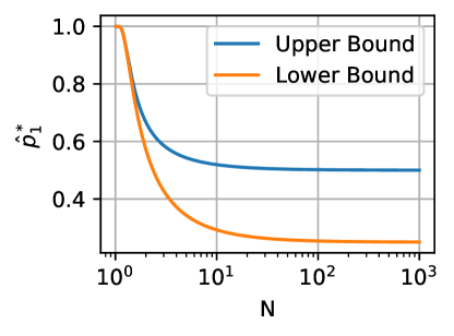
Figure 7: Plot of the upper bound (Equation 13) and the lower bound (Equation 18). We plot the upper bound (blue) and lower bound (orange) for $p_{1}=\frac{1}{2}$, $p_{2}=\frac{1}{4}$, $\epsilon=\frac{1}{4}$ and $k=2$. Both the upper bound and the lower decrease monotonically in $N$ and they both tends to $1$ as $N\to 1^{+}$.

This upper bound is monotonically decreasing in $N$ (Figure 7), implying that at large $N$, an optimal policy for pass@N must limit its max confidence to be low, thereby favoring exploration and discouraging exploitation. Furthermore, we prove:

Lemma 4.3 (Lower bound on max confidence).

Assume top two accuracies $p_{1}>p_{2}$. Then optimal policies maximizing pass@N coverage in Equation 2, subject to above accuracy and calibration constraints, must have max confidence obeying

$$\hat{p}_{1}^{*}\geq 1-\frac{(1-p_{1}+p_{2})p_{1}^{\frac{1}{1-N}}p_{2}^{\frac{1}{N-1}}}{1-p_{1}+p_{2}+p_{1}^{\frac{1}{1-N}}p_{2}^{\frac{N}{N-1}}}.$$

This lower bound is a monotonically decreasing function of $N$ (Figure 7), implying that at small $N$, optimal policies for pass@N must have high max confidence, thereby favoring exploitation and discouraging exploration. Note in the limit $N\to 1^{+}$, the lower bound is always $1$, recovering the intuitive result that the optimal policy for pass@1 is to place 100% confidence on the highest accuracy answer.

4.3 Overconfidence prevents performance gains from scaling test-time compute

To summarize the consequences of our lemmas above, among the space of approximately well calibrated policies in which higher model confidence on an answer is correlated with higher accuracy on the answer, Lemma 4.2 suggests that at large $N$ it is beneficial to unconfidently explore by assigning low model confidence to many answers, while Lemma 4.3 suggests that at small $N$ it is beneficial to confidently exploit by assigning high model confidence to one or a few answers. These lemmas make a prediction that could explain the empirical observation in Table 1 that pass@N test performance for large $N$ degrades over epochs when pass@1 is maximized at training time: namely, maximization of pass@1 makes the model overconfident, thereby preventing good performance on pass@N.

To test this theoretical prediction of model overconfidence, we estimated the max confidence of the model as $\hat{p}(y_{\mathrm{greedy}}|x)$ where $y_{\mathrm{greedy}}$ is the greedy completion to $x$ obtained by sampling autoregressively from the model $\hat{p}$, and at each step selecting the token with the highest probability. $\hat{p}(y_{\mathrm{greedy}}|x)$ approximates the max confidence $\hat{p}_{1}$ in Lemmas 4.2 and 4.3. For the model fine-tuned on MATH with CE loss, we plot the distribution of $\hat{p}(y_{\mathrm{greedy}}|x)$ over the test set in Figure 1 (leftmost). This demonstrates the model becomes progressively more confident about its greedy completion over training, thereby confirming our theoretical prediction. In Figure 1 (left) we see why this is a problem: only some of the model’s highly confident answers are correct. Thus the model becomes overconfident and largely wrong. Scaling test-time compute cannot easily rescue such a model, as over multiple samples, it is likely to confidently provide the same wrong answers, explaining the origins of poor pass@N test performance.

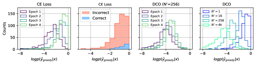
Figure 1: A model trained with CE loss becomes overconfident in its greedy completions, which harms its pass@N coverage; our proposed DCO objective limits this overconfidence. We fine-tune a Llama-3-8B base model on the MATH dataset to produce direct answers without a reasoning trace. $\hat{y}_{\text{greedy}}$ is the model’s greedy completion when sampling autoregressively and choosing the most likely token at each step. Leftmost: The model trained with CE loss assigns progressively larger confidences $\hat{p}(\hat{y}_{\text{greedy}}|x)$ to its greedy completions over the course of training. Left: At the end of the training, only a small portion of the model’s highly confident completions are correct. This will harm the model’s pass@N performance when scaling up $N$. Right: Same as leftmost but shown for the DCO loss with $N=256$. Relative to the CE loss, the model trained on DCO shows a much milder overconfidence effect. Rightmost: The confidence distribution of the greedy completions after four epochs with DCO for various choices of $N$. As $N$ increases, the model’s confidence on the greedy completion is more stringently limited, directly as a consequence of the overconfidence regularizer $F$.

5 Direct Coverage Optimization

5.1 A solution that naturally prevents overconfidence

The misalignment between CE training loss and pass@N coverage suggests a simple solution: directly optimize pass@N coverage for each training example at training time, whenever the pass@N strategy is to be used at test-time. We thus propose the Direct Coverage Optimization (DCO) objective, $\mathcal{L}_{\text{DCO}}^{N}=\mathop{\mathbb{E}}_{(x,y)\sim\mathcal{D}}\ell^{N}_{\text{DCO}}(x,y)$, where

$$\ell^{N}_{\text{DCO}}(x,y)=-\log\left(1-(1-\hat{p}(y|x))^{N}\right),$$ (3)

is the $-\log$ probability that the model produces $y$ at least once in $N$ samples given $x$. Thus for each prompt $x$ and correct completion $y$ in the training set, we maximize the probability $y$ is found in $N$ passes. This loss naturally prevents model overconfidence, as can be seen via its gradient

$$\nabla_{\theta}\ell_{\text{DCO}}^{N}(x,y)=F\left(N,\hat{p}(y|x)\right)\nabla_{\theta}\ell_{\text{CE}}(x,y)$$ (4)

where $\ell_{\mathrm{CE}}$ is the standard CE loss on a single example, and $F(N,\hat{p}(y|x))=\frac{N(1-\hat{p}(y|x))^{N-1}\hat{p}(y|x)}{1-(1-\hat{p}(y|x))^{N}}$ is an extra overconfidence regularization factor that multiplies the standard CE gradient. Note that $F(N,\hat{p}(y|x))=1$ for $N=1$, so DCO reduces to CE for pass@1. Furthermore $F(N,\hat{p}(y|x))$ monotonically decreases in the model confidence $\hat{p}(y|x)$ (see Figure 2). Thus gradients for examples $(x,y)$ on which the model is more confident are attenuated, and this attenuation is stronger for larger $N$. This justifies the interpretation of $F(N,\hat{p}(y|x))$ as a regularizer that prevents model overconfidence. Indeed, for large $N$, $F(N,\hat{p}(y|x))\approx 0$ for confidence $\hat{p}(y|x)\gtrsim 1/N$. As soon as model confidence on an example exceeds $1/N$, its gradient becomes negligible. Thus interestingly, aligning training and test better through DCO naturally yields a simple emergent regularization of model overconfidence, which was itself identified as an impediment to performance gains through scaling test-time compute in Figure 1 (leftmost).

We note in practice, the introduction of $F$ can lead to some samples in a batch contributing minimally to the current gradient step, thereby reducing the effective batch size. To maintain a stable effective batch size, we introduce a threshold $\epsilon$, and if for a given example, $(x,y)$, $F(N,\hat{p}(y|x))<\epsilon$, we replace the example with a new one.

Figure 2: The DCO objective limits overconfidence by attenuating gradients for examples on which the model is highly confident. We plot the confidence regularization factor $F(N,\hat{p}(y|x))$ in Equation 4 which attenuates CE loss gradients to obtain DCO loss gradients. $N=1$ corresponds to CE loss, where $F=1$ regardless of $\hat{p}(y|x)$. For any $N>1$, the attenuation is stronger ($F$ is smaller) for examples with higher model confidence $\hat{p}(y|x)$, and this attentuation effect increases with $N$. $F$ drops to near zero as soon as confidence $\hat{p}(y|x)$ increases to $1/N$. Thus as soon as an example’s confidence rises to $O(1/N)$ over training time, its gradient under the DCO loss cannot make the confidence rise any further. Thus DCO naturally limits overconfidence.

5.2 DCO can prevent overconfidence and rescue test-time scaling

We next test whether DCO can rescue test-time scaling by preventing model overconfidence. We first perform experiments on the MATH dataset in this section, and then in the next section we perform experiments on the LeanDojo automated theorem proving benchmark (Yang et al., 2023).

We fine-tune the LLama-3-8B-base model for 4 epochs on the MATH training set using DCO for $N=256$ and confirm that the model is far less confident on its greedy completion than when trained with CE loss after multiple training epochs (compare Figure 1 right and Figure 1 leftmost). Moreover, training with DCO at larger $N$ yields lower model greedy confidences at the end of training (Figure 1 rightmost), consistent with Lemma 4.2.

We next assess pass@N test performance as a function of $N$ for a variety of models trained by minimizing $\mathcal{L}_{\text{DCO}}^{N^{\prime}}$ for different values of $N^{\prime}$ (Figure 3). For any given $N$ in pass@N, there is an optimal $N^{\prime}$ for the training loss $\mathcal{L}_{\text{DCO}}^{N^{\prime}}$ that maximizes pass@N test coverage, yielding a Pareto optimal performance frontier (black curve) that is achieved when $N^{\prime}$ is close to $N$. In particular the model trained with CE loss (equivalent to pass@1 maximization at training) performs poorly relative to the Pareto frontier at large N when the pass@N strategy is used at test time (red curve below black at large $N$). Conversely, models trained with DCO at large $N^{\prime}$ perform poorly relative to the Pareto frontier when the pass@N strategy is used at test time with small $N$ (green curves below black at small $N$).

Together these results indicate that the alignment of the training loss $\mathcal{L}_{\text{DCO}}^{N^{\prime}}$ with the test time strategy pass@N, with $N^{\prime}$ close to $N$, is crucial for obtaining Pareto optimal performance. Moreover, these results once again confirm the tradeoff between exploration and exploitation, with good performance using pass@N test-time strategies requiring high (low) exploration with low (high) confidence at large (small) $N$. Indeed, this tradeoff prevents achieving Pareto optimality using pass@N at test-time for all $N$ via training with DCO at any single value of $N^{\prime}$.

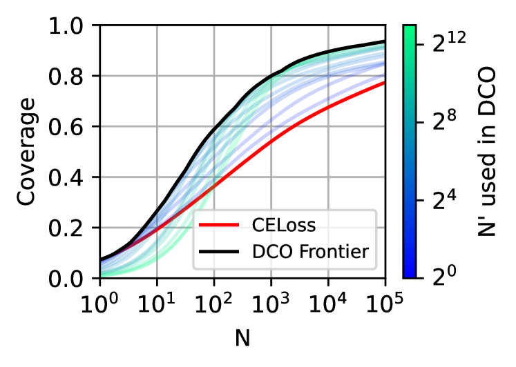
Figure 3: DCO improves on CE for pass@N test coverage over a broad range of N and traces a Pareto-optimal frontier. We fine-tune Llama-3-8B base models on the MATH dataset to produce direct answers. We fine-tune for 4 epochs one model using CE loss and several models under the $\mathcal{L}_{\text{DCO}}^{N^{\prime}}$ objective, for choices of $N^{\prime}$ indicated by color. We plot pass@N test coverage as a function of $N$, with each curve (solid red or faint blue-green) corresponding to one fine-tuned model. Note that there is no choice of $N^{\prime}$ that is optimal across all $N$ (different colors are higher at different $N$). The black curve is a Pareto-optimal performance frontier traced by the max of coverage curves for DCO over all $N^{\prime}$. Pareto-optimality at a given test strategy pass@N for some $N$ on the x-axis is obtained by DCO training for some $N^{\prime}$ close to $N$.

5.3 Improved theorem proving via ensembled tree search through a modified step-wise DCO

To further test our method in realistic settings with a verifier, we conduct experiments in theorem proving using an interactive proof assistant on the LeanDojo benchmark (Yang et al., 2023) extracted from the math library of LEAN4 (mathlib Community, 2020). In this task, at each step $i$ of the proof, the model is prompted with the current proof state $x[i]$, and it outputs a proof tactic $y[i]$ with a trainable model probability $\hat{p}(y[i]|x[i])$. The proof assistant takes the sampled tactic $y[i]$, verifies whether it is a valid tactic, and if so, returns the next proof state $x[i+1]$ after the tactic $y[i]$ is applied. The model then samples the next tactic $y[i+1]$. At test time this interactive process between the model and the assistant continues until either: (1) it terminates in an invalid tactic; (2) hits a maximal allowed search depth set by computational constraints; or (3) terminates in a successful proof of the initial proof goal as verified by the proof assistant.

In our experiments, we use LEAN4 (Moura & Ullrich, 2021) as the formal proof language. We start from the model Qwen2.5-Math-1.5B (Yang et al., 2024), and fine-tune it on the LeanDojo benchmark (Yang et al., 2023). In contrast to solving math problems above where the model first autoregressively generates an entire answer $y$ according to $\hat{p}(y|x)$ and then the entire $y$ is verified for correctness, in theorem proving we must obtain correct tactics $y[i]$, as verified by the proof assistant, at every proof step $i$. A straightforward application of DCO fine-tuning in this setting then involves replacing the model confidence $\hat{p}(y|x)$ in  Equation 3 on a single math answer $y$, with the model confidence on an entire successful, complete $k$ step proof $\hat{p}(y[0],...,y[k-1]|x[0])=\prod_{i=0}^{k-1}\hat{p}(y[i]|x[i])$. Because of the chain rule, the DCO gradient on a single proof has the same form as in Equation 4 but with $F(N,\hat{p}(y|x))$ replaced with $F(N,\prod_{i=0}^{k-1}\hat{p}\left(y[i]|x[i]\right))$.

We naively applied this DCO fine-tuning method with $N=4$k and we evaluated the resulting model, as well as a baseline model trained with CE loss, on MiniF2F. As a test strategy, we used pass@4k. The baseline model fine-tuned with CE loss achieves a proof success rate of 37.4%, while model fine-tuned with DCO at $N=4$k achieves a 38.7% success rate. Thus, a naive application of DCO to theorem proving by matching the parameter $N$ in DCO to the parameter $N$ in pass@N achieves only a modest improvement.

However, in theorem proving, since every single intermediate proof step tactic $y[i]$ must be valid, it is natural to consider a step-wise generalization of DCO. For example, at each step $i$, the model chooses a tactic $y[i]$ with confidence $\hat{p}(y[i]|x[i])$. Our proposed step-wise DCO optimizes this single-step confidence according to Equation 4 as before, except now the step-wise confidence regularizer is given by $F(N_{\text{eff}},\hat{p}(y[i]|x[i]))$. Here one can think of $N_{\text{eff}}$ as a step-wise DCO hyperparameter that controls the exploration width at every proof step. In essence, the confidence regularizer prevents the confidence of any chosen tactic from becoming much higher than $1/N_{\text{eff}}$. Since the sum of the confidences over all tactics at each step must be $1$, this means that at test time, model exploration at each step corresponds to searching on a search tree in which each proof state $x[i]$ allows the exploration of approximately only $N_{\text{eff}}$ tactics. Thus using $N_{\text{eff}}$ in step-wise DCO during fine-tuning selects the approximate branching factor $N_{\text{eff}}$ of the model’s proof search tree at test time (see  Figure 4).

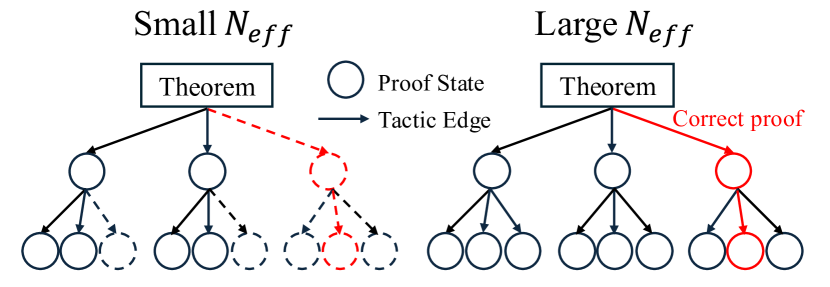
Figure 4: Inverse confidence $N_{\text{eff}}$ at training time controls search-tree exploration shapes at test-time. We show, qualitatively, two proof search trees (solid lines) obtained when training at small $N_{\mathrm{eff}}$ (left) and large $N_{\mathrm{eff}}$ (right). Both trees start from the same theorem statement (top), circles denote proof states, directed edges denote tactics, solid edges are assigned non-negligible model confidence and are explored, while dashed edges are not. Small $N_{\mathrm{eff}}$ leads to a small branching factor (left), which can fail if the correct proof (red path) is not in the narrow search tree. Larger $N_{\mathrm{eff}}$ expands the search tree to include the correct proof (right). However, if $N_{\mathrm{eff}}$ is too large ($N_{\mathrm{eff}}^{k}\gg N$ for a theorem with $k$ proof steps), the sampling probability of the correct proof will decrease as $N_{\mathrm{eff}}^{-k}$ and the pass@N coverage $\mathcal{C}^{N}\approx N/N_{\mathrm{eff}}^{k}$ decreases as $N_{\mathrm{eff}}$ increases. In essence the correct proof is too hard to find in a search tree that is too wide. Overall, we see that inverse confidence $N_{\mathrm{eff}}$ chosen at training time constitutes a simple but powerful knob to control a tradeoff between exploitation and exploration on proof search trees of varying shapes at test time.

In particular, a valid (partial) proof of length $k$ will have probability of order $N_{\text{eff}}^{-k}$. Thus small $N_{\text{eff}}$ limits the exploration at test time to a tree with small branching factor, but allows longer proofs with larger numbers of steps $k$ to have higher sampling probability. This limited width search strategy should work well at test time using pass@N as long as two conditions hold: (1) a successful proof of length $k$ is present in the search tree of branching factor $N_{\text{eff}}$; and (2) the $N$ in pass@N at test time is large enough that this proof of probability $O(N_{\text{eff}}^{-k})$ is selected with high probability in $N$ passes (which starts to occur as soon as $N\gtrsim N_{\text{eff}}^{k}$).

Conversely, larger $N_{\text{eff}}$ allows for more exploration at test time using a wider search tree of larger branching factor, but it makes finding longer proofs with large $k$ harder, since the approximate success condition for pass@N of $N>N_{\text{eff}}^{k}$ is harder to satisfy at fixed $N$ and large $N_{\text{eff}}$ and $k$. However, this wide exploration strategy can work well for short proofs with small $k$ if a successful short proof does not lie in the limited width search tree obtained at small $N_{\text{eff}}$, but does lie in a wider search tree at larger $N_{\text{eff}}$ (Figure 4, right).

We note that the mean and median lengths of the proofs in the training set is 4.2 and 2 respectively. Thus we explore fine-tuning on LeanDojo with the step-wise DCO algorithm DCO^step with $N_{\text{eff}}$ ranging from $1$ (corresponding to standard CE-loss training) to $N_{\text{eff}}=32$. We evaluated the pass@N test performance for $N=4$k of each of the resulting models on Mathlib and MiniF2F test sets, finding improved performance at larger $N_{\text{eff}}$ compared to the baseline $N_{\text{eff}}=1$ CE loss training (Table 2). Interestingly, we find that the optimal $N_{\text{eff}}$ increases with more passes at test time (Table 4), similar to the Pareto frontier in Figure 3.

Since different choices of $N_{\text{eff}}$ correspond to very different search strategies at test time, specializing in finding short proofs on wide search trees for large $N_{\text{eff}}$ and long proofs on narrow search trees for small $N_{\text{eff}}$, we hypothesized that ensembling these methods could significantly boost performance. We found this was indeed the case (ensemble entry in Table 2). Of course the Ensemble strategy samples $5\times 4$k times, so a proper baseline is CE loss with the same test-time compute of pass@N with $N=20$k. We obtained the proof success rate for this baseline to be 57.0% on Mathlib and 39.5% on MiniF2F. The ensemble strategy outperforms this stringent baseline with significant excesses of $5.2\%$ on Mathlib and $4.1\%$ on MiniF2F.

Overall, these results indicate that varying $N_{\text{eff}}$ in step-wise DCO at training time allows a diversity of tree search strategies trading depth and breadth that can be effectively exploited by simply scaling test time compute via pass@N.

Table 2: Proof success rate using pass@4k at test time on Mathlib and MiniF2F and training with DCO^step for different $N_{\text{eff}}$.

	Mathlib	MiniF2F
$N_{\mathrm{eff}}=1$ (CE loss)	55.6%	37.4%
$N_{\mathrm{eff}}=4$	56.4%	39.0%
$N_{\mathrm{eff}}=8$	56.1%	39.5%
$N_{\mathrm{eff}}=16$	56.5%	37.0%
$N_{\mathrm{eff}}=32$	55.8%	37.4%
Ensemble of above $N_{\mathrm{eff}}$	62.2%	43.6%
$N_{\mathrm{eff}}=1$ (5x test compute)	57.0%	39.5%

5.4 Approximate DCO also improves MATH answering with chain-of-thought reasoning

In Section 5.2 on solving problems in MATH, the model is trained to directly give an answer $y$ to a problem $x$. In this case, one can implement DCO at training time by explicitly computing the model confidence $\hat{p}(y|x)$ and using it in Equation 4. However, in an alternate powerful Chain-of-Thought (CoT) training paradigm, the training data consists of triplets $(x,c,y)$ where $x$ and $y$ are the problem and answer as before, but now $c$ is a CoT reasoning trace that explains how to derive $y$ from $x$. The model is trained on the triplet $(x,c,y)$, and at test time, when given a new problem $x^{\prime}$, it generates a reasoning trace $c^{\prime}$ and answer $y^{\prime}$. Importantly, the model is evaluated on whether its answer $y^{\prime}$ is correct independent of the reasoning trace $c^{\prime}$ it emits.

Thus, to estimate the probability $\hat{p}(y|x)$ that the model assigns to any answer $y$, one can no longer compute it directly as in the direct answer case in Section 5.2. Instead, one must marginalize over all possible reasoning traces $c$ to obtain $\hat{p}(y|x)=\sum_{c}\hat{p}(y,c|x)$. Because exact marginalization is intractable, to employ DCO in Equation 4 in the CoT setting, we replace the marginalization with a Monte Carlo estimate of $\hat{p}(y|x)$, and insert this estimate into the overconfidence regularization factor $F$ in Equation 4. We call this algorithm approximate DCO, denoted by DCO^a. We also compute Monte Carlo estimates of the probability the model assigns to its most likely final answer, $\hat{p}(y^{\mathrm{mode}}|x)$, as a proxy for the greedy completion probability $\hat{p}(y^{\mathrm{greedy}}|x)$ used to study overconfidence in the direct answer setting in  Section 5.2. Note that in the CoT setting the greedy answer would correspond to a single most likely reasoning trace, but we want the probability of the most likely final answer obtained by marginalizing over all reasoning traces.

We conduct experiments on the MATH dataset. For the baseline experiment, we first fine-tune a Llama-3-8B-base model with CE loss on the golden CoT solutions. We find in Table 3 that pass@1 coverage robustly improves over the course of CE loss training. Intriguingly, in the CoT setting, overfitting induced by the misalignment of CE loss at training time with the pass@N strategy at test time, is not as severe as in the direct answer setting in Table 1. If overfitting indeed arises from the model overconfidence induced by CE loss, we would expect that minimizing CE loss in the CoT setting does not make the model as overconfident as it does in the direct answer case. This is indeed confirmed: compare Figure 5 left, in the CoT case, where the confidence of the modal answer shifts slightly to the right over epochs, to Figure 1 leftmost, in the direct answer case, where it shifts much further right.

We next explore the properties of DCO^a with $N=64$. We find that training with DCO^a ($N^{\prime}=64$) underperforms relative to training with CE loss for pass@1 at test time, but outperforms when the test strategy is pass@N for larger $N$ (Table 3). This is similar to the direct answer behavior in Figure 3. The largest improvement occurs when training with DCO^a at $N^{\prime}=64$ is aligned with pass@N at $N=64$. Furthermore, our theory in Section 4.2 predicts that DCO^a training should lower model confidence relative to CE loss training, thereby explaining the improved pass@64 performance. We confirm this prediction in Figure 5 right, which reveals that DCO^a successfully prevents the model from becoming overconfident in its most likely answer $y^{\mathrm{mode}}$.

Overall these results once again validate our theory and algorithmic approaches, now in a CoT reasoning setting. In essence, improved performance by scaling test time compute via a pass@N strategy at large $N$ can be best obtained by aligning the training strategy via choosing DCO^a with the same $N$, and the origin of the performance improvement comes from limiting model overconfidence.

Table 3: Pass@N test coverage on MATH obtained from fine-tuning Llama-3-8B-base on CoT traces using CE or DCO^a loss with $N=64$. $\pm$ error is standard error of the mean.

		pass@1	pass@16	pass@64
Epoch 1	CE	4.3 $\pm$ 0.1%	30.2 $\pm$ 0.7%	51.2 $\pm$ 1.2%
	DCOa	5.0 $\pm$ 0.1%	34.2 $\pm$ 0.6%	55.3 $\pm$ 1.0%
Epoch 3	CE	9.0 $\pm$ 0.1%	41.6 $\pm$ 0.4%	61.7 $\pm$ 0.4%
	DCOa	8.3 $\pm$ 0.1%	42.6 $\pm$ 0.6%	63.1 $\pm$ 0.8%
Epoch 5	CE	9.9 $\pm$ 0.1%	40.9 $\pm$ 0.4%	60.9 $\pm$ 0.6%
	DCOa	7.8 $\pm$ 0.1%	42.8 $\pm$ 0.5%	64.3 $\pm$ 0.6%

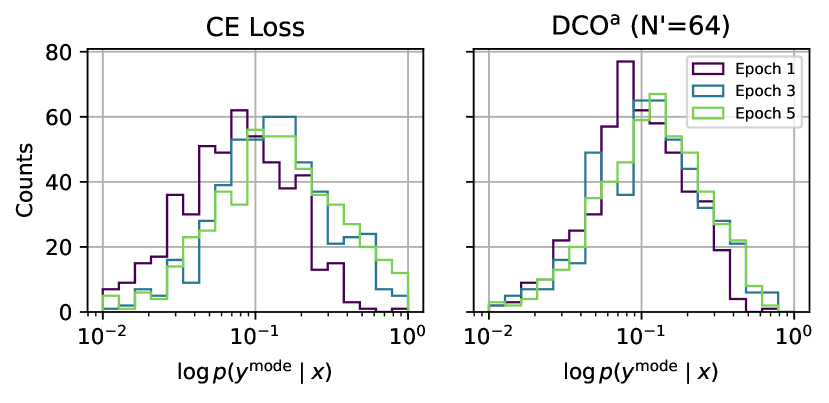
Figure 5: Overconfidence persists in CoT fine-tuning with CE loss, which DCO^a successfully limits. We fine-tune a Llama-3-8B base model on the MATH dataset on CoT traces. We plot the distribution of the estimated model confidences $\hat{p}(y^{\mathrm{mode}}|x)$ over samples in the test set at various points in training. Left: for CE loss, the model becomes more confident in its most likely answers, as the confidence distribution shifts slightly to the right as training progresses. This effect is milder than in the direct answer setting (Figure 1). Right: for DCO^a loss, the rightward shift in the confidence distribution of the most likely answer over training time is limited; DCO^a again limits overconfidence relative to CE loss.

6 Discussion

In summary, all our results suggest the need for a tight co-design of two traditionally separate phases of LLM development: (1) model training or fine-tuning and (2) test-time search/reasoning strategies and budget. If the former is misaligned with the latter, then more training can actually impair performance gains from scaling test-time compute. But if they are properly co-designed, end-to-end training and test time performance can be far more effective. We have shown how to modify standard cross-entropy loss for training to be better aligned to a pass@N strategy for large N at testing. Moreover, we have suggested and empirically confirmed why this co-design of training loss and pass@N strategy is essential, because optimal policies for pass@N at large N should unconfidently explore while the optimal policies for pass@N at small N should confidently exploit.

This notion of co-design opens up many more theoretical and empirical questions associated with different test-time strategies such as self-verification and MCTS. Furthermore, one can go beyond test-time search to recursive self-improvement, where new solutions found by search are filtered and then used to retrain the model. A theoretical understanding of the capabilities achievable by recursive self-improvement through co-design of training, search, and filtering, remains an outstanding research problem.

Appendix A Proofs

A.1 Proof of approximately well calibration under optimal policy

Lemma A.1.

Given any problem, let $\hat{p}_{i}$ denote the model probability or confidence assigned to answer $i$, and assume answers are sorted from highest to lowest confidence so that $\hat{p}_{i}\geq\hat{p}_{i+1},\forall\,i\geq 1$. Let $p_{i}$ be the probability that answer $i$ is actually correct across all the problems. Then optimal policies maximizing pass@N coverage in Equation 2 (denoted by $\hat{p}_{i}^{*}$) is approximately well calibrated, i. e. higher confidence implies higher or equal probability of being correct, i.e. $p_{i}\geq p_{i+1},\forall\,i\geq 1$.

Proof.

Let $R$ be the total number of answers the model can generate. Here $R$ could possibly equal infinity. Let $\hat{p}_{i}^{*}$ denote the model probability or confidence assigned to answer $i$ under optimal policy maximizing pass@N coverage in Equation 2. Let $A_{i}$ be the event that the $i$^th ranked answer is not chosen in the $N$ passes and $B_{i}$ be the event that $i$^th ranked answer is chosen in the $N$ passes. Let $1_{B_{i}}$ be the indicator function of $B_{i}$. Then, given an event $\omega$, the probability of getting the correct answer is $\sum_{i=1}^{R}p_{i}1_{B_{i}}(\omega)$. Hence, the expected probability of getting the correct answer is

$$\mathbb{E}\left(\sum_{i=1}^{R}p_{i}1_{B_{i}}\right)=\sum_{i=1}^{R}p_{i}\mathbb{P}(B_{i})=\sum_{i=1}^{R}p_{i}(1-\mathbb{P}(A_{i}))=1-\sum_{i=1}^{R}p_{i}\mathbb{P}(A_{i})=1-\sum_{i=1}^{R}p_{i}(1-\hat{p}_{i}^{*})^{N},$$ (5)

If the current strategy is already optimal, any small change of $(\hat{p}_{1}^{*},...,\hat{p}_{R}^{*})$ would not increase the expected probability of getting the correct answer. Now suppose we don’t always have $p_{i}\geq p_{i+1}$, in other words, $p_{j}<p_{j+1}$ for some $j\geq 1$. If $\hat{p}_{j}^{*}<\hat{p}_{j+1}^{*}$, we have

$$\mathbb{E}\left(\sum_{i=1}^{R}p_{i}1_{B_{i}}\right)<1-\sum_{i=1}^{j-1}p_{i}(1-\hat{p}_{i}^{*})^{N}-\sum_{i=j+1}^{R}p_{i}(1-\hat{p}_{i}^{*})^{N}-p_{j+1}(1-\hat{p}_{j}^{*})^{N}-p_{j}(1-\hat{p}_{j+1}^{*})^{N},$$ (6)

where the last inequality says that we can increase the expected probability of getting the correct answer by swapping the confidence on answer originally labeled as $j$ and $j+1$, which is a contradiction. If $\hat{p}_{j}^{*}=\hat{p}_{j+1}^{*}$, then for all $\delta>0$ sufficiently small, we always have

$$\mathbb{E}\left(\sum_{i=1}^{R}p_{i}1_{B_{i}}\right)<1-\sum_{i=1}^{j-1}p_{i}(1-\hat{p}_{i}^{*})^{N}-\sum_{i=j+1}^{R}p_{i}(1-\hat{p}_{i}^{*})^{N}-p_{j}(1-\hat{p}_{j}^{*}-\delta)^{N}-p_{j+1}(1-\hat{p}_{j+1}^{*}+\delta)^{N},$$ (7)

which also contradict with the current policy being optimal. ∎

A.2 Proof of Lemma 4.2

Proof.

Let $R$ be the total number of answers the model can generate. Here $R$ could possibly equal infinity. Let $\hat{p}_{i}^{*}$ denote the model probability or confidence assigned to answer $i$ under optimal policy maximizing pass@N coverage in Equation 2. Let $A_{i}$ be the event that the $i$^th ranked answer is not chosen in the $N$ passes and $B_{i}$ be the event that $i$^th ranked answer is chosen in the $N$ passes. Let $1_{B_{i}}$ be the indicator function of $B_{i}$. Then, given an event $\omega$, the probability of getting the correct answer is $\sum_{i=1}^{R}p_{i}1_{B_{i}}(\omega)$. Hence, the expected probability of getting the correct answer is

$$\mathbb{E}\left(\sum_{i=1}^{R}p_{i}1_{B_{i}}\right)=\sum_{i=1}^{R}p_{i}\mathbb{P}(B_{i})=\sum_{i=1}^{R}p_{i}(1-\mathbb{P}(A_{i}))=1-\sum_{i=1}^{R}p_{i}\mathbb{P}(A_{i})=1-\sum_{i=1}^{R}p_{i}(1-\hat{p}_{i})^{N}$$ (8)

Optimal strategy maximizes Equation 8. Let $\pi_{1}(\{\hat{p}_{1}^{*},...,\hat{p}_{m}^{*}\})\equiv\hat{p}_{1}^{*}$ be the projection onto the first entry, then

$$\hat{p}_{1}^{*}=\pi_{1}\left(\underset{\{\hat{p}_{i}\}_{i=1}^{R}}{\text{argmin}}\{\sum_{i=1}^{R}p_{i}(1-\hat{p}_{i})^{N}\}\right).$$ (9)

The proof is then motivated by the following intuition: given the constraint $\sum_{i=1}^{k}p_{i}\geq 1-\epsilon$, $\hat{p}_{1}^{*}$ attains its largest possible value when the $p_{j}\;(j\geq 2)$ are as small as possible. It is worth noting that first

$$\pi_{1}\left(\underset{\{\hat{p}_{i}\}_{i=1}^{R}}{\text{argmin}}\{\sum_{i=1}^{R}p_{i}(1-\hat{p}_{i})^{N}\}\right)\leq\pi_{1}\left(\underset{\{\hat{p}_{i}\}_{i=1}^{k}}{\text{argmin}}\{\sum_{i=1}^{k}p_{i}(1-\hat{p}_{i})^{N}+\sum_{i=k+1}^{R}p_{i}\}\right).$$ (10)

Second, given $p_{1}$ and $\sum_{i=1}^{k}p_{i}\geq 1-\epsilon$, we have

$$\pi_{1}\left(\underset{\{\hat{p}_{i}\}_{i=1}^{k}}{\text{argmin}}\{\sum_{i=1}^{k}p_{i}(1-\hat{p}_{i})^{N}+\sum_{i=k+1}^{R}p_{i}\}\right)\leq\pi_{1}\left(\underset{\{\hat{p}_{i}\}_{i=1}^{k}}{\text{argmin}}\{p_{1}(1-\hat{p}_{1})^{N}+\sum_{i=2}^{k}\frac{1-p_{1}-\epsilon}{k-1}(1-\hat{p}_{i})^{N}+\sum_{i=k+1}^{R}p_{i}\}\right).$$ (11)

Third, fix $\hat{p}_{1}$, Jensen’s inequality tells us that

$$p_{1}(1-\hat{p}_{1})^{N}+\sum_{i=2}^{k}\frac{1-p_{1}-\epsilon}{k-1}(1-\hat{p}_{i})^{N}\geq p_{1}(1-\hat{p}_{1})^{N}+(1-p_{1}-\epsilon)(1-\frac{1-\hat{p}_{1}}{k-1})^{N}.$$ (12)

Combining all three inequalities above we have

$$\hat{p}_{1}^{*}=\pi_{1}\left(\underset{\{\hat{p}_{i}\}_{i=1}^{k}}{\text{argmin}}\{\sum_{i=1}^{R}p_{i}(1-\hat{p}_{i})^{N}\}\right)\leq\underset{\hat{p}_{1}}{\text{argmin}}\{p_{1}(1-\hat{p}_{1})^{N}+(1-p_{1}-\epsilon)(1-\frac{1-\hat{p}_{1}}{k-1})^{N}\}.$$ (13)

The right hand side of Equation 13 can be computed by taking derivatives, and we arrive at

$$\hat{p}_{1}^{*}\leq\underset{\hat{p}_{1}}{\text{argmin}}\{p_{1}(1-\hat{p}_{1})^{N}+(1-p_{1}-\epsilon)(1-\frac{1-\hat{p}_{1}}{k-1})^{N}\}=1-\frac{k-1}{(k-1)^{\frac{N}{N-1}}p_{1}^{\frac{1}{N-1}}\left(1-p_{1}-\epsilon\right){}^{\frac{1}{1-N}}+1}.$$ (14)

∎

A.3 Proof of Lemma 4.3

Proof.

The following proof is motivated by the following intuition: given the values of $p_{1}$ and $p_{2}$, $\hat{p}_{1}^{*}$ attains its smallest possible value when the $p_{j}\;(j\geq 3)$ are as large as possible. Let $s$ be the smallest integer such that $p_{1}+sp_{2}\geq 1$. We have,

$$\hat{p}_{1}^{*}=\pi_{1}\left(\underset{\{\hat{p}_{i}\}_{i=1}^{R}}{\text{argmin}}\{\sum_{i=1}^{R}p_{i}(1-\hat{p}_{i})^{N}\}\right)\geq\pi_{1}\left(\underset{\{\hat{p}_{i}\}_{i=1}^{s+1}}{\text{argmin}}\{p_{1}(1-\hat{p}_{1})^{N}+\sum_{i=2}^{s+1}p_{2}(1-\hat{p}_{i})^{N}\}\right).$$ (15)

Second, for a fixed $\hat{p}_{1}$, Jensen’s inequality tells us that

$$p_{1}(1-\hat{p}_{1})^{N}+\sum_{i=2}^{s+1}p_{2}(1-\hat{p}_{i})^{N}\geq p_{1}(1-\hat{p}_{1})^{N}+sp_{2}(1-\frac{1-\hat{p}_{1}}{s})^{N}$$ (16)

Therefore, we have

$$\pi_{1}\left(\underset{\{\hat{p}_{i}\}_{i=1}^{s+1}}{\text{argmin}}\{p_{1}(1-\hat{p}_{1})^{N}+\sum_{i=2}^{s+1}p_{2}(1-\hat{p}_{i})^{N}\}\right)=\underset{\hat{p}_{1}}{\text{argmin}}\{p_{1}(1-\hat{p}_{1})^{N}+sp_{2}(1-\frac{1-\hat{p}_{1}}{s})^{N}\}$$ (17)

Computing the right hand side of Equation 17 by taking derivatives we have

$$\hat{p}_{1}^{*}\geq\underset{\hat{p}_{1}}{\text{argmin}}\{p_{1}(1-\hat{p}_{1})^{N}+sp_{2}(1-\frac{1-\hat{p}_{1}}{s})^{N}\}=1-\frac{sp_{1}^{\frac{1}{1-N}}p_{2}^{\frac{1}{N-1}}}{s+p_{1}^{\frac{1}{1-N}}p_{2}^{\frac{1}{N-1}}}.$$ (18)

Since $s$ is the smallest integer such that $p_{1}+sp_{2}\geq 1$, we have

$$1+p_{2}>p_{1}+sp_{2},$$ (19)

Combining Equation 19 and Equation 18 we arrive at

$$\hat{p}_{1}^{*}\geq 1-\frac{(1-p_{1}+p_{2})p_{1}^{\frac{1}{1-N}}p_{2}^{\frac{1}{N-1}}}{1-p_{1}+p_{2}+p_{1}^{\frac{1}{1-N}}p_{2}^{\frac{N}{N-1}}}.$$ (20)

∎

Appendix B Experimental details

All experiments are performed on machines with 8 NVIDIA H100 GPUs or 8 NVIDIA A100 GPUs. Our codebase uses PyTorch (Ansel et al., 2024), Accelerate (Gugger et al., 2022), and deepspeed (https://github.com/microsoft/DeepSpeed) to enable efficient training with memory constraints, and vllm (Kwon et al., 2023) for efficient inference. Code will be made available here.

MATH. For experiments with MATH dataset, we fine-tune the Llama-3-8B-base (Grattafiori et al., 2024) on the MATH (Hendrycks et al., 2021) dataset. We start from the base model rather than Llama-3-8B-Instruct to avoid potential leakage of the MATH dataset into Llama-3-8B-Instruct through post-training process. We follow Lightman et al. (2024) and use $12,000$ problems for training and the remaining $500$ for testing. In Sections 4 and 5.2 and Figures 1 and 3, we fine-tune the model for 4 epochs with a learning rate of 2e-5 and batch size 64. We adopt a linear learning rate warmup in the first 20 steps. For experiments with DCO, some of the data may have an extreme confidence regularizer value, if the model is already quite confident in answers to certain problems. To maintain an approximately fixed batch size, we set a threshold of $0.3$ on the confidence regularizer $F$. Any training data examples with an $F$ lower than this threshold will be replaced with new training examples to construct the batch. For the CoT experiments in Section 5.4, we use learning rate 2e-5 and batch size 128, with the same learning rate warmup.

Theorem proving. We adopt the random train and test split as introduced in Yang et al. (2023). The random test set includes 2,000 theorems. We fine-tune the model Qwen2.5-Math-1.5B (Yang et al., 2024) on the training set for 3 epochs with learning rate 1e-5 and batch size 64. We adopt a linear learning rate warmup in the first 20 steps. To evaluate the model, we use LeanDojo (Yang et al., 2023) to interact with the proof assistant. We impose a maximum wall clock time for each theorem, in addition to limiting the number of passes per problem. For experiments with 4k passes, the time budget is fixed at 5,000 seconds. In order to avoid the model going infinitely deep in the search tree, we limit the number of proof steps to be at most 50.

DCO^a objective. The DCO^a introduced in Section 5.4 is an approximation for DCO. To construct a batch of size $B$ with DCO^a, we process batches of samples sequentially; for each batch, we run online inference on each of the samples and discard all samples with probability of success rate larger than $p^{\mathrm{thresh}}$. We choose to discard samples which have a DCO confidence reguarizer $F$ lower than 0.01, corresponding to $p^{\mathrm{thresh}}=0.1$ for $N^{\prime}=64$. This process continues until we have enough training data for a single batch. In Figure 6, we plot the number of discarded samples as a function of training step for our DCO^a experiments (same ones as in Table 3).

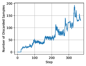
Figure 6: Number of discarded samples as a function of training step for the DCO^a experiments. The step structure reflects the model revisiting examples it has seen previously in training, where each step closely matches the start of a new epoch.

Implementing online inference. Throughout our experiments and analysis, we extensively use the open-source vllm package (Kwon et al., 2023) for efficient inference. Integrating inference into the training loop to enable training under the DCO^a objective, as in Section 5.4, poses a challenging implementation problem. We solve this problem by placing vllm worker processes, which together perform inference on all GPUs, in a separate process group and use Ray (https://github.com/ray-project/ray) to isolate them from the training loop. This enables running concurrent training and inference on the same set of GPUs. We believe this inference in the loop setup will be useful to the community, as it enables straightforward implementation of online data filtering approaches for LLM training.

Appendix C Addtional results

C.1 Theorem proving

In Table 4, we show additional results for model performance under the DCO^STEP objective. We find that the optimal $N_{\text{eff}}$ grows with increasing passes, agreeing with results in Sections 5.2 and 5.4. We also conduct expert iteration (Anthony et al., 2017; Polu et al., 2023) on Mathlib with theorems that do not have proof traces in the training set. We use pass@1k to prove those theorems. We find that our algorithm achieves a stronger improvement over the baseline for pass@4k after the 1^st iteration. This improvement might result from the fact that the models can prove more easy theorems where the model has a higher confidence. As a result, we believe our method will perform better with expert iteration.

Table 4: Success rate on lean-dojo benchmark random test set trained with DCO^step.

	Expert iteration 0					Expert iteration 1
DCOstep	pass@16	pass@64	pass@256	pass@1k	pass@4k	pass@16	pass@256	pass@4k
$N_{\mathrm{eff}}=1$ (CE)	30.0%	38.75%	46.05	50.75%	55.55%	40.3%	52.65%	58.55%
$N_{\mathrm{eff}}=4$	30.15%	39.5%	47.2%	52.95%	56.35%	40.8%	53.05%	59.45%
$N_{\mathrm{eff}}=8$	30.2%	38.9%	47.15%	52.7%	56.1%	40.1%	53.25%	59.5%
$N_{\mathrm{eff}}=16$	28.65%	46.7%	46.45%	52.9%	56.5%	39.05%	52.8%	60.05%
$N_{\mathrm{eff}}=32$	26.05%	46.7%	45.6%	51.5%	55.8%	37.05%	52.2%	59.15%
Ensemble	40.6%	49.15%	54.6%	59.0%	62.15%	49.05%	59.3%	64.8%

C.2 Plot of the upper bound and the lower bound

References

- Ansel et al. (2024) Ansel, J., Yang, E., He, H., Gimelshein, N., Jain, A., Voznesensky, M., Bao, B., Bell, P., Berard, D., Burovski, E., Chauhan, G., Chourdia, A., Constable, W., Desmaison, A., DeVito, Z., Ellison, E., Feng, W., Gong, J., Gschwind, M., Hirsh, B., Huang, S., Kalambarkar, K., Kirsch, L., Lazos, M., Lezcano, M., Liang, Y., Liang, J., Lu, Y., Luk, C., Maher, B., Pan, Y., Puhrsch, C., Reso, M., Saroufim, M., Siraichi, M. Y., Suk, H., Suo, M., Tillet, P., Wang, E., Wang, X., Wen, W., Zhang, S., Zhao, X., Zhou, K., Zou, R., Mathews, A., Chanan, G., Wu, P., and Chintala, S. PyTorch 2: Faster Machine Learning Through Dynamic Python Bytecode Transformation and Graph Compilation. In 29th ACM International Conference on Architectural Support for Programming Languages and Operating Systems, Volume 2 (ASPLOS ’24). ACM, April 2024. doi: 10.1145/3620665.3640366. URL https://pytorch.org/assets/pytorch2-2.pdf.
- Anthony et al. (2017) Anthony, T., Tian, Z., and Barber, D. Thinking fast and slow with deep learning and tree search. In Guyon, I., Luxburg, U. V., Bengio, S., Wallach, H., Fergus, R., Vishwanathan, S., and Garnett, R. (eds.), Advances in Neural Information Processing Systems, volume 30. Curran Associates, Inc., 2017. URL https://proceedings.neurips.cc/paper_files/paper/2017/file/d8e1344e27a5b08cdfd5d027d9b8d6de-Paper.pdf.
- Azerbayev et al. (2024) Azerbayev, Z., Schoelkopf, H., Paster, K., Santos, M. D., McAleer, S. M., Jiang, A. Q., Deng, J., Biderman, S., and Welleck, S. Llemma: An open language model for mathematics. In The Twelfth International Conference on Learning Representations, 2024. URL https://openreview.net/forum?id=4WnqRR915j.
- Brown et al. (2024) Brown, B., Juravsky, J., Ehrlich, R., Clark, R., Le, Q. V., Ré, C., and Mirhoseini, A. Large language monkeys: Scaling inference compute with repeated sampling, 2024. URL https://arxiv.org/abs/2407.21787.
- Chen et al. (2021) Chen, M., Tworek, J., Jun, H., Yuan, Q., de Oliveira Pinto, H. P., Kaplan, J., Edwards, H., Burda, Y., Joseph, N., Brockman, G., Ray, A., Puri, R., Krueger, G., Petrov, M., Khlaaf, H., Sastry, G., Mishkin, P., Chan, B., Gray, S., Ryder, N., Pavlov, M., Power, A., Kaiser, L., Bavarian, M., Winter, C., Tillet, P., Such, F. P., Cummings, D., Plappert, M., Chantzis, F., Barnes, E., Herbert-Voss, A., Guss, W. H., Nichol, A., Paino, A., Tezak, N., Tang, J., Babuschkin, I., Balaji, S., Jain, S., Saunders, W., Hesse, C., Carr, A. N., Leike, J., Achiam, J., Misra, V., Morikawa, E., Radford, A., Knight, M., Brundage, M., Murati, M., Mayer, K., Welinder, P., McGrew, B., Amodei, D., McCandlish, S., Sutskever, I., and Zaremba, W. Evaluating large language models trained on code, 2021. URL https://arxiv.org/abs/2107.03374.
- Chow et al. (2024) Chow, Y., Tennenholtz, G., Gur, I., Zhuang, V., Dai, B., Thiagarajan, S., Boutilier, C., Agarwal, R., Kumar, A., and Faust, A. Inference-aware fine-tuning for best-of-n sampling in large language models. arXiv preprint arXiv:2412.15287, 2024. URL https://arxiv.org/pdf/2412.15287.
- Chung et al. (2022) Chung, H. W., Hou, L., Longpre, S., Zoph, B., Tay, Y., Fedus, W., Li, Y., Wang, X., Dehghani, M., Brahma, S., Webson, A., Gu, S. S., Dai, Z., Suzgun, M., Chen, X., Chowdhery, A., Castro-Ros, A., Pellat, M., Robinson, K., Valter, D., Narang, S., Mishra, G., Yu, A., Zhao, V., Huang, Y., Dai, A., Yu, H., Petrov, S., Chi, E. H., Dean, J., Devlin, J., Roberts, A., Zhou, D., Le, Q. V., and Wei, J. Scaling instruction-finetuned language models, 2022. URL https://arxiv.org/abs/2210.11416.
- DeepSeek-AI: Daya Guo et al. (2025) DeepSeek-AI: Daya Guo, Dejian Yang, H. Z. et al. Deepseek-r1: Incentivizing reasoning capability in llms via reinforcement learning, 2025. URL https://arxiv.org/abs/2501.12948.
- Grattafiori et al. (2024) Grattafiori, A., Dubey, A., Jauhri, A., Pandey, A., et al. The llama 3 herd of models, 2024. URL https://arxiv.org/abs/2407.21783.
- Gugger et al. (2022) Gugger, S., Debut, L., Wolf, T., Schmid, P., Mueller, Z., Mangrulkar, S., Sun, M., and Bossan, B. Accelerate: Training and inference at scale made simple, efficient and adaptable. https://github.com/huggingface/accelerate, 2022.
- Hendrycks et al. (2021) Hendrycks, D., Burns, C., Kadavath, S., Arora, A., Basart, S., Tang, E., Song, D., and Steinhardt, J. Measuring mathematical problem solving with the MATH dataset. In Thirty-fifth Conference on Neural Information Processing Systems Datasets and Benchmarks Track (Round 2), 2021. URL https://openreview.net/forum?id=7Bywt2mQsCe.
- Jones (2021) Jones, A. L. Scaling scaling laws with board games, 2021. URL https://arxiv.org/abs/2104.03113.
- Kwon et al. (2023) Kwon, W., Li, Z., Zhuang, S., Sheng, Y., Zheng, L., Yu, C. H., Gonzalez, J. E., Zhang, H., and Stoica, I. Efficient memory management for large language model serving with pagedattention. In Proceedings of the ACM SIGOPS 29th Symposium on Operating Systems Principles, 2023.
- Lewkowycz et al. (2022) Lewkowycz, A., Andreassen, A., Dohan, D., Dyer, E., Michalewski, H., Ramasesh, V., Slone, A., Anil, C., Schlag, I., Gutman-Solo, T., Wu, Y., Neyshabur, B., Gur-Ari, G., and Misra, V. Solving quantitative reasoning problems with language models. In Koyejo, S., Mohamed, S., Agarwal, A., Belgrave, D., Cho, K., and Oh, A. (eds.), Advances in Neural Information Processing Systems, volume 35, pp. 3843–3857. Curran Associates, Inc., 2022.
- Lightman et al. (2024) Lightman, H., Kosaraju, V., Burda, Y., Edwards, H., Baker, B., Lee, T., Leike, J., Schulman, J., Sutskever, I., and Cobbe, K. Let’s verify step by step. In The Twelfth International Conference on Learning Representations, 2024. URL https://openreview.net/forum?id=v8L0pN6EOi.
- Marion et al. (2023) Marion, M., Üstün, A., Pozzobon, L., Wang, A., Fadaee, M., and Hooker, S. When less is more: Investigating data pruning for pretraining llms at scale, 2023. URL https://arxiv.org/abs/2309.04564.
- mathlib Community (2020) mathlib Community, T. The lean mathematical library. In Proceedings of the 9th ACM SIGPLAN International Conference on Certified Programs and Proofs, POPL ’20. ACM, January 2020. doi: 10.1145/3372885.3373824. URL http://dx.doi.org/10.1145/3372885.3373824.
- Moura & Ullrich (2021) Moura, L. d. and Ullrich, S. The lean 4 theorem prover and programming language. In Platzer, A. and Sutcliffe, G. (eds.), Automated Deduction – CADE 28, pp. 625–635, Cham, 2021. Springer International Publishing. ISBN 978-3-030-79876-5.
- OpenAI (2024) OpenAI. Learning to reason with llms, 2024. URL https://openai.com/index/learning-to-reason-with-llms/.
- Ouyang et al. (2022) Ouyang, L., Wu, J., Jiang, X., Almeida, D., Wainwright, C. L., Mishkin, P., Zhang, C., Agarwal, S., Slama, K., Ray, A., Schulman, J., Hilton, J., Kelton, F., Miller, L., Simens, M., Askell, A., Welinder, P., Christiano, P., Leike, J., and Lowe, R. Training language models to follow instructions with human feedback, 2022. URL https://arxiv.org/abs/2203.02155.
- Polu et al. (2023) Polu, S., Han, J. M., Zheng, K., Baksys, M., Babuschkin, I., and Sutskever, I. Formal mathematics statement curriculum learning. In The Eleventh International Conference on Learning Representations, 2023. URL https://openreview.net/forum?id=-P7G-8dmSh4.
- Qi et al. (2024) Qi, Z., Ma, M., Xu, J., Zhang, L. L., Yang, F., and Yang, M. Mutual reasoning makes smaller llms stronger problem-solvers, 2024. URL https://arxiv.org/abs/2408.06195.
- Saunders et al. (2022) Saunders, W., Yeh, C., Wu, J., Bills, S., Ouyang, L., Ward, J., and Leike, J. Self-critiquing models for assisting human evaluators, 2022. URL https://arxiv.org/abs/2206.05802.
- Shao et al. (2024) Shao, Z., Wang, P., Zhu, Q., Xu, R., Song, J., Bi, X., Zhang, H., Zhang, M., Li, Y. K., Wu, Y., and Guo, D. Deepseekmath: Pushing the limits of mathematical reasoning in open language models, 2024. URL https://arxiv.org/abs/2402.03300.
- Shinn et al. (2023) Shinn, N., Cassano, F., Gopinath, A., Narasimhan, K., and Yao, S. Reflexion: language agents with verbal reinforcement learning. In Oh, A., Naumann, T., Globerson, A., Saenko, K., Hardt, M., and Levine, S. (eds.), Advances in Neural Information Processing Systems, volume 36, pp. 8634–8652. Curran Associates, Inc., 2023.
- Shrivastava et al. (2016) Shrivastava, A., Gupta, A., and Girshick, R. Training region-based object detectors with online hard example mining. In Proceedings of the IEEE Conference on Computer Vision and Pattern Recognition (CVPR), June 2016.
- Snell et al. (2024) Snell, C., Lee, J., Xu, K., and Kumar, A. Scaling llm test-time compute optimally can be more effective than scaling model parameters, 2024. URL https://arxiv.org/abs/2408.03314.
- Sorscher et al. (2022) Sorscher, B., Geirhos, R., Shekhar, S., Ganguli, S., and Morcos, A. Beyond neural scaling laws: beating power law scaling via data pruning. In Koyejo, S., Mohamed, S., Agarwal, A., Belgrave, D., Cho, K., and Oh, A. (eds.), Advances in Neural Information Processing Systems, volume 35, pp. 19523–19536. Curran Associates, Inc., 2022.
- Tong et al. (2024) Tong, Y., Zhang, X., Wang, R., Wu, R., and He, J. DART-math: Difficulty-aware rejection tuning for mathematical problem-solving. In The Thirty-eighth Annual Conference on Neural Information Processing Systems, 2024. URL https://openreview.net/forum?id=zLU21oQjD5.
- Uesato et al. (2022) Uesato, J., Kushman, N., Kumar, R., Song, F., Siegel, N., Wang, L., Creswell, A., Irving, G., and Higgins, I. Solving math word problems with process- and outcome-based feedback, 2022. URL https://arxiv.org/abs/2211.14275.
- Vaswani et al. (2017) Vaswani, A., Shazeer, N., Parmar, N., Uszkoreit, J., Jones, L., Gomez, A. N., Kaiser, L. u., and Polosukhin, I. Attention is all you need. In Guyon, I., Luxburg, U. V., Bengio, S., Wallach, H., Fergus, R., Vishwanathan, S., and Garnett, R. (eds.), Advances in Neural Information Processing Systems, volume 30. Curran Associates, Inc., 2017. URL https://proceedings.neurips.cc/paper_files/paper/2017/file/3f5ee243547dee91fbd053c1c4a845aa-Paper.pdf.
- Wang et al. (2023) Wang, X., Wei, J., Schuurmans, D., Le, Q. V., Chi, E. H., Narang, S., Chowdhery, A., and Zhou, D. Self-consistency improves chain of thought reasoning in language models. In The Eleventh International Conference on Learning Representations, 2023. URL https://openreview.net/forum?id=1PL1NIMMrw.
- Wei et al. (2022) Wei, J., Wang, X., Schuurmans, D., Bosma, M., ichter, b., Xia, F., Chi, E., Le, Q. V., and Zhou, D. Chain-of-thought prompting elicits reasoning in large language models. In Koyejo, S., Mohamed, S., Agarwal, A., Belgrave, D., Cho, K., and Oh, A. (eds.), Advances in Neural Information Processing Systems, volume 35, pp. 24824–24837. Curran Associates, Inc., 2022.
- Weng et al. (2023) Weng, Y., Zhu, M., Xia, F., Li, B., He, S., Liu, S., Sun, B., Liu, K., and Zhao, J. Large language models are better reasoners with self-verification. In The 2023 Conference on Empirical Methods in Natural Language Processing, 2023. URL https://openreview.net/forum?id=s4xIeYimGQ.
- Yang et al. (2024) Yang, A., Zhang, B., Hui, B., Gao, B., Yu, B., Li, C., Liu, D., Tu, J., Zhou, J., Lin, J., Lu, K., Xue, M., Lin, R., Liu, T., Ren, X., and Zhang, Z. Qwen2.5-math technical report: Toward mathematical expert model via self-improvement, 2024. URL https://arxiv.org/abs/2409.12122.
- Yang et al. (2023) Yang, K., Swope, A., Gu, A., Chalamala, R., Song, P., Yu, S., Godil, S., Prenger, R. J., and Anandkumar, A. Leandojo: Theorem proving with retrieval-augmented language models. In Oh, A., Naumann, T., Globerson, A., Saenko, K., Hardt, M., and Levine, S. (eds.), Advances in Neural Information Processing Systems, volume 36, pp. 21573–21612. Curran Associates, Inc., 2023.
- Yao et al. (2023) Yao, S., Yu, D., Zhao, J., Shafran, I., Griffiths, T., Cao, Y., and Narasimhan, K. Tree of thoughts: Deliberate problem solving with large language models. In Oh, A., Naumann, T., Globerson, A., Saenko, K., Hardt, M., and Levine, S. (eds.), Advances in Neural Information Processing Systems, volume 36, pp. 11809–11822. Curran Associates, Inc., 2023.
- Ying et al. (2024) Ying, H., Zhang, S., Li, L., Zhou, Z., Shao, Y., Fei, Z., Ma, Y., Hong, J., Liu, K., Wang, Z., Wang, Y., Wu, Z., Li, S., Zhou, F., Liu, H., Zhang, S., Zhang, W., Yan, H., Qiu, X., Wang, J., Chen, K., and Lin, D. Internlm-math: Open math large language models toward verifiable reasoning, 2024. URL https://arxiv.org/abs/2402.06332.
- Yue et al. (2024) Yue, X., Qu, X., Zhang, G., Fu, Y., Huang, W., Sun, H., Su, Y., and Chen, W. MAmmoTH: Building math generalist models through hybrid instruction tuning. In The Twelfth International Conference on Learning Representations, 2024. URL https://openreview.net/forum?id=yLClGs770I.
- Zelikman et al. (2022) Zelikman, E., Wu, Y., Mu, J., and Goodman, N. Star: Bootstrapping reasoning with reasoning. In Koyejo, S., Mohamed, S., Agarwal, A., Belgrave, D., Cho, K., and Oh, A. (eds.), Advances in Neural Information Processing Systems, volume 35, pp. 15476–15488. Curran Associates, Inc., 2022.
- Zhao et al. (2023) Zhao, Z., Lee, W. S., and Hsu, D. Large language models as commonsense knowledge for large-scale task planning. In Oh, A., Naumann, T., Globerson, A., Saenko, K., Hardt, M., and Levine, S. (eds.), Advances in Neural Information Processing Systems, volume 36, pp. 31967–31987. Curran Associates, Inc., 2023.