[1,2]\fnmCélia Wafa \surAYAD
[1]\orgdivLIX, \orgnameEcole polytechnique, IP Paris, \orgaddress \statePalaiseau, \countryFrance
2]\orgdivMRM, \orgnameSociété Générale, \orgaddress\stateParis, \countryFrance
3]\orgdivDepartment of Engineering, \orgnameImperial College London, \orgaddress\stateLondon, \countryUK
Feature Importance Depends on Properties of the Data: Towards Choosing the Correct Explanations for Your Data and Decision Trees based Models
Abstract
In order to ensure the reliability of the explanations of machine learning models, it is crucial to establish their advantages and limits and in which case each of these methods outperform. However, the current understanding of when and how each method of explanation can be used is insufficient. To fill this gap, we perform a comprehensive empirical evaluation by synthesizing multiple datasets with the desired properties. Our main objective is to assess the quality of feature importance estimates provided by local explanation methods, which are used to explain predictions made by decision tree-based models. By analyzing the results obtained from synthetic datasets as well as publicly available binary classification datasets, we observe notable disparities in the magnitude and sign of the feature importance estimates generated by these methods. Moreover, we find that these estimates are sensitive to specific properties present in the data. Although some model hyper-parameters do not significantly influence feature importance assignment, it is important to recognize that each method of explanation has limitations in specific contexts. Our assessment highlights these limitations and provides valuable insight into the suitability and reliability of different explanatory methods in various scenarios.
keywords:
Explainability, Decision Tree Models, Feature Importance, Synthetic Data Generation1 Introduction
Decision tree-based models such as random forest [1] are widely used machine learning algorithms in data science. Although deep learning has been increasingly popular, especially in domains such as computer vision and natural language processing, random forest, for example, continues to be a competitive option in many types of tabular data in a diverse number of domains, including biology [2] and medicine [3], where interpretation is paramount. Small decision trees operating on understandable feature spaces are naturally interpretable, and although this interpretability is diluted across a large forest, it can be recovered in terms of feature importance, which is a major tool that can be used in practical applications for data understanding, model improvement, or model explainability. However, practitioners may lose trust in the importance scores provided for random forest [4], or simply be unable to use them to answer their research questions from the feature importance result due to a number of reasons [5, 6], for example: (1) a relative lack of training examples leads to instability where the importance scores change due to only minor changes or additions to the dataset or hyperparameters. (2) Even with a large training set, multiple (possibly equivalent) feature scores can be presented. (3) the feature importance scoring mechanism is thrown off by particular properties of the data distribution such as noise, imbalance, and feature type (in particular, the importance of continuous features is often overestimated). (4) results where the importance of the feature is assigned to spurious or even random features. Practitioners are thus often right to be reluctant to draw conclusions from or place trust in off-the-shelf feature-importance scorers, and we aim to remedy this to some extent with a benchmarking study.
To remedy this, researchers proposed explainability methods such as LIME [7] and SHAP [8] to explain black-box models by attributing feature importance estimates as explanations of the model’s predictions. While prior research [9, 10, 11, 12, 13] has already taken the first steps towards analyzing the disagreement of explanation methods for models such as deep neural networks, analyzing the behavior of the wide range of existing explanation methods for random forest or in general ensemble trees still insufficiently explored, with regard to particular data properties and model parameters [14].
Compared to other work, we study the explainability methods suited to explain decision tree-based models. Some of these methods are specific to tree ensembles and the rest are general model-agnostic (which, thus, can also be applied to random forest). We do so with extensive experiments on synthetic alongside real-world datasets, and certain manipulations thereof, which we carry out to isolate and identify aspects which lead to particular results insofar as feature importance. This provides a more thorough understanding, which we use to highlight some limitations of existing methods, and formulate a number of recommendations for practitioners. The contribution in this paper is twofold.
-
•
Conduct a thorough evaluation of various explainability methods in the context of specific data properties, such as noise levels, feature correlations, and class imbalance, elucidating their strengths and limitations.
-
•
Providing valuable guidance for practitioners and researchers on selecting the most suitable explainability method based on the characteristics of their dataset.
2 Background
Post-hoc local explanations for tree based models
| Acronym | Method |
|---|---|
| LSurro | Local surrogates [15] |
| LIME | Local surrogate models [7] |
| Kshap | Kernel SHAP [8] |
| Sshap | Sampling SHAP [8] |
| Tshap | Tree SHAP [16] |
| TI | Tree Interpreter [17] |
Post-hoc explanation methods can be classified based on explanation scope (global vs. local), model architecture (specific vs. agnostic) and basic unit of explanation (feature importance vs. rule-based). This paper focuses on local post-hoc explanation methods based on feature importance. It analyzes four model agnostic methods in Table 1 (LIME, LSurro, Kshap and Sshap) and two tree-specific methods (Tshap and TI).
LIME, LSurro, Kshap and Sshap construct local interpretable models such as a linear regression in the neighborhood of the instance that is being explained. These methods differ in the kernel used for the generation of the local neighborhood and the objective that is being optimized. For example, LIME uses an exponential kernel while SHAP explainers use Shapley kernel, and both use the squared error to minimize the loss between the black box model and the surrogate model. On the other hand, Tshap and TI both are designed to explain tree based methods such as random forest. Tshap computes the Shapley value for each node in the tree based on the decision splits. While TI decomposes the prediction into the sum of feature contributions and the bias, i.e; the mean given by the root of the decision tree that covers the entire training set.
Properties (metrics) of local explanations
Since we cannot measure the accuracy of feature importance estimates due to the absence of ground truth feature importance, prior research proposed objectively assessing the quality of explanations through various metrics, such as examining stability and compactness of the local explanations, the faithfulness of the interpretable model to the black-box predictions [18], robustness to input perturbations [12] and fairness across subgroups [19]. The stability metric [18] compares the explanation given to an instance in its neighborhood. If two instances have similar feature values and predictions, they should have similar explanations. While the compactness metric shows whether it is possible to explain the model’s prediction with fewer features, so that it is easily understood by humans. To measure the robustness of the interpreters, local fidelity and stability were also proposed [20, 21]. The faithfulness can also be measured by the consistency, the feature and rank agreements [9] between the explanation and the ground truth feature importance or between pairs of explanations generated by different methods.
3 Related Work To explainability Benchmarking Frameworks
The landscape of explainable artificial intelligence has witnessed a surge in research efforts aimed at understanding and evaluating the diverse methodologies employed for interpreting complex machine learning models. Several survey and benchmarking papers, including XAI-survey [22] and BenchXAI [23, 24], have played a crucial role in shedding light on the disagreement problem within existing explainability methods [9, 13, 11, 25, 26]. Notably, these contributions have been important to the understanding of the challenges and nuances associated within the field of machine learning explainability.
While the majority of existing benchmarks have primarily focused on explaining neural networks for text and image data with feature importance generation methods such as [27, 10, 12, 28, 29, 30], the research community has introduced several frameworks to facilitate the transparent evaluation of explainability methods. Examples include OpenXAI [31], Captum [32], Quantus [33], and many others such as [34, 35]. In addition, [36] introduced a quantitative framework with specific metrics for assessing the performance of post-hoc interpretability methods, particularly in the context of time-series classification. This research provides a targeted approach to evaluating the temporal aspects of interpretability. These frameworks aim to provide a structured approach to assess the effectiveness and reliability of various explainability techniques.
Despite these advancements, the evaluation of post-hoc interpretability methods for ensemble trees predictions, taking into account different data properties, remains unexplored. This paper seeks to fill this gap by addressing the specific question of how existing interpretability methods designed for ensemble trees predictions perform under varying data conditions. This research aims to contribute valuable insights and further enrich the evolving field of explainability evaluation.
4 Synthetic Data Generation Framework
We wish that the decision function of a model make predictions to minimize some expected loss;
where is the data distribution and is some loss function. A decision function is essentially some function of . For example, to maximize classification accuracy,
Therefore, the feature importance outcome depends significantly on different mechanisms/properties of this generating distribution . Namely, the properties of each variable (and its distribution), and the properties of the relations among variables. Considering only two features, we could represent the concept as a Bayesian network (Fig. 1 illustrates).
i.e., a Full factorization of the joint, and thus we could consider the following properties (as nodes and edges):
-
1.
: specifying the type of the feature ;
-
2.
: the amount of conditional dependence of on ; and
-
3.
: the amount and type of correlation between features and target, revealing the special case of when there is no correlation.
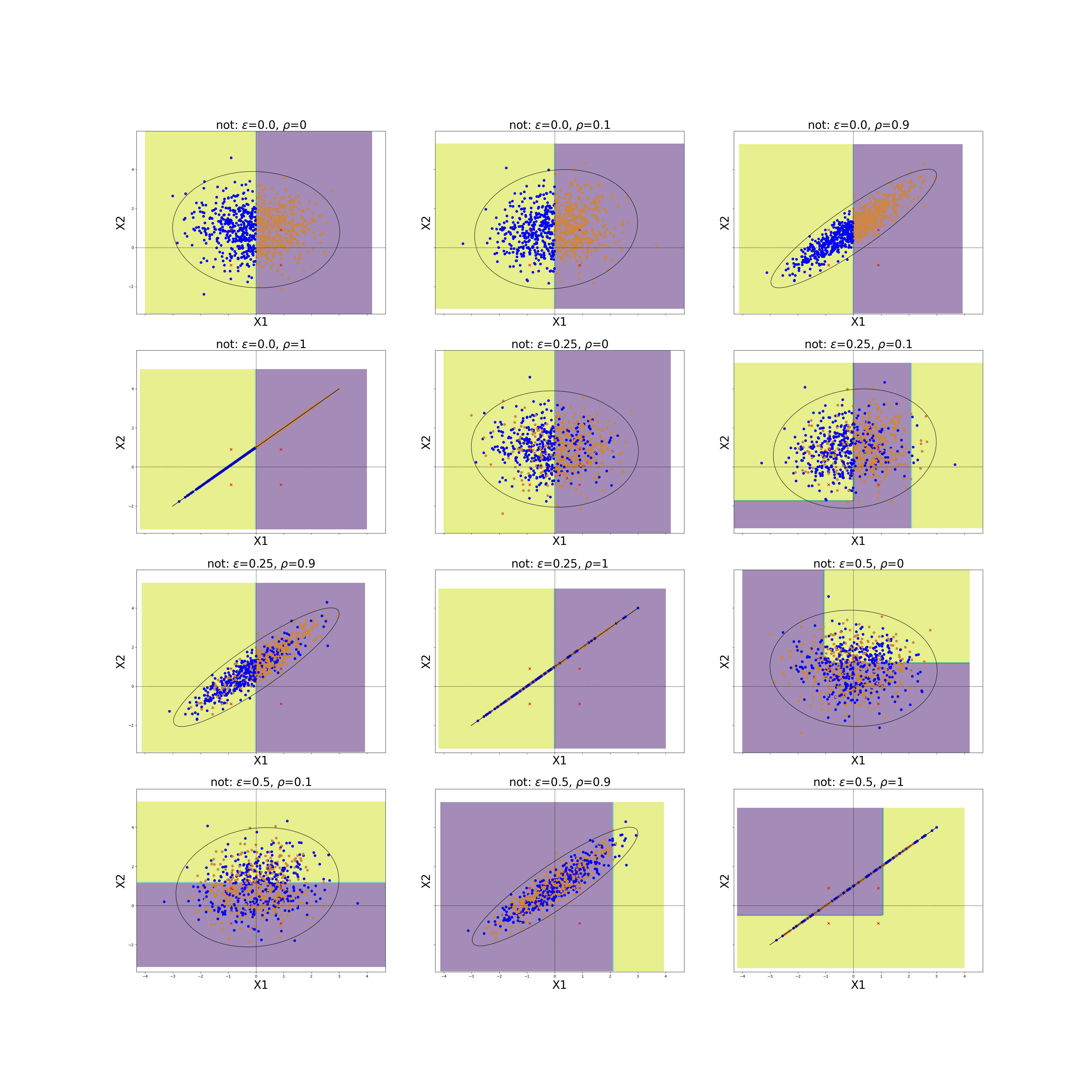
Partial-XOR and Partial-NOT exhibit feature independence (features are independent from each other – when the target is observed), and both features are required to make a perfect prediction for Partial-XOR, and only is required to perfectly predict Partial-NOT; in this case deterministic.
In real-world settings, Full represents the case where one feature is related to another feature and both participate to make the prediction of the output, for example in Adult Income dataset (that we later include in our experiments) the feature occupation is correlated to age and both predict the output income. Partial-CAUS on the other hand, may represent a causal relationship between one feature and the outcome through a chain of causality; or an indirect correlation of one feature on the output through another feature(or even multiple features), forming a chain of correlations.
Full and Partial-CAUS are specific cases of respectively Partial-XOR and Partial-NOT when is dependent on , thus for the rest of this paper, we denote XOR to refer to both Full and Partial-XOR, and use NOT to refer to Partial-CAUS and Partial-NOT. The data can be generated as:
Where is a bi-variate normal distribution and is the covariance matrix, representing the amount of correlation between the two random variables and . In order to introduce noise, we apply a mask to invert a percentage of labels in the output . Let’s denote the percentage of labels to invert as . Let be a binary mask defined as:
The perturbed output can be obtained with :
With and represents the logical operators XOR or NOT.
Ground truth feature importance
We use to denote the ground truth feature importance that are given by the true model to which we compare , the feature importance estimates that is generated by each of the local explainability methods to explain the predictions of the learned model . Intuitively, the true model can be illustrated with a -depth decision tree. With for XOR dataset variants (the first split on and the second on ) and for NOT dataset variants (only one split on ).
When , the ground truth feature importance for all variants of XOR datasets are fixed as = = .5, because both and are necessary to make the prediction of XOR. The amount of the correlation between and doesn’t affect the importance as both are necessary to make the prediction of XOR. Meanwhile, only is necessary to make the prediction of NOT, thus = 1 and = , because when is correlated to , have an indirect influence estimated by to predict NOT.
On the other hand, when , for XOR dataset variants, and and for NOT dataset variants.
For the XOR function, both and are equally important in determining the output, and their importance scores should ideally converge to when considering a large amount of data points. Consider a decision tree model that aims to predict the XOR function using features and . For simplicity, let’s assume that the decision tree splits on both and at each level. The decision tree’s predictions can be expressed as:
Now, let’s define the feature importance scores ( and ) using the Gini impurity criterion, a common metric for decision trees:
In a large dataset, the decision tree will be able to accurately capture the XOR relationship, and both and should contribute equally to the impurity decrease, leading to similar importance scores. For a balanced decision tree, these Gini decreases would be distributed among the splits involving and . In the limit of a large dataset, we would expect:
This indicates that, as the dataset size increases, the decision tree’s feature importance for predicting the XOR function would converge to for both and , reflecting their equal importance in determining the output.
5 Empirical Setup
To carry out our experiments, we demonstrate our findings on four real-world datasets: Heart Diagnosis, Cervical Cancer, Adult Income and German Credit Risk. These datasets include properties such as feature interactions (dependence or independence),noise, random irrelevant variables and class imbalance.
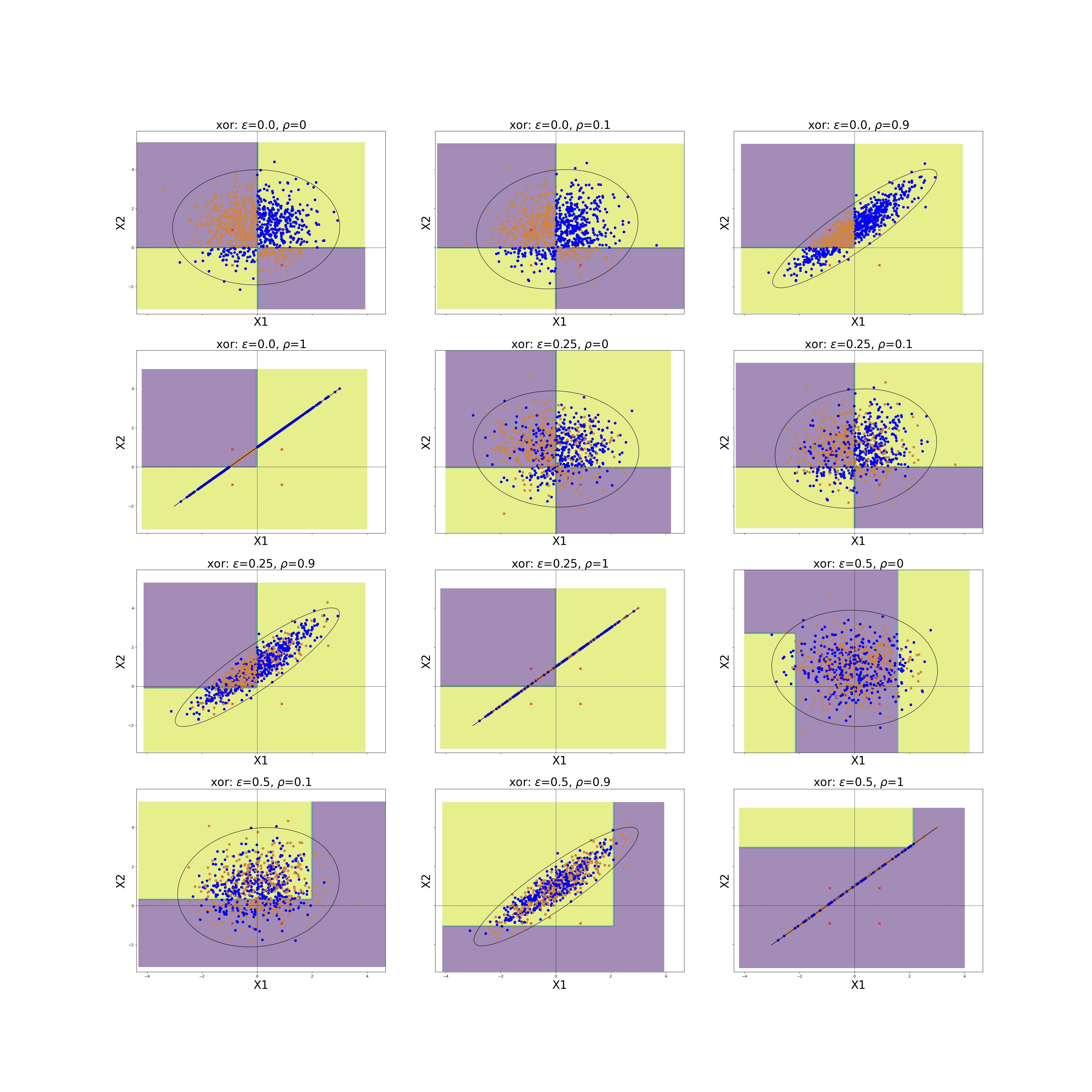
We generate 24 synthetic datasets (Figures 2 and 3) expressing different combinations of these properties by varying several parameters such as the correlation amount of the normal distribution from which the data points are drawn and the probability of each class, thus, the amount of generated noise and class imbalance. Each dataset is divided to 80% for training and 20% for testing. We report the results of the feature importance estimates on the test set. We compute feature importance estimates on the true model and learned model , so that we can compare the generated feature importance estimates to their ground truth values. Finally, we analyze the advantages and limitations of each explainability method on the synthetic datasets and we run larger experiments on the above real-world datasets from the UCI repository [37].
5.1 Datasets, models and metrics
Datasets
In addition, Table 2 summarizes the properties of the four real-world datasets that we use to demonstrate our findings.
| Dataset | instances | features | discrete | continuous | imbalance |
|---|---|---|---|---|---|
| Heart Diagnosis | 303 | 13 | 43 | 57 | yes |
| Cervical Cancer | 858 | 35 | 62 | 38 | yes |
| Adult Income | 32561 | 11 | 65 | 35 | no |
| German Credit Risk | 1 000 | 23 | 70 | 30 | yes |
Models
For the synthetic datasets, we compute the feature importance scores of the learned model on datasets with 1 000 instances. The learned model can be either a decision tree or a random forest.On the other hand, we use the random forest model with parameters learned using grid search and evaluated with 10-fold cross-validation for each of the real-world datasets. Table 3 summarizes the performances and the feature importance of the decision tree and the random forest models for the generated datasets.
| Decision function | DT Accuracy | DT feature importance | RF Accuracy | RF feature importance | ||
|---|---|---|---|---|---|---|
| XOR | 0.00 | 0.00 | 1.00 | =0.44, =0.56 | 0.85 | =0.69, =0.31 |
| XOR | 0.00 | 0.10 | 1.00 | =0.41, =0.59 | 0.90 | =0.63, =0.37 |
| XOR | 0.00 | 0.90 | 1.00 | =0.51, =0.49 | 1.00 | =0.55, =0.45 |
| XOR | 0.00 | 1.00 | 1.00 | =0.5, =0.5 | 1.00 | =0.53, =0.47 |
| XOR | 0.25 | 0.00 | 0.70 | =0.47, =0.53 | 0.61 | =0.62, =0.38 |
| XOR | 0.25 | 0.10 | 0.72 | =0.4, =0.6 | 0.62 | =0.64, =0.36 |
| XOR | 0.25 | 0.90 | 0.72 | =0.51, =0.49 | 0.72 | =0.56, =0.44 |
| XOR | 0.25 | 1.00 | 0.71 | =0.51, =0.49 | 0.71 | =0.53, =0.47 |
| XOR | 0.50 | 0.00 | 0.52 | =0.83, =0.17 | 0.50 | =0.57, =0.43 |
| XOR | 0.50 | 0.10 | 0.53 | =0.69, =0.31 | 0.56 | =0.57, =0.43 |
| XOR | 0.50 | 0.90 | 0.49 | =0.64, =0.36 | 0.46 | =0.53, =0.47 |
| XOR | 0.50 | 1.00 | 0.54 | =0.55, =0.45 | 0.47 | =0.53, =0.47 |
| NOT | 0.00 | 0.00 | 1.00 | =1.0, =0.0 | 1.00 | =0.84, =0.16 |
| NOT | 0.00 | 0.10 | 1.00 | =1.0, =0.0 | 1.00 | =0.83, =0.17 |
| NOT | 0.00 | 0.90 | 1.00 | =1.0, =0.0 | 1.00 | =0.61, =0.39 |
| NOT | 0.00 | 1.00 | 1.00 | =1.0, =0.0 | 1.00 | =0.49, =0.51 |
| NOT | 0.25 | 0.00 | 0.72 | =1.0, =0.0 | 0.72 | =0.77, =0.23 |
| NOT | 0.25 | 0.10 | 0.69 | =0.99, =0.01 | 0.72 | =0.8, =0.2 |
| NOT | 0.25 | 0.90 | 0.71 | =1.0, =0.0 | 0.71 | =0.63, =0.37 |
| NOT | 0.25 | 1.00 | 0.72 | =0.97, =0.03 | 0.72 | =0.49, =0.51 |
| NOT | 0.50 | 0.00 | 0.50 | =0.39, =0.61 | 0.48 | =0.55, =0.45 |
| NOT | 0.50 | 0.10 | 0.58 | =0.0, =1.0 | 0.57 | =0.5, =0.5 |
| NOT | 0.50 | 0.90 | 0.50 | =0.69, =0.31 | 0.46 | =0.53, =0.47 |
| NOT | 0.50 | 1.00 | 0.48 | =0.49, =0.51 | 0.50 | =0.51, =0.49 |
Metrics
To evaluate the quality of the feature importance estimates attributed by the methods in Table 1, we compare the feature importance estimates to the ground truth feature importance in Section 4 of the synthetic datasets because the ground truth feature importance estimates in the real-world datasets are hard to obtain. We also evaluate the stability, compactness, consistency, feature and rank agreements for the synthetic and real-world datasets.
5.2 Experiments
5.2.1 Synthetic data
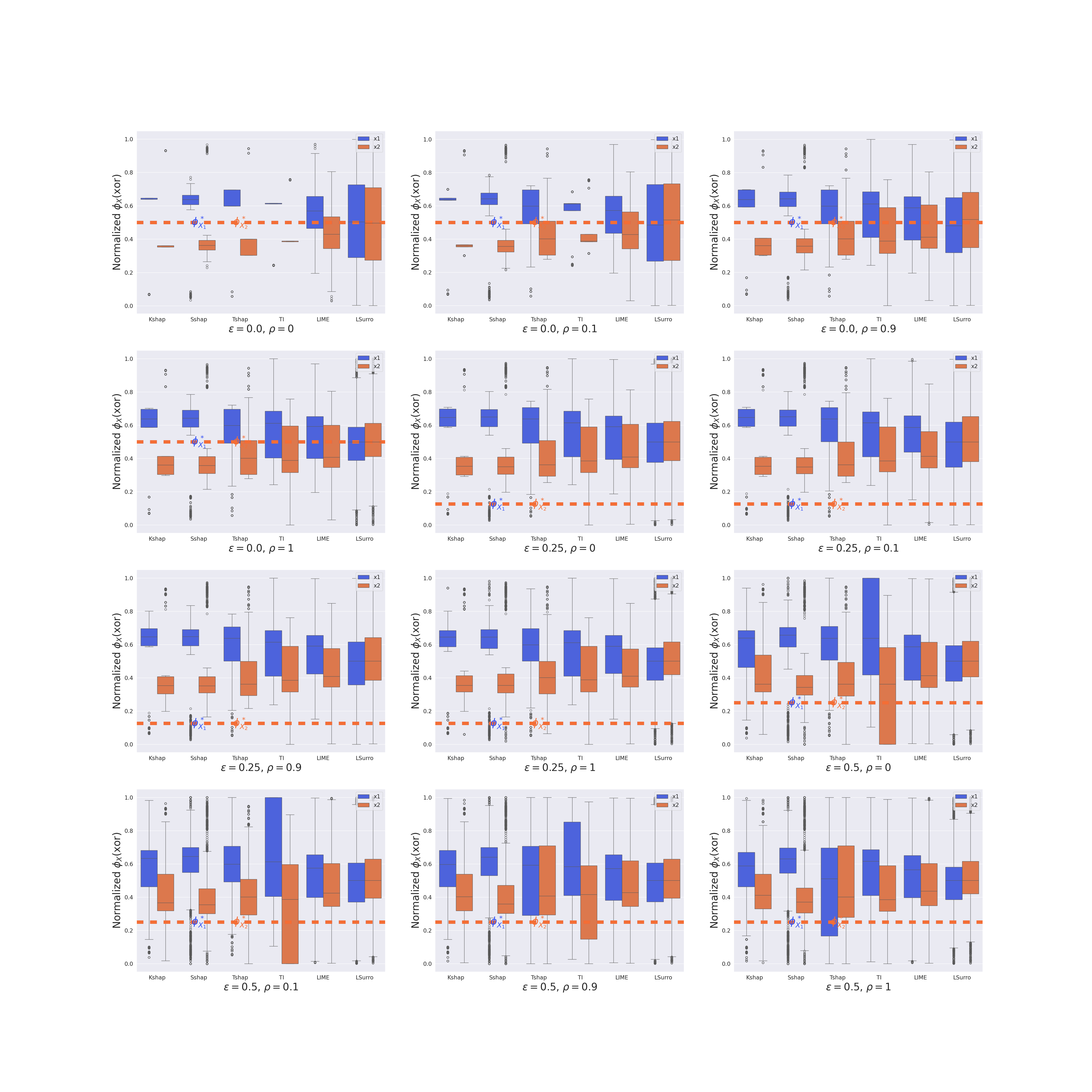
Figures 4 and 5 show the normalized feature importance estimates attributed by the selected explainability methods. After the normalization of the absolute importance of and , their contributions sum to one. We perform the normalization to faithfully compare the feature attributions to their ground truth values.
Explainability methods based on learning surrogate models overestimate the importance to irrelevant variables, Tree interpreter is sensitive to noise and SHAP explainers always favor one feature over the other
Overall, all explainers except local surrogates overestimate the importance of over across the XOR datasets. Also, none of these methods perfectly matches ground truth feature importance on average across all datasets. Moreover, LSurro and LIME feature importance attributions are the least affected by noise and feature correlation. Indeed, LSurro and and LIME attribute comparable importance to and for XOR and NOT dataset variants, and both overestimate the importance of unimportant features (such as in case of NOT). Notably, TI is the most affected by noise, that is confirmed in its decomposition of the the feature and noise contributions to the prediction. Additionally, feature correlations increase the importance and instability of importance in XOR datasets attributed by SHAP explainers, and noise lowers the importance of and for all the explainers. Finally, SHAP explainers and TI have the highest variance of feature importance estimates in the NOT datasets.

SHAP explainers yield very comparable explanations
Figure 6 shows the faithfulness of the explanations to the ground truth measured by mean consistency and mean feature agreements across the XOR and NOT generated datasets.
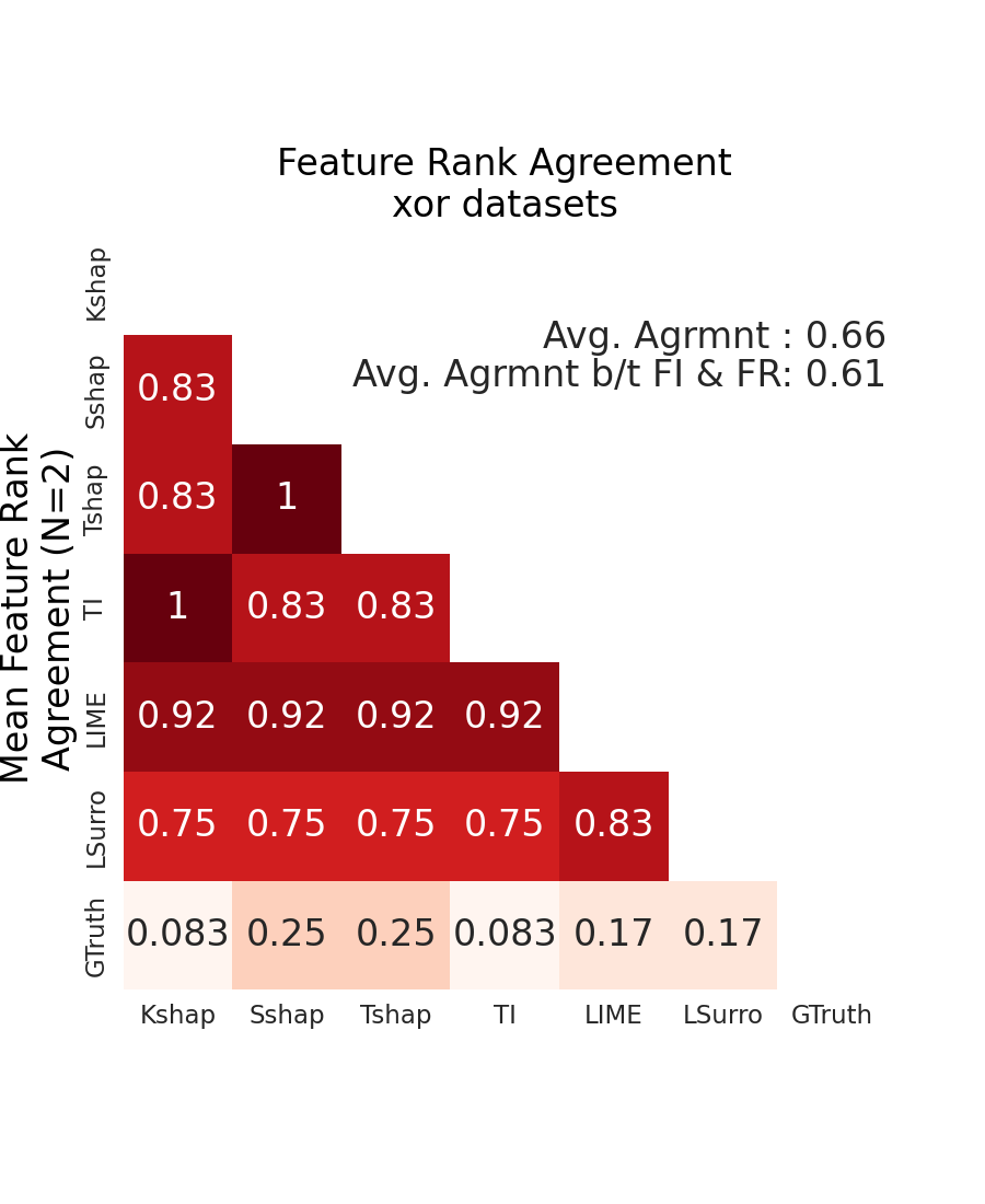
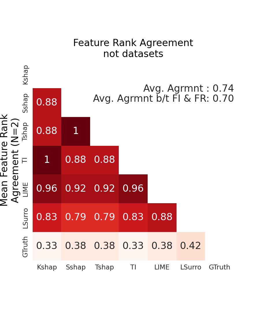
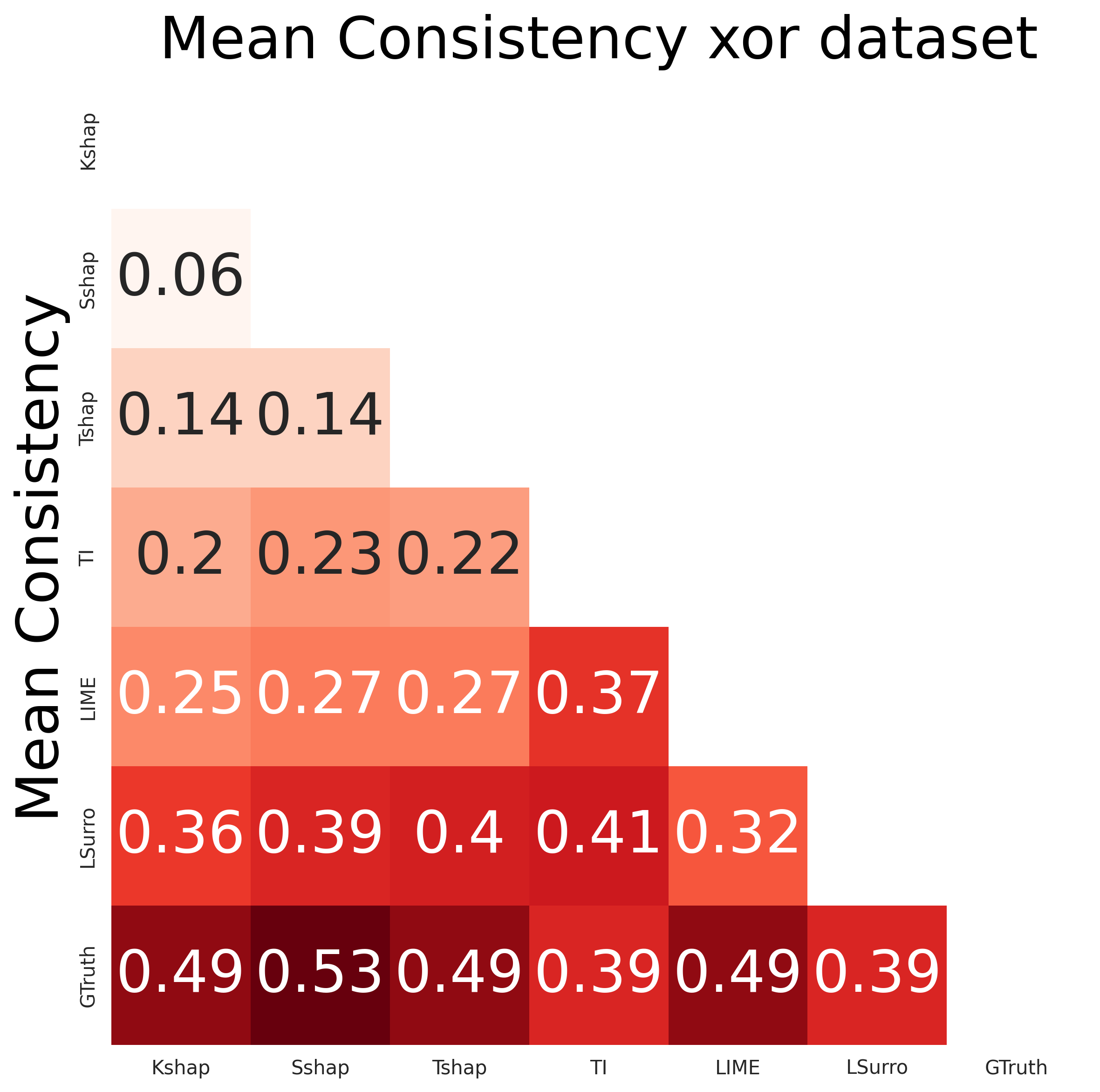
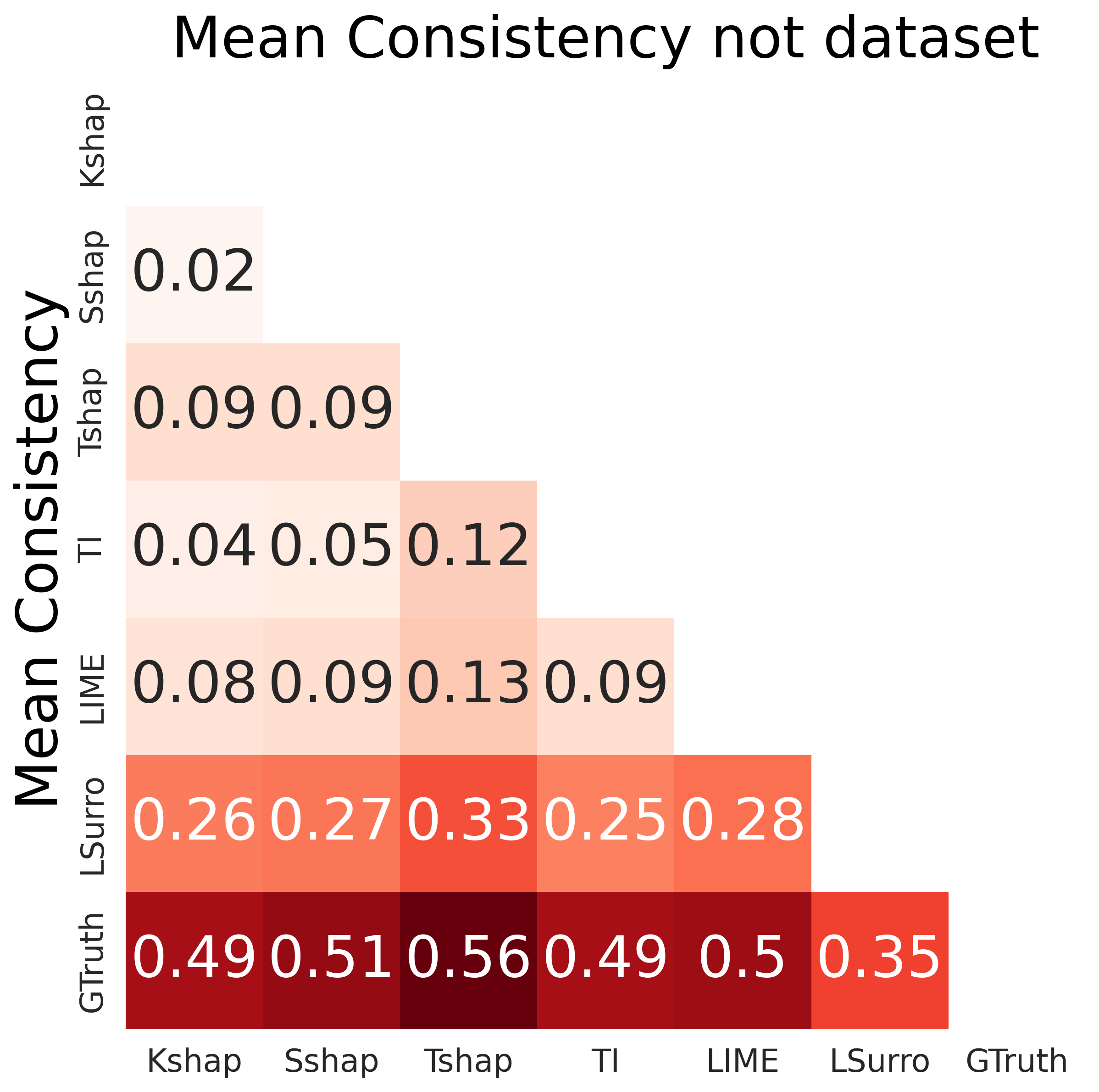
SHAP explainers yield consistent explanations due to the same feature importance attribution mechanism they all employ. However their explanations are the most inconsistent with respect to the ground truth values. Furthermore and for both XOR and NOT datasets, on average the fraction of common feature importance between TI and KShap and between SShap and TShap match perfectly.
| function | Methods | # Features for 90% approximation | Distance with 1 feature(%) | Mean consistency | Mean Stability (10) |
|---|---|---|---|---|---|
| XOR | Kshap | 1.00 | 0.10 | 0.21 | 0.21 |
| XOR | Sshap | 1.00 | 0.11 | 0.23 | 0.24 |
| XOR | Tshap | 1.00 | 0.10 | 0.24 | 0.25 |
| XOR | TI | 1.00 | 0.17 | 0.26 | 0.24 |
| XOR | LIME | 1.00 | 0.16 | 0.28 | 0.33 |
| XOR | LSurro | 1.33 | 0.43 | 0.32 | 0.15 |
| NOT | Kshap | 1.00 | 0.03 | 0.14 | 0.16 |
| NOT | Sshap | 1.00 | 0.03 | 0.15 | 0.20 |
| NOT | Tshap | 1.00 | 0.03 | 0.19 | 0.19 |
| NOT | TI | 1.00 | 0.02 | 0.15 | 0.19 |
| NOT | LIME | 1.00 | 0.04 | 0.17 | 0.27 |
| NOT | LSurro | 1.17 | 0.30 | 0.25 | 0.08 |
LSurro is the most locally stable, overestimates unimportant features and achieves better model accuracy with less features
Table 4 shows mean consistency, mean stability and compactness across the XOR and NOT datasets. For XOR and NOT datasets respectively, Kshap is the most consistent to the rest of the explanatory methods on average. Additionally, on average, LSurro generates the most locally stable explanations in XOR and NOT datasets, achieves higher model estimation and often consider both features as important fr both datasets.
5.2.2 Real-world data
For the real-world datasets the ground truth feature importance is unavailable, we perform evaluation of the different metrics in Section 2.
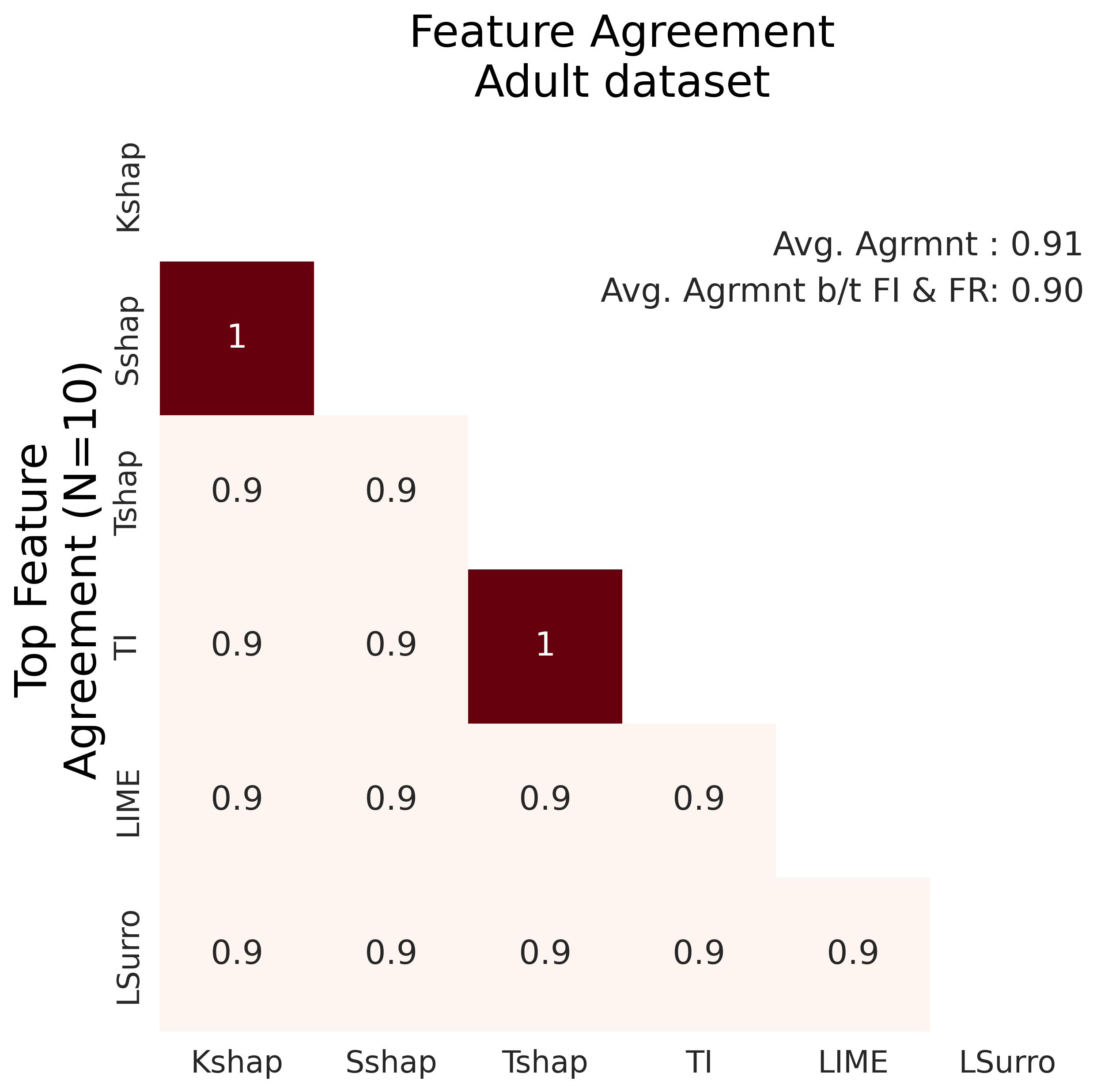
Local surrogates achieves 100% of model accuracy with 5 features on Adult Income dataset.
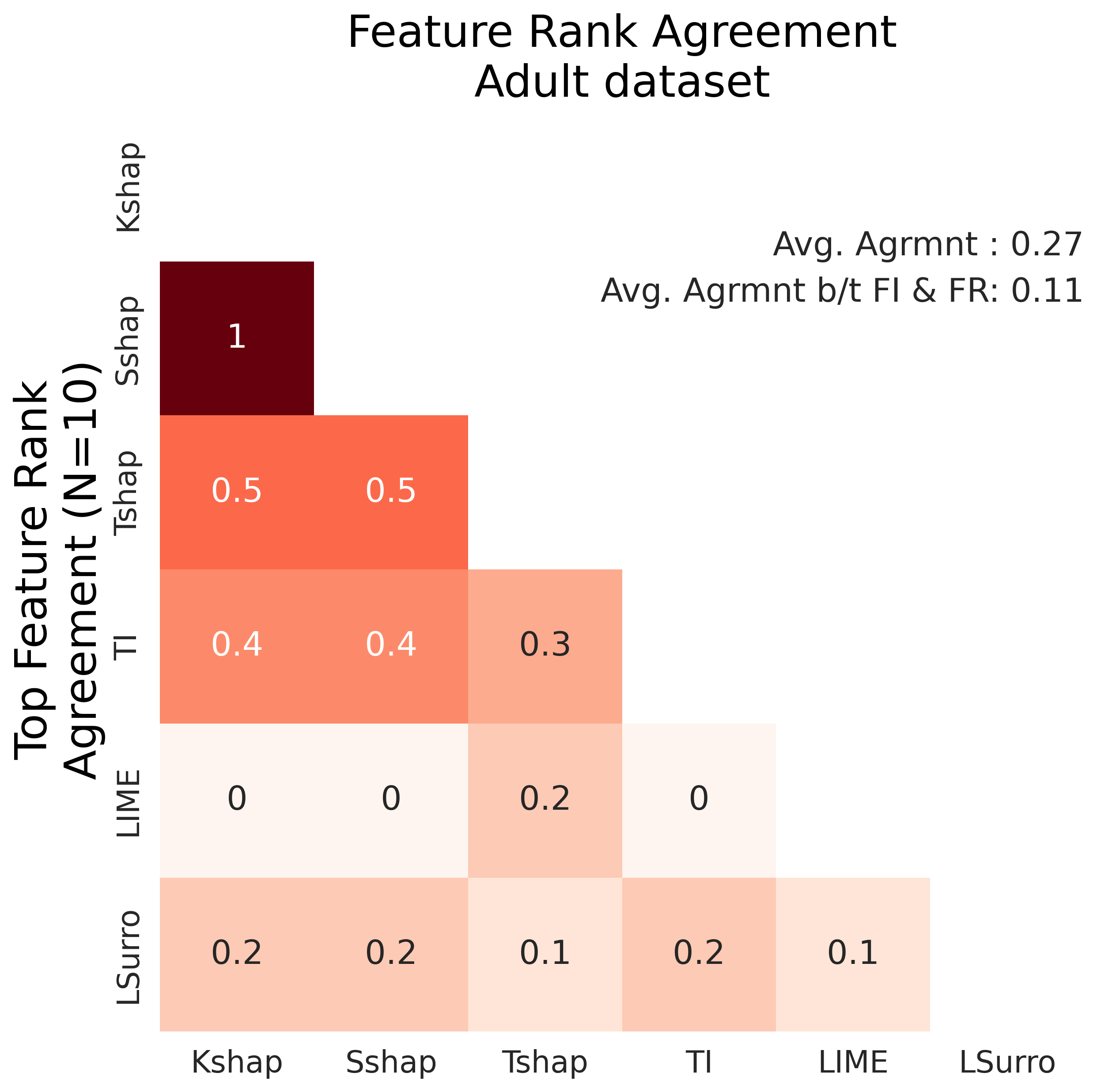
Figure 7 shows feature agreements for Adult Income Income dataset. Kshap and Sshap have exactly the same top-10 feature attributions and ranking. TI and Tshap share the same set of top-10 features. The rest of the explainers share 90% of the top 10 most important features. LIME share the lowest of top-10 important features with TI, Kshap and Sshap on the ranking of the top 10 features. Additionally, Table 5 illustrates the compactness, mean consistency and stability of the different methods on the Adult Income Income dataset. LSurro explains 100% of model output with only 5 features. Kshap, Tshap and TI are the most stable for this dataset and LIME have the highest mean consistency across all the datasets.
| Methods | # Features for 90% Accuracy | Accuracy with 5 feature(%) | Mean consistency | Mean Stability |
| Kshap | 1 | 09 | 0.43 | 0.00 |
| Tshap | 1 | 09 | 0.43 | 0.00 |
| Sshap | 1 | 08 | 0.43 | 0.01 |
| LIME | 1 | 07 | 0.15 | 0.07 |
| TI | 1 | 10 | 0.5 | 0.00 |
| LSurro | 3 | 100 | 0.7 | 0.01 |
SHAP explainers generate the most consistent explanations for German Credit Risk dataset.
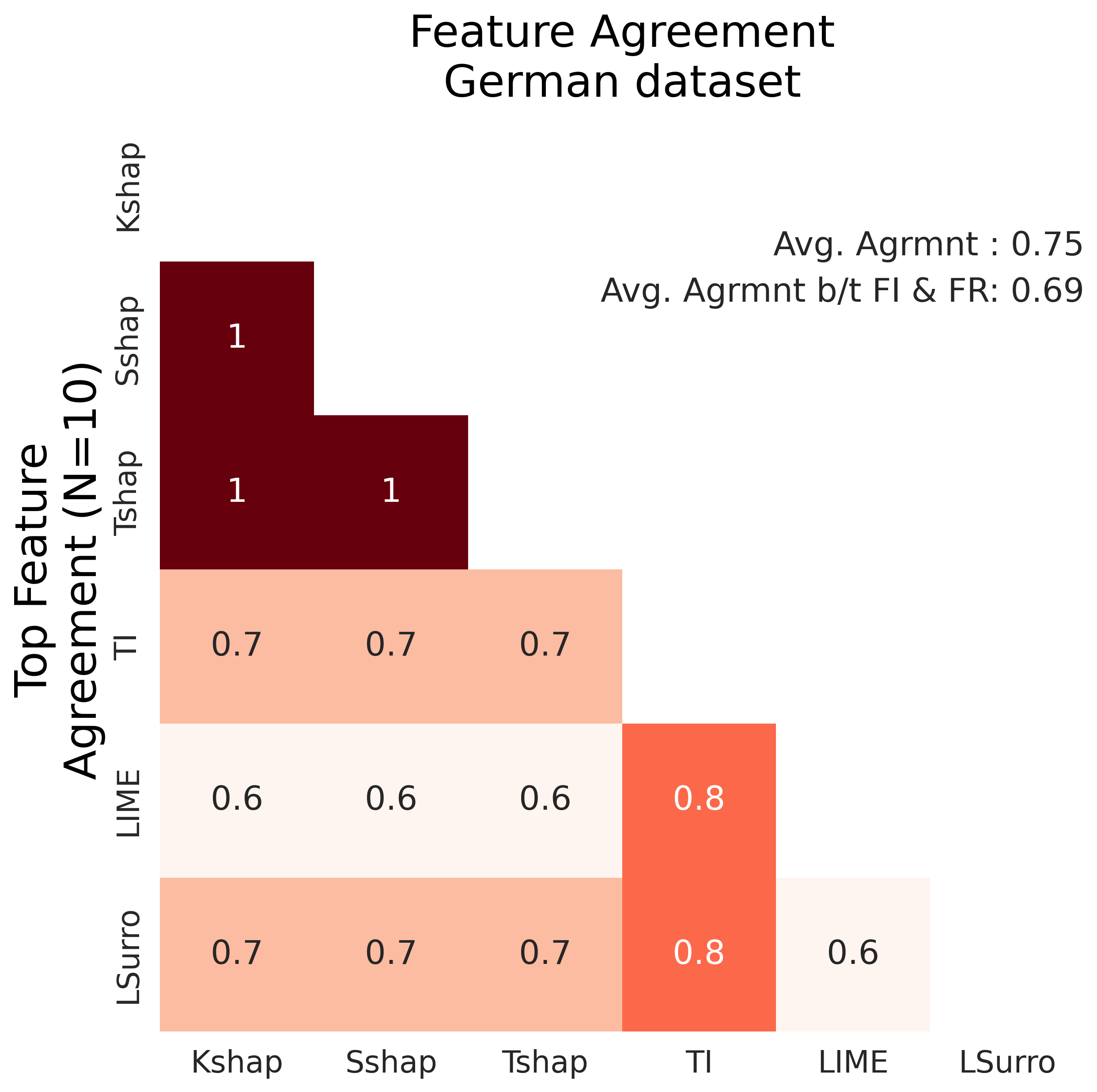
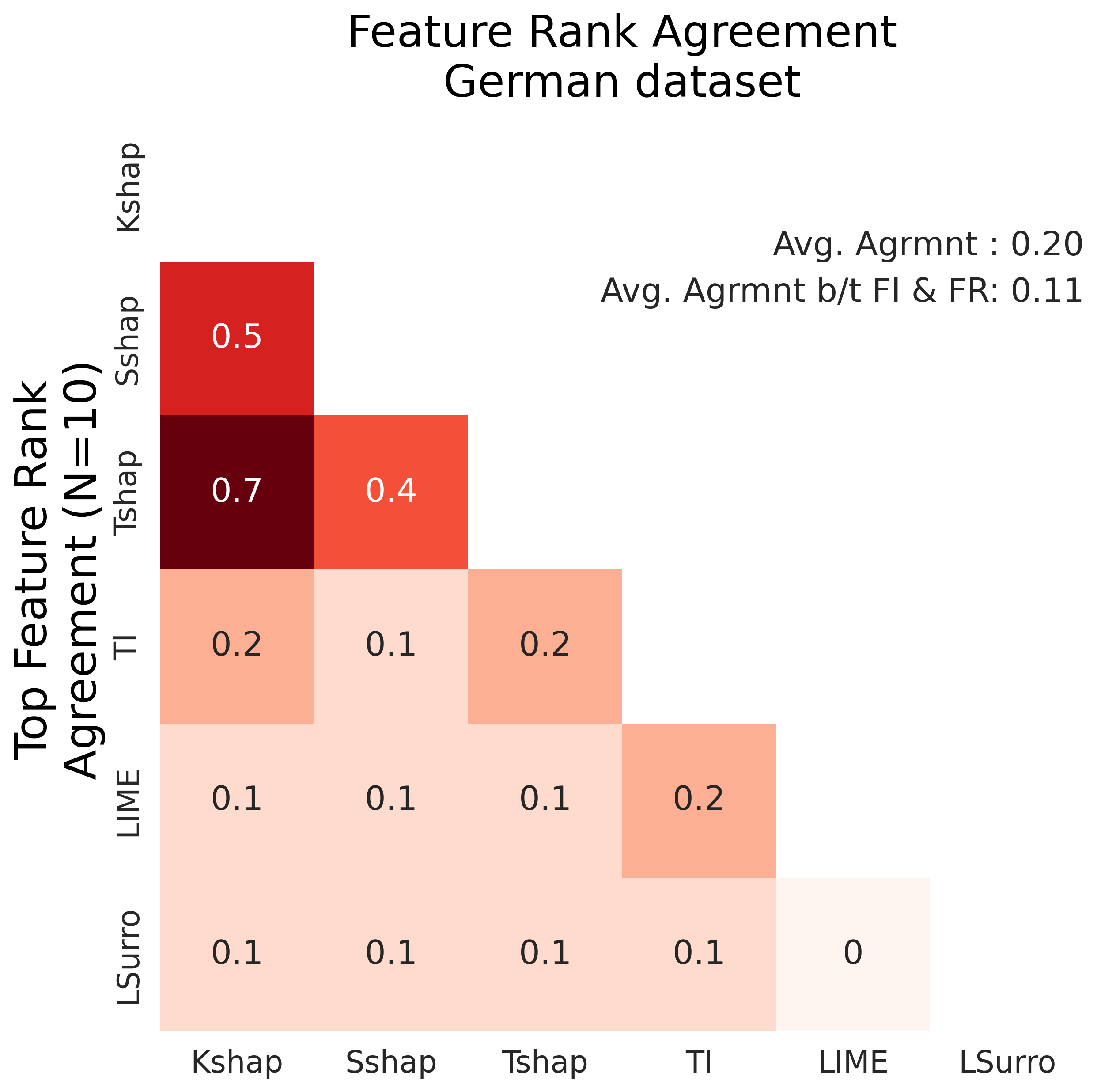
Figure 8 and Table 6 show the computed metrics on German Credit Risk dataset. Overall, all the explainers achieve 90% of model accuracy with only 1 feature and SHAP explainers are the most consistent among the methods. LIME is the most stable among the explainers. Moreover, SHAP explainers have same top-10 most important features as they all use the same mechanism of computation of the Shapley values the feature importance estimates, LIME have only 6 top features in common with SHAP explainers, and Kshap and Tshap share 7 features with the same rankings.
| Methods | # Features for 90% Accuracy | Accuracy with 5 feature(%) | Mean consistency | Mean Stability |
| Kshap | 1 | 12 | 0.45 | 0.03 |
| Tshap | 1 | 13 | 0.45 | 0.03 |
| Sshap | 1 | 12 | 0.45 | 0.03 |
| LIME | 1 | 41 | 1.18 | 0.00 |
| TI | 1 | 13 | 0.54 | 0.02 |
| LSurro | 1 | 57 | 0.74 | 0.03 |
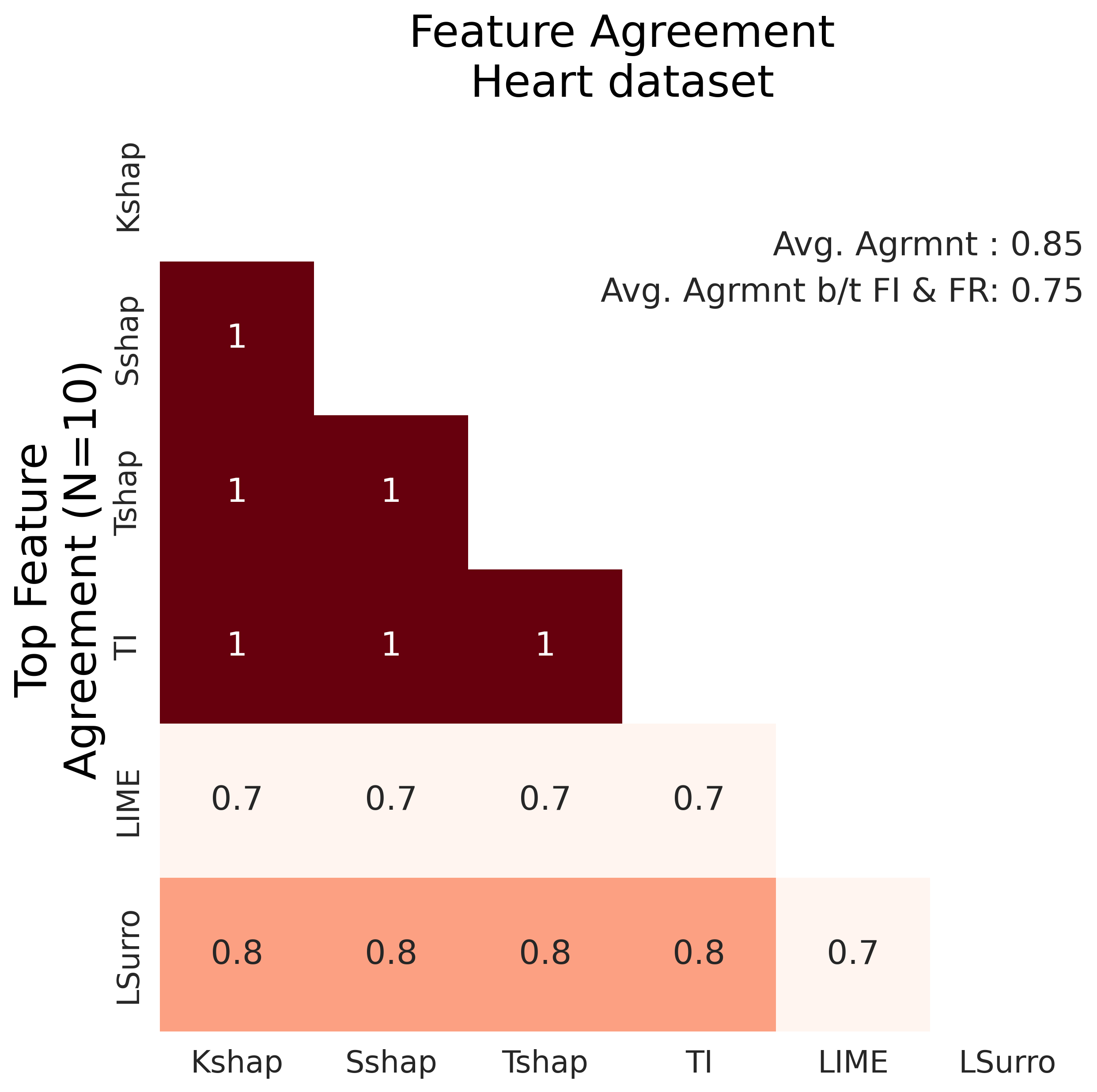
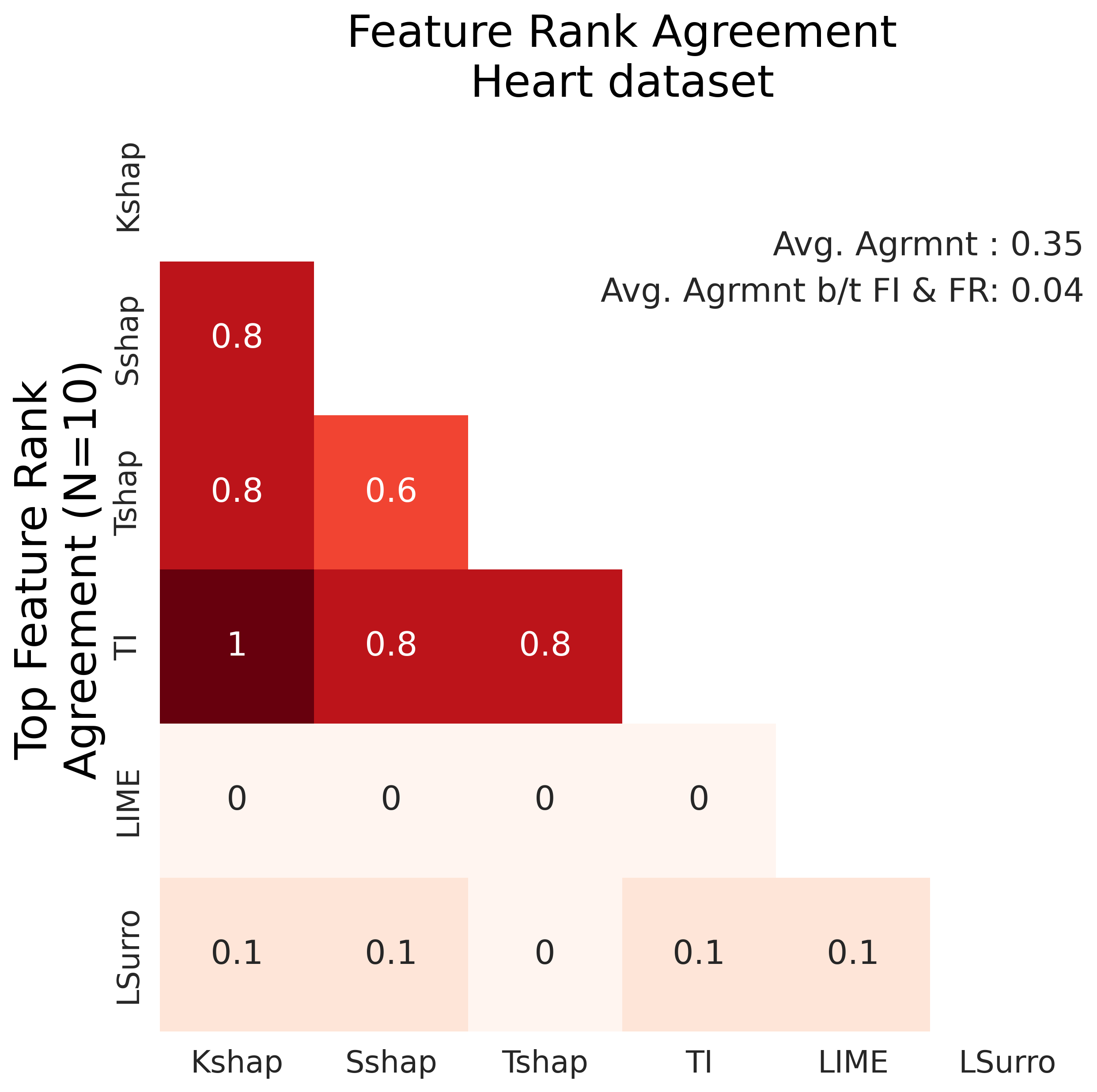
SHAP explainers and TI share the top-10 most important feature for Heart Diagnosis dataset
In Figure 9 and Table 7, SHAP explainers and TI share the top-10 most important feature, contrary to LIME which doesn’t share same ranking of the top features with other explainers. Kshap and TI have exactly the same top-10 features and in the same rankings. On the other hand, LSurro estimates 100% of model accuracy with only 5 features and SHAP explainers and TI generate the most stable and consistent explanations.
| Methods | # Features for 90% Accuracy | Accuracy with 5 feature(%) | Mean consistency | Mean Stability |
| Kshap | 1 | 18 | 0.4 | 0.00 |
| Tshap | 1 | 21 | 0.4 | 0.00 |
| Sshap | 1 | 18 | 0.4 | 0.00 |
| LIME | 1 | 31 | 1.2 | 0.03 |
| TI | 1 | 25 | 0.45 | 0.00 |
| LSurro | 6 | 100 | 0.63 | 0.03 |
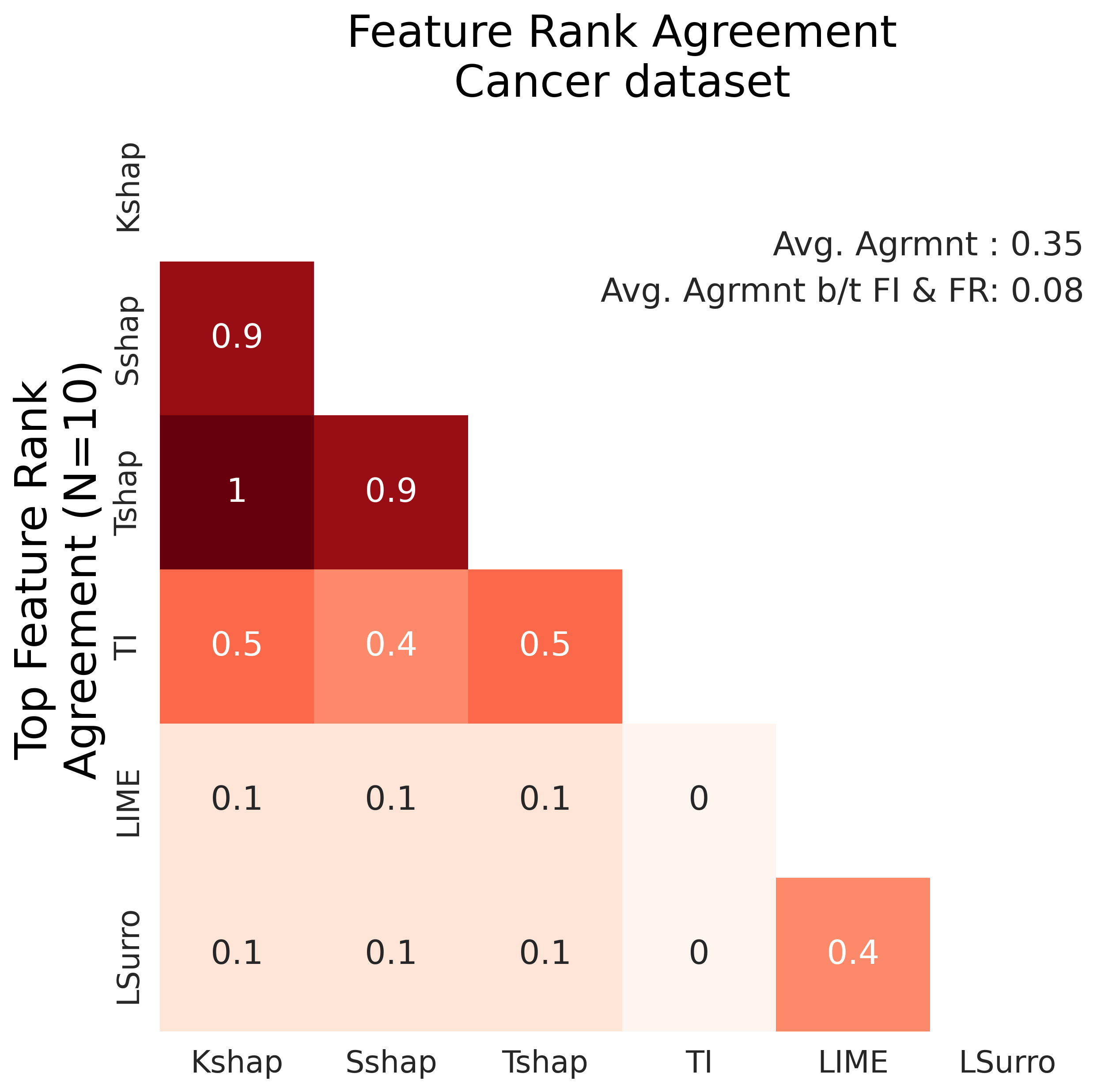
Local surrogates are the most consistent and explains 100% of model output with 5 features for Cervical Cancer dataset.
Figure 10 and Table 8 illustrate above metrics on the Cervical Cancer dataset. Tshap and Kshap share the top 10 features. LIME and Sshap have the lowest top features in common. LIME and LSurro have no comparable rankings of the the features with TI, although they both learn a surrogate linear model in the neighborhood of each instance but use different mechanisms of the generation of the local neighborhood, which can explain the disagreement in their features importance estimates. Additionally, LSurro is the most consistent and explains 100% of model output with 5 features, and SHAP explainers have the highest mean stability.

| Methods | # Features for 90% Accuracy | Accuracy with 5 feature(%) | Mean consistency | Mean Stability |
| Kshap | 1 | 12 | 1.44 | 0.34 |
| Sshap | 1 | 12 | 0.87 | 0.34 |
| Tshap | 1 | 12 | 0.36 | 0.34 |
| LIME | 1 | 45 | 0.66 | 0.46 |
| TI | 1 | 19 | 0.59 | 0.42 |
| LSurro | 3 | 100 | 0.22 | 0.54 |
6 Conclusions and Future Work
The experiments on the synthetic and real-world datasets showed that feature importance attribution can be affected by multiple factors such as data properties, the black-box model and the assumptions on which the explainable method is built to attribute feature contributions. We restricted our study to the first factor with a focus on some data properties, decision tree based models, on tabular data and for a binary classification task. For the matter of simplicity and ease of understanding of the model’s behavior, we restricted our generation model to two variables in order to easily track the feature interactions, which can be a limit in real-world scenarios because of the need to handle high-dimensional data in many situations.
-
•
For datasets with irrelevant variables, avoid using LSurro and LIME because both overestimate the importance of unimportant features.
-
•
We recommend to avoid using TI for highly noisy datasets because TI is the most unstable compared to other explainers in such datasets. This can be justified by the decomposition of of the feature importance used by TI, which allocates importance to the noise.
-
•
Kernel, Sampling and Tree SHAP explainers give very similar explanations, thus we recommend using Sshap or Tshap for faster computations and adaptability for decision trees.
Perspectives
Future work should further focus on each single explainability method separately to be able to explore in depth the effect of its assumptions and its inner workings for a single model parameter and on one specific data property on the feature importance attribution. Also, it is of interest to assess these feature importance estimates on other data parameters such as the number of instances in the test set and the number of features. Our work can be applied on other tasks such as regression and multi-class classification, to image and text data.
References
- \bibcommenthead
- Breiman [2001] Breiman, L.: Random Forests. Machine Learning 45(1), 5–32 (2001)
- Kulmala et al. [2017] Kulmala, L., Read, J., Nöjd, P., Rathgeber, C.B.K., Cuny, H.E., Hollmén, J., Mäkinen, H.: Identifying the main drivers for the production and maturation of scots pine tracheids along a temperature gradient. Agricultural and Forest Meteorology 232(January), 210–224 (2017)
- Ricordeau and Lacaille [2010] Ricordeau, J., Lacaille, J.: Application of Random Forests to Engine health Monitoring. (2010)
- Strobl et al. [2007] Strobl, C., Boulesteix, A.-L., Zeileis, A., Hothorn, T.: Bias in random forest variable importance measures: Illustrations, sources and a solution. BMC Bioinformatics 8(1), 25 (2007)
- [5] Terence, P., Prince, G.: Beware Default Random Forest Importances. http://explained.ai/decision-tree-viz/index.html
- Molnar et al. [2020] Molnar, C., Gruber, S., Kopper, P.: Limitations of Interpretable Machine Learning Methods, (2020)
- Ribeiro et al. [2016] Ribeiro, M.T., Singh, S., Guestrin, C.: ”Why Should I Trust You?”: Explaining the Predictions of Any Classifier. In: Proceedings of the 22nd ACM SIGKDD International Conference on Knowledge Discovery and Data Mining. KDD ’16, pp. 1135–1144. Association for Computing Machinery, New York, NY, USA (2016)
- Lundberg and Lee [2017] Lundberg, S., Lee, S.-I.: A Unified Approach to Interpreting Model Predictions. arXiv:1705.07874 [cs, stat] (2017) arXiv:1705.07874 [cs, stat]
- Krishna et al. [2022] Krishna, S., Han, T., Gu, A., Pombra, J., Jabbari, S., Wu, S., Lakkaraju, H.: The Disagreement Problem in Explainable Machine Learning: A Practitioner’s Perspective. arXiv (2022)
- Attanasio et al. [2022] Attanasio, G., Pastor, E., Di Bonaventura, C., Nozza, D.: Ferret: A Framework for Benchmarking Explainers on Transformers. arXiv (2022)
- Camburu et al. [2019] Camburu, O.-M., Giunchiglia, E., Foerster, J., Lukasiewicz, T., Blunsom, P.: Can I Trust the Explainer? Verifying Post-hoc Explanatory Methods. arXiv (2019)
- Bodria et al. [2021] Bodria, F., Giannotti, F., Guidotti, R., Naretto, F., Pedreschi, D., Rinzivillo, S.: Benchmarking and Survey of Explanation Methods for Black Box Models. arXiv (2021)
- Neely et al. [2021] Neely, M., Schouten, S.F., Bleeker, M.J.R., Lucic, A.: Order in the Court: Explainable AI Methods Prone to Disagreement. arXiv (2021)
- Flora et al. [2022] Flora, M., Potvin, C., McGovern, A., Handler, S.: Comparing explanation methods for traditional machine learning models part 1: An overview of current methods and quantifying their disagreement. arXiv preprint arXiv:2211.08943 (2022)
- Molnar [2022] Molnar, C.: Interpretable Machine Learning, 2nd edn. (2022). https://christophm.github.io/interpretable-ml-book
- Lundberg et al. [2019] Lundberg, S.M., Erion, G.G., Lee, S.-I.: Consistent Individualized Feature Attribution for Tree Ensembles. arXiv (2019)
- Li et al. [2019] Li, X., Wang, Y., Basu, S., Kumbier, K., Yu, B.: A Debiased MDI Feature Importance Measure for Random Forests. arXiv:1906.10845 [cs, stat] (2019). arXiv: 1906.10845. Accessed 2019-10-18
- Alvarez-Melis and Jaakkola [2018] Alvarez-Melis, D., Jaakkola, T.S.: On the Robustness of Interpretability Methods. arXiv (2018)
- Rajbahadur et al. [2022] Rajbahadur, G.K., Wang, S., Kamei, Y., Hassan, A.E.: The impact of feature importance methods on the interpretation of defect classifiers. IEEE Transactions on Software Engineering 48(7), 2245–2261 (2022) arXiv:2202.02389 [cs]
- Slack et al. [2021] Slack, D., Hilgard, S., Singh, S., Lakkaraju, H.: Reliable Post Hoc Explanations: Modeling Uncertainty in Explainability. arXiv (2021)
- Petsiuk et al. [2018] Petsiuk, V., Das, A., Saenko, K.: RISE: Randomized Input Sampling for Explanation of Black-box Models. arXiv (2018)
- [22] Bodria, F., Giannotti, F., Guidotti, R., Naretto, F., Pedreschi, D., Rinzivillo, S.: Benchmarking and survey of explanation methods for black box models 37(5), 1719–1778
- Liu et al. [2021a] Liu, Y., Khandagale, S., White, C., Neiswanger, W.: Synthetic Benchmarks for Scientific Research in Explainable Machine Learning. arXiv (2021)
- Liu et al. [2021b] Liu, Y., Khandagale, S., White, C., Neiswanger, W.: Synthetic benchmarks for scientific research in explainable machine learning. arXiv preprint arXiv:2106.12543 (2021)
- Han et al. [2022] Han, T., Srinivas, S., Lakkaraju, H.: Which Explanation Should I Choose? A Function Approximation Perspective to Characterizing Post Hoc Explanations. arXiv (2022)
- [26] Turbé, H., Bjelogrlic, M., Lovis, C., Mengaldo, G.: Evaluation of post-hoc interpretability methods in time-series classification 5(3), 250–260
- [27] Ismail, A.A., Gunady, M., Corrada Bravo, H., Feizi, S.: Benchmarking Deep Learning Interpretability in Time Series Predictions. In: Advances in Neural Information Processing Systems, vol. 33, pp. 6441–6452. Curran Associates, Inc.
- Yang and Kim [2019] Yang, M., Kim, B.: Benchmarking attribution methods with relative feature importance. arXiv preprint arXiv:1907.09701 (2019)
- Zhong et al. [2023] Zhong, Z., Liu, Z., Tegmark, M., Andreas, J.: The clock and the pizza: Two stories in mechanistic explanation of neural networks. arXiv preprint arXiv:2306.17844 (2023)
- Han et al. [2022] Han, T., Srinivas, S., Lakkaraju, H.: Which explanation should i choose? a function approximation perspective to characterizing post hoc explanations. Advances in Neural Information Processing Systems 35, 5256–5268 (2022)
- [31] Agarwal, C., Krishna, S., Saxena, E., Pawelczyk, M., Johnson, N., Zitnik, M., Lakkaraju, H.: OpenXAI: Towards a Transparent Evaluation of Post hoc Model Explanations, 16
- Kokhlikyan et al. [2020] Kokhlikyan, N., Miglani, V., Martin, M., Wang, E., Alsallakh, B., Reynolds, J., Melnikov, A., Kliushkina, N., Araya, C., Yan, S., Reblitz-Richardson, O.: Captum: A Unified and Generic Model Interpretability Library for PyTorch. arXiv (2020)
- Hedström et al. [2022] Hedström, A., Weber, L., Bareeva, D., Motzkus, F., Samek, W., Lapuschkin, S., Höhne, M.M.-C.: Quantus: An Explainable AI Toolkit for Responsible Evaluation of Neural Network Explanations. arXiv (2022)
- Guidotti [2021] Guidotti, R.: Evaluating local explanation methods on ground truth. Artificial Intelligence 291, 103428 (2021)
- Le et al. [2023] Le, P.Q., Nauta, M., Van Bach Nguyen, S.P., Schlötterer, J., Seifert, C.: Benchmarking explainable ai-a survey on available toolkits and open challenges. In: International Joint Conference on Artificial Intelligence (2023)
- Turbé et al. [2023] Turbé, H., Bjelogrlic, M., Lovis, C., Mengaldo, G.: Evaluation of post-hoc interpretability methods in time-series classification. Nature Machine Intelligence 5(3), 250–260 (2023)
- Dua and Graff [2017] Dua, D., Graff, C.: UCI Machine Learning Repository (2017). http://archive.ics.uci.edu/ml