Nonequispaced fast Fourier transforms for bandlimited functions

Abstract

In this paper we consider the problem of approximating function evaluations $f(\boldsymbol{x}_{j})$ at given nonequispaced points $\boldsymbol{x}_{j}$, $j=1,\dots N$, of a bandlimited function from given values $\hat{f}(\boldsymbol{k})$, $\boldsymbol{k}\in\mathcal{I}_{\boldsymbol{M}}$, of its Fourier transform. Note that if a trigonometric polynomial is given, it is already known that this problem can be solved by means of the nonequispaced fast Fourier transform (NFFT). In other words, we introduce a new NFFT-like procedure for bandlimited functions, which is based on regularized Shannon sampling formulas.

Key words: nonequispaced fast Fourier transform, bandlimited functions, regularized Shannon sampling formulas, sinc function, NFFT, NUFFT

AMS Subject Classifications: 65Txx, 65T50, 94A20

1 Introduction

The nonequispaced fast Fourier transform (NFFT) is a fast algorithm to evaluate a trigonometric polynomial

$$f(\boldsymbol{x})=\sum_{\boldsymbol{k}\in\mathcal{I}_{\boldsymbol{M}}}\hat{f}_{\boldsymbol{k}}\,\mathrm{e}^{2\pi\mathrm{i}\boldsymbol{k}\boldsymbol{x}},\quad\boldsymbol{x}\in\mathbb{T}^{d},$$

with given Fourier coefficients $\hat{f}_{\boldsymbol{k}}\in\mathbb{C}$, $\boldsymbol{k}\in\mathcal{I}_{\boldsymbol{M}}$, at given nonequispaced points $\boldsymbol{x}_{j}\in\mathbb{T}^{d}$, $j=1,\dots,N$, $N\in\mathbb{N}$, where for $\boldsymbol{M}\coloneqq(M,\dots,M)^{T}$, $M\in 2\mathbb{N}$, we define the index set $\mathcal{I}_{\boldsymbol{M}}\coloneqq\mathbb{Z}^{d}\cap\left[-\tfrac{M}{2},\tfrac{M}{2}\right)^{d}$ with cardinality $|\mathcal{I}_{\boldsymbol{M}}|=M^{d}$, and $\mathbb{T}^{d}\coloneqq\mathbb{R}^{d}\setminus\mathbb{Z}^{d}$ denotes the $d$-dimensional torus with $d\in\mathbb{N}$.

In this paper we focus on the analogous problem for bandlimited functions, where we aim to approximate evaluations $f(\boldsymbol{x}_{j})$, $j=1,\dots,N$, of a function

$$f(\boldsymbol{x})=\int\limits_{\left[-\frac{M}{2},\frac{M}{2}\right)^{d}}\hat{f}(\boldsymbol{v})\,\mathrm{e}^{2\pi\mathrm{i}\boldsymbol{v}\boldsymbol{x}}\,\mathrm{d}\boldsymbol{v},\quad\boldsymbol{x}\in\mathbb{R}^{d},$$ (1.1)

from given measurements $\hat{f}(\boldsymbol{k})\in\mathbb{C}$, $\boldsymbol{k}\in\mathcal{I}_{\boldsymbol{M}}$, of its functions Fourier transform $\hat{f}$.

To do so, this paper is organized as follows. Firstly, in Section 2 we review the NFFT for trigonometric polynomials. Subsequently, in Section 3 we give an overview of the regularized Shannon sampling formulas, which play the key role in introducing the NFFT-like procedure for bandlimited functions in Section 4. Finally, in Section 5 we compare this new method to the classical NFFT.

2 The NFFT

For given nonequispaced nodes $\boldsymbol{x}_{j}\in\mathbb{T}^{d}$,  $j=1,\dots,N$, and given coefficients $\hat{f}_{\boldsymbol{k}}\in\mathbb{C}$, $\boldsymbol{k}\in\mathcal{I}_{\boldsymbol{M}}$, we consider the computation of the sums

$$f(\boldsymbol{x}_{j})=\sum_{\boldsymbol{k}\in\mathcal{I}_{\boldsymbol{M}}}\hat{f}_{\boldsymbol{k}}\,\mathrm{e}^{2\pi\mathrm{i}\boldsymbol{k}\boldsymbol{x}_{j}},\quad j=1,\dots,N,$$ (2.1)

where the inner product of two vectors shall be defined as usual as $\boldsymbol{k}\boldsymbol{x}\coloneqq k_{1}x_{1}+\dots+k_{d}x_{d}$. A fast approximate algorithm, the so-called nonequispaced fast Fourier transform (NFFT), can be summarized as follows, see e. g. [6, 2, 27, 9, 12] or [21, pp. 413–417].

Algorithm 2.1 (NFFT).

 

For $d,N\in\mathbb{N}$ and $\boldsymbol{M}=(M_{1},\dots,M_{d})^{\top}\in(2\mathbb{N})^{d}$ let $\boldsymbol{x}_{j}\in\mathbb{T}^{d},\,j=1,\dots,N,$ be given nodes as well as $\hat{f}_{\boldsymbol{k}}\in\mathbb{C}$, $\boldsymbol{k}\in\mathcal{I}_{\boldsymbol{M}}$, given Fourier coefficients. Furthermore, we are given the $d$-dimensional oversampling factor $\boldsymbol{\sigma}\geq\boldsymbol{1}_{d}$, the vector $\boldsymbol{M}_{\boldsymbol{\sigma}}\coloneqq((M_{\sigma})_{1},\dots,(M_{\sigma})_{d})^{\top}$ with $2\mathbb{N}\ni(M_{\sigma})_{t}\coloneqq 2\lceil\,\lceil\sigma_{t}M_{t}\rceil/2\,\rceil$, as well as the window function $\varphi$, the truncated function $\varphi_{m}$ with $m\ll(M_{\sigma})_{t}$, $t=1,\dots,d$, and their $1$-periodic versions $\tilde{\varphi}$ and $\tilde{\varphi}_{m}$.

1. Precomputation:

   1. Compute the nonzero Fourier coefficients $\hat{\varphi}(\boldsymbol{k})$ for $\boldsymbol{k}\in\mathcal{I}_{\boldsymbol{M}}$.

   2. Compute the nonzero values $\tilde{\varphi}_{m}\hskip-2.5pt\left(\boldsymbol{x}_{j}-\boldsymbol{M}_{\boldsymbol{\sigma}}^{-1}\odot\boldsymbol{\ell}\right)$ for $j=1,\dots,N,$ as well as $\boldsymbol{\ell}\in\mathcal{I}_{\boldsymbol{M_{\boldsymbol{\sigma}}},m}(\boldsymbol{x}_{j})$, cf. (2.5).

2. Set $\mathcal{O}(|\mathcal{I}_{\boldsymbol{M}}|)$

   $$\hat{g}_{\boldsymbol{k}}\coloneqq\left\{\begin{array}[]{cl}\frac{\hat{f}_{\boldsymbol{k}}}{\hat{\varphi}(\boldsymbol{k})}&\colon\boldsymbol{k}\in\mathcal{I}_{\boldsymbol{M}},\\ 0&\colon\boldsymbol{k}\in\mathcal{I}_{\boldsymbol{M_{\boldsymbol{\sigma}}}}\setminus\mathcal{I}_{\boldsymbol{M}}.\end{array}\right.$$

3. Compute

   $$g_{\boldsymbol{\ell}}\coloneqq\frac{1}{|\mathcal{I}_{\boldsymbol{M_{\boldsymbol{\sigma}}}}|}\sum_{\boldsymbol{k}\in\mathcal{I}_{\boldsymbol{M}}}\hat{g}_{\boldsymbol{k}}\,\mathrm{e}^{2\pi\mathrm{i}\boldsymbol{k}(\boldsymbol{M}_{\boldsymbol{\sigma}}^{-1}\odot\,\boldsymbol{\ell})},\quad\boldsymbol{\ell}\in\mathcal{I}_{\boldsymbol{M_{\boldsymbol{\sigma}}}},$$

   by means of a $d$-variate iFFT. $\mathcal{O}(|\mathcal{I}_{\boldsymbol{M}}|\log(|\mathcal{I}_{\boldsymbol{M}}|))$

4. Compute the short sums $\mathcal{O}(N)$

   $$\tilde{f}_{j}\coloneqq\sum_{\boldsymbol{\ell}\in\mathcal{I}_{\boldsymbol{M_{\boldsymbol{\sigma}}},m}(\boldsymbol{x}_{j})}g_{\boldsymbol{\ell}}\,\tilde{\varphi}_{m}\hskip-2.5pt\left(\boldsymbol{x}_{j}-\boldsymbol{M}_{\boldsymbol{\sigma}}^{-1}\odot\boldsymbol{\ell}\right),\quad j=1,\dots,N.$$

 

Output: $\tilde{f}_{j}\approx f(\boldsymbol{x}_{j})$, $j=1,\dots,N$, cf. (2.1). Complexity: $\mathcal{O}(|\mathcal{I}_{\boldsymbol{M}}|\log(|\mathcal{I}_{\boldsymbol{M}}|)+N)$  
 

Remark 2.2.

Note that Algorithm 2.1 is part of the software packages [11] and [1], respectively.

By defining the nonequispaced Fourier matrix

$$\boldsymbol{A}=\boldsymbol{A}_{|\mathcal{I}_{\boldsymbol{M}}|}\coloneqq\left(\mathrm{e}^{2\pi\mathrm{i}\boldsymbol{k}\boldsymbol{x}_{j}}\right)_{j=1,\,\boldsymbol{k}\in\mathcal{I}_{\boldsymbol{M}}}^{N}\ \in\mathbb{C}^{N\times|\mathcal{I}_{\boldsymbol{M}}|},$$

as well as the vectors $\boldsymbol{f}\coloneqq\left(f(\boldsymbol{x}_{j})\right)_{j=1}^{N}$ and $\boldsymbol{\hat{f}}\coloneqq(\hat{f}_{\boldsymbol{k}})_{\boldsymbol{k}\in\mathcal{I}_{\boldsymbol{M}}}$, the computation of the sums in (2.1) can be written as $\boldsymbol{f}=\boldsymbol{A}\boldsymbol{\hat{f}}$. By additionally defining the diagonal matrix

$$\boldsymbol{D}\coloneqq\text{diag}\left(\frac{1}{|\mathcal{I}_{\boldsymbol{M_{\boldsymbol{\sigma}}}}|\cdot\hat{\varphi}(\boldsymbol{k})}\right)_{\boldsymbol{k}\in\mathcal{I}_{\boldsymbol{M}}}\ \in\mathbb{C}^{|\mathcal{I}_{\boldsymbol{M}}|\times|\mathcal{I}_{\boldsymbol{M}}|},$$ (2.2)

the truncated Fourier matrix

$$\boldsymbol{F}\coloneqq\left(\mathrm{e}^{2\pi\mathrm{i}\boldsymbol{k}(\boldsymbol{M}_{\boldsymbol{\sigma}}^{-1}\odot\,\boldsymbol{\ell})}\right)_{\boldsymbol{\ell}\in\mathcal{I}_{\boldsymbol{M_{\boldsymbol{\sigma}}}},\,\boldsymbol{k}\in\mathcal{I}_{\boldsymbol{M}}}\ \in\mathbb{C}^{|\mathcal{I}_{\boldsymbol{M_{\boldsymbol{\sigma}}}}|\times|\mathcal{I}_{\boldsymbol{M}}|},$$ (2.3)

and the sparse matrix

$$\boldsymbol{B}\coloneqq\bigg{(}\tilde{\varphi}_{m}\hskip-2.5pt\left(\boldsymbol{x}_{j}-\boldsymbol{M}_{\boldsymbol{\sigma}}^{-1}\odot\boldsymbol{\ell}\right)\bigg{)}_{j=1,\,\boldsymbol{\ell}\in\mathcal{I}_{\boldsymbol{M_{\boldsymbol{\sigma}}}}}^{N}\ \in\mathbb{R}^{N\times|\mathcal{I}_{\boldsymbol{M_{\boldsymbol{\sigma}}}}|},$$ (2.4)

where by definition of the index set

$$\mathcal{I}_{\boldsymbol{M_{\boldsymbol{\sigma}}},m}(\boldsymbol{x}_{j})\coloneqq\left\{\boldsymbol{\ell}\in\mathcal{I}_{\boldsymbol{M_{\boldsymbol{\sigma}}}}\colon\exists\boldsymbol{z}\in\mathbb{Z}^{d}\text{ with }-m\cdot\boldsymbol{1}_{d}\leq\boldsymbol{M}_{\boldsymbol{\sigma}}\odot(\boldsymbol{x}_{j}+\boldsymbol{z})-\boldsymbol{\ell}\leq m\cdot\boldsymbol{1}_{d}\right\}$$ (2.5)

each row of $\boldsymbol{B}$ contains at most $(2m+1)^{d}$ nonzeros, the NFFT in Algorithm 2.1 can be formulated in matrix-vector notation as $\boldsymbol{A}\approx\boldsymbol{B}\boldsymbol{F}\boldsymbol{D}$, cf. [21, p. 419]. This is to say, using the definition of the matrices, the NFFT performs the approximation

$$\mathrm{e}^{2\pi\mathrm{i}\boldsymbol{k}\boldsymbol{x}_{j}}\approx\frac{1}{|\mathcal{I}_{\boldsymbol{M_{\boldsymbol{\sigma}}}}|\cdot\hat{\varphi}(\boldsymbol{k})}\sum_{\boldsymbol{\ell}\in\mathcal{I}_{\boldsymbol{M_{\boldsymbol{\sigma}}},m}(\boldsymbol{x}_{j})}\mathrm{e}^{2\pi\mathrm{i}\boldsymbol{k}(\boldsymbol{M}_{\boldsymbol{\sigma}}^{-1}\odot\,\boldsymbol{\ell})}\,\tilde{\varphi}_{m}\hskip-2.5pt\left(\boldsymbol{x}_{j}-\boldsymbol{M}_{\boldsymbol{\sigma}}^{-1}\odot\boldsymbol{\ell}\right)$$ (2.6)

for $\boldsymbol{k}\in\mathcal{I}_{\boldsymbol{M}}$ and $\boldsymbol{x}_{j}\in\mathbb{T}^{d}$, $j=1,\dots,N$.

3 Regularized Shannon sampling formulas

A function $f\colon\mathbb{R}^{d}\to\mathbb{C}$ is said to be bandlimited with bandwidth $M\in\mathbb{N}$, if the support of its (continuous) Fourier transform

$$\hat{f}(\boldsymbol{v})\coloneqq\int\limits_{\mathbb{R}^{d}}f(\boldsymbol{x})\,\mathrm{e}^{-2\pi\mathrm{i}\boldsymbol{v}\boldsymbol{x}}\,\mathrm{d}\boldsymbol{x},\quad\boldsymbol{v}\in\mathbb{R}^{d},$$ (3.1)

is contained in $\left[-\frac{M}{2},\frac{M}{2}\right]^{d}$. The space of all bandlimited functions with shall be denoted by

$${\mathcal{B}}_{M/2}(\mathbb{R}^{d})\coloneqq\Big{\{}f\in L_{2}(\mathbb{R}^{d})\colon\,\mathrm{supp}(\hat{f})\subseteq\left[-\tfrac{M}{2},\,\tfrac{M}{2}\right]^{d}\Big{\}},$$

which is also known as the Paley–Wiener space. Note that

$${\mathcal{B}}_{M/2}(\mathbb{R}^{d})\subseteq L_{2}(\mathbb{R}^{d})\cap C_{0}(\mathbb{R}^{d})\cap C^{\infty}(\mathbb{R}^{d}).$$ (3.2)

cf. [13, Lemma 4.1]. Thus, the Fourier inversion theorem, see e. g. [21, Theorem 2.23], guarantees that the inverse Fourier transform of $f$ can be written as given in (1.1).

By the famous Whittaker–Kotelnikov–Shannon sampling theorem ([29, 16, 26]) any bandlimited function $f\in{\mathcal{B}}_{M/2}(\mathbb{R}^{d})$ can be recovered from its samples $f\big{(}\tfrac{\boldsymbol{\ell}}{L}\big{)}$,  $\boldsymbol{\ell}\in\mathbb{Z}^{d}$, with $L\geq M$, $L\in\mathbb{N}$, in the form

$$f(\boldsymbol{x}) =\sum_{\boldsymbol{\ell}\in\mathbb{Z}^{d}}f\big{(}\tfrac{\boldsymbol{\ell}}{L}\big{)}\,\mathrm{sinc}\big{(}L\pi\big{(}\boldsymbol{x}-\tfrac{\boldsymbol{\ell}}{L}\big{)}\big{)},\quad\boldsymbol{x}\in\mathbb{R}^{d},$$ (3.3)

where the $\mathrm{sinc}$ function is given by

$$\mathrm{sinc}(\boldsymbol{x})\coloneqq\prod_{t=1}^{d}\mathrm{sinc}(x_{t}),\quad\mathrm{sinc}(x)\coloneqq\left\{\begin{array}[]{ll}\frac{\sin x}{x}&\colon x\in\mathbb{R}\setminus\{0\},\\[4.30554pt] 1&\colon x=0,\end{array}\right.$$

It is well known that the series in (3.3) converges absolutely and uniformly on whole $\mathbb{R}^{d}$.

Unfortunately, the numerical use of this classical Whittaker–Kotelnikov–Shannon sampling series (3.3) is limited, since it requires infinitely many samples, which is impossible in practice, and its truncated version is not a good approximation due to the slow decay of the $\mathrm{sinc}$ function, see [10]. In addition to this rather poor convergence, it is known, see [7, 8, 5], that in the presence of noise in the samples $f(\boldsymbol{k})$, $\boldsymbol{k}\in\mathbb{Z}^{d}$, the convergence of Shannon sampling series (3.3) may even break down completely.

Based on this observation, numerous approaches for numerical realizations have been developed, where the Shannon sampling series was regularized with a suitable window function. Note that many authors such as [4, 19, 25, 20, 28] used window functions in the frequency domain, but the recent study [15] has shown that it is much more beneficial to employ a window function in the spatial domain, cf. [23, 24, 28, 18, 17, 3, 14].

For this purpose, for a given $m\in\mathbb{N}$ with $2m\ll L$ we introduce the set $\Phi_{m,L}$ of all window functions $\varphi\colon\,\mathbb{R}\to[0,\,1]$ with the following properties:

• $\varphi$ is compactly supported on $\left[-\tfrac{m}{L},\,\tfrac{m}{L}\right]$, belongs to $L_{1}(\mathbb{R})\cap C_{0}(\mathbb{R})$ and is even.

• $\varphi$ restricted to ${[0,\,\infty)}$ is monotonously non-increasing with $\varphi(0)=1$.

Remark 3.1.

As examples of such window functions we consider the $\sinh$-type window function

$$\varphi_{\sinh}(x)\coloneqq\begin{cases}\frac{1}{\sinh\beta}\,\sinh\Big{(}\beta\,\sqrt{1-\big{(}\tfrac{Lx}{m}\big{)}^{2}}\,\Big{)}&\quad\colon x\in\left[-\tfrac{m}{L},\,\tfrac{m}{L}\right],\\ 0&\quad\colon x\in\mathbb{R}\setminus\left[-\tfrac{m}{L},\,\tfrac{m}{L}\right],\end{cases}$$ (3.4)

with certain $\beta>0$, and the continuous Kaiser–Bessel window function

$$\varphi_{\mathrm{cKB}}(x)\coloneqq\begin{cases}\frac{1}{I_{0}(\beta)-1}\,\bigg{(}I_{0}\Big{(}\beta\,\sqrt{1-\big{(}\tfrac{Lx}{m}\big{)}^{2}}\,\Big{)}-1\bigg{)}&\quad\colon x\in\left[-\tfrac{m}{L},\,\tfrac{m}{L}\right],\\ 0&\quad\colon x\in\mathbb{R}\setminus\left[-\tfrac{m}{L},\,\tfrac{m}{L}\right],\end{cases}$$

with certain $\beta>0$, where $I_{0}$ denotes the modified Bessel function of first kind. Note that these window functions are well-studied, in the context of the NFFT, see e. g. [22].

Then, for a fixed window function $\varphi\in\Phi_{m,L}$ we study the regularized Shannon sampling formula with localized sampling

$$(R_{\varphi,m}f)({\boldsymbol{x}})\coloneqq\sum_{{\boldsymbol{\ell}}\in\mathbb{Z}^{d}}f\big{(}\tfrac{{\boldsymbol{\ell}}}{L}\big{)}\,\mathrm{sinc}\big{(}L\pi\big{(}\boldsymbol{x}-\tfrac{\boldsymbol{\ell}}{L}\big{)}\big{)}\,\varphi\big{(}{\boldsymbol{x}}-\tfrac{{\boldsymbol{\ell}}}{L}\big{)},\quad\boldsymbol{x}\in\mathbb{R}^{d}.$$ (3.5)

Note that this is an interpolating approximation of $f$ on $\frac{1}{L}\,\mathbb{Z}^{d}$, i. e., we have

$$f\big{(}\tfrac{\boldsymbol{k}}{L}\big{)}=(R_{\varphi,m}f)\big{(}\tfrac{\boldsymbol{k}}{L}\big{)},\quad\boldsymbol{k}\in\mathbb{Z}^{d},$$

since by assumption $\varphi(0)=1$ and $\mathrm{sinc}(\pi(k-\ell))=\delta_{k,\ell}$ for all $k,\,\ell\in\mathbb{Z}$ with the Kronecker symbol $\delta_{k,\ell}$. Further we assume that the samples $f\big{(}\frac{\boldsymbol{\ell}}{L}\big{)}$, $\boldsymbol{\ell}\in\mathbb{Z}^{d}$, fulfill the condition

$$\sum_{\boldsymbol{\ell}\in\mathbb{Z}^{d}}\big{|}f\big{(}\tfrac{\boldsymbol{\ell}}{L}\big{)}\big{|}<\infty.$$

Then it is known that the regularized Shannon sampling formula $R_{\varphi,m}f$ in (3.5) with suitable window function $\varphi\in\Phi_{m,L}$ yields a good approximation of $f$, cf. [14, 15, 13].

4 NFFT-like procedure for bandlimited functions

Now assume we are given the values $\hat{f}(\boldsymbol{k})$, $\boldsymbol{k}\in\mathcal{I}_{\boldsymbol{M}}$, of the Fourier transform (1.1) of a bandlimited function $f\in\mathcal{B}_{M/2}(\mathbb{R}^{d})$, and we are looking for function evaluations $f(\boldsymbol{x}_{j})$ at given nonequispaced points $\boldsymbol{x}_{j}$, $j=1,\dots N$.

In order to compute these values, we make use of the regularized Shannon sampling formulas, see Section 3. Inserting the approximation (3.5) into the Fourier transform (3.1) and using the definition of the regularized $\mathrm{sinc}$ function $\psi(\boldsymbol{x})\coloneqq\mathrm{sinc}(L\pi\boldsymbol{x})\,\varphi(\boldsymbol{x})$, we have

$$\hat{f}(\boldsymbol{v}) =\int_{\mathbb{R}^{d}}f(\boldsymbol{x})\,\mathrm{e}^{-2\pi\mathrm{i}\boldsymbol{v}\boldsymbol{x}}\,\mathrm{d}\boldsymbol{x}\approx\int_{\mathbb{R}^{d}}(R_{\varphi,m}f)(\boldsymbol{x})\,\mathrm{e}^{-2\pi\mathrm{i}\boldsymbol{v}\boldsymbol{x}}\,\mathrm{d}\boldsymbol{x}$$

$$=\int_{\mathbb{R}^{d}}\,\sum_{\boldsymbol{\ell}\in\mathbb{Z}^{d}}f\big{(}\tfrac{\boldsymbol{\ell}}{L}\big{)}\,\psi\big{(}\boldsymbol{x}-\tfrac{\boldsymbol{\ell}}{L}\big{)}\,\mathrm{e}^{-2\pi\mathrm{i}\boldsymbol{v}\boldsymbol{x}}\,\mathrm{d}\boldsymbol{x}$$

$$=\sum_{\boldsymbol{\ell}\in\mathbb{Z}^{d}}f\big{(}\tfrac{\boldsymbol{\ell}}{L}\big{)}\,\mathrm{e}^{-2\pi\mathrm{i}\boldsymbol{v}\boldsymbol{\ell}/L}\int_{\mathbb{R}^{d}}\psi(\boldsymbol{y})\,\mathrm{e}^{-2\pi\mathrm{i}\boldsymbol{v}\boldsymbol{y}}\,\mathrm{d}\boldsymbol{y}$$

$$=\bigg{(}\sum_{\boldsymbol{\ell}\in\mathbb{Z}^{d}}f\big{(}\tfrac{\boldsymbol{\ell}}{L}\big{)}\,\mathrm{e}^{-2\pi\mathrm{i}\boldsymbol{v}\boldsymbol{\ell}/L}\bigg{)}\cdot\hat{\psi}(\boldsymbol{v}).$$ (4.1)

where summation and integration may be interchanged by the theorem of Fubini–Tonelli. By defining

$$\hat{\nu}(\boldsymbol{v})\coloneqq\sum_{\boldsymbol{\ell}\in\mathbb{Z}^{d}}f\big{(}\tfrac{\boldsymbol{\ell}}{L}\big{)}\,\mathrm{e}^{-2\pi\mathrm{i}\boldsymbol{v}\boldsymbol{\ell}/L},\quad\boldsymbol{v}\in\mathbb{R}^{d},$$ (4.2)

we recognize that this function $\hat{\nu}$ is $L$-periodic. Thus, due to the fact that the Fourier transform of the bandlimited function $f\in\mathcal{B}_{M/2}(\mathbb{R}^{d})$ is non-periodic, the approximation (4) can only be reasonable for $\boldsymbol{v}\in\big{[}-\frac{L}{2},\frac{L}{2}\big{]}^{d}$.

As the goal is to recover the nonequispaced samples $f(\boldsymbol{x}_{j})$, $j=1,\dots,N$, by means of a regularized Shannon sampling formula (3.5), we need access to as many equispaced samples $f\big{(}\tfrac{\boldsymbol{\ell}}{L}\big{)}$ as possible, i. e., we are looking for an inversion formula for (4.2). To this end, note that (4.2) can be written as

$$\hat{\nu}(\boldsymbol{v}) =\sum_{\boldsymbol{\ell}\in\mathcal{I}_{\boldsymbol{\Theta}}}f\big{(}\tfrac{\boldsymbol{\ell}}{L}\big{)}\,\mathrm{e}^{-2\pi\mathrm{i}\boldsymbol{v}\boldsymbol{\ell}/L}+\sum_{\boldsymbol{r}\in\mathbb{Z}^{d}\setminus\{\boldsymbol{0}\}}\sum_{\boldsymbol{\ell}\in\mathcal{I}_{\boldsymbol{\Theta}}}f\big{(}\tfrac{\boldsymbol{\ell}+\boldsymbol{r}\Theta}{L}\big{)}\,\mathrm{e}^{-2\pi\mathrm{i}\boldsymbol{v}(\boldsymbol{\ell}+\boldsymbol{r}\Theta)/L},\quad\boldsymbol{v}\in\mathbb{R}^{d},$$

with the index set $\mathcal{I}_{\boldsymbol{\Theta}}$ with $\boldsymbol{\Theta}=\Theta\cdot\boldsymbol{1}_{d}$, $\Theta\in 2\mathbb{N}$. Since $f\in{\mathcal{B}}_{M/2}(\mathbb{R}^{d})\subseteq C_{0}(\mathbb{R}^{d})$, see (3.2), the equispaced samples $f\big{(}\tfrac{\boldsymbol{\ell}}{L}\big{)}$ are negligible for all $\|\boldsymbol{\ell}\|_{\infty}\geq\frac{\Theta}{2}$ with suitably chosen $\Theta$. In order to avoid aliasing in the computation we assume that $\Theta=L$ is sufficient. Hence, we consider

$$\hat{\nu}(\boldsymbol{v})\approx\hat{\vartheta}(\boldsymbol{v}) \coloneqq\sum_{\boldsymbol{\ell}\in\mathcal{I}_{\boldsymbol{L}}}f\big{(}\tfrac{\boldsymbol{\ell}}{L}\big{)}\,\mathrm{e}^{-2\pi\mathrm{i}\boldsymbol{v}\boldsymbol{\ell}/L},\quad\boldsymbol{v}\in\mathbb{R}^{d},$$ (4.3)

and thus by (4) the approximation

$$\hat{f}(\boldsymbol{v}) \approx\hat{\vartheta}(\boldsymbol{v})\cdot\hat{\psi}(\boldsymbol{v}),\quad\boldsymbol{v}\in\big{[}-\tfrac{L}{2},\tfrac{L}{2}\big{]}^{d}.$$ (4.4)

Since it is additionally known that $\hat{f}(\boldsymbol{v})=0$ for all $\boldsymbol{v}\notin\big{[}-\frac{M}{2},\frac{M}{2}\big{]}^{d}$ and $\hat{\psi}(\boldsymbol{v})\neq 0$ for all $\boldsymbol{v}\in\big{[}-\frac{L}{2},\frac{L}{2}\big{]}^{d}$, we might use (4.4) and (4.3) for given $\hat{f}(\boldsymbol{k})$, $\boldsymbol{k}\in\mathcal{I}_{\boldsymbol{M}}$, to approximate the equispaced samples $f\big{(}\tfrac{\boldsymbol{\ell}}{L}\big{)}$, $\boldsymbol{\ell}\in\mathcal{I}_{\boldsymbol{L}}$, by setting

$$\hat{\vartheta}(\boldsymbol{k})=\left\{\begin{array}[]{cl}\frac{\hat{f}(\boldsymbol{k})}{\hat{\psi}(\boldsymbol{k})}&\colon\quad\boldsymbol{k}\in\mathcal{I}_{\boldsymbol{M}},\\ 0&\colon\quad\boldsymbol{k}\in\mathcal{I}_{\boldsymbol{L}}\setminus\mathcal{I}_{\boldsymbol{M}},\end{array}\right.$$

and subsequently computing

$$f\big{(}\tfrac{\boldsymbol{\ell}}{L}\big{)}\approx\vartheta_{\boldsymbol{\ell}}\coloneqq\frac{1}{|\mathcal{I}_{\boldsymbol{L}}|}\sum_{\boldsymbol{k}\in\mathcal{I}_{\boldsymbol{L}}}\hat{\vartheta}(\boldsymbol{k})\,\mathrm{e}^{2\pi\mathrm{i}\boldsymbol{k}\boldsymbol{\ell}/L},\quad\boldsymbol{\ell}\in\mathcal{I}_{\boldsymbol{L}},$$ (4.5)

by means of an iFFT.

To finally approximate the samples $f(\boldsymbol{x}_{j})$, $j=1,\dots,N$, we make use of the regularized Shannon sampling formula (3.5). Note that since we assumed that the window function $\varphi\in\Phi_{m,L}$ is compactly supported, the computation of $(R_{\varphi,m}f)(\boldsymbol{x})$ for fixed $\boldsymbol{x}\in\mathbb{R}^{d}\setminus\tfrac{1}{L}\,\mathbb{Z}^{d}$ requires only $(2m+1)^{d}$ samples $f\big{(}\tfrac{\boldsymbol{\ell}}{L}\big{)}$. However, we have already encountered that (4.5) can only be used to approximate $f\big{(}\tfrac{\boldsymbol{\ell}}{L}\big{)}$ for $\boldsymbol{\ell}\in\mathcal{I}_{\boldsymbol{L}}$ in order to avoid aliasing in the computation of the inverse Fourier transform in (4.5). Thereby, we are confronted with a limitation of the feasible interval for the points $\boldsymbol{x}_{j}\in[-\tfrac{1}{2}+\tfrac{m}{L},\tfrac{1}{2}-\tfrac{m}{L})^{d}$, $j=1,\dots,N$, since only in this case exclusively the evaluations $f\big{(}\tfrac{\boldsymbol{\ell}}{L}\big{)}$, $\boldsymbol{\ell}\in\mathcal{I}_{\boldsymbol{L}}$, are needed for the computation. Hence, the final approximation is computed by

$$(R_{\varphi,m}f)(\boldsymbol{x}_{j})\approx f_{j} \coloneqq\sum_{\boldsymbol{\ell}\in\mathcal{I}_{\boldsymbol{L}}}\vartheta_{\boldsymbol{\ell}}\,\psi\big{(}\boldsymbol{x}_{j}-\tfrac{\boldsymbol{\ell}}{L}\big{)}$$

$$=\sum_{\boldsymbol{\ell}\in\mathcal{J}_{\boldsymbol{L},m}(\boldsymbol{x}_{j})}\vartheta_{\boldsymbol{\ell}}\,\psi\big{(}\boldsymbol{x}_{j}-\tfrac{\boldsymbol{\ell}}{L}\big{)},$$

where the index set of the nonzero entries

$$\mathcal{J}_{\boldsymbol{L},m}(\boldsymbol{x}_{j})\coloneqq\left\{\boldsymbol{\ell}\in\mathbb{Z}^{d}\colon-m+L\boldsymbol{x}_{j}\leq\boldsymbol{\ell}\leq m+L\boldsymbol{x}_{j}\right\}$$ (4.6)

contains at most $(2m+1)^{d}$ entries for each fixed $\boldsymbol{x}_{j}$, cf. (2.5). Thus, the obtained algorithm can be summarized as follows, cf. [13, Algorithm 5.16].

Algorithm 4.1 (NFFT-like procedure for bandlimited functions).

 

For $d,m,N\in\mathbb{N}$ and $M\in 2\mathbb{N}$ let $\boldsymbol{x}_{j}\in[-\tfrac{1}{2}+\tfrac{m}{L},\tfrac{1}{2}-\tfrac{m}{L})^{d}$, $j=1,\dots,N$, be given nodes as well as $\hat{f}(\boldsymbol{k})\in\mathbb{C}$, $\boldsymbol{k}\in\mathcal{I}_{\boldsymbol{M}}$, given evaluations of the Fourier transform of the bandlimited function $f\in\mathcal{B}_{M/2}(\mathbb{R}^{d})$. Furthermore, we are given the oversampling parameter $\lambda\geq 0$ with $L=M(1+\lambda)\in\mathbb{N}$, as well as the window function $\varphi\in\Phi_{m,L}$, the corresponding regularized $\mathrm{sinc}$ function $\psi$ and its Fourier transform $\hat{\psi}$.

1. Precomputation:

   1. Compute the nonzero values $\hat{\psi}(\boldsymbol{k})$ for $\boldsymbol{k}\in\mathcal{I}_{\boldsymbol{M}}$.

   2. Compute the evaluations $\psi\big{(}\boldsymbol{x}_{j}-\tfrac{\boldsymbol{\ell}}{L}\big{)}$ for $j=1,\dots,N,$ as well as $\boldsymbol{\ell}\in\mathcal{J}_{\boldsymbol{L},m}(\boldsymbol{x}_{j})$, cf. (4.6).

2. Set $\mathcal{O}(|\mathcal{I}_{\boldsymbol{M}}|)$

   $$\hat{\vartheta}(\boldsymbol{k})\coloneqq\left\{\begin{array}[]{cl}\frac{\hat{f}(\boldsymbol{k})}{\hat{\psi}(\boldsymbol{k})}&\colon\quad\boldsymbol{k}\in\mathcal{I}_{\boldsymbol{M}},\\ 0&\colon\quad\boldsymbol{k}\in\mathcal{I}_{\boldsymbol{L}}\setminus\mathcal{I}_{\boldsymbol{M}}.\end{array}\right.$$

3. Compute

   $$\vartheta_{\boldsymbol{\ell}}\coloneqq\frac{1}{|\mathcal{I}_{\boldsymbol{L}}|}\sum_{\boldsymbol{k}\in\mathcal{I}_{\boldsymbol{L}}}\hat{\vartheta}(\boldsymbol{k})\,\mathrm{e}^{2\pi\mathrm{i}\boldsymbol{k}\boldsymbol{\ell}/L},\quad\boldsymbol{\ell}\in\mathcal{I}_{\boldsymbol{L}},$$

   by means of a $d$-variate iFFT. $\mathcal{O}(|\mathcal{I}_{\boldsymbol{M}}|\log(|\mathcal{I}_{\boldsymbol{M}}|))$

4. Compute the short sums $\mathcal{O}(N)$

   $$f_{j}\coloneqq\sum_{\boldsymbol{\ell}\in\mathcal{J}_{\boldsymbol{L},m}(\boldsymbol{x}_{j})}\vartheta_{\boldsymbol{\ell}}\,\psi\big{(}\boldsymbol{x}_{j}-\tfrac{\boldsymbol{\ell}}{L}\big{)},\quad j=1,\dots,N.$$

 

Output: $f_{j}\approx f(\boldsymbol{x}_{j})$, cf. (1.1), $j=1,\dots,N$. Complexity: $\mathcal{O}(|\mathcal{I}_{\boldsymbol{M}}|\log(|\mathcal{I}_{\boldsymbol{M}}|)+N)$  
 

Note that by defining the vector $\boldsymbol{\hat{f}}\coloneqq(\hat{f}(\boldsymbol{k}))_{\boldsymbol{k}\in\mathcal{I}_{\boldsymbol{M}}}$ as well as the diagonal matrix

$$\boldsymbol{D}_{\hat{\psi}}\coloneqq\text{diag}\left(\frac{1}{|\mathcal{I}_{\boldsymbol{L}}|\cdot\hat{\psi}(\boldsymbol{k})}\right)_{\boldsymbol{k}\in\mathcal{I}_{\boldsymbol{M}}}\ \in\mathbb{C}^{|\mathcal{I}_{\boldsymbol{M}}|\times|\mathcal{I}_{\boldsymbol{M}}|},$$ (4.7)

and the ${(2m+1)^{d}}$-sparse matrix

$$\boldsymbol{\Psi}\coloneqq\bigg{(}\psi\big{(}\boldsymbol{x}_{j}-\tfrac{\boldsymbol{\ell}}{L}\big{)}\bigg{)}_{j=1,\,\boldsymbol{\ell}\in\mathcal{I}_{\boldsymbol{L}}}^{N}\ \in\mathbb{R}^{N\times|\mathcal{I}_{\boldsymbol{L}}|},$$ (4.8)

the approximation of Algorithm 4.1 is given by

$$\boldsymbol{f}=\boldsymbol{\Psi}\boldsymbol{F}\boldsymbol{D}_{\hat{\psi}}\boldsymbol{\hat{f}}.$$ (4.9)

where $\boldsymbol{F}\in\mathbb{C}^{|\mathcal{I}_{\boldsymbol{L}}|\times|\mathcal{I}_{\boldsymbol{M}}|}$ denotes the Fourier matrix (2.3) with $L=M_{\sigma}$.

5 Comparison to the classical NFFT

Note that one might also directly apply an equispaced quadrature rule to the inverse Fourier transform (1.1), i. e., consider the approximation

$$f(\boldsymbol{x})=\int_{\mathbb{R}^{d}}\hat{f}(\boldsymbol{v})\,\mathrm{e}^{2\pi\mathrm{i}\boldsymbol{v}\boldsymbol{x}}\,\mathrm{d}\boldsymbol{v}=\int\limits_{[-\frac{M}{2},\frac{M}{2}]^{d}}\hat{f}(\boldsymbol{v})\,\mathrm{e}^{2\pi\mathrm{i}\boldsymbol{v}\boldsymbol{x}}\,\mathrm{d}\boldsymbol{v}\approx\sum_{\boldsymbol{k}\in\mathcal{I}_{\boldsymbol{M}}}\hat{f}(\boldsymbol{k})\,\mathrm{e}^{2\pi\mathrm{i}\boldsymbol{k}\boldsymbol{x}},$$

such that the function evaluations $f(\boldsymbol{x}_{j})$, $j=1,\dots,N$, could also be approximated efficiently by means of an NFFT, see Algorithm 2.1. Since this raises the question of which of the two methods, Algorithm 2.1 or Algorithm 4.1, is more advantageous, this section deals with the comparison of the two approaches.

Considering the matrix notations $\boldsymbol{B}\boldsymbol{F}\boldsymbol{D}$ and $\boldsymbol{\Psi}\boldsymbol{F}\boldsymbol{D}_{\hat{\psi}}$, cf. (2.6) and (4.9), the first thing to realize is that for $\boldsymbol{B}\in\mathbb{R}^{N\times|\mathcal{I}_{\boldsymbol{L}}|}$ in (2.4) the window function $\varphi_{m}(\boldsymbol{x})$ is used, while for $\boldsymbol{\Psi}\in\mathbb{R}^{N\times|\mathcal{I}_{\boldsymbol{L}}|}$ in (4.8) we consider the $\mathrm{sinc}$ regularized window function $\psi(\boldsymbol{x})$. A similar remark can also be made about the diagonal matrices $\boldsymbol{D}\in\mathbb{C}^{|\mathcal{I}_{\boldsymbol{M}}|\times|\mathcal{I}_{\boldsymbol{M}}|}$ in (2.2) and $\boldsymbol{D}_{\hat{\psi}}\in\mathbb{C}^{|\mathcal{I}_{\boldsymbol{M}}|\times|\mathcal{I}_{\boldsymbol{M}}|}$ in (4.7).

Additionally, it is important to note that the two methods can only be compared for $\boldsymbol{x}\in[-\tfrac{1}{2}+\tfrac{m}{L},\tfrac{1}{2}-\tfrac{m}{L})^{d}$, as the approximation by Algorithm 4.1 is only reasonable in this case. This implies that the matrix $\boldsymbol{B}$ in (2.4) is, unlike usual, non-periodic in this setting, whereas the matrix $\boldsymbol{\Psi}$ in (4.8) is inherently non-periodic by definition.

To study the quality of both approaches, note that by the NFFT we are given the approximation

$$\mathrm{e}^{2\pi\mathrm{i}\boldsymbol{k}\boldsymbol{x}}\approx\frac{1}{|\mathcal{I}_{\boldsymbol{L}}|\cdot\hat{\varphi}(\boldsymbol{k})}\sum_{\boldsymbol{\ell}\in\mathcal{I}_{\boldsymbol{L}}}\mathrm{e}^{2\pi\mathrm{i}\boldsymbol{k}\boldsymbol{\ell}/L}\,\tilde{\varphi}_{m}\hskip-2.5pt\left(\boldsymbol{x}-\tfrac{\boldsymbol{\ell}}{L}\right),\quad\boldsymbol{x}\in\mathbb{T}^{d},$$ (5.1)

for $\boldsymbol{k}\in\mathcal{I}_{\boldsymbol{M}}$ fixed, cf. (2.6) with $L=M_{\sigma}$, where $\tilde{\varphi}_{m}(\boldsymbol{x})=\sum_{\boldsymbol{r}\in\mathbb{Z}^{d}}\varphi_{m}(\boldsymbol{x}+\boldsymbol{r})$ denotes the $1$-periodic version of the compactly supported window function $\varphi_{m}$. Thus, we look for a comparable approximation of the exponential function using our newly proposed method in Algorithm 4.1. For this purpose, note that $g(\boldsymbol{x})\coloneqq\hat{\psi}(\boldsymbol{x})\,\mathrm{e}^{2\pi\mathrm{i}\boldsymbol{k}\boldsymbol{x}}$ with $\boldsymbol{k}\in\mathbb{R}^{d}$ fixed, possesses the Fourier transform $\hat{g}(\boldsymbol{v})=\psi(\boldsymbol{k}-\boldsymbol{v})$. Therefore, we have $g\in\mathcal{B}_{M/2}(\mathbb{R}^{d})$ for all $\boldsymbol{k}\in\big{[}-\frac{M}{2}+\frac{m}{L},\frac{M}{2}-\frac{m}{L}\big{]}^{d}$, i. e., considering (3.5) for this function $g$ yields

$$g(\boldsymbol{x})=\hat{\psi}(\boldsymbol{x})\,\mathrm{e}^{2\pi\mathrm{i}\boldsymbol{k}\boldsymbol{x}}\approx\sum_{{\boldsymbol{\ell}}\in\mathbb{Z}^{d}}\hat{\psi}\big{(}\tfrac{{\boldsymbol{\ell}}}{L}\big{)}\,\mathrm{e}^{2\pi\mathrm{i}\boldsymbol{k}\boldsymbol{\ell}/L}\,\psi\big{(}{\boldsymbol{x}}-\tfrac{{\boldsymbol{\ell}}}{L}\big{)},\quad\boldsymbol{x}\in\mathbb{R}^{d},$$

or rather

$$\mathrm{e}^{2\pi\mathrm{i}\boldsymbol{k}\boldsymbol{x}}\approx\sum_{{\boldsymbol{\ell}}\in\mathcal{I}_{\boldsymbol{L}}}\frac{\hat{\psi}\big{(}\tfrac{{\boldsymbol{\ell}}}{L}\big{)}}{\hat{\psi}(\boldsymbol{x})}\,\mathrm{e}^{2\pi\mathrm{i}\boldsymbol{k}\boldsymbol{\ell}/L}\,\psi\big{(}{\boldsymbol{x}}-\tfrac{{\boldsymbol{\ell}}}{L}\big{)},\quad\boldsymbol{x}\in\big{[}-\tfrac{1}{2}+\tfrac{m}{L},\tfrac{1}{2}-\tfrac{m}{L}\big{)}^{d}.$$

Since numerical experiments have shown that $\hat{\psi}(\boldsymbol{y})\approx\frac{1}{|\mathcal{I}_{\boldsymbol{L}}|}$, $\boldsymbol{y}\in\big{[}-\tfrac{M}{2},\tfrac{M}{2}\big{)}^{d}$, for the window functions mentioned in Remark 3.1, the above approximation simplifies to

$$\mathrm{e}^{2\pi\mathrm{i}\boldsymbol{k}\boldsymbol{x}}\approx\sum_{{\boldsymbol{\ell}}\in\mathcal{I}_{\boldsymbol{L}}}\mathrm{e}^{2\pi\mathrm{i}\boldsymbol{k}\boldsymbol{\ell}/L}\,\psi\big{(}{\boldsymbol{x}}-\tfrac{{\boldsymbol{\ell}}}{L}\big{)},\quad\boldsymbol{x}\in\big{[}-\tfrac{1}{2}+\tfrac{m}{L},\tfrac{1}{2}-\tfrac{m}{L}\big{)}^{d},$$ (5.2)

which equals the approximation $\boldsymbol{\Psi}\boldsymbol{F}\boldsymbol{D}_{\hat{\psi}}$ of Algorithm 4.1, since $|\mathcal{I}_{\boldsymbol{L}}|\,\hat{\psi}(\boldsymbol{k})\approx 1$, $\boldsymbol{k}\in\mathcal{I}_{\boldsymbol{M}}$. Therefore, we can compare the quality of the two methods by considering the approximations (5.1) and (5.2) of the exponential function.

For the sake of simplicity we restrict ourselves to the one-dimensional setting $d=1$ for the visualization. To estimate the quality of the approaches, we consider the approximation error

$$e(v)\coloneqq\max_{x_{p},p=1,\dots,P}\big{|}\mathrm{e}^{2\pi\mathrm{i}vx_{p}}-h(x_{p})\big{|},$$ (5.3)

where the term $h(x_{p})$ is a placeholder for the right hand sides of (5.1) and (5.2), respectively, evaluated at a fine grid of $P=10^{5}$ equispaced points $x_{p}$, $p=1,\dots,P$. This approximation error (5.3) shall now be computed for several values

$$v_{s}=-\tfrac{M}{2}-m+\tfrac{s}{S}\in\big{[}-\tfrac{M}{2}-m,\tfrac{M}{2}+m\big{]},\quad s=0,\dots,S(M+2m),$$ (5.4)

where $S=1$ corresponds to integer evaluation, whereas we use $S=32$ to examine the approximation at non-integer points as well. Note that (5.1) is expected to provide a good approximation only for $v\in\big{[}-\frac{M}{2},\frac{M}{2}\big{]}$, while (5.2) is expected to do so only for $v\in\big{[}-\frac{M}{2}+\frac{m}{L},\frac{M}{2}-\frac{m}{L}\big{]}$. Nevertheless, we test for $v$ from a larger interval to confirm this assumption.

The corresponding outcomes when computing the approximations (5.1) and (5.2) using the $\sinh$-type window function (3.4) as well as the parameters $M=20$, $\lambda=1$, $L=(1+\lambda)M$, and $m=5$, are displayed in Figure 5.1. For $x\in\big{[}-\tfrac{1}{2},\tfrac{1}{2}\big{)}$ it is easy to see that our newly proposed method (5.2) indeed does not provide reasonable results, while the approximation (5.1) by means of the NFFT is only useful at integer points $v$. For the truncated interval $x\in\big{[}-\tfrac{1}{2}+\tfrac{m}{L},\tfrac{1}{2}-\tfrac{m}{L}\big{)}$, however, both approximations (5.1) and (5.2) are clearly beneficial for non-integer points $v$ as well, but as expected these methods only succeed when $|v|\leq\frac{M}{2}$. Nevertheless, although also the approximation (5.1) by means of the NFFT yields better results in this setting, the approximation (5.2) by means of our newly proposed method easily outperforms the classical NFFT in terms of the approximation error (5.3).

That is to say, Figure 5.1 demonstrates that the novel NFFT-like approach in Algorithm 4.1 is better suited for bandlimited functions, while this superiority is not limited to $k\in\mathcal{I}_{M}$ but extends to the entire domain $v\in\big{[}-\frac{M}{2},\frac{M}{2}\big{]}$. Moreover, the error of Algorithm 4.1 is bounded by the error estimates of the regularized Shannon sampling formulas in Section 3, whereas the quadrature error of the NFFT is completely unclear.

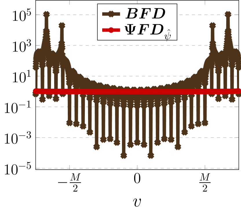
(a) $x\in\big{[}-\tfrac{1}{2},\tfrac{1}{2}\big{)}$

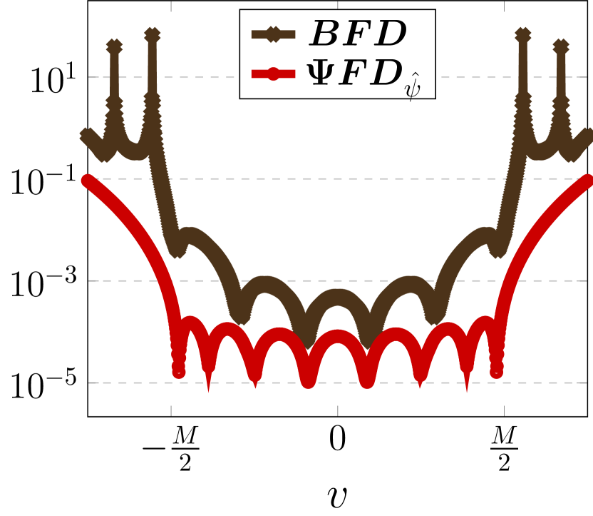
(b) $x\in\big{[}-\tfrac{1}{2}+\tfrac{m}{L},\tfrac{1}{2}-\tfrac{m}{L}\big{)}$

Figure 5.1: Maximum approximation error (5.3) for $P=10^{5}$ computed for (5.4) with $S=32$ using the $\sinh$-type window function (3.4) as well as the parameters $M=20$, $\lambda=1$, $L=(1+\lambda)M$, and $m=5$ in the one-dimensional setting $d=1$.

Example 5.1.

To examine the approximation quality of the NFFT-like procedure for bandlimited functions in Algorithm 4.1 we provide a function $f$ with its corresponding Fourier transform $\hat{f}$ in (3.1), such that we have access to the exact values $\hat{f}(k)$, $k\in\mathcal{I}_{M}$, as input for Algorithm 4.1, as well as the exact function evaluations $f(x_{j})$, $j=1,\dots,N$. In doing so, we can compare the result $f_{j}$, $j=1,\dots,N$, of Algorithm 4.1 to the exact function evaluations $f(x_{j})$, $j=1,\dots,N$, by computing the maximum approximation error

$$\max_{j=1,\dots,N}|f_{j}-f(x_{j})|.$$ (5.5)

For the reason of comparison, we also compute the approximation error (5.5) when $f_{j}$, $j=1,\dots,N$, is the result of the classical NFFT in Algorithm 2.1.

Here we consider the one-dimensional setting with $d=1$ and for several bandwidth parameters $M\in\{20,40,\dots,1000\}$ we study the function $f(x)=\mathrm{sinc}^{2}\big{(}\frac{M}{2}\pi x\big{)}$ with the Fourier transform

$$\hat{f}(v)=\frac{2}{M}\cdot\begin{cases}1-\big{|}\frac{2v}{M}\big{|}&\colon|v|\leq\frac{M}{2},\\ 0&\colon\text{otherwise}.\end{cases}$$

Note that the function $f$ is scaled appropriately such that $\max_{x\in\mathbb{R}}f(x)=1$ independent of the bandwidth $M$ and thereby the approximation errors (5.5) are comparable for all considered $M$. As evaluation points $x_{j}\in\big{[}-\frac{1}{2}+\frac{m}{L},\,\frac{1}{2}-\frac{m}{L}\big{]}$, $j=1,\dots,N$, we choose the scaled Chebyshev nodes

$$x_{j}=\cos\left(\frac{(j-1)\pi}{N}\right)\cdot\bigg{(}\frac{1}{2}-\frac{m}{L}\bigg{)},\quad j=1,\dots,N,$$ (5.6)

with $N=\frac{M}{2}$, $m=5$, as well as $M_{\sigma}=L=M(1+\lambda)$ with $\lambda=1$, and we use the $\sinh$-type window function (3.4).

The corresponding results are depicted in Figure 5.2. As expected by the previous comparison of the two approaches in Figure 5.1, the new NFFT-like procedure for bandlimited functions presented in Algorithm 4.1 performs much better than the classical NFFT in Algorithm 2.1. While for $M\leq 80$ both approaches exhibit the same maximum approximation error (5.5), for larger bandwidth $M$ the approximation error (5.5) gets smaller only for the NFFT-like procedure in Algorithm 4.1. That is to say, when approximating the evaluations $f(x_{j})$, $j=1,\dots,N$, of the bandlimited function $f\in\mathcal{B}_{M/2}(\mathbb{R})$ by given samples $\hat{f}(k)$, $k\in\mathcal{I}_{M}$, of the corresponding Fourier transform (3.1), reasonable results can be obtained by the NFFT in Algorithm 2.1, yet evidence indicates that our newly proposed NFFT-like procedure for bandlimited functions in Algorithm 4.1 yields results that are at least as good, if not superior. Accordingly, the NFFT-like procedure in Algorithm 4.1 is the preferred approach in this context.

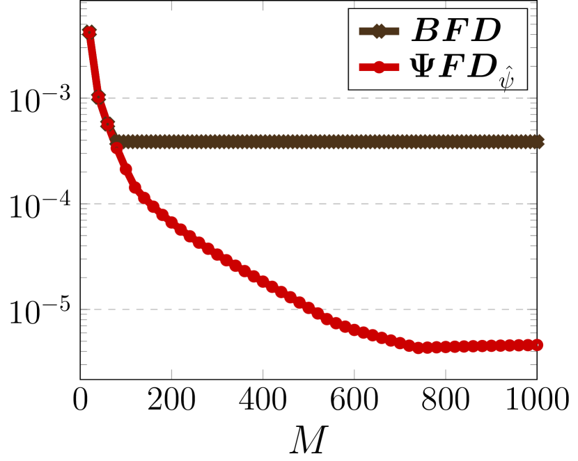
Figure 5.2: Maximum approximation error (5.5) of the NFFT-like procedure for bandlimited functions in Algorithm 4.1 and the classical NFFT in Algorithm 2.1 using the $\sinh$-type window function (3.4) computed for the function $f(x)=\mathrm{sinc}^{2}\big{(}\frac{M}{2}\pi x\big{)}$ using several bandwidth parameters $M\in\{20,40,\dots,1000\}$ and the scaled Chebyshev nodes (5.6) with $N=\frac{M}{2}$, $m=5$, $M_{\sigma}=L=(1+\lambda)M$, as well as $\lambda=1$ and $d=1$.

References

[1]
A. H. Barnett, J. F. Magland, and L. A. Klinteberg.
Flatiron Institute nonuniform fast Fourier transform libraries
(FINUFFT).
http://github.com/flatironinstitute/finufft.
[2]
G. Beylkin.
On the fast Fourier transform of functions with singularities.
Appl. Comput. Harmon. Anal., 2:363–381, 1995.
[3]
L. Chen and H. Zhang.
Sharp exponential bounds for the Gaussian regularized
Whittaker–Kotelnikov–Shannon sampling series.
J. Approx. Theory, 245:73–82, 2019.
[4]
I. Daubechies.
Ten Lectures on Wavelets.
SIAM, Philadelphia, PA, USA, 1992.
[5]
I. Daubechies and R. DeVore.
Approximating a bandlimited function using very coarsely quantized
data: A family of stable sigma-delta modulators of arbitrary order.
Ann. of Math., 158(2):679–710, 2003.
[6]
A. Dutt and V. Rokhlin.
Fast Fourier transforms for nonequispaced data.
SIAM J. Sci. Stat. Comput., 14:1368–1393, 1993.
[7]
H. G. Feichtinger.
New results on regular and irregular sampling based on Wiener
amalgams.
In K. Jarosz, editor, Function Spaces, Proc Conf,
Edwardsville/IL (USA) 1990, volume 136 of Lect. Notes Pure Appl. Math.,
pages 107––121. New York, 1992.
[8]
H. G. Feichtinger.
Wiener amalgams over Euclidean spaces and some of their
applications.
In K. Jarosz, editor, Function Spaces, Proc Conf,
Edwardsville/IL (USA) 1990, volume 136 of Lect. Notes Pure Appl. Math.,
pages 123––137. New York, 1992.
[9]
L. Greengard and J.-Y. Lee.
Accelerating the nonuniform fast Fourier transform.
SIAM Rev., 46:443–454, 2004.
[10]
D. Jagerman.
Bounds for truncation error of the sampling expansion.
SIAM J. Appl. Math., 14(4):714–723, 1966.
[11]
J. Keiner, S. Kunis, and D. Potts.
NFFT 3.5, C subroutine library.
http://www.tu-chemnitz.de/~potts/nfft.
Contributors: F. Bartel, M. Fenn, T. Görner, M. Kircheis, T. Knopp,
M. Quellmalz, M. Schmischke, T. Volkmer, A. Vollrath.
[12]
J. Keiner, S. Kunis, and D. Potts.
Using NFFT3 - a software library for various nonequispaced fast
Fourier transforms.
ACM Trans. Math. Software, 36:Article 19, 1–30, 2009.
[13]
M. Kircheis.
Fast Fourier Methods for Trigonometric Polynomials and
Bandlimited Functions.
Dissertation. Shaker Verlag, Düren, 2024.
[14]
M. Kircheis, D. Potts, and M. Tasche.
On regularized Shannon sampling formulas with localized sampling.
Sampl. Theory Signal Process. Data Anal., 20(20):34 pp., 2022.
[15]
M. Kircheis, D. Potts, and M. Tasche.
On numerical realizations of Shannon’s sampling theorem.
Sampl. Theory Signal Process. Data Anal., 22(13):33 pp., 2024.
[16]
V. A. Kotelnikov.
On the transmission capacity of the “ether” and wire in
electrocommunications.
In Modern Sampling Theory: Mathematics and Application, pages
27–45. Birkhäuser, Boston, 2001.
Translated from Russian.
[17]
R. Lin and H. Zhang.
Convergence analysis of the Gaussian regularized Shannon sampling
formula.
Numer. Funct. Anal. Optim., 38(2):224–247, 2017.
[18]
C. Micchelli, Y. Xu, and H. Zhang.
Optimal learning of bandlimited functions from localized sampling.
J. Complexity, 25(2):85–114, 2009.
[19]
F. Natterer.
Efficient evaluation of oversampled functions.
J. Comput. Appl. Math., 14(3):303–309, 1986.
[20]
J. R. Partington.
Interpolation, Identification, and Sampling.
Clarendon Press, London Mathematical Society Monographs New Series,
1997.
[21]
G. Plonka, D. Potts, G. Steidl, and M. Tasche.
Numerical Fourier Analysis.
Applied and Numerical Harmonic Analysis. Birkhäuser/Springer,
Second edition, 2023.
[22]
D. Potts and M. Tasche.
Uniform error estimates for nonequispaced fast Fourier transforms.
Sampl. Theory Signal Process. Data Anal., 19(17):1–42, 2021.
[23]
L. Qian.
On the regularized Whittaker–Kotelnikov–Shannon sampling formula.
Proc. Amer. Math. Soc., 131(4):1169–1176, 2003.
[24]
L. Qian.
The regularized Whittaker-Kotelnikov-Shannon sampling theorem
and its application to the numerical solutions of partial differential
equations.
PhD thesis, National Univ. Singapore, 2004.
[25]
T. S. Rappaport.
Wireless Communications: Principles and Practice.
Prentice Hall, New Jersey, 1996.
[26]
C. E. Shannon.
Communication in the presence of noise.
Proc. I.R.E., 37:10–21, 1949.
[27]
G. Steidl.
A note on fast Fourier transforms for nonequispaced grids.
Adv. Comput. Math., 9:337–353, 1998.
[28]
T. Strohmer and J. Tanner.
Fast reconstruction methods for bandlimited functions from periodic
nonuniform sampling.
SIAM J. Numer. Anal., 44(3):1071–1094, 2006.
[29]
E. T. Whittaker.
On the functions which are represented by the expansions of the
interpolation theory.
Proc. R. Soc. Edinb., 35:181–194, 1915.