Path optimization method for the sign problem caused by fermion determinant

Abstract

The path optimization method with machine learning is applied to the one-dimensional massive lattice Thirring model, which has the sign problem caused by the fermion determinant. This study aims to investigate how the path optimization method works for the sign problem. We show that the path optimization method successfully reduces statistical errors and reproduces the analytic results. We also examine an approximation of the Jacobian calculation in the learning process and show that it gives consistent results with those without an approximation.

I Introduction

To understand several important properties of quantum chromodynamics (QCD), such as the chiral phase transition and the confinement-deconfinement transition, the Markov chain Monte Carlo (MCMC) method is an important tool. In the MCMC calculation with the Boltzmann weight, expectation values are estimated using an ”effective action” for the probability distribution. However, the effective action can become complex at finite chemical potential even if the partition function itself is real. The weight can no longer be considered as a probability. Reweighting the imaginary part of the action is possible, but inefficient, especially for large volumes. This problem is called the sign problem; see Refs. de Forcrand (2009); Alexandru et al. (2022); Nagata (2020); *Nagata:2021ugx.

Since the partition function has an integral representation, we can address the sign problem by optimizing the integration path on the complexified dynamical variable plane with such as the path optimization method Mori et al. (2017, 2018) or the sign optimized manifold Alexandru et al. (2018a), which is related to the Lefschetz thimble method Witten (2011); Cristoforetti et al. (2012); Fujii et al. (2013) and the convex optimization Lawrence and Yamauchi (2024). The modification of the integration path does not change the integral as long as Cauchy’s integral theorem holds. The path optimization method has been applied to several models Mori et al. (2018); Kashiwa et al. (2019a); Bursa and Kroyter (2018); Kashiwa et al. (2019b); Mori et al. (2019); Kashiwa and Mori (2020); Namekawa et al. (2022, 2023); Giordano et al. (2022); Rodekamp et al. (2022, 2024); Kanwar et al. (2024); Lin et al. (2024), and measurement of observables Detmold et al. (2020, 2021); Bedaque and Oh (2024). In particular, the authors investigated the $0+1$ dimensional QCD in which the sign problem is induced by the quark determinant term Mori et al. (2019). It is important to extend the calculation to four-dimension, but the numerical cost is still very high. It motivates us to test the path optimization with machine learning for the one-dimensional Thirring model Thirring (1958) as a laboratory, which has the same origin of the sign problem as that of QCD. The Thirring model has been studied using the Lefschetz thimble method and its extensions Fujii et al. (2015a, b); Alexandru et al. (2016a, b); Fukuma and Umeda (2017); Di Renzo and Zambello (2022), the sign-optimized manifold approach Alexandru et al. (2018a, b), and the subtraction method Lawrence and Yamauchi (2023). It is an important check if the path optimization method using machine learning can reduce the sign problem as the other methods.

We also investigate a Jacobian approximation in the learning process for the lattice Thirring model. Since Jacobian calculation is dominant in the learning process, the cost reduction is highly desirable. It is important to evaluate efficiency of the Jacobian approximation for the model in which the sign problem occurs from the fermion determinant.

This paper is organized as follows. In Sec. II, we explain the formulation of the one-dimensional massive lattice Thirring model and the path optimization method. The numerical setup is shown in Sec. III. The numerical results are shown in Sec. IV, and Sec. V is devoted to the summary.

II Formulation

We employ the one-dimensional massive lattice Thirring model Pawlowski and Zielinski (2013); Fujii et al. (2015b) as a laboratory to investigate the sign problem caused by the fermion determinant term. First, we explain the formulation of the Thirring model. Next, we explain the application of the path optimization method with machine learning to the model.

II.1 One-dimensional massive Thirring model

The action of the one-dimensional lattice Thirring model with one flavor on a $L$ lattice is given by

$$S =S_{\mathrm{F}}+S_{\mathrm{B}},$$ (1)

where the fermion and boson parts are Pawlowski and Zielinski (2013); Fujii et al. (2015b),

$$S_{\mathrm{F}} =-\sum_{n=1}^{L}\bar{\chi}_{n}\Bigl{\{}e^{i\tilde{A}_{n}}\chi_{n+1}-e^{-i\tilde{A}_{n}}\chi_{n-1}+ma\chi_{n}\Bigr{\}},$$

$$S_{\mathrm{B}} =\beta\sum_{n=1}^{L}(1-\cos A_{n}),$$ (2)

here $\chi_{n}$ is fermion field at site $n$, $\tilde{A}_{n}$ denotes $A_{n}-i\mu a$, $A_{n}$ is a bosonic auxiliary field coupled to the vector current, $ma$ and $\mu a$ are the mass and chemical potential in the lattice unit $a$, respectively, and $\beta$ is the inverse coupling. To make the auxiliary field $A_{n}$ compact, the cosine function is introduced in $S_{\mathrm{B}}$ Fujii et al. (2015b). We set $a=1$ in all our calculations. We impose the antiperiodic boundary condition for the fermion field, and thus the system becomes thermal.

The partition function ${\cal Z}$ can be represented after integration of the fermion fields as

$${\cal Z}(\beta,\mu) =\int{\cal D}A{\cal D}\chi{\cal D}{\bar{\chi}}\,e^{-S}$$

$$=\int{\cal D}A\,e^{-\beta\sum_{n=1}^{L}(1-\cos A_{n})+\log\mathrm{det}\,D[A]},$$ (3)

where

$$D =\frac{1}{2^{L-1}}\Bigl{[}\cosh\Bigl{(}L\hat{\mu}+i\sum_{n=1}^{L}A_{n}\Bigr{)}+\cosh(L\hat{m})\Bigr{]},$$ (4)

here $\hat{m}=\sinh^{-1}(ma)$ and $\hat{\mu}=\mu a$. The field $A_{n}$ acts similarly to the gluon field in QCD, which leads to the appearance of the sign problem at finite $\mu\in\mathbb{R}$, although the structure is simpler. In the case of $\mu=0$, there is no sign problem.

Analytic results of the fermion condensate $s$ and the number density $n$ of the model are known Fujii et al. (2015b) as

$$s =\langle{\bar{\chi}}\chi\rangle$$

$$=\frac{I_{0}^{L}(\beta)\sinh(L\hat{m})}{I_{1}^{L}(\beta)\cosh(L\hat{\mu})+I_{0}^{L}(\beta)\cosh(L\hat{m})}\frac{1}{\cosh(\hat{m})},$$ (5)

and

$$n =-\frac{1}{L}\left\langle\frac{\partial S}{\partial\mu}\right\rangle$$

$$=\frac{I_{1}^{L}(\beta)\sinh(L\hat{\mu})}{I_{1}^{L}(\beta)\cosh(L\hat{\mu})+I_{0}^{L}(\beta)\cosh(L\hat{m})},$$ (6)

where $I_{k}(x)$ means the modified Bessel function of the first kind for $k=0,1$. Since we have the analytic result, we can estimate the correctness of the path optimization method for the sign problem induced by the fermion determinant term.

II.2 Path optimization method

In the path optimization method, the dynamical variables, $v\in\mathbb{R}$, are complexified as

$$v\mapsto v^{\prime}=v_{\mathrm{R}}+iv_{\mathrm{I}},$$ (7)

where $v_{\mathrm{R}},v_{\mathrm{I}}\in\mathbb{R}$. We employ the artificial neural network McCulloch and Pitts (1943); Hebb (2005); Rosenblatt (1958); Hinton and Salakhutdinov (2006) to represent the modified integral path as proposed in Ref. Mori et al. (2018):

$$\underbrace{v_{\mathrm{R}}}_{\mathrm{input\,layer}}\to\mathrm{hidden~layer}\to\underbrace{v_{\mathrm{I}}}_{\mathrm{output\,layer}}.$$ (8)

The output layer is

$$v_{\mathrm{I}l}=v^{(F)}_{l} =[w_{lk}^{(F-1)}f(v_{k}^{F-1})+b_{l}^{(F-1)}],$$ (9)

and the hidden layer is composed of

$$v_{k}^{(p+1)} =w_{kj}^{(p)}v_{j}^{(p)}+b_{k}^{(p)},$$ (10)

where

$$v^{(p)}_{j} =w_{ji}^{(p-1)}f(v_{i}^{(p-1)})+b_{j}^{(p-1)},$$ (11)

here $v^{(p)}$ means the quantities in the $p$-th hidden layer ($p=1,\cdots,F-1$) with $v^{(0)}=v_{\mathrm{R}}$, weight $W$ and bias $b$ are the parameters of the neural network. The function $f(\cdot)$ denotes the activation function, and we set $f(\cdot)=\tanh(\cdot)$.

To optimize the parameters of the neural network using the backpropagation method Rumelhart et al. (1986), we need the cost function ${\cal F}$. We use the following form

$${\cal F}[w,b] =\int dv_{\mathrm{R}}\,|e^{i\theta(v_{\mathrm{R}})}-e^{i\theta_{0}}|^{2}\,|J(v_{\mathrm{R}})\,e^{-S(v^{\prime})}|,$$ (12)

with $\theta=\arg(e^{-S+\ln J})$. $J(v_{\mathrm{R}})$ is Jacobian induced via the complexification, and $\theta_{0}$ means the phase of the partition function. In this study, $\theta_{0}=0$ is manifested since the partition function is definitely real. Based on the cost function, which reflects the seriousness of the sign problem, we can perform the training with configurations generated by using the Hybrid Monte Carlo (HMC) method Duane et al. (1987).

Even after obtaining a good modified integral path, the Boltzmann weight is still complex, and thus the reweighting method Ferrenberg and Swendsen (1988) is a possible choice. In this work, we use the phase reweighting as

$$\langle{\cal O}\rangle =\frac{\langle{\cal O}e^{i\theta}\rangle_{\mathrm{pq}}}{\langle e^{i\theta}\rangle_{\mathrm{pq}}},$$ (13)

where ${\cal O}$ represents observables and $\langle\cdots\rangle_{\mathrm{pq}}$ means the phase reweighted expectation values. The denominator of Eq. (13) is the so-called average phase factor (APF).

III Numerical setup

Our numerical codes are made using PyTorch Paszke et al. (2019). To evaluate the expectation values, we generate $1000$ configurations after thermalization using the HMC method. The statistical error is estimated using the Jackknife method with a bin size of $50$.

In the learning procedure, we employ AdamW Loshchilov and Hutter (2019), one of the stochastic gradient methods, as an optimizer. The number of units in the hidden layer is set to $64$. We use a single hidden layer $F=1$, which is found to reduce the sign problem sufficiently in our setup. Improvement of learning with the deep neural network is our future work. In the training part, we use batch training Bottou (1998) with the batch size of $64$.

After training, we regenerate the configurations and estimate the average phase factor and observables. This procedure is introduced to avoid the overtraining problem; we estimate the observables after the HMC update, not just after the training. If the average phase factor is not sufficiently enhanced in the early stage of the training, we consider that the initial values of the neural network parameters are not good and thus restart the calculation with different initial values of parameters.

IV Numerical results

We show our numerical results for the one-dimensional Thirring model mainly with the lattice size $L=16$. First, we show the full results, and later we argue an approximation of the Jacobian in the model.

Figure 1 shows the $\mu$-dependence of the fermion condensate (5) at $\beta=1$ and $2$ on the original and modified paths.

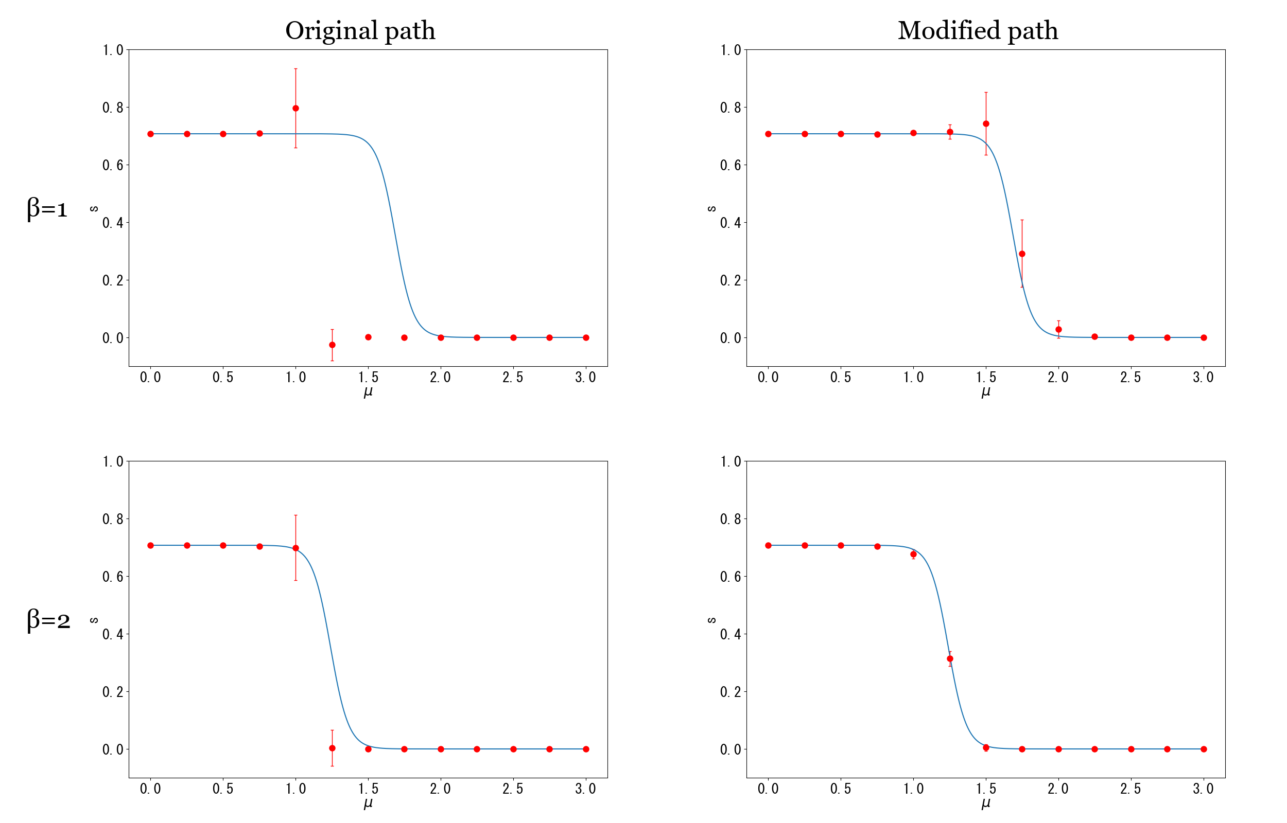
Figure 1: The $\mu$-dependence of the fermion condensate $s$ with $L=16$. The symbols are our numerical results, and the lines denote the analytic results. The left (right) panels are the results on the original (modified) path. The upper (lower) panels are the results at $\beta=1$ ($\beta=2$).

On the original path, the numerical results have huge errors due to the sign problem. In addition, at $\beta=1$, the numerical results do not reproduce the analytical results with small errors. This happens by an unbalanced sampling of configurations. It will be relaxed if we increase the number of configurations. On the modified integral path, we can reproduce the analytic results with small errors. Figure 2 shows the $\mu$-dependence of the number density (6) at $\beta=1$ and $2$.

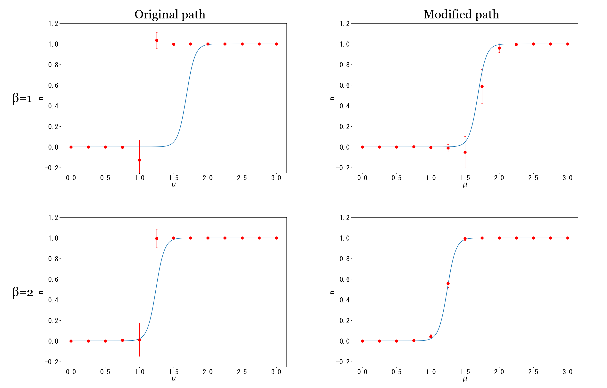
Figure 2: The $\mu$-dependence of the number density $n$ with $L=16$. The symbols are our numerical results, and the lines denote the analytic results. The left (right) panels are the results on the original (modified) path. The upper (lower) panels are the results at $\beta=1$ ($\beta=2$).

As in the case of the fermion condensate, our results on the modified path reproduce the analytic results with small errors, while those on the original path do not.

Figure 3 shows the $\mu$-dependence of the real part of APF at $\beta=1$ and $2$.

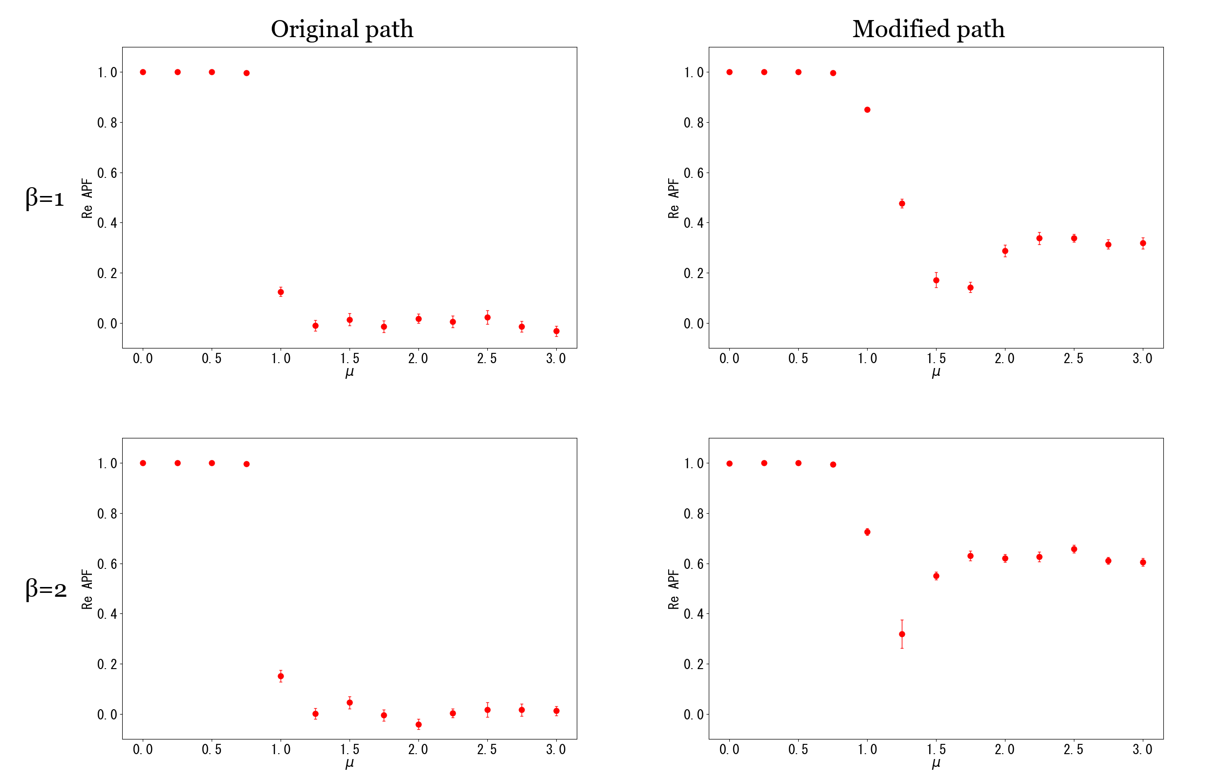
Figure 3: The $\mu$-dependence of the real part of APF with $L=16$. The left (right) panels are the results on the original (modified) path. The upper (lower) panels are the results at $\beta=1$ ($\beta=2$).

The path optimization enhances APF, which leads to better-controlled errors. It may be further improved by using a more complicated neural network because such a network has higher expressive power.

The deformation of the integral path is visualized by histograms of the phase of APF on the original and deformed integral paths. Below, we show histograms at $\beta=1$ as an example. The figures 4 and 5 represent the histograms of the phase at $\beta=1$. We can clearly see the difference between the histograms. At $\mu=0.25$ and $0.75$, the histogram is localized both on the original and modified paths, and AFP in Fig. 3 is close to one, indicating that the sign problem is mild. At larger $\mu$, the histogram on the original path shows almost flat dependence on $\theta$, and AFP is close to zero, indicating that the sign problem is severe. In contrast, the histogram on the modified path is still localized well, and AFP is non-zero, indicating that the sign problem is mild. It is noted that at $\mu=1.75$ we see a less clear peak in the histogram on the modified path. It suggests that several thimbles contribute to the result. As the Lefschetz thimble approach with parallel tempering (tempered Lefschetz thimble method) Fukuma and Umeda (2017) and its extension to the continuous accumulation of deformed surfaces (worldvolume HMC method) Fukuma and Matsumoto (2021); Fukuma et al. (2021); Fukuma (2024) successfully evaluated contribution from many thimbles, the path optimization combined with parallel tempering Kashiwa and Mori (2020) may further improve the result. This is our future work. Figures 6 and 7 exhibit histograms of $\mathrm{Re}\,\bar{\chi}\chi e^{i\theta}$ on the original and modified integral paths at $\beta=1$. At low and high $\mu$, the histograms are localized well both on the original and modified paths. At $\mu=1.25$ and $1.75$, on the other hand, the histograms are drastically changed by the path optimization, which leads to improvement of the signals.

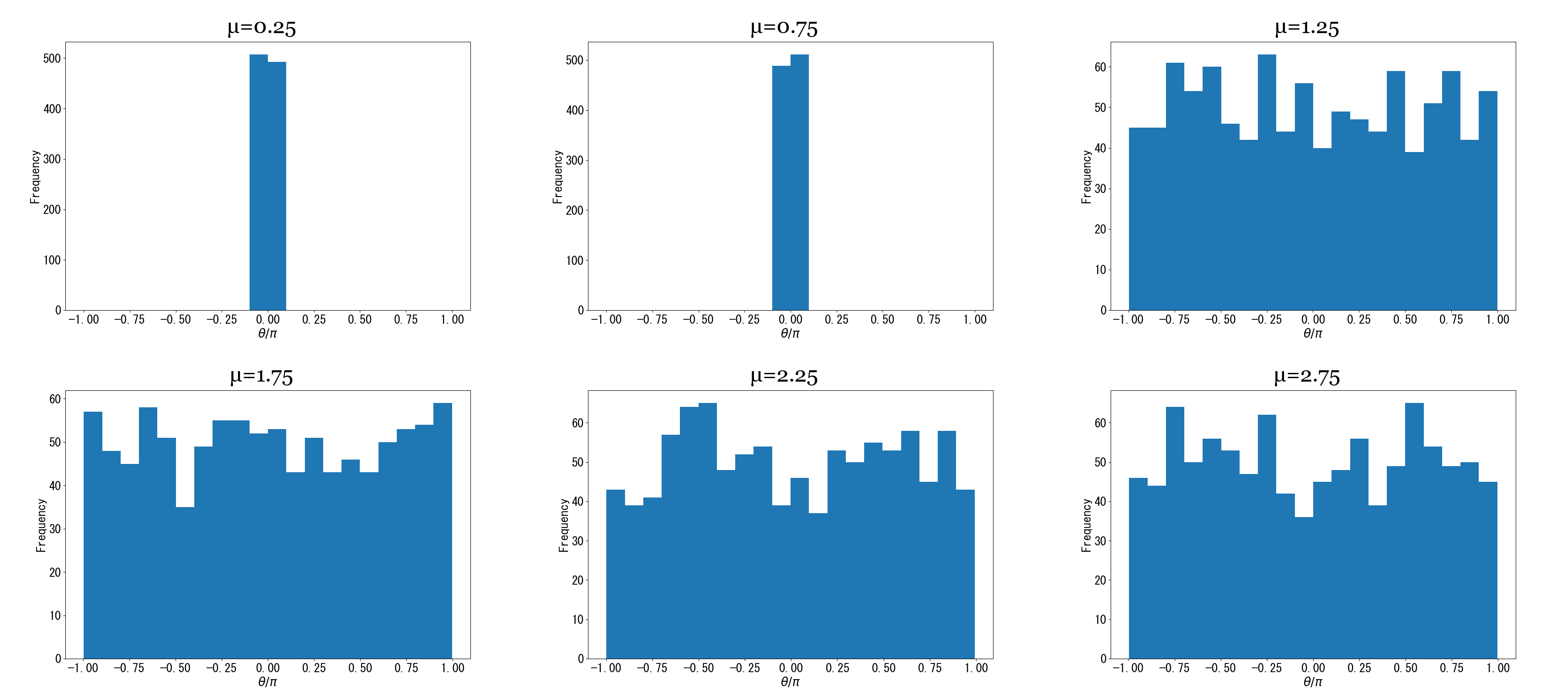
Figure 4: The histogram against $\theta$ on the original integral paths with $L=16$ at $\beta=1$. From the left-top to right-bottom panels, $\mu$ is set to $0.25$, $0.75$, $1.25$, $1.75$, $2.25$ and $2.75$.

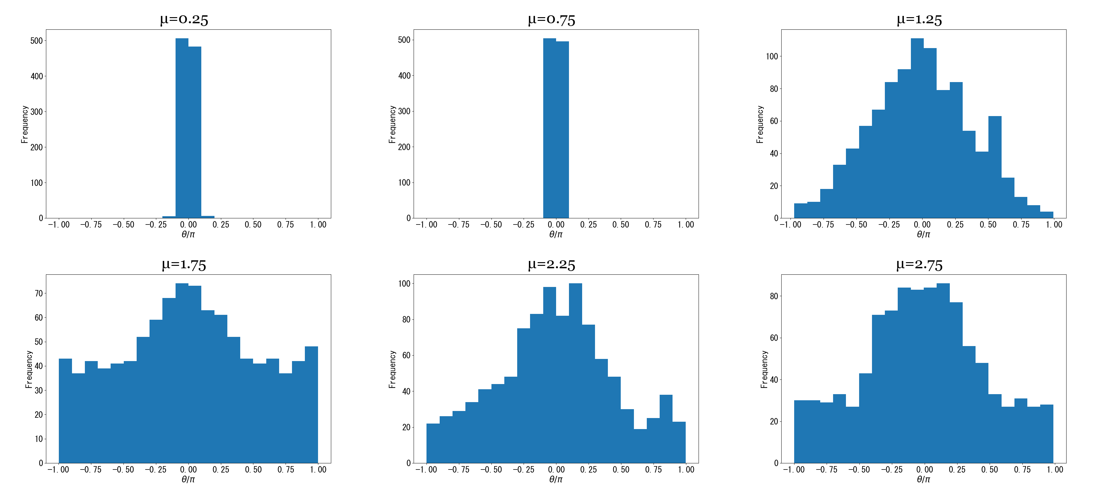
Figure 5: The histogram against $\theta$ on the modified integral paths with $L=16$ at $\beta=1$. From the left-top to right-bottom panels, $\mu$ is set to $0.25$, $0.75$, $1.25$, $1.75$, $2.25$ and $2.75$.

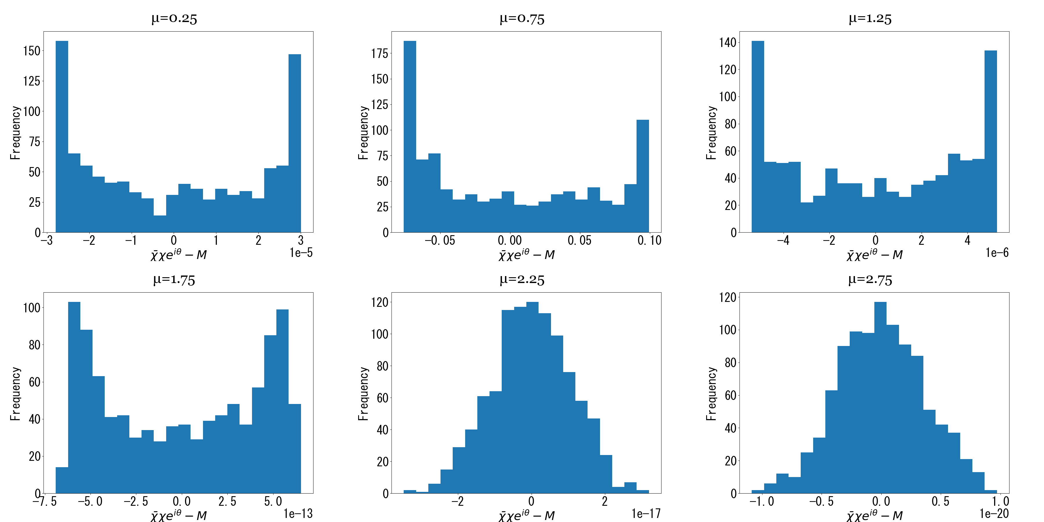
Figure 6: The histogram against $\mathrm{Re}\,\bar{\chi}\chi e^{i\theta}-M$ on the original integral paths with $L=16$ at $\beta=1$, where $M$ denotes the mean value of $\mathrm{Re}\,{\bar{\chi}}\chi e^{i\theta}$ at each $\mu$. From the left-top to right-bottom panels, $\mu$ is set to $0.25$, $0.75$, $1.25$, $1.75$, $2.25$ and $2.75$.

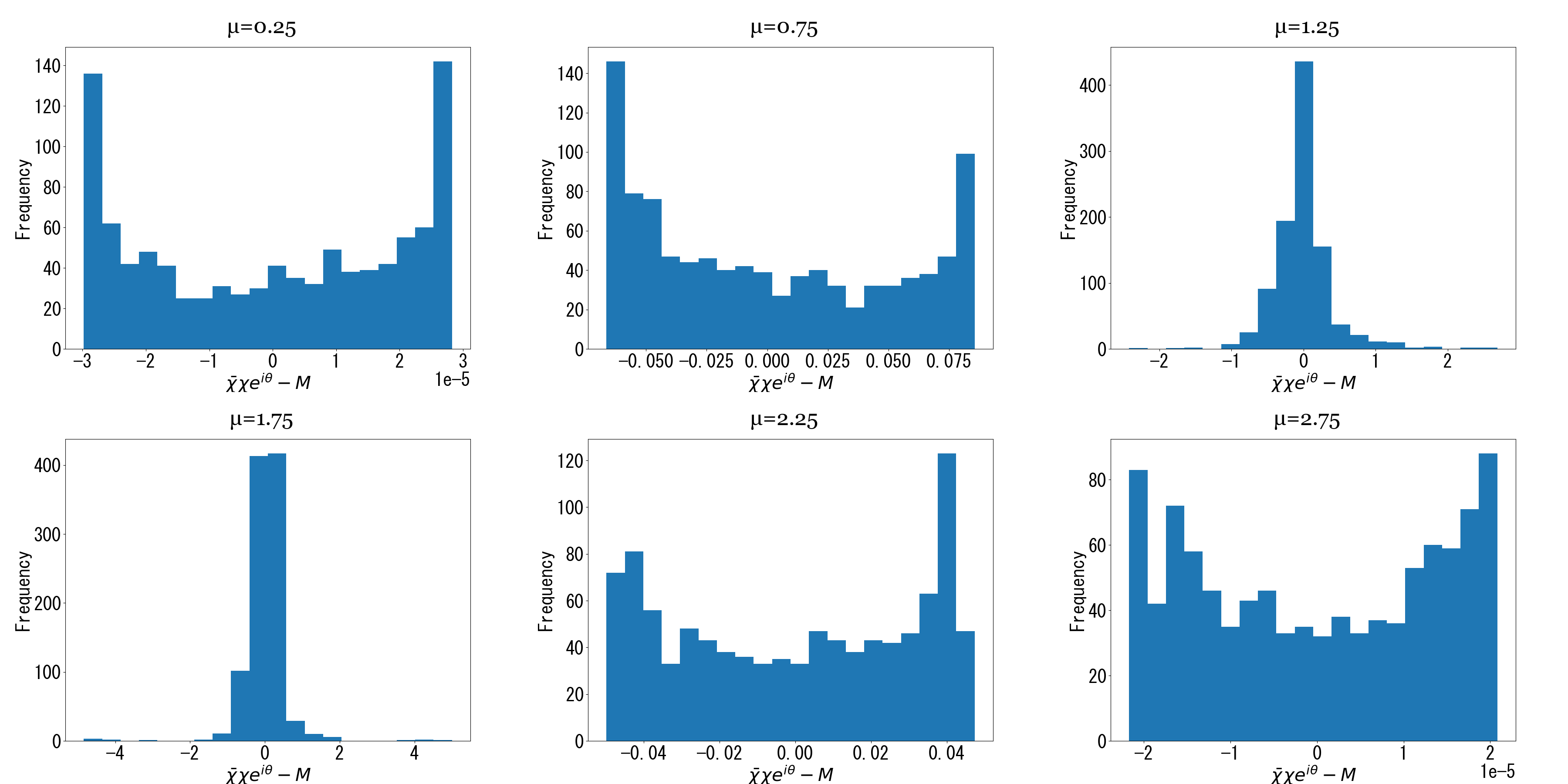
Figure 7: The histogram against $\mathrm{Re}\,\bar{\chi}\chi e^{i\theta}$ on the modified integral paths with $L=16$ at $\beta=1$, where $M$ denotes the mean value of $\mathrm{Re}\,{\bar{\chi}}\chi e^{i\theta}$ at each $\mu$. From the left-top to right-bottom panels, $\mu$ is set to $0.25$, $0.75$, $1.25$, $1.75$, $2.25$ and $2.75$.

The scaling behavior of APF at $\mu=1.0$ in terms of the system volume $L=4,8,16$ is shown in Fig. 8.

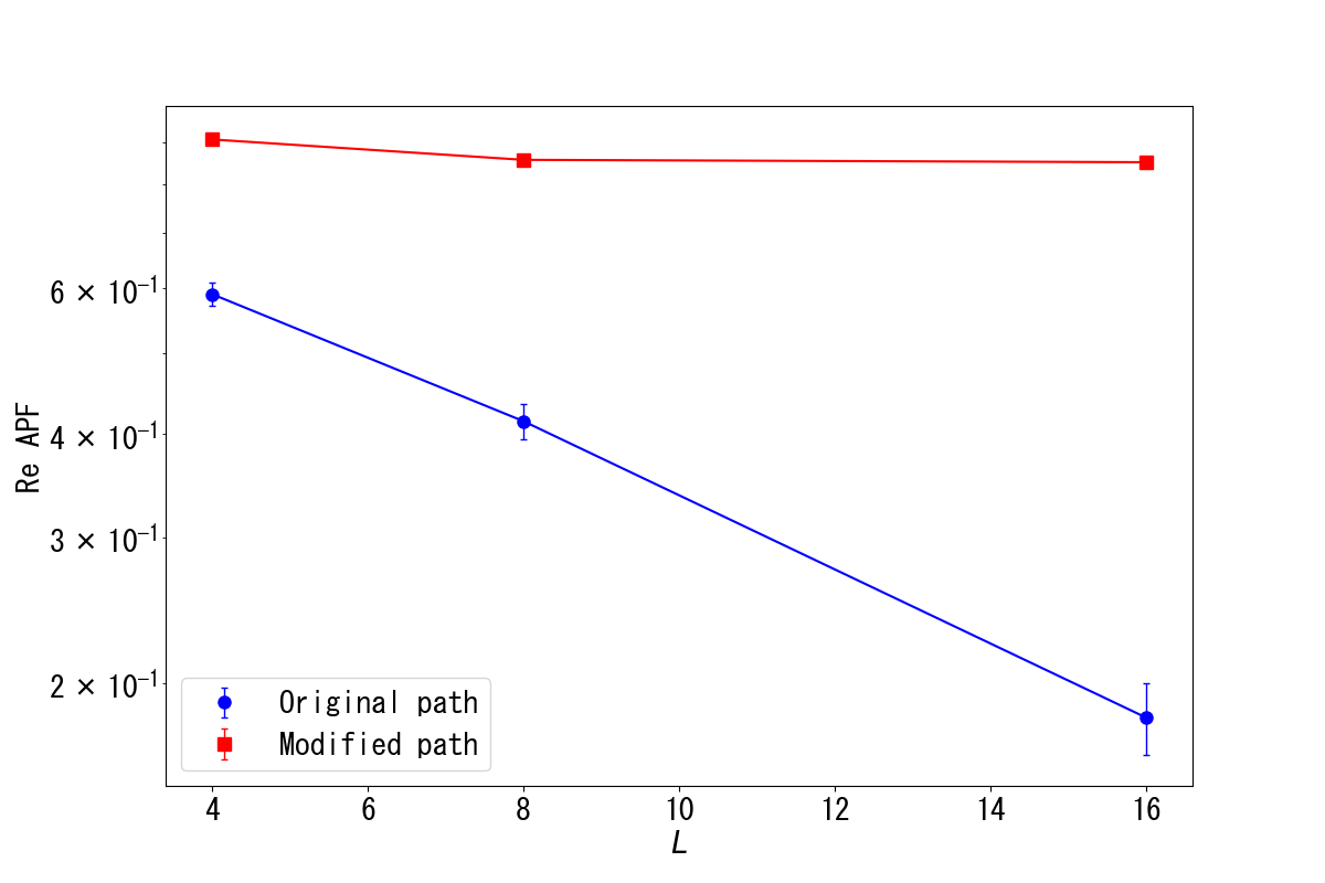
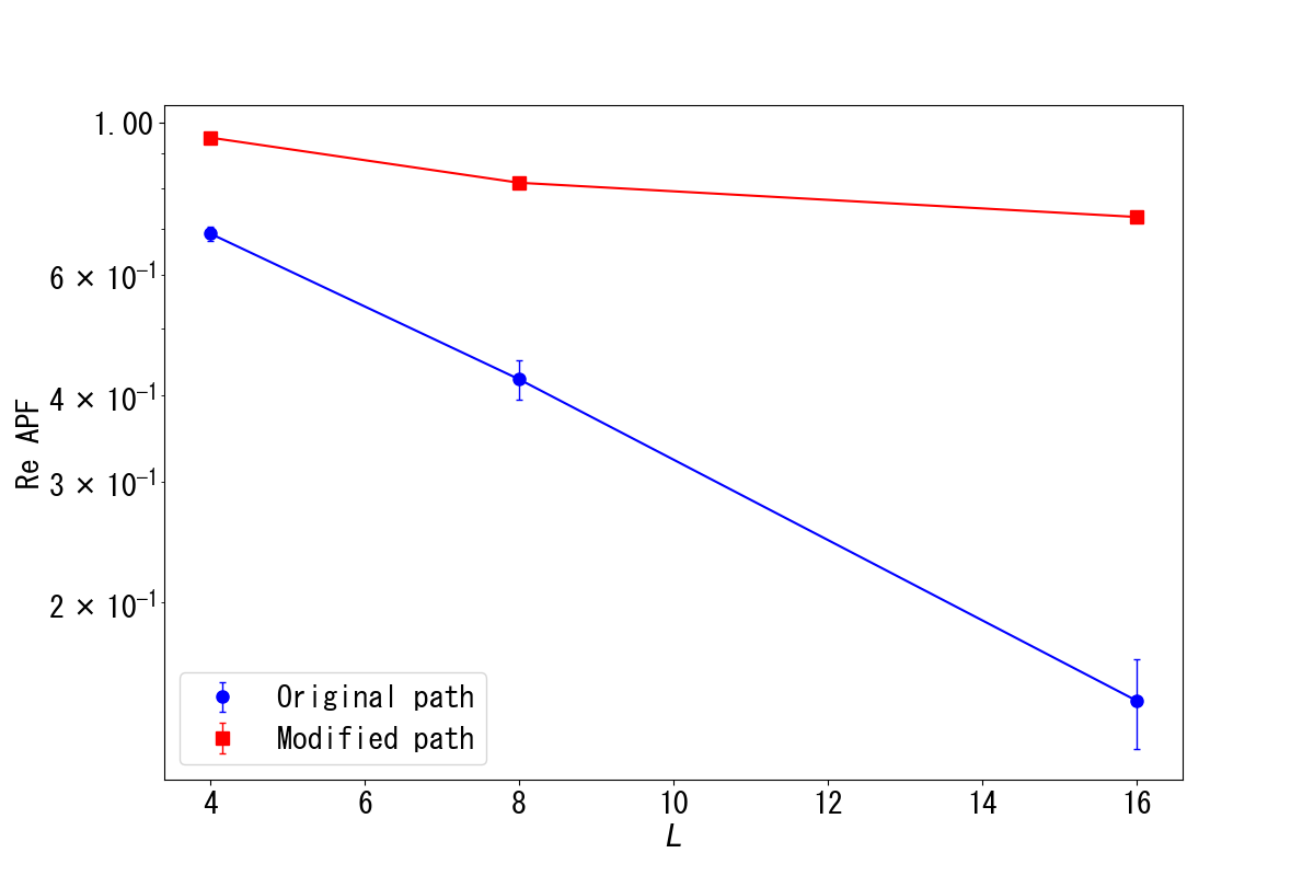
Figure 8: The upper (lower) panel shows the scaling behavior of APF with $\mu=1.0$ at $\beta=1$ ($\beta=2$). The circle and square symbols are the results on the original and modified integral paths, respectively.

We see a similar scaling law in both cases,

$$\mathrm{APF} \sim e^{-\alpha V},$$ (14)

where $\alpha$ is the $\phi$-dependent value; see Ref. Splittorff and Verbaarschot (2007) as an example. The modification of the integration path leads to a smaller value of $\alpha$, i.e., the path optimization successfully improves the scaling behavior. Of course, this method does not completely solve the curse of dimensionality.

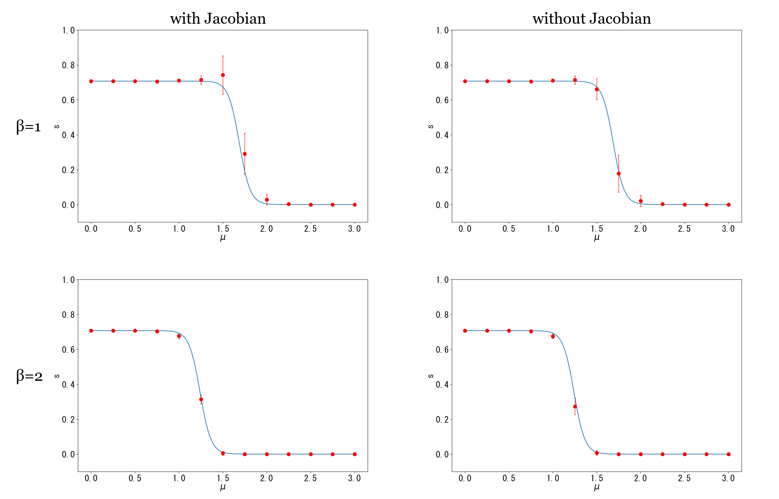
Figure 9: The $\mu$-dependence of the fermion condensate $s$ with $L=16$. The symbols are our numerical results with the Jacobian calculation (left) and without the Jacobian calculation (right) in the learning process, and the lines denote the analytic results. The upper (lower) panels are the results at $\beta=1$ ($\beta=2$).

Next, we consider the approximation of the Jacobian in the learning step for the Thirring model. The Jacobian calculation requires a large numerical cost ${\cal O}(N^{3})$, where $N$ is the total degrees of freedom. To reduce the cost, we employ the simplest approximation in which we replace the Jacobian matrix ${\cal J}$ with the unit matrix ${\mathbbm{1}}$ Namekawa et al. (2023);

$$J =\mathrm{det}\,{\cal J}\to\mathrm{det}\,\mathbbm{1}=1.$$ (15)

No numerical cost for the Jacobian calculation is required in the learning part. The Jacobian calculation is required only in the evaluation step of the observables. Figures 9 and 10 show the $\mu$-dependence of the fermion condensate and the number density at $\beta=1$ and $2$ with and without the Jacobian calculation in the learning process.

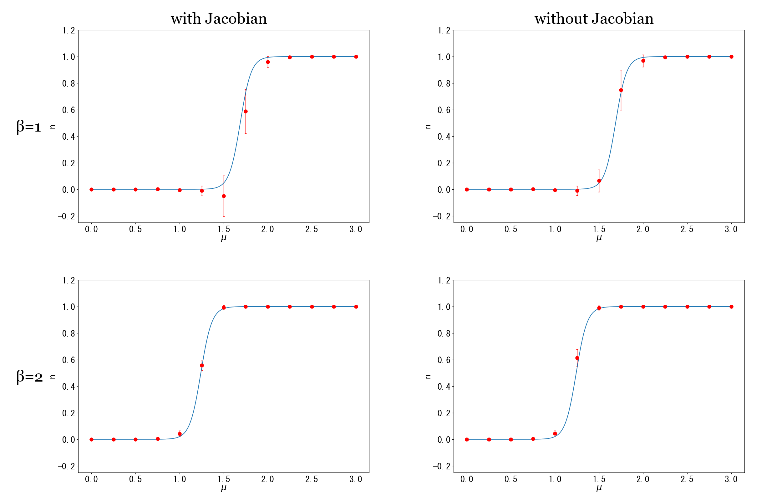
Figure 10: The $\mu$-dependence of the number density $n$ with $L=16$. The symbols are our numerical results with the Jacobian calculation (left) and without the Jacobian calculation (right) in the learning process, and the lines denote the analytic results. The upper (lower) panels are results at $\beta=1$ ($\beta=2$).

In both cases of $\beta$, the approximation of the Jacobian works. The results on the modified path reproduce the analytic values with comparable errors. Since the lattice Thirring model is similar to QCD in terms of the origin of the sign problem, our result suggests that the simplest approximation of the Jacobian in the learning step also works in QCD. Based on the above results, we can consider the following procedure; we first perform a few learning steps with the approximation of the Jacobian as a pre-training, and afterward, we perform the full learning. It is expected to be an efficient procedure with significant cost reduction, especially in the complicated theory/model.

V Summary

In this paper, we have applied the path optimization method with machine learning to the one-dimensional massive lattice Thirring model as a laboratory to investigate the sign problem via the fermion-determinant term. The modified integral path is represented by the neural network and the parameters are optimized via the self-supervise Learning-like method.

We found that the path optimization method with machine learning works well in the Thirring model. The average phase factor is enhanced on the modified integral path compared to the value on the original path, and our results agree with the analytic results with small statistical errors. It indicates that the path optimization method works for the sign problem from the fermion-determinant term, which is of the same origin as that in QCD.

The approximation of Jacobian in the lattice Thirring model has also been examined. We found that the perfect drop of the Jacobian calculation in the learning part, which significantly reduces the numerical cost, still works well. The calculations with and without the Jacobian approximation give consistent expectation values of observables with small errors.

Based on this success, we apply the path optimization method to a more QCD-like theory/model, where the fermion determinant causes the sign problem.