The alternative to Mahler measure of a multivariate polynomial

Dragan Stankov dstankov@rgf.bg.ac.rs Katedra Matematike RGF-a, Faculty of Mining and Geology, University of Belgrade, Belgrade, Đušina 7, Serbia dstankov@rgf.bg.ac.rs

Number theory

thanks: Partially supported by Serbian Ministry of Education and Science, Project 174032.

,

Abstract

We introduce the ratio of the number of roots of a polynomial $P_{d}$, less than one in modulus, to its degree $d$ as an alternative to Mahler measure. We investigate some properties of the alternative. We generalise this definition for a polynomial in several variables using Cauchy’s argument principle. If a polynomial in two variables do not vanish on the torus we prove the theorem for the alternative which is analogous to the Boyd-Lawton limit formula for Mahler measure. We determined the exact value of the alternative of $1+x+y$ and $1+x+y+z$. Numerical calculations suggest a conjecture about the exact value of the alternative of such polynomials having more than three variables.

1 Introduction

For a non-zero rational function $P\in\mathbb{C}(x_{1},\ldots,x_{k})$, we define the logarithmic Mahler measure of $P$ to be

$$m(P):=\int_{0}^{1}\int_{0}^{1}\cdots\int_{0}^{1}\log|P(e^{2\pi it_{1}},e^{2\pi it_{2}},\ldots,e^{2\pi it_{k}})|dt_{1}dt_{2}\cdots dt_{k}$$

It is the average value of $\log|P|$ over the unit $k-$torus. If

$$P(x)=a_{d}\prod_{j=1}^{d}(x-\alpha_{j})\in\mathbb{C}_{d}[x],$$ (1)

is a polynomial that has only one variable then Jensen’s formula implies

$$m(P)=\int_{0}^{1}\log|P(e^{2\pi it})|dt=\log|a_{d}|+\sum_{j:|\alpha_{j}|>1}\log|\alpha_{j}|.$$

Mahler measure of $P(x)$ is

$$M(P(x)):=\exp(m(P))=|a_{d}|\prod_{j=1}^{d}\max(1,|\alpha_{j}|).$$

Recall that a cyclotomic (circle dividing) polynomial is defined as an irreducible factor of $x^{n}-1$, $n\in\mathbb{N}$. Clearly, if $\Phi$ is cyclotomic, then $m(\Phi)=0$. A well known Kronecker’s Lemma states that $P\in\mathbb{Z}[x],P\neq 0,m(P)=0$ if and only if $P(x)=x^{n}\prod_{i}\Phi_{i}(x)$, where $\Phi_{i}(x)$ are cyclotomic polynomials. This also means that polynomials with integer coefficients have logarithmic Mahler measure greater than or equal to zero. In 1933 Lehmer asked a question which is still open: do we have a constant $\delta>0$ such that for any $P\in\mathbb{Z}[x]$ with non-zero logarithmic Mahler measure, we must also have $m(P)>\delta$? The smallest known logarithmic Mahler measure $>0$ of a polynomial with integer coefficients is:

$$m(x^{10}+x^{9}-x^{7}-x^{6}-x^{5}-x^{4}-x^{3}+x+1)\approx 0.162357612\ldots.$$

Properties of the logarithmic Mahler measure of a univariate polynomial:

(1) For $P\in Z[x]$, a non zero polynomial, it follows from Kronecker’s Lemma that $M(P)\geq 1$ which implies $m(P)\geq 0$.

(2) For $P,Q\in C[x]$, we have $m(P\cdot Q)=m(P)+m(Q)$, in particular for $c\in C\backslash\{0\}$, we have $m(cP)=\log|c|+m(P)$.

(3) For a cyclotomic polynomial denoted by $\Phi$, since $M(\Phi)=1$, we have $m(\Phi)=0$.

(4) Let P be the product of cyclotomic polynomials, then, we have $m(P)=0$, and in addition, for any $n\in N$ we have $m(\pm x^{n}P)=0$ .

In general, calculating the Mahler measure of multi-variable polynomials is much more difficult than the univariate case. We have the Boyd-Lawton formula for any rational function $P\in\mathbb{C}(x_{1},\ldots,x_{k})$

$$\lim_{n_{2}\to\infty}\cdots\lim_{n_{k}\to\infty}m(P(x,x^{n_{2}},\ldots,x^{n_{k}}))=m(P(x_{1},x_{2},\ldots,x_{k})),$$

where the $n_{j}$’s vary independently.

It turns out that for certain polynomials, the Mahler measure is in fact a special value of an $L-$function. In 1981 Smyth proved that

$$m(1+x+y)=\frac{3\sqrt{3}}{2\pi}L(\chi_{-3},2)=L^{\prime}(\chi_{-3},-1),$$ (2)
$$m(1+x+y+z)=\frac{7}{2\pi^{2}}\zeta(3)=-14\zeta^{\prime}(-2).$$ (3)

Pritsker [17] defined a natural areal analog of the Mahler measure and studied its properties. Flammang [10] introduced the absolute S-measure for polynomial (1) defined by

$$s(P):=\frac{1}{d}\sum_{j=1}^{d}|{\alpha}_{j}|,$$

as an analog to Mahler measure and studied its properties. For many sequences of polynomials we calculated [18] the limit ratio of the number of roots out of the unit circle to its degree. Each sequence is correlated to a bivariate polynomial having small Mahler measure discovered by Boyd and Mossinghoff [4].

We introduce $c(P)$, our alternative to Mahler measure of a polynomial $P$, as the probability that a randomly chosen zero of $P$ is less than 1 in modulus. At the beginning of second section of [17] normalized zero counting measure for polynomial (1) is defined by

$$\nu_{d}:=\frac{1}{d}\sum_{j=1}^{d}\delta_{{\alpha}_{j}},$$

where $\delta_{{\alpha}_{j}}$ is the unit pointmass at ${\alpha}_{j}$. We can see that $c(P)=\nu_{d}$ of the open unit disc.

We generalise the definition of $c$ for bivariate polynomials and prove

Theorem 1.1
$$c(a+x+y)=\frac{\arccos(|a|/2)}{\pi}$$

The obvious consequence of Theorem 1.1 is:

Corollary 1.2
$$c(1+x+y)=\frac{1}{3}.$$

We generalise the definition of $c$ for multivariate polynomials and prove

Theorem 1.3
$$c(1+x+y+z)=\frac{1}{4}.$$

We show that the Boyd-Lawton formula is also valid for our alternative to Mahler measure of a multivariate polynomial $P$ and prove its consequence:

Corollary 1.4
$$\lim_{n_{2}\to\infty}\lim_{n_{3}\to\infty}c(1+x+x^{n_{2}}+x^{n_{3}})=\frac{1}{2},$$

where the $n_{j}$’s vary independently.

2 The alternative to Mahler measure of a bivariate polynomial

Theorem 2.1

(Cauchy’s argument principle) If $f(x)$ is a meromorphic function inside and on some closed, simple contour $C$, and $f$ has no zeros or poles on $C$, then

$$\frac{1}{2\pi i}\oint_{C}\frac{f^{\prime}(x)}{f(x)}dx=Z-\Pi$$

where $Z$ and $\Pi$ denote respectively the number of zeros and poles of $f(x)$ inside the contour $C$, with each zero and pole counted as many times as its multiplicity and order, respectively, indicate.

If $f(x)$ is a polynomial $P(x)$ of degree $d$ and $C$ is the unit circle then we set $x=e^{2\pi it}$, $dz=2\pi ie^{2\pi it}$ probability that a randomly chosen zero is inside the unit circle is

$$c(P):=\frac{1}{d}\int_{0}^{1}\frac{P^{\prime}(e^{2\pi it})e^{2\pi it}}{P(e^{2\pi it})}dt=\frac{Z}{d}$$

Properties of the alternative Mahler measure of univariate polynomials:

(1) For $P\in C[x]$, we have $0\leq c(P)\leq 1$.

(2) For $P\in Z[x]$, a non zero polynomial, it follows from Kronecker’s Lemma that $c(P)<1$.

(3) If $P(x)=a_{d}x^{d}+a_{d-1}x^{d-1}+a_{0}$ and $a_{0}\neq 0$ then for the reciprocal polynomial $P^{*}$ defined $P^{*}(x)=x^{d}P(1/x)$ we have

$$c(P^{*})=1-c(P).$$ (4)

(4) For $P,Q\in C[x]$, we have $(\deg(P)+\deg(Q))c(P\cdot Q)=\deg(P)c(P)+\deg(Q)c(Q)$, in particular for $\alpha\in C\backslash\{0\}$, we have $c(\alpha P)=c(P)$.

Before presenting the following definition, we need to provide an explanation. For a two variable polynomial $P(x,y)$ as in Boyd-Lawton formula we want to determine the limit of the probability $c(P(x,x^{n}))$ when $n\to\infty$.

Let $P(x,y)$ can be written

$$P(x,y)=a_{g}(x)y^{g}+a_{g-1}(x)y^{g-1}+\cdots+a_{0}(x).$$

The degree $d$ of $P(x,x^{n})$ is

$$d=\deg(a_{g}(x))+ng.$$ (5)
$$c(P(x,x^{n}))=\frac{1}{d}\int_{0}^{1}\frac{\frac{\partial}{\partial x}P(e^{2\pi it},e^{2\pi int})e^{2\pi it}+n\frac{\partial}{\partial y}P(e^{2\pi it},e^{2\pi int})e^{2\pi int}}{P(e^{2\pi it},e^{2\pi int})}dt.$$

We can split the previous integral into two integrals and replace $d$ using (5). The first integral

$$\frac{1}{\deg(a_{g}(x))+ng}\int_{0}^{1}\frac{\frac{\partial}{\partial x}P(e^{2\pi it},e^{2\pi int})e^{2\pi it}}{P(e^{2\pi it},e^{2\pi int})}dt\to 0,\;\;n\to\infty.$$

The second integral

$$\frac{1}{\deg(a_{g}(x))+ng}\int_{0}^{1}\frac{n\frac{\partial}{\partial y}P(e^{2\pi it},e^{2\pi int})e^{2\pi int}}{P(e^{2\pi it},e^{2\pi int})}dt\to\frac{1}{g}\int_{0}^{1}\frac{\frac{\partial}{\partial y}P(e^{2\pi it},e^{2\pi int})e^{2\pi int}}{P(e^{2\pi it},e^{2\pi int})}dt,$$

as $n$ tends to infinity. The term $e^{2\pi it}$ becomes increasingly uncorrelated with $e^{2\pi int}$ as $n\to\infty$, so that $nt$ can be replaced with a variable $s$ that vary independently to $t$:

$$\lim_{n\to\infty}\frac{1}{g}\int_{0}^{1}\frac{\frac{\partial}{\partial y}P(e^{2\pi it},e^{2\pi int})e^{2\pi int}}{P(e^{2\pi it},e^{2\pi int})}dt=\frac{1}{g}\int_{0}^{1}\int_{0}^{1}\frac{\frac{\partial}{\partial y}P(e^{2\pi it},e^{2\pi is})e^{2\pi is}}{P(e^{2\pi it},e^{2\pi is})}dtds.$$

It is now clear why we introduce the following

Definition 2.2

The alternative Mahler measure for a bivariate polynomial $P(x,y)$, having no zeros on the unit torus, is

$$c(P(x,y)):=\frac{1}{g}\int_{0}^{1}\int_{0}^{1}\frac{\frac{\partial}{\partial y}P(e^{2\pi it},e^{2\pi is})e^{2\pi is}}{P(e^{2\pi it},e^{2\pi is})}dtds.$$

Everest and Ward in [9] proved their Lemma 3.22 using the Stone-Weierstrass theorem. We present here the lemma as

Lemma 2.3

Let $\phi:K^{2}\rightarrow\mathbb{C}$ be any continuous function. Then

$$\lim_{n\to\infty}\int_{0}^{1}\phi(e^{2\pi it},e^{2\pi int})dt=\int_{0}^{1}\int_{0}^{1}\phi(e^{2\pi it},e^{2\pi is})dt\;ds.$$

We can prove now that the Boyd-Lawton formula is also valid for our alternative $c$ to Mahler measure.

Corollary 2.4

If a polynomial $P(x,y)$ does not vanish on the unit torus then

$$\lim_{n\to\infty}c(P(x,x^{n}))=c(P(x,y)).$$
{@proof}

[Proof] We have to prove that

$$\lim_{n\to\infty}\frac{1}{g}\int_{0}^{1}\frac{\frac{\partial}{\partial y}P(e^{2\pi it},e^{2\pi int})e^{2\pi int}}{P(e^{2\pi it},e^{2\pi int})}dt=\frac{1}{g}\int_{0}^{1}\int_{0}^{1}\frac{\frac{\partial}{\partial y}P(e^{2\pi it},e^{2\pi is})e^{2\pi is}}{P(e^{2\pi it},e^{2\pi is})}dtds.$$

Since the integrand is a continuous function it follows that we can use Lemma 2.3. ∎

In our previous paper [19] we determined the limit ratio between number of roots outside the unit circle of

$$P_{n}(x)=x^{n}+ax+1$$

and its degree $n$.

Theorem 2.5

The rate $\frac{\nu_{n,a}}{n}$ between the number $\nu_{n,a}$ of roots of the trinomial $x^{n}+ax+1$, $a\in(0,2]$, which are greater than 1 in modulus, and degree $n$, tends to $\frac{1}{\pi}\arccos(-\frac{a}{2})$, $n\to\infty$.

As $P_{n}(x)=x^{n}+ax+1=P(x,x^{n})$ where $P(x,y)=y+ax+1$ we can use our double integral formula. We can verify that these two values

$$1-\frac{1}{\pi}\arccos(-\frac{a}{2}),$$
$$\int_{0}^{1}\int_{0}^{1}\frac{e^{2\pi is}}{e^{2\pi is}+ae^{2\pi it}+1}dtds$$

match to a few decimal places depending of the precision of the definite integral calculator.

Lemma 2.6

If $|a|\neq 1$ then

$$\int_{0}^{1}\frac{e^{2\pi it}}{e^{2\pi it}+a}dt=\left\{\begin{array}[]{ll}0&\mbox{if }|a|>1\\ 1&\mbox{if }|a|<1\end{array}\right.=:1_{D}(a)$$
{@proof}

[Proof] It is the direct consequence of Cauchy’s argument principle. ∎

Lemma 2.7

If $s\in\left[-\frac{1}{3},\frac{1}{3}\right]$ then $|1+e^{2\pi is}|>1$

{@proof}

[Proof] We use the fact that

$$|1+e^{2\pi is}|=2\cos(\pi s).$$ (6)

{@proof}

[Proof] of Theorem 1.1 
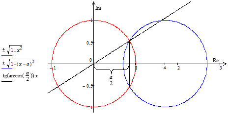
It is convenient to use the obvious fact that c(a+x+y)=cx(a+x+y)c(a+x+y)=c_{x}(a+x+y). If we: 1. use the definition of cx(P(x,y))c_{x}(P(x,y)), 2. use Lemma 2.6, 3. change the variable 2πs=φ2\pi s=\varphi in the definite integral, 4. use the determination of φ\varphi presented on the Figure 1., 5. calculate the definite integral, we obtain the following five steps:

$\displaystyle c(a+x+y)$ $\displaystyle=\int_{0}^{1}\int_{0}^{1}\frac{e^{2\pi it}}{e^{2\pi it}+e^{2\pi is}+a}dtds$
$\displaystyle=\int_{0}^{1}1_{D}(e^{2\pi is}+a)ds$
$\displaystyle=\frac{1}{2\pi}\int_{0}^{2\pi}1_{D}(e^{\varphi i}+a)d\varphi$
$\displaystyle=\frac{1}{2\pi}\int_{\pi-\arccos(|a|/2)}^{\pi+\arccos(|a|/2)}1\cdot d\varphi$
$\displaystyle=\frac{\arccos(|a|/2)}{\pi}.$

∎ We present Smyth’s proof [15, 5] of (2) to illustrate that there is an analogy with our proof of the Theorem 1.1. {@proof}[Proof] (Smyth 1981) of (2). We use Jensen’s formula: $\int_{0}^{1}\log|1+x+e^{2\pi is}|ds=\log^{+}|1+x|)$

$$m(1+x+y)=\int_{-1/2}^{1/2}\log^{+}|1+e^{2\pi it}|dt=\int_{-1/3}^{1/3}\log|1+e^{2\pi it}|dt$$
$$\Re\int_{-1/3}^{1/3}\log(1+e^{2\pi it})dt=\Re\int_{-1/3}^{1/3}\sum_{n=1}^{\infty}\frac{(-1)^{n-1}e^{2\pi int}}{n}dt$$
$$=\Re\left.\sum_{n=1}^{\infty}\frac{(-1)^{n-1}e^{2\pi int}}{2\pi in^{2}}\right|_{t=-1/3}^{t=1/3}=\frac{1}{\pi}\sum_{n=1}^{\infty}\frac{(-1)^{n-1}\sin\frac{2\pi n}{3}}{n^{2}}$$

It remains to use $\sin\frac{2\pi n}{3}=\chi_{-3}(n)$ and the multiplicativity of the character $\chi_{-3}$. ∎

Refer to caption
Figure 1: The determination of $\varphi$ such that $e^{\varphi i}+a$ (it is located on the blue circle) is inside of the unit circle (the red circle). It follows that $\varphi\in[\pi-\arccos(|a|/2),\pi+\arccos(|a|/2)]$.

We can show by changing the order of integration in a double integral that switching of the variables in a bivariate polynomial does not effect to the Mahler measure i.e. $m(P(x,y))=m(P(y,x))$. For the alternative to Mahler measure this is not true. We can demonstrate this with the following

Example 1

If $P(x,y)=xy+x+1$ we can show that $c(P(x,y))\neq c(P(y,x))$:

$\displaystyle c(xy+x+1)$ $\displaystyle=\lim_{x\to\infty}c(x^{n+1}+x+1)$
$\displaystyle=1/3,$

using Corollary 1.2. On the other hand if we switch the variables and determine $c(P(y,x))$ using Boyd-Lawton formula for $c$ and property (4) we obtain

$\displaystyle c(yx+y+1)$ $\displaystyle=\lim_{n\to\infty}c(x^{n+1}+x^{n}+1)$
$\displaystyle=\lim_{n\to\infty}c(x^{n+1}(1+\frac{1}{x}+\frac{1}{x^{n+1}}))$
$\displaystyle=\lim_{n\to\infty}c((1+x+x^{n+1})^{*})$
$\displaystyle=\lim_{n\to\infty}(1-c(x^{n+1}+x+1))$
$\displaystyle=1-c(xy+x+1)$
$\displaystyle=1-1/3$
$\displaystyle=2/3.$

3 The alternative to Mahler measure of a multivariate polynomial

Let $P(x_{1},x_{2},\ldots,x_{k})$ can be written

$$P(x_{1},x_{2},\ldots,x_{k})=a_{d_{j}}(x_{1},\ldots,x_{j-1},x_{j+1},\ldots,x_{k})x_{j}^{d_{j}}+$$
$$+a_{d_{j}-1}(x_{1},\ldots,x_{j-1},x_{j+1},\ldots,x_{k})x_{j}^{d_{j}-1}+\cdots+a_{0}(x_{1},\ldots,x_{j-1},x_{j+1},\ldots,x_{k}).$$
Definition 3.1

The alternative measure $c_{x_{j}}$, with respect to $x_{j}$, or abbreviated $c_{j}$ for a polynomial in $k$ variables $P(x_{1},x_{2},\ldots,x_{k})$, having no zeros on the unit $k$-torus, is

$$c_{j}(P(x_{1},x_{2},\ldots,x_{k})):=\frac{1}{d_{j}}\int_{0}^{1}\int_{0}^{1}\cdots\int_{0}^{1}\frac{\frac{\partial}{\partial x_{j}}P(e^{2\pi it_{1}},e^{2\pi it_{2}},\ldots,e^{2\pi it_{k}})e^{2\pi it_{j}}}{P(e^{2\pi it_{1}},e^{2\pi it_{2}},\ldots,e^{2\pi it_{k}})}dt_{1}dt_{2}\cdots dt_{k}.$$
Remark 1

If we use $c$ without a subscript it means that the last variable of $P$ should be taken as the subscript so that $c(P(x_{1},x_{2},\ldots,x_{k}))=c_{k}(P(x_{1},x_{2},\ldots,x_{k}))$ and $c(P(x,y,z))=c_{z}(P(x,y,z))$.

In the previous example we showed that $c(P(x,y))=c_{y}(P(x,y))=1/3$ and $c(P(y,x))=c_{y}(P(y,x))=c_{x}(P(x,y))=2/3$ so that $c_{x}(P(x,y))\neq c_{y}(P(x,y)).$

{@proof}

[Proof] of Theorem 1.3. Again it is convenient to use the obvious fact that $c(1+x+y+z)=c_{x}(1+x+y+z)$ 1. If we use: the definition of $c_{x}(1+x+y+z)$, 2. Theorem 1.1 taking $a=e^{2\pi iu}+1$, 3. Equation (6), 4. the fact that $\arccos\cos(\pi u)=\pi u$, $u\in[0,1/2]$, 5. the calculation of the definite integral, we obtain the following five steps:

$\displaystyle c(1+x+y+z)$ $\displaystyle=\int_{0}^{1}\int_{0}^{1}\int_{0}^{1}\frac{e^{2\pi it}}{e^{2\pi it}+e^{2\pi is}+e^{2\pi iu}+1}dtdsdu$
$\displaystyle=\int_{0}^{1}\frac{\arccos(|e^{2\pi iu}+1|/2)}{\pi}du$
$\displaystyle=2\int_{0}^{1/2}\frac{\arccos\cos(\pi u)}{\pi}du$
$\displaystyle=2\int_{0}^{1/2}\frac{\pi u}{\pi}du$
$\displaystyle=\frac{1}{4}.$

Numerical calculations of multiple integrals of such functions of $k\leq 6$ variables

$$c_{k}(1+x_{1}+x_{2}+\ldots+x_{k})):=\int_{0}^{1}\int_{0}^{1}\cdots\int_{0}^{1}\frac{e^{2\pi it_{k}}}{1+e^{2\pi it_{1}}+e^{2\pi it_{2}}+\ldots+e^{2\pi it_{k}}}dt_{1}dt_{2}\cdots dt_{k}.$$

suggest us that the following conjecture is valid:

Conjecture 3.1
$$c(1+x_{1}+x_{2}+\cdots+x_{k})=\frac{1}{k+1}.$$
Theorem 3.2

If $P(x_{1},x_{2},\ldots,x_{k})$ does not vanish on the torus $T^{k}$ then

$$\lim_{n_{2}\to\infty}\cdots\lim_{n_{k}\to\infty}c(P(x_{1},x_{1}^{n_{2}},\ldots,x_{1}^{n_{k}}))=c_{2}(P(x_{1},x_{2},\ldots,x_{k}))+\cdots+c_{k}(P(x_{1},x_{2},\ldots,x_{k})).$$
{@proof}

[Proof] Let $P(x_{1},x_{2},\ldots,x_{k})$ can be written

$$P(x_{1},x_{2},\ldots,x_{k})=a_{j,d_{j}}(x_{1},\ldots,x_{j-1},x_{j+1},\ldots,x_{k})x_{j}^{d_{j}}+$$
$$+a_{j,d_{j}-1}(x_{1},\ldots,x_{j-1},x_{j+1},\ldots,x_{k})x_{j}^{d_{j}-1}+\cdots+a_{j,0}(x_{1},\ldots,x_{j-1},x_{j+1},\ldots,x_{k}),\;\;j=2,\ldots,k.$$

The degree $d$ of $P(x_{1},x_{1}^{n_{2}},\ldots,x_{1}^{n_{k}})$ is

$$d=\deg(a_{j,d_{j}}(x_{1},\ldots,x_{1}^{n_{j-1}},x_{1}^{n_{j+1}},\ldots,x_{1}^{n_{k}}))+n_{j}d_{j}.$$ (7)
$$c(P(x_{1},x_{1}^{n_{2}},\ldots,x_{1}^{n_{k}}))=$$
$$=\frac{1}{d}\int_{0}^{1}\frac{\frac{\partial}{\partial x_{1}}P(e^{2\pi it},e^{2\pi in_{2}t},\ldots,e^{2\pi in_{k}t})e^{2\pi it}+\sum_{j=2}^{k}n_{j}\frac{\partial}{\partial x_{j}}P(e^{2\pi it},e^{2\pi in_{2}t},\ldots,e^{2\pi in_{k}t})e^{2\pi in_{j}t}}{P(e^{2\pi it},e^{2\pi in_{2}t},\ldots,e^{2\pi in_{k}t})}dt.$$

We can split the previous integral into $k$ integrals and replace $d$ using (7). The first integral

$$\frac{1}{\deg(a_{j,d_{j}}(x_{1},\ldots,x_{1}^{n_{j-1}},x_{1}^{n_{j+1}},\ldots,x_{1}^{n_{k}}))+n_{j}d_{j}}\int_{0}^{1}\frac{\frac{\partial}{\partial x_{1}}P(e^{2\pi it},e^{2\pi in_{2}t},\ldots,e^{2\pi in_{k}t})e^{2\pi it}}{P(e^{2\pi it},e^{2\pi in_{2}t},\ldots,e^{2\pi in_{k}t})}dt\to 0,$$

as $n_{j}\to\infty,j=2,\ldots,k.$ The other integrals

$$\frac{1}{\deg(a_{j,d_{j}}(x_{1},\ldots,x_{1}^{n_{j-1}},x_{1}^{n_{j+1}},\ldots,x_{1}^{n_{k}}))+n_{j}d_{j}}\int_{0}^{1}\frac{n_{j}\frac{\partial}{\partial x_{j}}P(e^{2\pi it},e^{2\pi in_{2}t},\ldots,e^{2\pi in_{k}t})e^{2\pi in_{j}t}}{P(e^{2\pi it},e^{2\pi in_{2}t},\ldots,e^{2\pi in_{k}t})}dt.$$

tend to

$$\frac{1}{d_{j}}\int_{0}^{1}\int_{0}^{1}\cdots\int_{0}^{1}\frac{\frac{\partial}{\partial x_{j}}P(e^{2\pi it_{1}},e^{2\pi it_{2}},\ldots,e^{2\pi it_{k}})e^{2\pi it_{j}}}{P(e^{2\pi it_{1}},e^{2\pi it_{2}},\ldots,e^{2\pi it_{k}}}dt_{1}dt_{2}\cdots dt_{k}=c_{j},$$

$j=2,\ldots,k$ as $n_{2},\ldots,n_{k}\to\infty$ independently, using the following lemma that Boyd proved in Appendix 4 of [3]:

Lemma 3.3

Suppose $f(x_{1},\ldots,x_{k})$ is a continuous function on the torus $T^{k}$, then

$$\lim_{n_{2}\to\infty}\cdots\lim_{n_{k}\to\infty}\int_{0}^{1}f(e^{2\pi it},e^{2\pi in_{2}t},\ldots,e^{2\pi in_{k}t})dt=\int_{0}^{1}\cdots\int_{0}^{1}f(e^{2\pi it_{1}},e^{2\pi it_{2}},\ldots,e^{2\pi it_{k}})dt_{1}\ldots dt_{k}.$$

{@proof}

[Proof] of Corollary 1.4

$$\lim_{n_{2}\to\infty}\lim_{n_{3}\to\infty}c(1+x+x^{n_{2}}+x^{n_{3}})=c_{y}(1+x+y+z)+c_{z}(1+x+y+z)=\frac{1}{4}+\frac{1}{4}=\frac{1}{2}.$$

∎ We can show in a similar manner that if Conjecture 3.1 is true then the following conjecture is also true.

Conjecture 3.2
$$\lim_{n_{2}\to\infty}\lim_{n_{3}\to\infty}\cdots\lim_{n_{k}\to\infty}c(1+x+x^{n_{2}}+x^{n_{3}}+\cdots+x^{n_{k}})=\frac{k-1}{k+1},$$

where the $n_{j}$’s vary independently.

References

  • [1] P. Borwein, S. Choi, R. Ferguson, and J. Jankauskas, On Littlewood polynomials with prescribed number of zeros inside the unit disk, Canad. J. of Math. 67 (2015) 507–526.
  • [2] P. Borwein, T. Erdélyi, R. Ferguson, and R. Lockhart, On the zeros of cosine polynomials: solution to a problem of Littlewood, Ann. Math. Ann. (2) 167 (3) (2008) 1109–1117.
  • [3] D. W. Boyd, Speculations concerning the range of Mahler’s measure. Canad. Math. Bull. 24 (4) (1981) 453 – 469.
  • [4] D. W. Boyd, M. J. Mossinghoff, Small limit points of Mahler’s measure. Experiment. Math. 14 (2005), No. 4, 403–414
  • [5] F. Brunault, W. Zudilin. Many Variations of Mahler Measures. A Lasting Symphony. Cambridge University Press, (2020).
  • [6] Brunault, François; Guilloux, Antonin; Mehrabdollahei, Mahya; Pengo, Riccardo. Limits of Mahler measures in multiple variables. Annales de l’Institut Fourier, Volume 74 (2024) no. 4, pp. 1407–1450.
  • [7] P. Drungilas, Unimodular roots of reciprocal Littlewood polynomials, J. Korean Math. Soc. 45 (3)(2008) 835–840.
  • [8] A. Dubickas, (2023). Every Salem number is a difference of two Pisot numbers. Proc. Edinb. Math. Soc., 66(3), 862–867.
  • [9] G. Everest, T. Ward, Heights of Polynomials and Entropy in Algebraic Dynamics, Springer-Verlag London Ltd., London, (1999).
  • [10] V. Flammang. The S-measure for algebraic integers having all their conjugates in a sector. Rocky Mountain Journal of Mathematics, Rocky Mountain Mathematics Consortium, 50 (4), (2020) 1313–1321.
  • [11] V. Flammang, P. Voutier. Properties of trinomials of height at least 2, Rocky Mountain J. Math., 2022, 52(2), 507 – 518.
  • [12] J. Gu, M. Lalín, The Mahler measure of a three-variable family and an application to the Boyd-Lawton formula, Res. Number Theory 7 (2021), no. 1, article no. 13 (23 pages).
  • [13] C. Guichard and J.-L. Verger-Gaugry, On Salem numbers, expansive polynomials and Stieltjes continued fractions, J. Théorie Nombres Bordeaux 27, (2015), 769–804.
  • [14] M. Lalín, S.S. Nair, An invariant property of Mahler measure, Bulletin of the London Mathematical Society, vol. 55 (3), (2023), 1129–1142
  • [15] J. McKee, C. Smyth, Around the Unit Circle, Springer International Publishing, London, (2021). ISBN: 9783030800307
  • [16] K. Mukunda, Littlewood Pisot numbers, J. Number Theory 117 (1) (2006) 106–121.
  • [17] Pritsker, Igor. (2008). An areal analog of Mahler’s measure. Illinois Journal of Mathematics. 52. 347–363.
  • [18] D. Stankov. The number of nonunimodular roots of a reciprocal polynomial. Comptes Rendus. Mathématique, Volume 361 (2023), p. 423–435, https://doi.org/10.5802/crmath.422
  • [19] D. Stankov. The Boyd’s conjecture. https://arxiv.org/abs/arXiv:1401.1688v2, March 2014.