Nature of phase transitions and metastability in scalar-tensor theories

Abstract

Compact stars above a critical stellar mass develop large scalar fields in some scalar-tensor theories. This scenario, called spontaneous scalarization, has been an intense topic of study since it passes weak-field gravity tests naturally while providing clear observables in the strong-field regime. The underlying mechanism for the onset of scalarization is often depicted as a second-order phase transition. Here, we show that a first-order phase transition is in fact the most common mechanism. This means metastability and transitions between locally stable compact object configurations are much more likely than previously believed, opening vast new avenues for observational prospects.

Advances in gravitational and electromagnetic observations now enable us to test general relativity (GR) in unprecedented ways [1, 2, 3, 4, 5, 6, 7]. The particular scenario of spontaneous scalarization in scalar-tensor theories (STTs) has been a prime target of study for deviations from GR, as it readily satisfies the strict observational limits in weak fields while also promising achievable observational targets in strongly gravitating systems [8, 9]. Hence, the resulting literature has been vast and impactful [10, 11, 12, 13, 14, 15, 16, 17, 18]. Here, we report that a first-order phase transition is a considerably more likely mechanism for the onset of scalarization, unlike the commonly invoked second-order phase transition picture. This means distinct phenomena such as metastable neutron star (NS) configurations and discontinuous jumps between them are more likely than previously thought. This, in turn, opens new avenues for both theory and observation.

In spontaneous scalarization, gravity is governed by a fundamental scalar field in addition to the metric tensor, and the scalar field vacuum can become unstable in the highly curved regions of spacetime [9]. While ordinary stars and low-mass NSs can behave as GR dictates, a scalar cloud forms around the NS if its mass exceeds a critical value. This is commonly explained in analogy to spontaneous magnetization, and we have a second-order phase transition at the critical mass [10]. The scalar field strength continuously rises from zero with increasing stellar mass, and can have large enough values to cause nonpertubative deviations from GR that are relatively easy to observe.

We show that the above picture only holds for a very limited part of the STT parameter space, and the onset of scalarization occurs as a discontinuous jump in the stellar structure in most cases. This means scalarized and unscalarized solutions are both possible for some stellar masses, one of the solutions being the globally stable one while the other is metastable. All these findings are successfully explained as a first-order phase transition, which also elucidates many previously opaque numerical results.

Metastability in scalarization has been investigated in some particular contexts before [18, 19, 20, 21, 22, 23], but our results imply that first-order phase transitions are the rule rather than the exception. This means limited existing studies have much wider applicability than previously considered, providing novel ways to test gravity.

The theory: Consider the STT action

$$S= \frac{1}{16\pi}\int\mathrm{d}^{4}x\sqrt{-g}\left(R-2g^{\mu\nu}\nabla_{\mu}\phi\nabla_{\nu}\phi-2m_{\phi}^{2}\phi^{2}\right)$$

$$+S_{\text{m}}[f_{\text{m}},\tilde{g}_{\mu\nu}=A^{2}(\phi)g_{\mu\nu}].$$ (1)

$S_{\text{m}}$ is the matter action and $f_{\text{m}}$ denotes the matter fields which couple to the conformally scaled Jordan-frame metric. We use $A(\phi)=e^{\beta\phi^{2}/2}$ as in the original discovery paper of Damour and Esposito-Farèse [8], and add the scalar mass term $m_{\phi}$ [24]. Hence, our STTs live on a $(\beta,m_{\phi})$ parameter space. The scalar field obeys

$$\Box\phi=\left(-4\pi\beta A^{4}\tilde{T}+m_{\phi}^{2}\right)\phi.$$ (2)

The term in the parentheses becomes negative at high matter densities for $\beta<0$, which leads to a mode with purely imaginary oscillation frequency, a tachyon. Scalar fields grow exponentially around massive NSs due to this instability, which is eventually suppressed by nonlinear effects, leading to a star inside a stable scalar cloud, called a scalarized star. Note that an unscalarized star with $\phi=0$, a GR solution, is always an equilibrium solution for our choice of $A(\phi)$, but it is not stable if the tachyon is present.

Metastability in spontaneous scalarization:

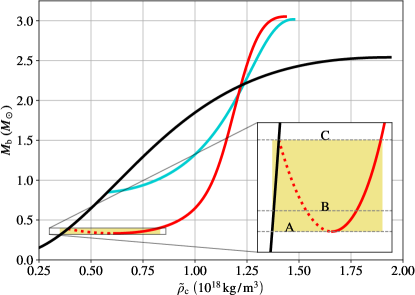
Figure 1: Baryon mass vs the central density $\tilde{\rho}_{\text{c}}=\tilde{\rho}(r{=}0)$ diagrams under general relativity (black) and STTs with spontaneous scalarization (red, turquoise). Turquoise: $\beta=-10$, $m_{\phi}=1\times 10^{-11}\,\text{eV}$. Red: $\beta=-40$, $m_{\phi}=4\times 10^{-11}\,\text{eV}$.

We used the numerical techniques detailed in Tuna et al. [25] to obtain the static, spherically symmetric NS solutions for the action (1), also see the “End Matter.” Both scalarized and unscalarized solutions are plotted in Fig. 1 as one-parameter families in terms of the central density of the star $\tilde{\rho}_{\text{c}}$. We use the HB equation of state (EOS) of Read et al. [26] in all cases, but results are qualitatively similar for other choices.

Our main objective is understanding the physical relevance of the solutions when there exists more than one configuration for a given number of baryons $N_{\text{b}}$ in the star, or equivalently the total baryon mass $M_{\text{b}}=m_{\text{b}}N_{\text{b}}$, where $m_{\text{b}}$ is the rest mass of a single baryon. In other words, if we are given a fixed number of baryons and there are more than one theoretical equilibrium configuration they can arrange themselves in, which one(s) are astrophysically relevant?

Let us start with the “standard” scalarization picture. The unscalarized solutions, which are also solutions in GR, are on the black curve, and the scalarized ones are on the turquoise one in Fig. 1. Scalarized solutions branch-off at a critical baryon mass $M_{\text{crit}}$, below which there is only one solution for a given baryon mass, an unscalarized one. This solution is known to be stable, hence, can be observed in principle. For $M_{\text{b}}>M_{\text{crit}}$ though, there are two possible solutions, one of them being scalarized . However, we have seen that the unscalarized solution is unstable to the growth of a scalar mode, hence it would not be observed. Thus, any existing star with these higher masses would be a scalarized one. We call this picture second-order scalarization. The naming will become clear in our phase transition discussion.

Our main interest is the first-order scalarization of the red curve in Fig. 1, which corresponds to different theory parameters $(\beta,m_{\phi})$. The scalarized section of the $M_{\text{b}}(\tilde{\rho}_{\text{c}})$ curve slopes downwards at the branch-off point $M_{\text{crit}}$ in this case, which changes the above discussion substantially. Defining the lowest mass on the scalarized branch as $M_{\text{bottom}}$, there is a single scalarized and stable equilibrium solution for $M_{\text{b}}<M_{\text{bottom}}$. There are two solutions for $M_{\text{b}}>M_{\text{crit}}$, where the unscalarized solution (black) is unstable due to the tachyonic growth, and the scalarized one (red) is stable. This is similar to second-order scalarization so far.

The novelty is in the highlighted region $M_{\text{bottom}}<M_{\text{b}}<M_{\text{crit}}$ in Fig. 1, where there are three equilibrium solutions for a given $M_{\text{b}}$. Firstly, the middle solution on the dotted curve, is unstable, hence physically irrelevant. A one parameter family of equilibrium NS solutions, such as our $M_{\text{b}}(\tilde{\rho}_{\text{c}})$, change from being stable to unstable at a turning point $\mathrm{d}M_{\text{b}}/\mathrm{d}\tilde{\rho}_{\text{c}}=0$, and the $\mathrm{d}M_{\text{b}}/\mathrm{d}\tilde{\rho}_{\text{c}}<0$ part is known to be the unstable one [28, 29, 30, 31, 14]. This instability is not necessarily due to the tachyonic scalar mode, but can also be a result of the modes of collective motion of the stellar matter.

The remaining two solutions, the scalarized star with $\mathrm{d}M_{\text{b}}/\mathrm{d}\tilde{\rho}_{\text{c}}>0$ (solid red) and the unscalarized star (black), are at least locally stable. The former is stable by being on the other side of a turning point, and the latter because there is no hydrodynamical instability on this part of the GR curve, and the tachyonic instability of the scalar is not present before $M_{\text{crit}}$. Thus, we have two physically relevant solutions sharing the same $M_{\text{b}}$.

When there are multiple equilibrium solutions that are robust against small perturbations, as is our case, we have the phenomenon of metastability. We typically call the solution with the globally lowest energy to be the stable one (or the global minimum), whereas the others are metastable. A metastable state would energetically prefer to transition to the global minimum, but this can only occur for large enough perturbations which may or may not exist in a star’s environment. Hence, both solutions are possible in reality, which makes novel astrophysical scenarios possible as we will discuss later.

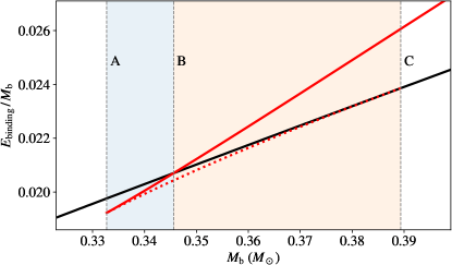
Figure 2: Fractional binding energy $(M_{\text{b}}-M_{\text{ADM}})/M_{\text{b}}$ in the highlighted region of Fig. 1.

The total energy of a NS is its ADM mass $M_{\text{ADM}}$. Hence, we can determine metastability by checking the total binding energy $E_{\rm binding}=M_{\text{b}}-M_{\text{ADM}}$ plotted in Fig. 2, which shows that metastability is not exclusive to one branch of solutions. For lower $M_{\text{b}}$ (to the left of the vertical line B) the unscalarized (black) configuration is energetically favored, and the opposite is true for higher $M_{\text{b}}$. We also see that the unstable scalarized solutions (dotted red) always have higher energy than the locally stable ones.

We closely investigated only two points on the $(\beta,m_{\phi})$ parameter space of our STT so far, but what is the prevalence of first- and second-order scalarization in general? Fig. 3 (left) shows the maximum ADM mass difference between two stars with the same baryon mass, $\Delta M$, which is a crude approximation for the energy that would be released in a transition between two states where there is no matter loss. Since it means there are metastable states, any point with a nonzero value means scalarization is first order if the STT with parameters $(\beta,m_{\phi})$ governs gravity. One can see that second-order scalarization is the dominant type even for the original scalarization model for which $m_{\phi}=0$ [8]. This clearly demonstrates our claim about the ubiquity of first-order scalarization.

Fig. 3 (right) shows the ADM mass at the branch-off point of scalarization, $M_{\text{ADM,branch}}$ only for the parameter values featuring first-order scalarization. This is relevant since it gives us a rough measure of the NS (ADM) masses where transitions from a metastable to a stable configuration can occur. Metastable solutions mostly have $M_{\text{ADM,branch}}\lesssim 0.8M_{\odot}$, which is low but astrophysically relevant [32]. We will further comment on this in our discussion.

In terms of detectability, realtively higher NS masses and higher $\Delta M$ are both desirable. This means that the prominent regions in Fig. 3 are not necessarily interesting on their own, but rather the middle region where $\Delta M$ and $M_{\text{ADM,branch}}$ are both relatively high likely provides the best observational prospects. Consider these results in the context that they are only for a specific STT. $\Delta M$ and $M_{\text{ADM,branch}}$ would vary for other, more general, STTs, providing opportunities for testing deviations from GR.

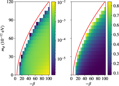
Figure 3: Dependence of scalarization characteristics on the theory parameters $(\beta,m_{\phi})$ for first order scalarization. There is no scalarization at all above the red curve [25]. Second-order scalarization occurs only in the white regions below the curve. Thus, first-order scalarization is by far the more likely outcome if scalarization occurs. Left: $\Delta M$, the maximum ADM mass difference between two stars of equal baryon mass. Right: ADM mass at the scalarization branch-off point. Both are in units of $M_{\odot}$.

Phenomenological descriptions of scalarization: The onset of scalarization has been viewed as a phase transition since the early days [10], and phenomenological explanations in terms of Landau theory have been occasionally invoked in the literature [31, 33]. Nevertheless, this has been in the context of second-order phase transitions, which only holds for second-order scalarization. Here, we show that all unusual features of first-order scalarization in the $M_{\text{bottom}}<M_{\text{b}}<M_{\text{crit}}$ region can be explained by a first-order phase transition.

In Landau theory [35, 36], one considers how the total free energy of a system changes with a quantity called the order parameter, based on the symmetries of the system. In our case, we will concentrate on the simpler $m_{\phi}=0$ case where this translates to

$$M_{\text{ADM}}=M_{0}(M_{\text{b}})+a(M_{\text{b}})Q^{2}+\frac{1}{2}b(M_{\text{b}})Q^{4}+\frac{1}{3}c(M_{\text{b}})Q^{6}.$$ (3)

The scalar charge of the star, defined as $\phi(r\to\infty)=\phi_{\infty}+Q/r+\cdots$ has been used as the order parameter $Q$ [8, 10]. In rough terms, we take a given amount of baryons $M_{\text{b}}$, and determine how the total energy of the solution changes as we dress it with scalar fields whose strength is represented by $Q$. The scalar charge is not well defined for massive scalars, but some other measure of the strength of scalarization such as the scalar field value at the center can be used in a similar vein. Only even terms are present in Eq. (3) due to the $\phi\to-\phi$ symmetry. $c(M_{\text{b}})>0$ for overall stability of the system.

Second-order scalarization occurs when $b(M_{\text{b}})>0$. We overlook $c(M_{\text{b}})$ which plays no direct role in this case. The two variables $M_{\text{b}}$ and $Q$ are actually not independent for the equilibrium solutions, i.e., the static NS solutions we studied above. For a given $M_{\text{b}}$, the physically realized $Q$ will be the one that minimizes the total energy $M_{\text{ADM}}$. For $a>0$, this is simply $Q=0$, the unscalarized solution. For $a<0$, however, $Q=0$ becomes a local maximum, an unstable equilibrium, and we get two minima at $Q=\pm(-a/b)^{1/2}$. Thus, as $a$ changes sign, the $Q\leftrightarrow-Q$ symmetry gets spontaneously broken, and a phase transition to nonzero values of $Q$ occurs continuously: physically relevant equilibria with arbitrarily small $Q$ are possible. Recall that both signs of $Q$ correspond to the same $M_{\text{b}}(\tilde{\rho}_{\text{c}})$ curve in Fig. 1.

This is a textbook example of a second-order phase transition, hence our nomenclature. In particular, $a(M_{\text{b}})$ changes sign at a critical baryon mass where stable scalarized solutions appear, which is the $M_{\text{crit}}$ from the previous section. This phenomenological explanation goes back to the earliest works on the topic [10, 31].

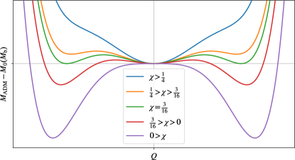
Figure 4: The Landau ansatz in Eq. (3) in the case $b<0$, plotted for different values of the parameter $\chi\equiv ac/b^{2}$. This is the case of a first-order phase transition.

First-order scalarization occurs when $b(M_{\text{b}})<0$, for which $c(M_{\text{b}})>0$ is also relevant. The behavior of $M_{\text{ADM}}(Q)$ changes drastically depending on the parameter $\chi\equiv ac/b^{2}$ as seen in Fig. 4. To start with, for $\chi>1/4$, the only equilibrium point and the global minimum of Eq. (3) is at $Q=0$. There is only a single stable, unscalarized configuration for a given $M_{\text{b}}$, corresponding to the region to the left of the line $A$ in Fig. 2.

As $M_{\text{b}}$ increases, $\chi$ drops below $1/4$ and local maxima ($-$) and outer local minima ($+$) appear at

$$Q^{2}_{\pm}=\left[-b/(2c)\right]\left(1\pm\sqrt{1-4\ ac/b^{2}}\ \right).$$ (4)

However, the global minimum is still located at $Q=0$ if $\chi>3/16$. This is the case where the unscalarized ($Q=0$) solution is the globally stable one, and the stable scalarized solutions are metastable. In Fig. 2, this corresponds to the region between vertical lines A and B. The local maxima are also equilibrium solutions, they are the unstable scalarized configurations (dotted line in Fig. 2) which have the highest total energy, i.e., the lowest binding energy among the equilibria.

As $M_{\text{b}}$ increases further, we arrive at $\chi=3/16$, where the energies at $Q=0$ and the outer minima become equal. This corresponds to line B in Fig. 2, and it is the actual point of the first-order phase transition. If $\chi$ becomes less than $3/16$, i.e., to the right of line B, the scalarized solution at $Q_{+}$ becomes the globally stable one, and the unscalarized stars become metastable. Note that, at the point of transition, the global minimum jumps discontinuously from $Q=0$ to one of $Q=\pm Q_{+}$, which is a hallmark of first-order phase transitions.

Further increasing $M_{\text{b}}$ brings us to $a=0$, for which the maxima at $Q=\pm Q_{-}$ join the local minimum at $Q=0$. This corresponds to the line C in Fig. 2. For negative values of $a$, we have a local maximum at $Q=0$, and minima at $Q=\pm Q_{+}$. This corresponds to having one unstable GR solution and one stable scalarized solution, which is the region to the right of line C.

The phase transition picture elucidates many points in our numerical results which previously had no clear reason. For example, unstable solutions are not necessarily energetically disfavored in general, but the unstable scalarized stars always have the lowest binding energy in Fig. 2. In Fig. 4, this is a trivial point since a local maximum between two local minima has to have the highest energy. The list continues for other features like (i) the stable scalarized stars being metastable at lower $M_{\text{b}}$ and becoming the global minimum only with increasing $M_{\text{b}}$, (ii) the branch continuously connected to the GR solutions being unstable and (iii) the unstable scalarized stars always having lower scalar charge compared to the scalarized ones: $Q_{-}<Q_{+}$ (not plotted here).

Discussion: We have demonstrated that first-order scalarization is the norm for our choice of STT action (1), but we also expect this to be a common occurrence. Scalarization is now known to be a generic phenomenon for various possible couplings between a scalar field and the metric [12, 13, 38, 9]. There are negative cases, as our preliminary analysis indicates that the coupling choice $A(\phi)=\cosh\left(\sqrt{3}\beta\phi\right)^{1/3\beta}$ [14, 39] features first-order scalarization less prominently. On the other hand, some other STTs feature first-order transitions even more prominently than Eq. (1). For example, scalarization of both black holes and NSs in scalar-Gauss-Bonnet theories are known to preferentially have first-order scalarization when couplings are explicitly enhanced in higher orders, e.g. $A(\phi)=e^{\beta\phi^{2}/2+\gamma\phi^{4}/4}$ [19, 21, 20, 22, 23].

Our phase transition picture already has a simple and powerful explanation for the above results. Changing the $\phi^{4}$ term in the expansion of $A(\phi)$ directly modifies the higher order expansion coefficients in our Landau ansatz (3), specifically $b$. Recalling that the main difference between a first and second-order transition is the sign of $b$, we can see how these higher order terms can determine the order of the phase transition. However, we emphasize that explicitly modifying the coupling or some form of fine tuning is not necessary for first-order scalarization by any means, as is clear from our choice of $A(\phi)$ here. Overall, we aim to study first-order scalarization for the most general STTs in order to devise more comprehensive tests for these theories.

In terms of observational prospects, the specific examples we gave are most relevant for lower mass NSs since we concentrated on the onset of scalarization. There are recently proposed theoretical scenarios for these such as formation of NSs down to masses of $0.1M_{\odot}$ in accretion disks [40], and tidal disruption events in black hole–NS mergers where part of the NS mass can be ripped out [41, 42]. How a first-order transition would behave during the birth of a NS in a supernova explosion is also not known in detail [11], which might be relevant. There is already some work about first-order phase transition near the maximum allowed NS masses, for which possible astrophysical signals have been studied [18]. We expect these studies to be readily adaptable to the transitions at lower stellar masses we studied above. Lastly, we reiterate that what we considered in action (1) is the original and most popular scalarization theory, but it is one scalar coupling choice for a specific $A(\phi)$. We expect other models of scalarization to have different characteristics, where different NS mass ranges are possible or even dominant for first-order scalarization. Studying these more general theories and how to test them via discontinuous phase transitions are major future research directions.

The phase transition order depends on the sign of $b$. Let us remark that the parameters $a,b,c$, as well as the function $M_{0}$ and the critical mass $M_{\text{crit}}$ depend on the parameters of the theory, $(\beta,m_{\phi})$, and also the EOS. For simplicity let us focus on the $\beta$ dependence, i.e. $b=b(M_{\text{b}},\beta)$. The fact that the order of the phase transition changes at some point as $\beta$ becomes more and more negative means that $b$ changes sign as $\beta$ drops below a critical value $\beta_{\text{crit}}<0$. When $\beta=\beta_{\text{crit}}$, we have a point where $a$ and $b$ vanish simultaneously, i.e., the point $(\beta=\beta_{\text{crit}},M_{\text{b}}=M_{\text{crit}}(\beta_{\text{crit}}))$. Such a point is called a tricritical point [35, 36], and it separates a line of second-order phase transitions on the $(\beta,M_{\text{b}})$ plane from a line of first-order ones. Spontaneous scalarization at $\beta_{\text{crit}}$ features special characteristics whose study is another possible future research topic. Similarly, other aspects of the voluminous phase transition literature can be a source of other surprising results for gravitational phase transitions.

This study was supported by the Scientific and Technological Research Council of Turkey (TÜBİTAK) Grant Number 122F097. Authors thank TÜBİTAK for its support, and Daniela Doneva and Stoytcho Yazadjiev for helpful discussions.

End Matter

A static, spherically-symmetric metric can be put in the form

$$g_{\mu\nu}\mathrm{d}x^{\mu}\mathrm{d}x^{\nu}=-e^{\nu(r)}\mathrm{d}t^{2}+\frac{\mathrm{d}r^{2}}{1-2\mu(r)/r}+r^{2}\mathrm{d}\Omega^{2},$$ (1)

NS structures in this case can be obtained by solving the modified Tolman–Oppenheimer–Volkoff (TOV) equations. Details can be found in Tuna et al. [25].

One needs to know the nuclear matter equation of state (EOS) to solve the TOV equations. A simple choice is a polytrope that relates the pressure of nuclear matter to the rest mass density of baryons $\tilde{\rho}_{\text{r}}$ (in the Jordan frame, i.e., in the frame of the metric $\tilde{g}_{\mu\nu}$)

$$\tilde{\rho} =\tilde{\rho}_{\text{r}}+\frac{C}{\Gamma-1}\tilde{\rho}_{\text{r}}^{\Gamma},$$ (2a)

$$\tilde{p} =C\tilde{\rho}_{\text{r}}^{\Gamma},$$ (2b)

where $C$ and $\Gamma$ are constants. Note that the two equations are related by the first law of thermodynamics. This relationship is sometimes expressed in terms of the number density of baryons $\tilde{n}$, which is linearly related to the baryon rest mass density as $\tilde{\rho}_{\text{r}}=m_{\rm b}\tilde{n}$. In this study, we employ the slightly more complicated piecewise polytropic EOS introduced in Read et al. [26].

Once the TOV equations are solved, the total energy of the spacetime, the Arnowitt-Deser-Misner (ADM) mass $M_{\text{ADM}}$, is given by

$$M_{\text{ADM}}=\mu(r\to\infty).$$ (3)

Baryon mass, which is the integral of $\tilde{\rho}_{\text{r}}$ over the proper volume of the star ($r<R$) in the Jordan frame is

$$M_{\text{b}}=m_{\text{b}}N_{\text{b}}=\int_{0}^{R}\ 4\pi r^{2}\tilde{\rho}_{\text{r}}A^{3}\left(1-\frac{2\mu}{r}\right)^{-1/2}\mathrm{d}r.$$ (4)

This is the total energy we would have if we separated all the $N_{\text{b}}$ baryons in the star into distant places in a thought experiment.

References

- Abbott et al. [2016] B. P. Abbott et al. (LIGO Scientific, Virgo), Tests of general relativity with GW150914, Phys. Rev. Lett. 116, 221101 (2016), [Erratum: Phys.Rev.Lett. 121, 129902 (2018)], arXiv:1602.03841 [gr-qc] .
- Abbott et al. [2019] B. P. Abbott et al. (LIGO Scientific, Virgo), Tests of General Relativity with GW170817, Phys. Rev. Lett. 123, 011102 (2019), arXiv:1811.00364 [gr-qc] .
- Abbott et al. [2023a] R. Abbott et al. (KAGRA, VIRGO, LIGO Scientific), Population of Merging Compact Binaries Inferred Using Gravitational Waves through GWTC-3, Phys. Rev. X 13, 011048 (2023a), arXiv:2111.03634 [astro-ph.HE] .
- Abbott et al. [2023b] R. Abbott et al. (KAGRA, VIRGO, LIGO Scientific), GWTC-3: Compact Binary Coalescences Observed by LIGO and Virgo during the Second Part of the Third Observing Run, Phys. Rev. X 13, 041039 (2023b), arXiv:2111.03606 [gr-qc] .
- Arun et al. [2022] K. G. Arun et al. (LISA), New horizons for fundamental physics with LISA, Living Rev. Rel. 25, 4 (2022), arXiv:2205.01597 [gr-qc] .
- Barack et al. [2019] L. Barack et al., Black holes, gravitational waves and fundamental physics: a roadmap, Class. Quant. Grav. 36, 143001 (2019), arXiv:1806.05195 [gr-qc] .
- Gendreau and Arzoumanian [2017] K. Gendreau and Z. Arzoumanian, Searching for a pulse, Nat. Astron. 1, 895 (2017).
- Damour and Esposito-Farèse [1993] T. Damour and G. Esposito-Farèse, Nonperturbative strong-field effects in tensor-scalar theories of gravitation, Phys. Rev. Lett. 70, 2220 (1993).
- Doneva et al. [2024] D. D. Doneva, F. M. Ramazanoğlu, H. O. Silva, T. P. Sotiriou, and S. S. Yazadjiev, Spontaneous scalarization, Rev. Mod. Phys. 96, 015004 (2024), arXiv:2211.01766 [gr-qc] .
- Damour and Esposito-Farese [1996] T. Damour and G. Esposito-Farese, Tensor-scalar gravity and binary-pulsar experiments, Phys. Rev. D 54, 1474 (1996), arXiv:gr-qc/9602056 .
- Sperhake et al. [2017] U. Sperhake, C. J. Moore, R. Rosca, M. Agathos, D. Gerosa, and C. D. Ott, Long-lived inverse chirp signals from core collapse in massive scalar-tensor gravity, Phys. Rev. Lett. 119, 201103 (2017), arXiv:1708.03651 [gr-qc] .
- Doneva and Yazadjiev [2018] D. D. Doneva and S. S. Yazadjiev, New Gauss-Bonnet Black Holes with Curvature-Induced Scalarization in Extended Scalar-Tensor Theories, Phys. Rev. Lett. 120, 131103 (2018), arXiv:1711.01187 [gr-qc] .
- Silva et al. [2018] H. O. Silva, J. Sakstein, L. Gualtieri, T. P. Sotiriou, and E. Berti, Spontaneous scalarization of black holes and compact stars from a Gauss-Bonnet coupling, Phys. Rev. Lett. 120, 131104 (2018), arXiv:1711.02080 [gr-qc] .
- Mendes and Ortiz [2018] R. F. P. Mendes and N. Ortiz, New class of quasinormal modes of neutron stars in scalar-tensor gravity, Phys. Rev. Lett. 120, 201104 (2018), arXiv:1802.07847 [gr-qc] .
- Herdeiro et al. [2018] C. A. R. Herdeiro, E. Radu, N. Sanchis-Gual, and J. A. Font, Spontaneous Scalarization of Charged Black Holes, Phys. Rev. Lett. 121, 101102 (2018), arXiv:1806.05190 [gr-qc] .
- Herdeiro et al. [2021] C. A. R. Herdeiro, E. Radu, H. O. Silva, T. P. Sotiriou, and N. Yunes, Spin-induced scalarized black holes, Phys. Rev. Lett. 126, 011103 (2021), arXiv:2009.03904 [gr-qc] .
- Berti et al. [2021] E. Berti, L. G. Collodel, B. Kleihaus, and J. Kunz, Spin-induced black-hole scalarization in Einstein-scalar-Gauss-Bonnet theory, Phys. Rev. Lett. 126, 011104 (2021), arXiv:2009.03905 [gr-qc] .
- Kuan et al. [2022] H.-J. Kuan, A. G. Suvorov, D. D. Doneva, and S. S. Yazadjiev, Gravitational Waves from Accretion-Induced Descalarization in Massive Scalar-Tensor Theory, Phys. Rev. Lett. 129, 121104 (2022), arXiv:2203.03672 [gr-qc] .
- Doneva and Yazadjiev [2022] D. D. Doneva and S. S. Yazadjiev, Beyond the spontaneous scalarization: New fully nonlinear mechanism for the formation of scalarized black holes and its dynamical development, Phys. Rev. D 105, L041502 (2022), arXiv:2107.01738 [gr-qc] .
- Doneva et al. [2022] D. D. Doneva, L. G. Collodel, and S. S. Yazadjiev, Spontaneous nonlinear scalarization of Kerr black holes, Phys. Rev. D 106, 104027 (2022), arXiv:2208.02077 [gr-qc] .
- Doneva et al. [2023] D. D. Doneva, C. J. Krüger, K. V. Staykov, and P. Y. Yordanov, Neutron stars in Gauss-Bonnet gravity: Nonlinear scalarization and gravitational phase transitions, Phys. Rev. D 108, 044054 (2023), arXiv:2306.16988 [gr-qc] .
- Pombo and Doneva [2023] A. M. Pombo and D. D. Doneva, Effects of mass and self-interaction on nonlinear scalarization of scalar-Gauss-Bonnet black holes, Phys. Rev. D 108, 124068 (2023), arXiv:2310.08638 [gr-qc] .
- Staykov and Doneva [2024] K. V. Staykov and D. D. Doneva, Nonlinear black hole scalarization in multi-scalar Gauss-Bonnet gravity, J. Phys. Conf. Ser. 2719, 012007 (2024).
- Ramazanoğlu and Pretorius [2016] F. M. Ramazanoğlu and F. Pretorius, Spontaneous Scalarization with Massive Fields, Phys. Rev. D93, 064005 (2016), arXiv:1601.07475 [gr-qc] .
- Tuna et al. [2022] S. Tuna, K. I. Ünlütürk, and F. M. Ramazanoğlu, Constraining scalar-tensor theories using neutron star mass and radius measurements, Phys. Rev. D 105, 124070 (2022), arXiv:2204.02138 [gr-qc] .
- Read et al. [2009] J. S. Read, B. D. Lackey, B. J. Owen, and J. L. Friedman, Constraints on a phenomenologically parametrized neutron-star equation of state, Phys. Rev. D 79, 124032 (2009), arXiv:0812.2163 [astro-ph] .
- Note [1] There is a symmetry for our choice of , which means each scalarized solution in the figure represents two configurations with opposite scalar field parity. We will be talking about points on the scalarized branches of the curve as if they are single solutions to avoid confusion, since they look as such on the curves.
- Sorkin [1981] R. Sorkin, A Criterion for the onset of instability at a turning point, Astrophys. J. 249, 254 (1981).
- Sorkin [1982] R. D. Sorkin, A Stability criterion for many-parameter equilibrium families, Astrophys. J. 257, 847 (1982).
- Shapiro and Teukolsky [1983] S. L. Shapiro and S. A. Teukolsky, Black Holes, White Dwarfs, and Neutron Stars: The Physics of Compact Objects (WILEY‐VCH, 1983).
- Harada [1998] T. Harada, Neutron stars in scalar tensor theories of gravity and catastrophe theory, Phys. Rev. D 57, 4802 (1998), arXiv:gr-qc/9801049 .
- Doroshenko et al. [2022] V. Doroshenko, V. Suleimanov, G. Pühlhofer, and A. Santangelo, A strangely light neutron star within a supernova remnant, Nature Astron. 6, 1444 (2022).
- Khalil et al. [2019] M. Khalil, N. Sennett, J. Steinhoff, and A. Buonanno, Theory-agnostic framework for dynamical scalarization of compact binaries, Phys. Rev. D 100, 124013 (2019), arXiv:1906.08161 [gr-qc] .
- Note [2] The end, rather than the beginning, of scalarization was called a first-order phase transition in \rev@citetKuan:2022oxs, though this study was not specifically concerned with a phenomenological analysis.
- Plischke and Bergersen [2006] M. Plischke and B. Bergersen, Equilibrium Statistical Physics (World Scientific, 2006).
- Goldenfeld [2018] N. Goldenfeld, Lectures on Phase Transitions and the Renormalization Group (CRC Press, 2018).
- Note [3] We are only interested in solutions with , it therefore plays no role in our phase transition picture. However, in general, has an effect on scalarization analogous to the effect of an external magnetic field on magnetization.
- Andreou et al. [2019] N. Andreou, N. Franchini, G. Ventagli, and T. P. Sotiriou, Spontaneous scalarization in generalized scalar-tensor theory, Phys. Rev. D99, 124022 (2019), arXiv:1904.06365 [gr-qc] .
- Demirboğa et al. [2023] E. S. Demirboğa, Y. E. Şahin, and F. M. Ramazanoğlu, Subtleties in constraining gravity theories with mass-radius data, Phys. Rev. D 108, 024028 (2023), arXiv:2303.01910 [gr-qc] .
- Metzger et al. [2024] B. D. Metzger, L. Hui, and M. Cantiello, Fragmentation in Gravitationally Unstable Collapsar Disks and Subsolar Neutron Star Mergers, Astrophys. J. Lett. 971, L34 (2024), arXiv:2407.07955 [astro-ph.HE] .
- Stephens et al. [2011] B. C. Stephens, W. E. East, and F. Pretorius, Eccentric Black Hole-Neutron Star Mergers, Astrophys. J. Lett. 737, L5 (2011), arXiv:1105.3175 [astro-ph.HE] .
- East et al. [2012] W. E. East, F. Pretorius, and B. C. Stephens, Eccentric black hole-neutron star mergers: effects of black hole spin and equation of state, Phys. Rev. D 85, 124009 (2012), arXiv:1111.3055 [astro-ph.HE] .