Graph Canonical Correlation Analysis

Abstract

Canonical correlation analysis (CCA) is a widely used technique for estimating associations between two sets of multi-dimensional variables. Recent advancements in CCA methods have expanded their application to decipher the interactions of multiomics datasets, imaging-omics datasets, and more. However, conventional CCA methods are limited in their ability to incorporate structured patterns in the cross-correlation matrix, potentially leading to suboptimal estimations. To address this limitation, we propose the graph Canonical Correlation Analysis (gCCA) approach, which calculates canonical correlations based on the graph structure of the cross-correlation matrix between the two sets of variables. We develop computationally efficient algorithms for gCCA, and provide theoretical results for finite sample analysis of best subset selection and canonical correlation estimation by introducing concentration inequalities and stopping time rule based on martingale theories. Extensive simulations demonstrate that gCCA outperforms competing CCA methods. Additionally, we apply gCCA to a multiomics dataset of DNA methylation and RNA-seq transcriptomics, identifying both positively and negatively regulated gene expression pathways by DNA methylation pathways.

1 Introduction

Canonical Correlation Analysis (CCA) is one of the most widely used methods for exploring relationships between two sets of high-dimensional data (Hotelling, 1936; Yang et al., 2019; Zhuang et al., 2020). In biomedical data analysis, for example, CCA has been applied to study the coupling between structural and functional brain imaging variables in neuroscience research and to examine intercorrelated pathways between epigenetic and transcriptomic measures (i.e., multi-omics) in molecular biology research (Zhou et al., 2024; Lee et al., 2024). In most CCA models, the objective is to identify linear combinations of the variables in each dataset, known as canonical variables, that are maximally correlated. However, traditional CCA has limited applications in high-dimensional data analysis. As the number of variables increases, canonical correlations tend to be inflated, leading to overly high estimates—similar to the inflation of R-squared values in linear regression when overfitting occurs. Furthermore, when the sample size is smaller than the number of variables, CCA cannot be computed due to the presence of non-invertible matrices (Lê Cao et al., 2009).

To address this limitation, various CCA methods in a sparse setup have been studied. Witten and Tibshirani (2009); Witten et al. (2009) developed CCA methods with penalties (i.e. $\ell_{1}$) imposed on canonical vectors. Following this work, Tenenhaus et al. (2014) generalizes penalty functions of CCA for 3 or more data sets. Although these CCA methods with $\ell_{1}$ penalization perform well to identify the maximum correlations between the two sets of multi-dimensional variables, they may not fully recover the sets of correlated variables in the two sets (Bühlmann and Van De Geer, 2011). The partially recovered sets of correlated variables may be limited to revealing the systematic relationships between the two sets of variables. For example, in our motivating multi-omics dataset, we aim to investigate how DNA methylation variables regulate RNA expression. Existing CCA methods are limited in uncovering underlying intercorrelated pathways and estimating correlations between them.

To bridge the gap, we propose a graph Canonical Correlation Analysis (gCCA) model that simultaneously reveals the correlated variables and estimates the canonical correlation based on the graph patterns of the cross-correlation matrix of the two data sets. By leveraging the graph patterns, gCCA can identify the correlated modules/pathways in the two sets and estimate canonical correlations as a measure of association between the modules. This often provides more interpretable findings for biomedical research, for example, to extract systematically related multi-omics/imaging-omics data revealing correlated pathways. In addition, we theoretically demonstrate a minimum sample size condition that guarantees the performance of gCCA to identify all correlated variables between two datasets with high probability. Lastly, we establish a finite-sample guarantee that demonstrates a square-root convergence rate for canonical correlation estimation through the identification of associated variables.

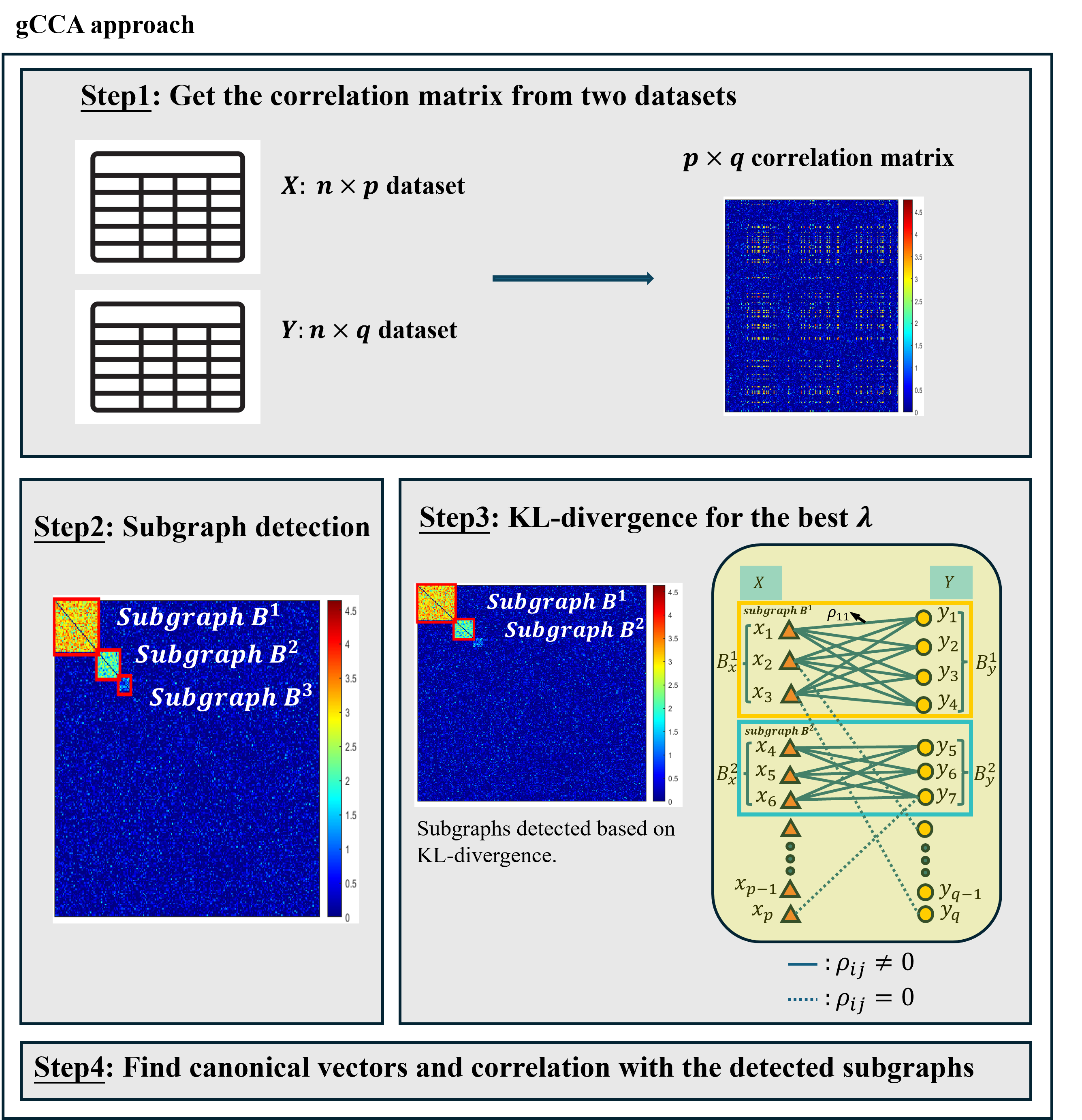
Figure 1: Pipeline to detect associated variables for associations in two different data sets by gCCA. Step 1 shows the correlation matrix calculated from two joint datasets. Step 2 illustrates the subgraphs detected by the greedy algorithm for a specific tuning parameter $\lambda$. Step 3 showcases the two optimal subgraphs based on the optimal tuning parameter and the connections of variables in and outside the subgraphs. Lastly, Step 4 is the calculation of canonical vectors and correlation.

Figure 1 provides an overview of the gCCA method. The procedure begins with calculating the sample cross-correlation matrix between two sets of variables from the same subjects. Following this, gCCA is applied with a set of tuning parameter values to identify graph patterns, which we refer to as subgraphs with strong associations throughout this paper. The optimal tuning parameter is then selected objectively. The extracted subgraphs allow us to interpret the interacted modules or pathways within the two sets of variables. Finally, we compute the canonical vectors and correlations to quantify the strength of associations between the two data sets based on the extracted graph patterns.

The organization is as follows. In Section 2, we introduce the background of CCA, graph Canonical Correlation Analysis (gCCA) model, and a greedy algorithm for gCCA to detect subgraphs in which variables have strong associations. In addition, we introduce a set of assumptions and theoretical results based on the assumption in Section 3. Next, we evaluate gCCA using synthetic datasets in Section 4 and apply it to the motivating dataset in Section 5 to study the interactions between DNA methylations and transcriptomics in patients with cancer. The paper concludes with a discussion.

2 Methods

2.1 Data structure

In this work, we analyze the associations of two datasets ${\bf X}\in\mathbb{R}^{n\times p}$ and ${\bf Y}\in\mathbb{R}^{n\times q}$, where the $s$-th rows of $\mathbf{X}$ and $\mathbf{Y}$ represent the measurements of $s$-th subject for $s=1,\dots,n$, denoted by $X^{(s)}=(X_{1}^{(s)},\dots,X_{p}^{(s)})$ and $Y^{(s)}=(Y_{1}^{(s)},\dots,Y_{q}^{(s)})$, which are samples of random vectors $(X,Y)$. Suppose without loss of generality that the datasets each have been centered and scaled to have sample mean zero and sample second moment 1 for each column component of ${\bf X}$ and ${\bf Y}$. In this work, we do not impose specific distributional assumptions on $X$ and $Y$, but instead conduct our analysis under a set of general assumptions, which will be formally introduced and discussed in the next sections.

2.2 Background

CCA is a statistical method used to explore the relationships between two datasets. CCA considers the following maximization problem:

$$\text{max}_{a,b}(a^{\top}{\bf X}^{\top}{\bf Y}b)~\text{subject~to}~a^{\top}{\bf X}^{\top}{\bf X}a\leq 1~\text{and}~b^{\top}{\bf Y}^{\top}{\bf Y}b\leq 1,$$

where the vectors $a$ and $b$ and the correlation are said to be canonical vectors and canonical correlation if they attain the above maximization.

In the classical canonical correlation analysis, the canonical vectors $a$ and $b$ include nonzero loadings for all $X$ and $Y$ variables. However, in a high-dimensional setting with $p,q\gg n$, the goal is to identify which subsets of $X$ are associated with subsets $Y$ and estimate the measure of associations, as the canonical correlation with the full dataset is overly high due to estimation bias caused by overfitting. To ensure the sparsity, shrinkage methods are commonly used. For example, Witten et al. (2009) propose sparse canonical correlation analysis (sCCA). The criterion of sCCA can be in general expressed as follows:

$$\max_{a,b}a^{\top}{\bf X}^{\top}{\bf Y}b~\text{subject to}~a^{\top}{\bf X}^{\top}{\bf X}a\leq 1,~b^{\top}{\bf Y}^{\top}{\bf Y}b\leq 1,~P_{1}(a)\leq k_{1},~P_{2}(b)\leq k_{2},$$

where $P_{1}$ and $P_{2}$ are convex penalty functions for penalization for $a$ and $b$ with positive constants $k_{1}$ and $k_{2}$, respectively. A representative penalty function is a $\ell_{1}$ penalty function such that $P_{1}(a)=\|a\|_{1}$ and $P_{2}(b)=\|b\|_{1}$. sCCA imposes zero loadings in canonical vectors and thus only selects subsets of correlated $X$ and $Y$. However, sCCA methods may neither fully recover correlated $X$ and $Y$ pairs nor capture the multivariate-to-multivariate linkage patterns (see Figure 3) because the $\ell_{1}$ shrinkage tends to select only a small subset from the associated variables of $X$ and $Y$.

2.3 Graph Canonical Correlation Analysis

To capture the systematic correlations between $X$ and $Y$ and estimate their strength, we present the gCCA method to solve the following objective function:

$$\max_{a,b}a^{\top}{\bf X}^{\top}{\bf Y}b~\text{subject~to}~a^{\top}{\bf X}^{\top}{\bf X}a\leq 1,~b^{\top}{\bf Y}^{\top}{\bf Y}b\leq 1~\text{and}~\|a\|_{0}\leq k_{1},~\|b\|_{0}\leq k_{2}.$$ (1)

where $\|\cdot\|_{0}$ is the $\ell_{0}$ norm and $k_{1}$ and $k_{2}$ are positive constants. The goal is to capture maximum correlations between $X$ and $Y$ with the minimal subsets of $X$ and $Y$ included. Therefore, gCCA can recover correlated components of $X$ and $Y$ and better estimate the canonical correlation while suppressing the false positive correlations. However, in practice, optimizing the gCCA objective function (1) is challenging due to the non-convexity and cardinality constraint, which renders it NP-hard (Natarajan, 1995; Bertsimas et al., 2016). Thus, we implement (1) using a graph-based approach.

We first define $G=(U,V,E)$ as a bipartite graph, where $U$ and $V$ are disjoint sets of nodes corresponding to the variables of $X$ and $Y$, respectively, and $E$ is the set of binary edges representing the presence of correlations between the variables of $X$ and $Y$. We utilize the concept of a bipartite graph to emphasize edges connecting $X$ and $Y$, rather than those within each disjoint node set.

The adjacency matrix ${\bf A}\in\mathbb{R}^{p\times q}$ represents the edges in the node sets $U$ and $V$. The adjacency matrix $A=[A_{ij}]$ is a matrix-based representation of the edge set $E$. Each entry $A_{ij}$ in the matrix is binary for the bipartite binary graph $G$ and has a relationship with the edge $e_{ij}$ between the node $u_{i}$ and $v_{j}$ as follows: $A_{ij}=1$, if $e_{ij}\in E$ (edge exists), $A_{ij}=0$, otherwise. Specifically, we let $A_{ij}=1$ if $\text{Corr}(X_{i},Y_{j})=\rho_{ij}\neq 0$ and $A_{ij}=0$ otherwise. We have $|U|=p,|V|=q$ and $|E|=\sum_{i\in[p],i\in[q]}A_{ij}\leq pq$. We use biclique (complete bipartite) subgraphs $B_{c}=(U_{c},V_{c},E_{c})$ for $c=1,\cdots,C$ to characterize this pattern, where

$$E_{c}=\{e_{ij}:A_{ij}=1~\text{for~all}~(i,j)\in U_{c}\otimes V_{c}\},$$

is the edge set of the biclique subgraph with the disjoint node sets $U_{c}$ and $V_{c}$ and $I\otimes J$ for two sets $I$ and $J$ represents $\{(i,j):i\in I~\text{and}~j\in J\}$. Let $I_{X}=\cup_{c=1}^{C}U_{c}$ and $I_{Y}=\cup_{c=1}^{C}V_{c}$ be the index sets corresponding to the associated variables of $X$ and $Y$, respectively, which are denoted by $X_{0}$ and $Y_{0}$. Given $B=\{B_{c}\}_{c=1}^{C}$ and ${\bf X}_{0}$ and ${\bf Y}_{0}$, which are the subsets of ${\bf X}$ and ${\bf Y}$ corresponding to $X_{0}$ and $Y_{0}$, respectively, the objective function (1) can be re-written as

$$\max_{a,b}a^{\top}{\bf X}_{0}^{\top}{\bf Y}_{0}b~~~\text{subject to}~a^{\top}{\bf X}^{\top}_{0}{\bf X}_{0}a\leq 1,~b^{\top}{\bf Y}^{\top}_{0}{\bf Y}_{0}b\leq 1,$$ (2)

with constraints $|I_{X}|\leq k_{1}$ and $|I_{Y}|\leq k_{2}$.

2.4 Estimation

In practice, neither biclique subgraphs $\{B_{c}\}_{c=1}^{C}$ nor corresponding variables $I_{X}$ and $I_{Y}$ are known. We estimate $U_{c}$ and $V_{c}$ (i.e., $I_{X}$ and $I_{Y}$) by the following objective function

$$f_{\lambda}(B,\varepsilon)=\sum_{c=1}^{C}\frac{\sum_{(i,j):e_{ij}\in E_{c}}|R_{ij}^{\varepsilon}|}{(|U_{c}||V_{c}|)^{\lambda}},$$ (3)

where $R_{ij}$ is a sample correlation of $X_{i}$ and $Y_{j}$ for a dataset with sample size $n$; $R_{ij}^{\varepsilon}=R_{ij}I(|R_{ij}|>\varepsilon)$; $\varepsilon\in(0,1)$ is a threshold value for cutting off absolute correlation values; $\lambda\in[0.5,1]$ is a tuning parameter. A greater $\lambda$ imposes a stricter penalty resulting in denser extracted subgraphs $\{B_{c}\}$ (i.e., higher density) yet covering a smaller number of edges with $|R_{ij}|>\varepsilon$. In (3), $|U_{c}|$ and $|V_{c}|$ are equivalent to the $\ell_{0}$ norm for associated variables between $X$ and $Y$ in $\{B_{c}\}_{c=1}^{C}$, where $\sum_{c=1}^{C}|U_{c}|=\|a\|_{0}$ and $\sum_{c=1}^{C}|V_{c}|=\|b\|_{0}$.

By implementing (3), we estimate a canonical correlation using estimated $\widehat{I}_{X}$ and $\widehat{I}_{Y}$ from $\{\widehat{B}_{c}\}_{c=1}^{C}$ as follows:

$$\widehat{a}=u_{1}({\bf X}[,\widehat{I}_{X}]^{\top}{\bf Y}[,\widehat{I}_{Y}])~~\text{and}~~\widehat{b}=v_{1}({\bf X}[,\widehat{I}_{X}]^{\top}{\bf Y}[,\widehat{I}_{Y}]),$$ (4)

where $u_{1}(M)$ and $v_{1}(M)$ are the left and right singular vectors corresponding to the first singular value of a matrix $M$, respectively; for a matrix $M\in\mathbb{R}^{n\times q}$ and integer set $I=(i_{1},i_{2},\dots,i_{q_{0}})\subset[q]$, $M[,I]$ represent the submatrix of $M$ with $(i_{1},i_{2},\dots,i_{q_{0}})$-th columns. The estimated canonical correlation is

$$\widehat{\rho}_{c}=\frac{\widehat{a}^{\top}{\bf X}[,\widehat{I}_{X}]^{\top}{\bf Y}[,\widehat{I}_{Y}]\widehat{b}}{\sqrt{(\widehat{a}^{\top}{\bf X}[,\widehat{I}_{X}]^{\top}{\bf X}[,\widehat{I}_{X}]\widehat{a})(\widehat{b}^{\top}{\bf Y}[,\widehat{I}_{Y}]^{\top}{\bf Y}[,\widehat{I}_{Y}]\widehat{b}})}.$$ (5)

The details of the estimation of $I_{X}$ and $I_{Y}$ will be described as follows.

Greedy algorithm for (3): We first implement the main gCCA objective function (3) in two steps: $\{\widehat{B}_{c}\}_{c=1}^{C}$ estimation by (3) and canonical correlation estimation by (4) and (5). Since the computations of (4) and (5) are straightforward, we focus on the implementation of the optimization of $f_{\lambda}(B,\varepsilon)$ in (3) with respect to $B$ using a greedy algorithm.

Algorithm 1 outlines a pseudo-code for the greedy algorithm. This algorithm begins with two data sets ${\bf X}$ and ${\bf Y}$, which is centered and standardized, threshold $\varepsilon$, and values of tuning parameter $\bm{\lambda}=(\lambda_{1},\lambda_{2},\dots,\lambda_{g_{0}})$. Let $\circ$ be the Hadamard product (i.e., element-wise product) between matrices of the same dimensions, and for a matrix ${\bf M}$, we define

$$(I({\bf M}>\varepsilon))_{ij}=\left\{\begin{array}[]{@{}lr@{}}1,&\text{if}~M_{ij}>\varepsilon,\\ 0,&\text{otherwise}.\end{array}\right.$$

We define the truncated absolute sample correlation matrix, denoted by $|\mathbf{R}^{\varepsilon}|\in\mathbb{R}^{p\times q}$, as follows:

$$|\mathbf{R}^{\varepsilon}|=|\mathbf{R}|\circ I(|\mathbf{R}|>\varepsilon),$$

where $\mathbf{R}=\mathbf{X}^{\top}\mathbf{Y}$ is the sample correlation matrix with a sample of size $n$. We initialize the process with $\mathbf{R}^{1,1}=|\mathbf{R}^{\varepsilon}|$, $J^{1,1}_{X}=[p]$ and $J^{1,1}_{Y}=[q]$. Let $\mathbf{R}^{c,t}$ denote the active matrix and $J^{c,t}_{X}$ and $J^{c,t}_{Y}$ do the active sets of rows $(X)$ and columns $(Y)$ of the matrix $|\mathbf{R}^{\varepsilon}|$, respectively, at time $t$ for the $c$-th subgraph. The matrix $\mathbf{R}^{c,t}$ is defined as $\mathbf{R}^{c,t}=|\mathbf{R}^{\varepsilon}|[J^{c,t}_{X},J^{c,t}_{Y}]$.

Define $u^{c,t}=\text{vec}(J_{X}^{c,t})$ and $v^{c,t}=\text{vec}(J_{Y}^{c,t})$, where $\text{vec}(I)$ represent the vectorization of $I$ in the increasing order for a set $I$. For a given $\lambda_{g}$, at time $t$ for the $c$-th subgraph extraction, we calculate the row and column means of the active matrix, denoted by $\text{r.means}(\mathbf{R}^{c,t})$ and $\text{c.means}(\mathbf{R}^{c,t})$, such that

$$\text{r.means}(\mathbf{R}^{c,t})=\left(\frac{1}{|J_{Y}^{c,t}|}\sum_{j\in J_{Y}^{c,t}}|R_{u^{c,t}_{1}j}^{\varepsilon}|,\frac{1}{|J_{Y}^{c,t}|}\sum_{j\in J_{Y}^{c,t}}|R_{u^{c,t}_{2}j}^{\varepsilon}|,\dots,\frac{1}{|J_{Y}^{c,t}|}\sum_{j\in J_{Y}^{c,t}}|R_{u^{c,t}_{|J_{X}^{c,t}|}j}^{\varepsilon}|\right)$$

and

$$\text{c.means}(\mathbf{R}^{c,t})=\left(\frac{1}{|J_{X}^{c,t}|}\sum_{i\in J_{X}^{c,t}}|R_{iv^{c,t}_{1}}^{\varepsilon}|,\frac{1}{|J_{X}^{c,t}|}\sum_{i\in J_{X}^{c,t}}|R_{iv^{c,t}_{2}}^{\varepsilon}|,\dots,\frac{1}{|J_{X}^{c,t}|}\sum_{i\in J_{X}^{c,t}}|R_{iv^{c,t}_{|J_{Y}^{c,t}|}}^{\varepsilon}|\right),$$

where $R_{ij}^{\varepsilon}$’s are as in (3) and $|S|$ for a set $S$ represents the number of elements of $S$. A small row or column mean suggests that the corresponding sample correlation coefficients are closer to zero compared to others. We let the indices of the row and column with the minimum sums based on the active matrix $\mathbf{R}^{c,t}$ denoted by $\tau_{t}$ and $\phi_{t}$, respectively. We exclude row $u^{c,t}_{\tau_{t}}$ or column $v^{c,t}_{\phi_{t}}$ (the indices based on the initial active matrix $|\mathbf{R}^{\varepsilon}|$) from our active sets and update our active set as follows: if $\text{r.means}(\mathbf{R}^{c,t})_{\tau_{t}}>\text{c.means}(\mathbf{R}^{c,t})_{\phi_{t}}$,

$$J_{X}^{c,t+1}\leftarrow J_{X}^{c,t},~J_{Y}^{c,t+1}\leftarrow J_{Y}^{c,t}\backslash\{v_{\phi_{t}}^{c,t}\},~\mathbf{R}^{c,t+1}\leftarrow|\mathbf{R}^{\varepsilon}|[J_{X}^{c,t+1},J_{Y}^{c,t+1}]$$

and otherwise

$$J_{X}^{c,t+1}\leftarrow J_{X}^{c,t}\backslash\{u_{\tau_{t}}^{c,t}\},~J_{Y}^{c,t+1}\leftarrow J_{Y}^{c,t},~\mathbf{R}^{c,t+1}\leftarrow|\mathbf{R}^{\varepsilon}|[J_{X}^{c,t+1},J_{Y}^{c,t+1}].$$

We repeat this exclusion process until only one row or column remain in our active sets. At the end of the exclusion process, we designate the biclique $J^{c,t}=(J_{X}^{c,t},J_{Y}^{c,t},E^{c,t})$ maximizing the contribution of the $c$-th subgraph to the summation in (3) as the $c$-th subgraph $B_{c}=(U_{c},V_{c},E_{c})$. Figure 2 illustrates the row and column exclusion process by the greedy algorithm under the presence of a biclique subgraph.

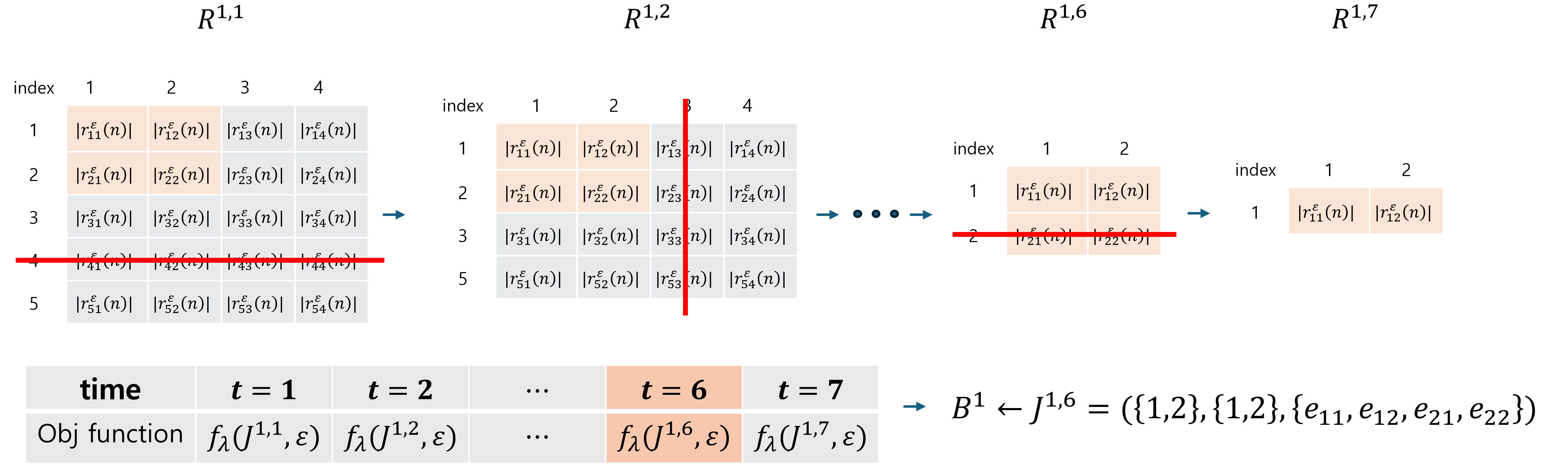
Figure 2: Row and column exclusion process by the greedy algorithm under the presence of a subgraph (size: 2 by 2) in a graph with 5 rows and 4 columns. Red and gray cells represent (unknown) associated and irrelevant variables, respectively. Solid red lines indicate the exclusion of the row or column with the lowest row or column mean among all active rows and columns. The table shows that the objective function is maximized at $t=6$ and thereby $J^{1,6}=(\{1,2\},\{1,2\},\{e_{11},e_{12},e_{21},e_{22}\})$ with $A_{ij}=1$ for all $(i,j)$ is considered the extracted biclique subgraph.

For the ($c+1$)-th subgraph extraction, we repeat the exclusion process described above with new active sets $J_{X}^{c+1,1}=J_{X}^{c,1}\backslash U_{c}$, $J_{Y}^{c+1,1}=J_{Y}^{c,1}\backslash V_{c}$ and active matrix $\mathbf{R}^{c+1,1}=\mathbf{R}[J_{X}^{c+1,1},J_{Y}^{c+1,1}]$. This process is repeated $C$ times. After that, we record the extracted subgraphs $B^{\lambda_{g}}=\{B_{c}\}_{c=1}^{C}$, which correspond to $\lambda_{g}$. We repeat this entire process for a set of tuning parameters $\{\lambda_{1},\dots,\lambda_{g_{0}}\}$. Next, we choose the optimal tuning parameter value $\lambda_{g^{\star}}$ based on the Kullback-Leibler (KL) divergence, as described below.

The tuning parameter $\lambda$ has a significant effect on the extraction of subsets. A larger value of $\lambda$ typically results in denser and smaller subsets compared to those obtained with a smaller $\lambda$. To select the optimal $\lambda$, we use the KL divergence, which measures the distance between two distributions. To describe the procedure, consider two distributions $P_{\lambda}$ and $Q$ of $D_{ij}=I(|R_{ij}|>\varepsilon)$. $P_{\lambda}$ is a distribution with subgraphs extracted based on the tuning parameter $\lambda$. $P_{\lambda}$ divides the correlation matrix into two distinct blocks: (i) the subgraphs $B^{\lambda}$ extracted by the tuning parameter $\lambda$, and (ii) the area outside the subgraphs. In block (i), $D_{ij}$ is more likely to be 1, whereas it is more likely to be 0 in block (ii). Specifically, $\{D_{ij}\}_{i,j}$ are assumed to have the following distribution:

$$D_{ij}\sim\text{Bernoulli}(\pi_{1}) \text{if}~(i,j)\in B_{c}~\text{for~some}~c\in[C]$$

$$D_{ij}\sim\text{Bernoulli}(\pi_{0}) \text{otherwise}.$$

In contrast, we consider a reference Bernoulli distribution $Q$ with no graph patterns between $X$ and $Y$ as follows:

$$D_{ij}\sim\text{Bernoulli}(\pi)~\text{for all}~(i,j).$$

The KL divergence between these two distributions can be written as

$$D_{\mathrm{KL}}\left(P_{\lambda}\|Q\right) = \sum_{(i,j)\in\cup_{c=1}^{C}(U_{c}\bigotimes V_{c})}\left(D_{ij}\pi_{1}\log\frac{\pi_{1}}{\pi}+\left(1-D_{ij}\right)\left(1-\pi_{1}\right)\log\frac{\left(1-\pi_{1}\right)}{(1-\pi)}\right)$$

$$+ \sum_{(i,j)\notin\cup_{c=1}^{C}(U_{c}\bigotimes V_{c})}\left(D_{ij}\pi_{0}\log\frac{\pi_{0}}{\pi}+\left(1-D_{ij}\right)\left(1-\pi_{0}\right)\log\frac{\left(1-\pi_{0}\right)}{(1-\pi)}\right),$$

where $\pi_{0}$ and $\pi_{1}$ are the sample mean of $D_{ij}$ outside and in the subgraphs, respectively; $\pi$ is the overall sample mean of $D_{ij}$. Then, the optimal tuning parameter is chosen so as to maximize the KL divergence as follows:

$$\lambda^{\star}=\text{argmax}_{\lambda}D_{\mathrm{KL}}\left(P_{\lambda}\|Q\right).$$

Here, we use the distribution $P_{\lambda}$ as an approximate distribution of $I(|R_{ij}|>\varepsilon)$ in subgraphs disregarding the dependencies between different $R_{ij}$. This approach, known as the variational method, is frequently employed for inference involving dependent Bernoulli variables, as the dependencies among Bernoulli random variables can lead to intractability (Murphy, 2023).

Lastly, we calculate the canonical vectors $(\widehat{a},\widehat{b})$ and correlation $\widehat{\rho}_{c}$ with the index sets of estimated associated variables $(\widehat{I}_{X},\widehat{I}_{Y})$ based on (4) and (5). The computational complexity of the greedy algorithm is $O(p+q)$ when a single subgraph is present, while it increases with the number of subgraphs, reaching a worst-case complexity of $O((p+q)^{2})$.

Algorithm 1 : Greedy Algorithm for Graph Canonical Correlation Analysis

1:Input: joint data set ${\bf X}$ and ${\bf Y}$, threshold $\varepsilon\in(0,1)$, $\bm{\lambda}=\{\lambda_{1},\dots,\lambda_{g_{0}}\}$

2:Output: canonical vectors $(\widehat{a}$, $\widehat{b})$ and canonical correlation $\widehat{\rho}_{c}$

3:Set the initial values $\mathbf{R}^{1,1}=|\mathbf{R}^{\varepsilon}|$, active set $J^{1,1}=(J_{X}^{1,1},J_{Y}^{1,1},E^{1,1}=\{e_{ij}:(i,j)\in J_{X}^{1,1}\otimes J_{Y}^{1,1}\})$ s.t $J_{X}^{1,1}=[p]$, $J_{Y}^{1,1}=[q]$

4:for $g=1,2,\dots,g_{0}$ do

5:  for $c=1,2,\dots,C$ do

6:   for $t=1,2,\dots,\text{r.size}(\mathbf{R}^{c,1})+\text{c.size}(\mathbf{R}^{c,1})-1$ do

7:     Set $\tau_{t}=\text{argmin}_{\tau}(\text{r.means}(\mathbf{R}^{c,t})_{\tau})$ and $\phi_{t}=\text{argmin}_{\phi}(\text{c.means}(\mathbf{R}^{c,t})_{\phi})$

8:     if $\text{r.means}(\mathbf{R}^{c,t})_{\tau_{t}}>\text{c.means}(\mathbf{R}^{c,t})_{\phi_{t}}$  then

9:      $J_{X}^{c,t+1}\leftarrow J_{X}^{c,t}$, and $J_{Y}^{c,t+1}\leftarrow J_{Y}^{c,t}\backslash\{v_{\phi_{t}}^{c,t}\}$, $\mathbf{R}^{c,t+1}\leftarrow\mathbf{R}^{1,1}[J_{X}^{c,t+1},J_{Y}^{c,t+1}]$

10:     else

11:      $J_{X}^{c,t+1}\leftarrow J_{X}^{c,t}\backslash\{u_{\tau_{t}}^{c,t}\}$, and $J_{Y}^{c,t+1}\leftarrow J_{Y}^{c,t}$, $\mathbf{R}^{c,t+1}\leftarrow\mathbf{R}^{1,1}[J_{X}^{c,t+1},J_{Y}^{c,t+1}]$

12:     end if

13:     $J^{c,t+1}\leftarrow(J_{X}^{c,t+1},J_{Y}^{c,t+1},E^{c,t+1}=\{e_{ij}:(i,j)\in J_{X}^{c,t+1}\otimes J_{Y}^{c,t+1}\})$

14:   end for

15:   Set $B_{c}=\text{argmax}_{J^{c,t}}f_{\lambda_{g}}(J^{c,t},\varepsilon)$, where $B_{c}=(U_{c},V_{c},E_{c})$

16:   $J^{c+1,1}_{X}\leftarrow[p]\backslash\cup^{c}_{c^{\prime}=1}U_{c^{\prime}}$, $J^{c+1,1}_{Y}\leftarrow[q]\backslash\cup^{c}_{c^{\prime}=1}V_{c^{\prime}}$, $\mathbf{R}^{c+1,1}\leftarrow\mathbf{R}^{1,1}[J^{c+1,1}_{X},J^{c+1,1}_{Y}]$

17:  end for

18:  $B^{\lambda_{g}}\leftarrow\{B_{c}\}_{c=1}^{C}$

19:end for

20:Find $g^{\star}=\text{argmax}_{g=1,2,\dots,g_{0}}D_{KL}(P_{g}||Q)$ and set $\widehat{B}\leftarrow B^{\lambda_{g^{\star}}}$, where $\widehat{B}=\{(\widehat{U}_{c},\widehat{V}_{c},\widehat{E}_{c})\}_{c=1}^{C}$

21:Set $\widehat{I}_{X}=\cup_{c=1}^{C}\widehat{U}_{c}$ and $\widehat{I}_{Y}=\cup_{c=1}^{C}\widehat{V}_{c}$

22:Return the estimated canonical vectors $(\widehat{a},\widehat{b})$ and correlation $\widehat{\rho}_{c}$ calculated based on (4) and (5)

3 Theoretical Properties of gCCA

In this section, we outline the assumptions and present the theoretical results to show the minimum sample size condition for a high probability performance guarantee of the estimation procedure of gCCA.

3.1 Assumptions

We first introduce the assumptions underlying the theories in the gCCA estimation procedure. Our first assumption concerns the distributional properties of correlation coefficients in the large cross-correlation matrix ${\bf R}$. Specifically, we assume that the sample correlation coefficients, given a sample size of $n$, satisfy a concentration property, ensuring that they are sufficiently bounded with high probability (Boucheron et al., 2003). This assumption is formulated based on the concentration inequality for the sample correlation coefficient of two bivariate normal variables, as provided in Subsection 7.1 of Supplementary Materials.

[$n^{-1/2}$ concentration of sample correlation coefficients] Let $R_{ij}$ be the sample correlation coefficient of $X_{i}$ and $Y_{j}$ with size $n>3$, which is generated from a bivariate distribution with a ground truth correlation coefficient $\rho_{ij}\in[-1+\delta,1-\delta]$ for a $0<\delta<1$. Then, for all $a>0$ and all $\rho_{ij}\in[-1+\delta,1-\delta]$, there are $s_{1},~s_{2}>0$ such that

$$P(|R_{ij}-\rho_{ij}|>a)\leq s_{1}\exp\left(-\frac{na^{2}}{2s_{2}^{2}}\right).$$

Assumption 3.1 is equivalent to the fact that there exist $s_{3},s_{4}>0$ such that $E[e^{a(R_{ij}-\rho_{ij})}]\leq s_{3}e^{s_{4}^{2}a^{2}/n}.$ for all $a>0$. This equivalence is similarly constructed to the equivalent definitions of subGaussian random variables (Vershynin, 2018). This is shown in Subsection 7.2 of Supplementary Materials. In the case with $s_{1}=2$ and $s_{3}=2$, we can say that $R_{ij}$ is $s_{2}/\sqrt{n}$-subGaussian. Second, we assume the independency of two correlation coefficients, if the indices of the two correlation coefficients are not in the subgraph.

For $(i_{1},j_{1}),~(i_{2},j_{1})\notin I_{X}\otimes I_{Y}$, $R_{i_{1}j_{1}}$ and $R_{i_{2}j_{1}}$ are independent. Similarly, for $(i_{1},j_{1}),~(i_{1},j_{2})\notin I_{X}\otimes I_{Y}$, $R_{i_{1}j_{1}}$ and $R_{i_{1}j_{2}}$ are independent. Assumption 3.1 provides a $n^{-1/2}$ concentration inequality for each correlation coefficient, while Assumption 3.1 provides a useful property of the joint distribution of two. The statement in Assumption 3.1 indeed holds for normal distributions, because a centered and standardized $d$-dimensional normal random vector has a uniform distribution in $\mathbb{S}^{d-1}$ and accordingly the angle (correlation coefficient) between two independent vectors does not provide any information about their individual directions (For further details, see 7.3 in Supplementary Materials).

3.2 Theoretical results

In this subsection, we present the main theoretical results for the gCCA estimation procedure. The first result demonstrates that the greedy algorithm can achieve full recovery of the variables with nonzero entries in the canonical vectors. The second result establishes the square-root estimation accuracy of the canonical correlation estimates obtained via gCCA.

Without loss of generality, we consider that the correlation matrix has a network structure with a single biclique subgraph $B=(U_{1},V_{1},E_{1})$, where the absolute values of correlations $|\rho_{ij}|$ for all $(i,j)\in U_{1}\otimes V_{1}$ have the values in $[\rho,w\rho]$ for some $0<\rho<1$ and $w\geq 1$. In addition, the correlation coefficients outside the subgraph are zero. For ease of presentation, we set $I_{X}=\{1,2,\dots,p_{0}\}$ and $I_{Y}=\{1,2,\dots,q_{0}\}$. Also, we consider a threshold $\varepsilon=\rho/2$. The following lemma provides bounds to ensure that the sample correlation coefficients, both within and outside the subgraph, lie within specific intervals based on the subGaussianity of sample correlation coefficients. The complete proofs of the following lemmas are provided in Supplementary Materials.

Lemma 3.1

Let $R_{ij}$ and $\rho_{ij}$ be the sample correlation coefficient with sample size $n$ and ground truth correlation of $X_{i}$ and $Y_{j}$, respectively. Then, for all $i\in[p]$ and $j\in[q]$, with probability at least $1-\delta$, we have

$$|R_{ij}-\rho_{ij}|<\sqrt{\frac{2s_{2}^{2}}{n}\log\left(\frac{s_{1}pq}{\delta}\right)}.$$

The next lemma is an anti-concentration inequality for the difference of sums of absolute sample correlation coefficients between one in a subgraph and another outside it. This inequality makes the two sums (one in a subgraph, another outside it) distinct so that we can exclude rows or columns not in subgraphs.

Lemma 3.2

For the subgraph $B$, if $n\geq(\eta/\rho)^{2}(2s_{2}\log\left(s_{1}pq/\delta\right))$, we have $\sum_{j\in I_{Y}}(|R_{i_{1}j}^{\varepsilon}|-|R_{i_{2}j}^{\varepsilon}|)>q_{0}\rho(\eta-2)/\eta$ for $i_{1}\in I_{X}$, $i_{2}\in I_{X}^{c}$, and $\eta>3$ with probability at least $1-\delta$. Similarly, $\sum_{i\in I_{X}}(|R_{ij_{1}}^{\varepsilon}|-|R_{ij_{2}}^{\varepsilon}|)>p_{0}\rho(\eta-2)/\eta$ for $j_{1}\in I_{Y}$ and $j_{2}\in I_{Y}^{c}$ with probability at least $1-\delta$.

The following lemma presents a concentration inequality for the differences of the column means of $|R_{ij}^{\varepsilon}|$ between two columns. This inequality ensures that the error terms for the sample correlation coefficients of the uncorrelated variables remain bounded over the consecutive exclusion process. As a result, the greedy algorithm can sequentially eliminate uncorrelated variables with high probability.

Lemma 3.3

Let $h_{1}$ and $h_{2}$ be bijective functions from $\{1,2,\dots,q-q_{0}\}$ to $I_{Y}^{c}$ and from $\{1,2,\dots,p-p_{0}\}$ to $I_{X}^{c}$, respectively. with probability at least $1-\delta$, if $n>\frac{\eta^{2}s_{4}^{2}}{\min(p_{0},q_{0})^{2}(\eta-2)^{2}\rho^{2}}\left(\max(p,q)(1+\log s_{3})+\log\frac{2\max(p,q)^{2}}{\delta}\right)^{2}$, we have

$$\sum_{j=1}^{t}(|R_{i_{1}h_{1}(j)}^{\varepsilon}|-|R_{i_{2}h_{1}(j)}^{\varepsilon}|)\leq\frac{\min(p_{0},q_{0})(\eta-2)\rho}{\eta},$$

for all $i_{1}\notin I_{X}$, $i_{2}\in[p]$, all $1\leq t\leq q-q_{0}$. Similarly, with probability $1-\delta$, we have

$$\sum_{i=1}^{t}(|R_{h_{2}(i)j_{1}}^{\varepsilon}|-|R_{h_{2}(i)j_{2}}^{\varepsilon}|)\leq\frac{\min(p_{0},q_{0})(\eta-2)\rho}{\eta},$$

for all $j_{1}\notin I_{Y}$, $j_{2}\in[q]$ and all $1\leq t\leq p-p_{0}$.

Now, we are ready to prove the main result based on the three lemmas above. The following result demonstrates that gCCA can detect all the related and irrelevant variables for associations of two high-dimensional variables with a high probability when the minimum sample condition is satisfied.

Theorem 3.4

For $\delta\in(0,1)$, with probability at least $1-\delta$, if

$$n>(1/\rho^{2})\left(2\sqrt{2s_{2}^{2}\log\left(2s_{1}pq/\delta\right)}+\frac{s_{4}}{2\min(p_{0},q_{0})}\left(\max(p,q)(1+\log s_{3})+\log\frac{4\max(p,q)^{2}}{\delta}\right)\right)^{2},$$

there is a set of $\lambda$ in $(0,1)$ to guarantee that the greedy algorithm for gCCA has

$$\mathbb{P}(I_{X}=\widehat{I}_{X}~\text{and}~I_{Y}=\widehat{I}_{Y})\geq 1-\delta,$$

where $\widehat{I}_{X}$ and $\widehat{I}_{Y}$ are the sets of associated variables estimated by the greedy algorithm.

proof sketch: First, based on Lemma 3.1, 3.2, and 3.3, we bound the magnitude of errors created by samples so that the associated variables are distinguishable. Then, we show that the greedy algorithm sequentially excludes uncorrelated variables from our active sets until only the associated variables remain. Next, we demonstrate that there exists a set of $\lambda$ such that our objective function is maximized at the time when only and all uncorrelated variables are excluded. Lastly, we find the value $\eta$ to minimize the sample size suggested in the lemmas.

Proof 3.5

To streamline the presentation, we define two sub-timelines $t_{X}$ and $t_{Y}$ corresponding to the rows and columns, respectively. $t_{X}-1$ and $t_{Y}-1$ are the numbers of rows and columns excluded from the initial active matrix, which is given by the truncated absolute correlation matrix $\mathbf{R}^{1}=|\mathbf{R}^{\varepsilon}|$. Here, the overall time $t$ is related to the sub-timelines by the equation $t=t_{X}+t_{Y}-1$. When a row is excluded, we update the row sub-timeline $t_{X}\leftarrow t_{X}+1$. Otherwise, we have $t_{Y}\leftarrow t_{Y}+1$.

First, we show that the greedy algorithm excludes all rows in $I_{X}^{c}$ and columns in $I_{Y}^{c}$ before excluding ones in $I_{X}$ or $I_{Y}$. Let $i_{t_{X}}$ and $j_{t_{Y}}$ denote the row and column excluded at time $t_{X}$ and $t_{Y}$ in the sub-timelines, respectively. Assume that $\{i_{t_{X}}\}_{t_{X}\in[p]}$ and $\{j_{t_{Y}}\}_{t_{Y}\in[q]}$ are the sequences of row and column exclusion. It suffices to show that the sets of the first $p-p_{0}$ excluded rows and $q-q_{0}$ columns are identical to $I_{X}^{c}$ and $I_{Y}^{c}$, which means $\{i_{t_{X}}\}_{t_{X}\in[p-p_{0}]}=I_{X}^{c}$ and $\{j_{t_{Y}}\}_{t_{Y}\in[q-q_{0}]}=I_{Y}^{c}$. Let $\{i_{t_{X}}^{\prime}\}_{t_{X}\in[p-p_{0}]}$ and $\{j_{t_{Y}}^{\prime}\}_{t_{Y}\in[q-q_{0}]}$ be reversely enumerated subsequences of $\{i_{t_{X}}\}_{t_{X}\in[p]}$ and $\{j_{t_{Y}}\}_{t_{Y}\in[q]}$, respectively, where $i_{t_{X}}^{\prime}\in I_{X}^{c}$ for all $t_{X}$ and $j_{t_{Y}}^{\prime}\in I_{Y}^{c}$ for all $t_{Y}$. Note that

$$\sum_{t_{Y}=1}^{t}(|R_{i^{\prime}j^{\prime}_{t_{Y}}}^{\varepsilon}|-|R_{ij^{\prime}_{t_{Y}}}^{\varepsilon}|)\leq\frac{\min(p_{0},q_{0})(\eta-2)\rho}{\eta}$$ (7)

for all $i\in I_{X}$, $i^{\prime}\in I_{X}^{c}$ and $t\in[q-q_{0}]$ by Lemma 3.3 with probability $1-\delta$ given that the minimum sample size condition is met.

Let $i_{t_{X}^{\prime}}\in I_{X}$ be the first excluded row in $I_{X}$ before a column is excluded from $I_{Y}$. Suppose that there is $t_{X}^{\prime\prime}$ such that $t_{X}^{\prime}<t_{X}^{\prime\prime}$ and $i_{t_{X}^{\prime\prime}}\in I_{X}^{c}$. At the exclusion of row $i_{t_{X}^{\prime}}$, assume that the active columns at sub-timeline $t_{Y}^{\prime}$ are $J_{Y}^{t_{Y}^{\prime}}=\{j_{t_{Y}^{\prime}+1},\dots,j_{q}\}$. Then, as we exclude row $i_{t_{X}^{\prime}}$, we have $\sum_{j\in J_{Y}^{t^{\prime}_{Y}}}|R_{i_{t_{X}^{\prime}}j}^{\varepsilon}|<\sum_{j\in J_{Y}^{t^{\prime}_{Y}}}|R_{i_{t_{X}^{\prime\prime}}j}^{\varepsilon}|$. But, this contradicts the fact $\sum_{j\in I_{Y}}|R_{i_{t_{X}^{\prime}}j}^{\varepsilon}|+\sum_{j\in J_{Y}^{t_{Y}^{\prime}}\backslash I_{Y}}|R_{i_{t_{X}^{\prime}}j}^{\varepsilon}|>\sum_{j\in J_{Y}^{t_{Y}^{\prime}}}|R_{i_{t_{X}^{\prime\prime}}j}^{\varepsilon}|+\sum_{j\in J_{Y}^{t_{Y}^{\prime}}\backslash I_{Y}}|R_{i_{t_{X}^{\prime\prime}}j}^{\varepsilon}|$, as $\sum_{j\in I_{Y}}|R_{i_{t_{X}^{\prime}}j}^{\varepsilon}|>\frac{q_{0}(\eta-1)}{\eta}\rho$ and $\sum_{j\in I_{Y}}|R_{i_{t_{X}^{\prime}}^{\prime}j}^{\varepsilon}|<\frac{q_{0}}{\eta}\rho$ by Lemma 3.2, and $\sum_{j\in J_{Y}^{t_{Y}^{\prime}}\backslash I_{Y}}(|R_{i_{t_{X}^{\prime\prime}}j}^{\varepsilon}|-|R_{i_{t_{X}^{\prime}}j}^{\varepsilon}|)<\frac{\min(p_{0},q_{0})(\eta-2)\rho}{\eta}$ by (7). We can get the same contradiction when we assume that $j_{t_{Y}^{\prime}}\in I_{Y}$ for $t_{Y}^{\prime}\in[q-q_{0}]$ be the first excluded column in $I_{Y}$ before a row is excluded from $I_{X}$. Therefore, the greedy algorithm excludes all the rows in $I_{X}^{c}$ first and then ones from $I_{X}$. Similarly, after all the columns in $I_{Y}^{c}$ are excluded, ones in $I_{Y}$ are excluded.

Now, it suffices to show that $i\in I_{X}$ is not excluded before $j^{\prime}\in I_{Y}^{c}$ is excluded. Suppose all $i^{\prime}\in I_{X}^{c}$ are excluded and some $j^{\prime}\in I_{Y}^{c}$ are left in the active set at time $t_{X}=\tau_{X}$ and $t_{Y}=\tau_{Y}$. Then, the active sets are $J_{X}^{\tau_{X}}=I_{X}$ and $J_{Y}^{\tau_{Y}}=I_{Y}\cup I_{Y}^{\prime}$ for a non-empty set $I_{Y}^{\prime}\subset I_{Y}^{c}$. We consider the row sum of row $i\in I_{X}$, $\sum_{j\in I_{Y}}|R_{ij}^{\varepsilon}|+\sum_{j\in I_{Y}^{\prime}}|R_{ij}^{\varepsilon}|$, and column sum of column $j^{\prime}\in I_{Y}^{c}$, $\sum_{i\in I_{X}}|R_{ij^{\prime}}^{\varepsilon}|$ with respect to the active sets $J_{X}^{\tau_{X}}$ and $J_{Y}^{\tau_{Y}}$. Because $\sum_{i\in I_{X}}|R_{ij^{\prime}}^{\varepsilon}|<\min(p_{0},q_{0})\rho/\eta$ for $j^{\prime}\in I_{Y}^{c}$; $\sum_{j\in I_{Y}}|R_{ij}^{\varepsilon}|\geq\min(p_{0},q_{0})\rho(\eta-1)/\eta$, $\sum_{j\in I_{Y}^{\prime}}|R_{ij}^{\varepsilon}|<\min(p_{0},q_{0})\rho/\eta$ for $i\in I_{X}$; and $\eta>3$, we have $\sum_{j\in I_{Y}}|R_{ij}^{\varepsilon}|+\sum_{j\in I_{Y}^{\prime}}|R_{ij}^{\varepsilon}|>\sum_{i\in I_{X}}|R_{ij^{\prime}}^{\varepsilon}|$. Thus, we exclude all $j^{\prime}\in I_{Y}^{c}$ before we start excluding $i\in I_{X}$. Similarly, we exclude $i^{\prime}\in I_{X}^{c}$ before we start excluding $j\in I_{Y}$.

Next, we show that there is a set of $\lambda$ such that the objective function $f_{\lambda}$ is maximized at the time when only and all the associated rows and columns remain in our active set. First, we compare two cases: (i) only all rows $I_{X}$ and columns in $I_{Y}$ remain in our active set, (ii) $r_{1}$ rows in $I_{X}^{c}$ and $c_{1}$ columns $I_{Y}^{c}$, the index sets of which are denoted by $I_{X}^{\prime\prime}$ and $I_{Y}^{\prime\prime}$, remain in our active set including all $i\in I_{X}$ and $j\in I_{Y}$ at time $t$. Then, the values of the objective functions for case (i) and (ii) are as follows:

$$f_{\lambda}(B_{case_{1}},\varepsilon)=\frac{\sum_{i\in I_{X},j\in I_{Y}}|R_{ij}^{\varepsilon}|}{(p_{0}q_{0})^{\lambda}}$$

and

$$f_{\lambda}(B_{case_{2}},\varepsilon)$$

$$=\frac{\sum_{i\in I_{X},j\in I_{Y}}|R_{ij}^{\varepsilon}|+\sum_{i\in I_{X},j\in I_{Y}^{\prime\prime}}|R_{ij}^{\varepsilon}|+\sum_{i\in I_{X}^{\prime\prime},j\in I_{Y}}|R_{ij}^{\varepsilon}|+\sum_{i\in I_{X}^{\prime\prime},j\in I_{Y}^{\prime\prime}}|R_{ij}^{\varepsilon}|}{((p_{0}+r_{1})(q_{0}+c_{1}))^{\lambda}}$$

Applying $|R_{ij}^{\varepsilon}|>((\eta-1)/\eta)\rho$ for $(i,j)\in I_{X}\otimes I_{Y}$ and $|R_{ij}^{\varepsilon}|<(1/\eta)\rho$ otherwise, we derive the following inequality:

$$\lambda>\log\left(\frac{\eta-2}{\eta-1}+\frac{1}{\eta-1}\frac{(p_{0}+r_{1})(q_{0}+c_{1})}{p_{0}q_{0}}\right)/\log\left(\frac{(p_{0}+r_{1})(q_{0}+c_{1})}{p_{0}q_{0}}\right)$$ (8)

We consider case (iii) such that only some $r_{2}$ rows in $I_{X}$ and $c_{2}$ columns in $I_{Y}$ remain in our active sets, which are denoted by $J_{X}^{\prime}$ and $J_{Y}^{\prime}$. Then, we have

$$f_{\lambda}(B_{case_{3}},\varepsilon)=\frac{\sum_{i\in J_{X}^{\prime},j\in J_{Y}^{\prime}}|R_{ij}^{\varepsilon}|}{(r_{2}c_{2})^{\lambda}}.$$

Now, we find the range of $\lambda$ such that the objective function of case (i) is greater than that of case (iii). By applying the upper and lower bounds of $|R_{ij}^{\varepsilon}|\leq((\eta+w)/\eta)\rho$ for $(i,j)\in J_{X}^{\prime}\otimes J_{Y}^{\prime}$ and $|R_{ij}^{\varepsilon}|\geq((\eta-1)/\eta)\rho$ for $(i,j)\in(I_{X}\otimes I_{Y})\backslash(J_{X}^{\prime}\otimes J_{Y}^{\prime})$, respectively, for the inequality $\frac{\sum_{i\in I_{X},j\in I_{Y}}|R_{ij}^{\varepsilon}|}{(p_{0}q_{0})^{\lambda}}\geq\frac{\sum_{i\in J_{X}^{\prime},j\in J_{Y}^{\prime}}|R_{ij}^{\varepsilon}|}{(r_{2}c_{2})^{\lambda}}$, we have

$$\lambda<\log\left(\frac{w+1}{\eta+w}+\frac{\eta-1}{\eta+w}\frac{p_{0}q_{0}}{r_{2}c_{2}}\right)/\log\left(\frac{p_{0}q_{0}}{r_{2}c_{2}}\right).$$ (9)

Putting (8) and (9) together, we have

$$0<\frac{\log\left(\frac{\eta-2}{\eta-1}+\frac{1}{\eta-1}\frac{(p_{0}+r_{1})(q_{0}+c_{1})}{p_{0}q_{0}}\right)}{\log\left(\frac{(p_{0}+r_{1})(q_{0}+c_{1})}{p_{0}q_{0}}\right)}<\lambda<\frac{\log\left(\frac{w+1}{\eta+w}+\frac{\eta-1}{\eta+w}\frac{p_{0}q_{0}}{r_{2}c_{2}}\right)}{\log\left(\frac{p_{0}q_{0}}{r_{2}c_{2}}\right)}<1.$$

To satisfy the above inequality for all $1\leq r_{1}\leq p-p_{0}$, $1\leq c_{1}<q-q_{0}$, $0<r_{2}<p_{0}$, and $0<c_{2}<q_{0}$, we need sufficiently large $\eta$. If we apply the ranges of $r_{1},~c_{1},~r_{2}$ and $c_{2}$, we can show that the inequality can be written as

$$\log\left(\frac{\eta-2}{\eta-1}+\frac{1}{\eta-1}a_{1}\right)/\log a_{1}<\log\left(\frac{w+1}{\eta+1}+\frac{\eta-1}{\eta+w}a_{2}\right)/\log a_{2},$$

where $a_{1}=\min(\frac{p_{1}+1}{p_{0}},\frac{q_{0}+1}{q_{0}})>1$ and $a_{2}=\min(\frac{p_{0}}{p_{0}-1},\frac{q_{0}}{q_{0}-1})>1$. As $a_{1}<a_{2}$ and the term on the RHS above is increasing in $a_{2}>1$, we can replace $a_{2}$ with $a_{1}$. Then, we get $\log\left(\frac{\eta-2}{\eta-1}+\frac{1}{\eta-1}a_{1}\right)<\log\left(\frac{w+1}{\eta+w}+\frac{\eta-1}{\eta+w}a_{1}\right)$. By simple calculation using $a_{1}>1$, we have $\eta^{2}-3\eta+(1-w)>0$. Using the quadratic formula, we have

$$\eta>(3+\sqrt{9-4(1-w)})/2\geq 3,$$ (10)

where $w\geq 1$. Thus, we show that there exists $\lambda$ satisfying that the objective function is maximized at the time when only all rows in $I_{X}$ and columns $I_{Y}$ are in our active set.

Lastly, we choose $\eta$ to minimize the minimum sample sizes in Lemma 3.2 and 3.3. Now, the minimum sample size required for the result above is represented with respect to $\eta$ as follows:

$$n>\max\left(2s_{2}^{2}\left(\frac{\eta}{\rho}\right)^{2}\log\left(\frac{s_{1}pq}{\delta}\right),\frac{\eta^{2}s_{4}^{2}\left(\max(p,q)(1+\log s_{3})+\log\frac{2\max(p,q)^{2}}{\delta}\right)^{2}}{4\min(p_{0},q_{0})^{2}(\eta-2)^{2}\rho^{2}}\right).$$

As the first and second terms above are increasing and decreasing in $\eta$, respectively, we find the value $\eta^{\star}$ to make the two terms equal. Thus, we get

$$\eta^{\star}=2+\frac{\frac{s_{4}}{2\min(p_{0},q_{0})}\left(\max(p,q)(1+\log s_{3})+\log\frac{2\max(p,q)^{2}}{\delta}\right)}{\sqrt{2s_{2}^{2}\log\left(s_{1}pq/\delta\right)}}.$$

When $\eta^{\star}$ satisfies the inequality (10), by plugging $\eta^{\star}$ into the sample size, we get

$$n>(1/\rho^{2})\left(2\sqrt{2s_{2}^{2}\log\left(s_{1}pq/\delta\right)}+\frac{s_{4}}{2\min(p_{0},q_{0})}\left(\max(p,q)(1+\log s_{3})+\log\frac{2\max(p,q)^{2}}{\delta}\right)\right)^{2},$$

with probability $1-2\delta$, which is a combined probability of the applications of Lemma 3.2 and 3.3. By plugging $\delta/2$ into $\delta$, we get the desired result. In the most practical scenarios, $\eta^{\star}$ satisfies the inequality (10). Otherwise, we set $\eta^{\star}_{2}=(3+\sqrt{9-4(1-w)})/2$. Then, we get $n>2s_{2}^{2}\left(\frac{\eta^{\star}_{2}}{\rho}\right)^{2}\log\left(\frac{s_{1}pq}{\delta}\right)$. $\square$

The above results provide the greedy algorithm (Charikar, 2000) with a minimum sample size condition ($O(\max(p,q)^{2}/\min(p_{0},q_{0})^{2}$)) for the full recovery property with high probability under the conditions described in the previous sub-subsection. The next theorem provides the square-root estimation accuracy of the canonical correlation of the greedy algorithm.

Theorem 3.6

For $\delta\in(0,1)$, if

$$n>(1/\rho^{2})\left(2\sqrt{2s_{2}^{2}\log\left(2s_{1}pq/\delta\right)}+\frac{s_{4}}{2\min(p_{0},q_{0})}\left(\max(p,q)(1+\log s_{3})+\log\frac{4\max(p,q)^{2}}{\delta}\right)\right)^{2},$$

the estimated canonical correlation $\widehat{\rho}_{c}$ calculated based on (5) by the greedy algorithm has a square-root estimation consistency with respect to the sample size $n$ such that

$$\mathbb{P}\left(|\widehat{\rho}_{c}-\rho_{c}|<\sqrt{\frac{2s_{2}^{2}p_{0}q_{0}}{n}\log\frac{s_{1}pq}{\delta}}\right)\geq 1-\delta.$$

Proof 3.7

First, note that the greedy algorithm identifies the associated variables with probability at least $1-\delta$, provided the minimum sample condition in Theorem 3.4 is satisfied. Accordingly, we suppose that $I_{X}=\widehat{I}_{X}$ and $I_{Y}=\widehat{I}_{Y}$ with probability at least $1-\delta$. Now, we calculate $\widehat{\rho}_{c}$ based on (5). By Lemma 3.1, we have

$$|R_{ij}-\rho_{ij}|<\sqrt{\frac{2s_{2}^{2}}{n}\log\frac{s_{1}pq}{\delta}}$$

for all $i\in[p]$ and $j\in[q]$ with probability at least $1-\delta$. Thus, we have

$$\|\Sigma_{X_{0}Y_{0}}-{\bf X}^{\top}_{0}{\bf Y}_{0}\|_{F}=\sqrt{\sum_{i\in[p_{0}],j\in[q_{0}]}(R_{ij}-\rho_{ij})^{2}}\leq\sqrt{\frac{2s_{2}^{2}p_{0}q_{0}}{n}\log\frac{s_{1}pq}{\delta}},$$

where $\|M\|_{F}$ is the Frobenius norm of a matrix $M$. Let $\rho_{c}=\|\Sigma_{XY}\|_{2}=\|\Sigma_{X_{0}Y_{0}}\|_{2}$, where $\text{Cov}(X,Y)=\Sigma_{XY}$ and $\text{Cov}(X_{0},Y_{0})=\Sigma_{X_{0}Y_{0}}$. As $\|\Sigma_{X_{0}Y_{0}}\|_{2}-\|{\bf X}^{\top}_{0}{\bf Y}_{0}\|_{2}\leq\|\Sigma_{X_{0}Y_{0}}-{\bf X}^{\top}_{0}{\bf Y}_{0}\|_{2}$, $\|{\bf X}^{\top}_{0}{\bf Y}_{0}\|_{2}-\|\Sigma_{X_{0}Y_{0}}\|_{2}\leq\|\Sigma_{X_{0}Y_{0}}-{\bf X}^{\top}_{0}{\bf Y}_{0}\|_{2}$, and $\|\Sigma_{X_{0}Y_{0}}-{\bf X}^{\top}_{0}{\bf Y}_{0}\|_{2}\leq\|\Sigma_{X_{0}Y_{0}}-{\bf X}^{\top}_{0}{\bf Y}_{0}\|_{F}$, we have

$$|\rho_{c}-\widehat{\rho}_{c}|\leq\|\Sigma_{X_{0}Y_{0}}-{\bf X}^{\top}_{0}{\bf Y}_{0}\|_{F}\leq\sqrt{\frac{2s_{2}^{2}p_{0}q_{0}}{n}\log\frac{s_{1}pq}{\delta}},$$

with probability at least $1-\delta$. $\square$

4 Simulation

We numerically evaluate the performance of the proposed gCCA approach and benchmark it with existing CCA methods. We first simulate 500 samples ($n=500$) of $X$ and $Y$ with dimensions $p=1000$ and $q=1500$ based on

$$\begin{pmatrix}X\\ Y\\ \end{pmatrix}\sim\mathcal{N}(\mathbf{0}_{p+q},\Sigma),~\Sigma=\begin{pmatrix}\Sigma_{X}&\Sigma_{XY}\\ \Sigma_{XY}^{\top}&\Sigma_{Y}\\ \end{pmatrix}$$

where $\text{diag}(\Sigma)=\mathbf{1}_{p+q}$ and a bipartite graph for $\Sigma_{XY}$ has a latent biclique subgraph $B_{1}=(U_{1},V_{1},E_{1})$, where $I_{X}=U_{1}$ and $I_{Y}=V_{1}$ due to $C=1$. $X_{i}$ and $Y_{j}$ have a nonzero correlation $\rho_{ij}\neq 0$, if for $i\in U_{1}$ and $j\in V_{1}$; otherwise, $\rho_{ij}=0$. We perform the experiments for four different setups of the combinations of two subgraph sizes, $(|I_{X}|,|I_{Y}|)=(20,30)$ and $(|I_{X}|,|I_{Y}|)=(30,40)$ and two sets of correlations, $\rho_{ij}\in[0.2,0.3]$ and $\rho_{ij}\in[0.3,0.4]$. For each setup, we choose the best tuning parameter value from 0.5 to 0.9, with increments of 0.05 based on the KL divergence. To ensure a fair comparison with sCCA, we optimize the performance of sCCA by selecting tuning parameters via cross-validation. For each setting, we generate 100 data sets to evaluate the performance of gCCA and benchmark with sCCA (Witten and Tibshirani, 2009; Witten et al., 2009) using the criteria of sensitivity and specificity for estimates $\widehat{I}_{X}$. We also assess the proportion of both sensitivity and specificity equal to 1, which corresponds to the case of $\widehat{I}_{X}=I_{X}$ and $\widehat{I}_{Y}=I_{Y}$. In addition, we evaluate the bias, variance, and mean squared error (MSE) of estimates of canonical correlation $\widehat{\rho}_{c}$.

First, we assess the sensitivity and specificity of gCCA and sCCA for the four settings. In the context of classification, sensitivity measures the proportion of correlated $X$ and $Y$ pairs that are correctly identified by the model. It is defined as:

$$\text{Sensitivity}=\frac{|\widehat{I}_{X}\cap I_{X}|+|\widehat{I}_{Y}\cap I_{Y}|}{\underbrace{|\widehat{I}_{X}\cap I_{X}|+|\widehat{I}_{Y}\cap I_{Y}|}_{\text{number of true positives}}+\underbrace{|\widehat{I}_{X}^{c}\cap I_{X}|+|\widehat{I}_{Y}^{c}\cap I_{Y}|}_{\text{number of false negatives}}}.$$

On the other hand, specificity measures the proportion of true uncorrelated $X$ and $Y$ pairs that are correctly identified by the model. It is defined as:

$$\text{Specificity}=\frac{|\widehat{I}_{X}^{c}\cap I_{X}^{c}|+|\widehat{I}_{Y}^{c}\cap I_{Y}^{c}|}{\underbrace{|\widehat{I}_{X}^{c}\cap I_{X}^{c}|+|\widehat{I}_{Y}^{c}\cap I_{Y}^{c}|}_{\text{number of true negatives}}+\underbrace{|\widehat{I}_{X}\cap I_{X}^{c}|+|\widehat{I}_{Y}\cap I_{Y}^{c}|}_{\text{number of false positives}}}.$$

Table 1 validates the performance of gCCA as presented in Theorem 3.4 from the previous section. gCCA demonstrates high sensitivity and specificity, together with a high proportion of both sensitivity and specificity equal to 1 for all four setups. In comparison, sCCA exhibits inconsistent performance: its high sensitivity and low specificity show that an excessive number of variables are identified as true positives in the first two setups, whereas in the remaining setups, it underestimates the number of true positives, leading to low sensitivity.

Next, we evaluate the bias, variance, and MSE of the canonical correlations estimated by gCCA and sCCA. The bias of an estimator $\hat{\theta}$ for a parameter $\theta$ is the difference between the expected value of the estimator and the true value of the parameter: $\text{Bias}(\hat{\theta})=\mathbb{E}[\hat{\theta}]-\theta$, while the variance of an estimator $\hat{\theta}$ quantifies how much $\hat{\theta}$ varies across different samples with the following definition: $\text{Var}(\hat{\theta})=\mathbb{E}[(\hat{\theta}-\mathbb{E}[\hat{\theta}])^{2}]$. Lastly, the MSE combines both bias and variance. It is the expected squared difference between the estimator $\hat{\theta}$ and the true parameter $\theta$: $\text{MSE}(\hat{\theta})=\mathbb{E}[(\hat{\theta}-\theta)^{2}]$. This can also be decomposed into bias and variance as: $\text{MSE}(\hat{\theta})=\text{Bias}(\hat{\theta})^{2}+\text{Var}(\hat{\theta})$. The MSE represents the total error of the estimator, taking into account both systematic error (bias) and random error (variance).

Table 2 demonstrates the bias, variance, and MSE of estimated canonical correlation values of gCCA and sCCA. gCCA consistently demonstrates more stable performance as compared to sCCA across all the setups. Considering the ratio of the MSE of gCCA to that of sCCA, the difference in performance is greater when a subgraph is small and its signal is weaker.

Table 1: Percentages of sensitivity, specificity and both being 1 of gCCA and sCCA for four different setups. The numbers in the parenthesis are the averages of sensitivity and specificity. The number in the parenthesis on every third line is the average of the geometric mean of sensitivity and specificity.

		gCCA	sCCA
	% Sensitivity=1	90% (0.998)	$\mathbf{100\%(1)}$
$(|I_{X}|,|I_{Y}|)=(20,30)$, $\rho\in[0.2,0.3]$	% Specificity=1	$\mathbf{100\%(1.000)}$	0% (0.419)
	% Both=1	$\mathbf{90\%(0.999)}$	0% (0.647)
	% Sensitivity=1	98% (1.000)	$\mathbf{100\%(1)}$
$(|I_{X}|,|I_{Y}|)=(20,30)$, $\rho\in[0.3,0.4]$	% Specificity=1	$\mathbf{100\%(1.000)}$	0% (0.419)
	% Both=1	$\mathbf{98\%(1.000)}$	0% (0.647)
	% Sensitivity=1	$\mathbf{99\%(1.000)}$	53% (0.933)
$(|I_{X}|,|I_{Y}|)=(30,40)$, $\rho\in[0.2,0.3]$	% Specificity=1	$\mathbf{100\%(1)}$	0% (0.414)
	% Both=1	$\mathbf{99\%(1.000)}$	0% (0.622)
	% Sensitivity=1	$\mathbf{99\%(1.000)}$	54% (0.934)
$(|I_{X}|,|I_{Y}|)=(30,40)$, $\rho\in[0.3,0.4]$	% Specificity=1	$\mathbf{100\%(1)}$	0% (0.416)
	% Both=1	$\mathbf{99\%(1.000)}$	0% (0.623)

Table 2: Bias, variance, and MSE of the estimated canonical correlation by gCCA and sCCA.

		gCCA	sCCA
	$\text{Bias}^{2}$	$\mathbf{7.645\times 10^{-7}}$	$8.413\times 10^{-5}$
$(|I_{X}|,|I_{Y}|)=(20,30)$, $\rho\in(0.2,0.3)$	Variance	$\mathbf{6.860\times 10^{-5}}$	$7.6023\times 10^{-5}$
	MSE	$\mathbf{6.936\times 10^{-5}}$	$1.602\times 10^{-4}$
	$\text{Bias}^{2}$	$\mathbf{4.949\times 10^{-9}}$	$1.573\times 10^{-5}$
$(|I_{X}|,|I_{Y}|)=(20,30)$, $\rho\in(0.3,0.4)$	Variance	$\mathbf{3.412\times 10^{-5}}$	$4.397\times 10^{-5}$
	MSE	$\mathbf{3.413\times 10^{-5}}$	$5.970\times 10^{-5}$
	$\text{Bias}^{2}$	$4.482\times 10^{-6}$	$\mathbf{1.929\times 10^{-6}}$
$(|I_{X}|,|I_{Y}|)=(30,40)$, $\rho\in(0.2,0.3)$	Variance	$\mathbf{3.532\times 10^{-5}}$	$5.695\times 10^{-5}$
	MSE	$\mathbf{3.980\times 10^{-5}}$	$5.888\times 10^{-5}$
	$\text{Bias}^{2}$	$\mathbf{1.220\times 10^{-7}}$	$3.287\times 10^{-7}$
$(|I_{X}|,|I_{Y}|)=(30,40)$, $\rho\in(0.3,0.4)$	Variance	$\mathbf{1.641\times 10^{-5}}$	$3.005\times 10^{-5}$
	MSE	$\mathbf{1.653\times 10^{-5}}$	$3.038\times 10^{-5}$

5 Multi-omics Data Analysis

In this section, we apply gCCA to investigate the regulation of DNA methylation on gene expression in participants with Glioblastoma Multiforme (GBM) based on a data set from TCGA consortium (Tomczak et al., 2014). Alterations in DNA methylation within promoter regions have been widely documented in GBM, with such changes being associated with patient survival outcomes (Martinez et al., 2009; Giordano, 2014). Accordingly, identifying gene-specific methylation regulators in GBM is crucial for understanding the disease mechanisms and identifying potential therapeutic targets. For this study, we obtained DNA methylation data (measured using the HM27K array, covering around 27,000 CpG sites with zero-centered beta values) and gene expression data (measured by RNA-seq in RPKM) for the TCGA-GBM cohort from LinkedOmics. The data includes 278 samples of DNA methylation ($X$) and gene expression ($Y$) of the GBM cohort from The Cancer Genome Atlas (TCGA) database. The numbers of variables of $X$ and $Y$ are 6427 and 8196, respectively.

In this study, our goal is to systematically investigate the regulatory effects of DNA methylation on gene expressions identifying i) which sets of DNA methylation variables are related to which sets of genes; and ii) measure the positive or negative correlations between them. We applied gCCA to perform the analysis.

We implement the greedy algorithm by objectively selecting 0.65 as the optimal tuning parameter based on the KL divergence. Figure 3 showcases a subgraph, which is extracted using the greedy algorithm for gCCA, with dimensions of 912 by 1793, organized into four distinct blocks showing positive and negative correlations between blocks with an overall canonical correlation of 0.836. In the plot of gCCA, the block, denoted by $(\hat{a}_{1},\hat{b}_{1})$ in the top right in Figure 3, in the subgraph has strong associations with enzyme activities, particularly catalytic and kinase functions. This block contains methylation-gene pairs, including the pair cg05109049 with neurofibromatosis type I (NF1), and the pair cg10972821 with a kinase anchor protein 1 (AKAP1). NF1 functions as a GTPase-activating protein for RAS, a key driver of brain cancer with nerve glioma formation. AKAP1, a member of the A-kinase anchor protein family, is involved in binding to the regulatory subunit of protein kinase A in the cAMP-dependent signal pathway such as the mTOR pathway. High-level AKAP1 expression has been reported to activate the mTOR pathway, promoting glioblastoma growth.

Additionally, we find the block, denoted by $(\hat{a}_{2},\hat{b}_{2})$, which is strongly associated with the immune response, involving methylation-gene pairs such as cg21109025 paired with CCL2 (a member of CC chemokine family), cg17774418 paired with LY86 (lymphocyte antigen 86) and cg21019522 paired with SLC22A18 (solute carrier family 22 member 18). These genes play crucial roles in recruiting immune cells to shape the tumor immune microenvironment (TIME). Methylation in these genes may directly influence their expression within TIME, potentially enhancing immune cytotoxicity while reducing immunosuppression mechanisms. Lastly, the blocks with negative correlations, denoted by $(\hat{a}_{1},\hat{b}_{2})$ and $(\hat{a}_{2},\hat{b}_{1})$, demonstrate that the two sets of genes, which are represented by $\hat{b}_{1}$ and $\hat{b}_{2}$, are associated with the methylations $(\hat{a}_{1},\hat{a}_{2})$ in the opposite way.

The subgraph extracted by sCCA with size 100 by 100 consists of variables with stronger associations than the average of those captured by gCCA. This subgraph has a canonical correlation of 0.743, which is lower than that of gCCA (0.836), due to its smaller size. This demonstrates that sCCA with the $\ell_{1}$ shrinkage can miss some relatively weaker signals of association between two high-dimensional variables, while the strongest signals are captured.

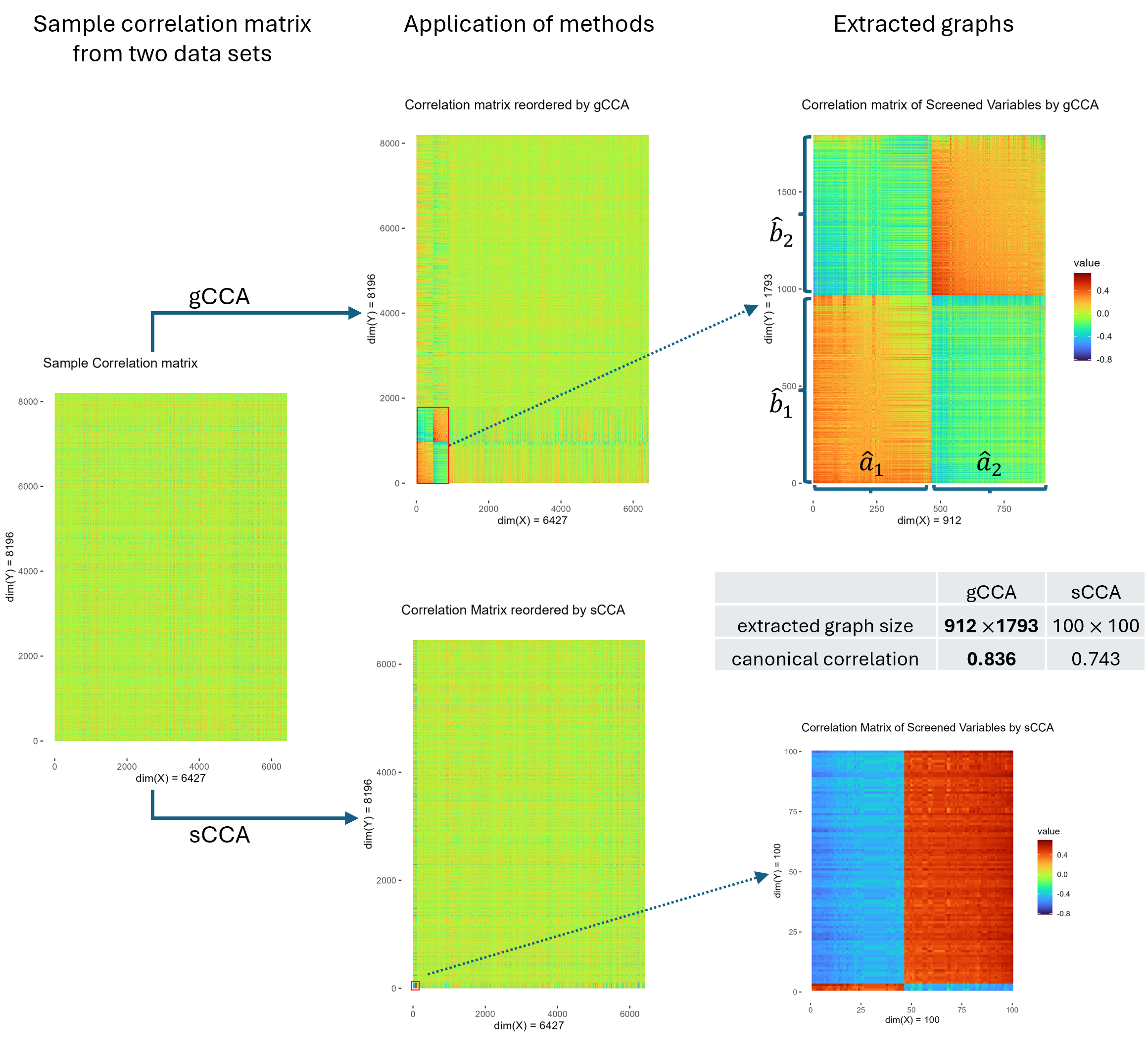
Figure 3: Heatmaps of sample correlation matrices in the realdata analysis. The leftmost one is the sample correlation matrix. The two middle ones are the reordered correlation matrices by gCCA (top) and sCCA (bottom). The two figures on the rightmost are the extracted subgraphs from the TCGA-GBM data set by gCCA (top) and sCCA (bottom), respectively. The subgraphs extracted by gCCA and sCCA are of sizes 912 by 1793 and 100 by 100, respectively, with canonical correlations of 0.836 for gCCA and 0.743 for sCCA.

6 Discussion

We have developed a new graph-based canonical correlation analysis tool - gCCA to decipher the systematic correlations between two sets of high-dimensional variables. Compared to traditional CCA methods, gCCA seeks not only to maximize the correlation between two canonical vectors but also to identify the latent patterns of correlated sets of variables taking the concept of a bipartite graph into account. gCCA can better differentiate the positively and negatively correlated variable sets, and yield canonical correlations to better assess the associations. The signs of canonical correlations are important for many applications like multi-omics data analysis, to reveal whether a set of variables positively/negatively affects the other set of variables.

We provide a computationally efficient solution to implement gCCA with the upper bound of complexity $O((p+q)^{2})$. We also show that the greedy algorithm for gCCA guarantees the full recovery of true related and irrelevant variables for associations between two high-dimensional datasets with a high probability under mild assumptions. In addition, we demonstrate that the greedy algorithm for gCCA has square-root estimation consistency for the canonical correlation estimation. To the best of our knowledge, non-asymptotic analysis of square-root estimation consistency in CCA has not been explored, although some asymptotic analyses have been conducted in this area (Anderson, 1999).

The simulation studies validate our theoretical results by showing that gCCA outperforms conventional methods to more accurately reveal the correlated variables and reduce the estimation bias of the canonical correlation. In our data application, we use gCCA to identify the systematic correlations between two DNA methylation pathways and two RNA expression pathways with both negative and positive correlations, revealing the new interactive biological pathways and their associations using multi-omics data.

Availability and Implementation

The R code that implements gCCA is available at https://github.com/hjpark0820/gCCA.

7 Supplementary Materials

7.1 Proof of the statement in Assumption 3.1 for Gaussian distributions

Let $f_{n}(r|\rho)$ be the density for a sample correlation $R$ of bivariate normal distribution with correlation coefficient $\rho$ and sample size $n>3$. In the work of Hotelling (1953), it is written as follows:

$$f_{n}(r|\rho)=\frac{n-1}{\sqrt{2\pi}}\frac{\Gamma(n)}{\Gamma(n+\frac{1}{2})}(1-\rho^{2})^{\frac{n}{2}}(1-r^{2})^{\frac{n-3}{2}}(1-\rho r)^{-n+\frac{1}{2}}\prescript{~}{2}{F}_{1}\left(\frac{1}{2},\frac{1}{2},n+\frac{1}{2},\frac{1+r\rho}{2}\right),$$

where $\prescript{}{2}{F}_{1}$ is the hypergeometric function such that

$$\prescript{}{2}{F}_{1}(a,b,c,x)=1+\frac{ab}{c}x+\frac{a(a+1)b(b+1)}{2!c(c+1)}x^{2}+\dots,$$

which is convergent for $x\in(-1,1)$. Without loss of generality, we can consider $0\leq\rho<1$ as the argument for the case $\rho<0$ is symmetric for the case $\rho>0$. For $|\rho|=1$, the upper bound is trivial. To find an upper bound of $P(|R-\rho|>\epsilon)$ for $\epsilon\geq 0$, we consider three mutually exclusive cases: (i) $R-\rho>\epsilon$, (ii) $-(R-\rho)<\epsilon$ and $0<\epsilon<\rho$, and (iii) $-(R-\rho)<\epsilon$ and $\rho<\epsilon$. First, we evaluate $P(R-\rho>\epsilon)$ for case (i).

$$P(R-\rho>\epsilon)$$

$$= \int_{\rho+\epsilon}^{1}\frac{n-1}{\sqrt{2\pi}}\frac{\Gamma(n)}{\Gamma(n+\frac{1}{2})}(1-\rho^{2})^{\frac{n}{2}}(1-r^{2})^{\frac{n-3}{2}}(1-\rho r)^{-n+\frac{1}{2}}\prescript{}{2}{F}_{1}\left(\frac{1}{2},\frac{1}{2},n+\frac{1}{2},\frac{1+r\rho}{2}\right)dr$$

$$\leq M_{1}\frac{n-1}{\sqrt{2\pi}}\frac{\Gamma(n)}{\Gamma(n+\frac{1}{2})}\int_{\rho+\epsilon}^{1}(1-\rho^{2})^{\frac{n}{2}}(1-r^{2})^{\frac{n-3}{2}}(1-\rho r)^{-n+\frac{1}{2}}dr$$

where $M_{1}=\sup_{r\in[-1,1]}\prescript{}{2}{F}_{1}(1/2,1/2,n+1/2,\frac{1+r\rho}{2})<\infty$. Note that $\prescript{}{2}{F}_{1}\left(\frac{1}{2},\frac{1}{2},n+\frac{1}{2},\frac{1+r\rho}{2}\right)$ is positive as $0<\frac{1+r\rho}{2}<1$ and $\prescript{}{2}{F}_{1}\left(\frac{1}{2},\frac{1}{2},n+\frac{1}{2},\frac{1+r\rho}{2}\right)\leq\prescript{}{2}{F}_{1}\left(\frac{1}{2},\frac{1}{2},\frac{3}{2},\frac{1+r\rho}{2}\right)=\text{arcsin}\left(\sqrt{\frac{1+r\rho}{2}}\right)/\sqrt{\frac{1+r\rho}{2}}$ (Lozier, 2003). As $\text{arcsin}\left(\sqrt{\frac{1+r\rho}{2}}\right)/\sqrt{\frac{1+r\rho}{2}}$ is continuous in $r\in[-1,1]$, $\prescript{}{2}{F}_{1}\left(\frac{1}{2},\frac{1}{2},\frac{3}{2},\frac{1+r\rho}{2}\right)$ is bounded by a positive constant $M_{1}$.

Using $(a+b)/2\geq\sqrt{ab}$ for $a,b>0$, we have

$$(1-\rho^{2})^{\frac{n-3}{2}}(1-r^{2})^{\frac{n-3}{2}}(1-\rho r)^{-(n-3)} = \left(\left(\frac{1-\rho^{2}}{1-\rho r}\right)^{1/2}\left(\frac{1-r^{2}}{1-\rho r}\right)^{1/2}\right)^{n-3}$$

$$\leq \left(\frac{1}{2}\cdot\frac{(1-\rho^{2})+1-r^{2}}{1-\rho r}\right)^{n-3}$$

$$= \left(1-\frac{1}{2}\cdot\frac{(r-\rho)^{2}}{1-\rho r}\right)^{n-3}.$$

Accordingly, we have

$$\int_{\rho+\epsilon}^{1}(1-\rho^{2})^{\frac{n}{2}}(1-r^{2})^{\frac{n-3}{2}}(1-\rho r)^{-n+\frac{1}{2}}dr$$

$$\leq (1-\rho^{2})^{\frac{3}{2}}(1-\rho)^{-\frac{5}{2}}\int_{\rho+\epsilon}^{1}(1-\rho^{2})^{\frac{n-3}{2}}(1-r^{2})^{\frac{n-3}{2}}(1-\rho r)^{-n+3}dr$$

$$\leq (1-\rho^{2})^{\frac{3}{2}}(1-\rho)^{-\frac{5}{2}}\int_{\rho+\epsilon}^{1}\left(1-\frac{1}{2}\cdot\frac{(r-\rho)^{2}}{1-\rho r}\right)^{n-3}dr$$

Using $1-x\leq e^{-x}$ for $x>0$, for $r>\rho+\epsilon$, we have

$$\left(1-\frac{1}{2}\cdot\frac{(r-\rho)^{2}}{1-\rho r}\right)^{n-3}\leq\exp\left(-\frac{(n-3)(r-\rho)^{2}}{2(1-\rho r)}\right)\leq\exp\left(-\frac{(n-3)(r-\rho)^{2}}{2(1-\rho^{2})}\right).$$

Thus, we have

$$\int_{\rho+\epsilon}^{1}\left(1-\frac{1}{2}\cdot\frac{(r-\rho)^{2}}{1-\rho r}\right)^{n-3}dr\leq\int_{\rho+\epsilon}^{1}\exp\left(-\frac{(n-3)(r-\rho)^{2}}{2(1-\rho^{2})}\right)dr\leq\int_{\epsilon}^{\infty}\exp\left(-\frac{(n-3)r^{2}}{2(1-\rho^{2})}\right)dr.$$

Using the inequality $1-\Phi(z)\leq\exp(-z^{2}/2),~z>0$, where $\Phi(\cdot)$ is the CDF of standard normal distribution, we have

$$1-\Phi\left(\frac{\sqrt{n-3}\epsilon}{\sqrt{1-\rho^{2}}}\right)=\int_{\epsilon}^{\infty}\frac{\sqrt{n-3}}{\sqrt{2\pi(1-\rho^{2})}}\exp\left(-\frac{(n-3)r^{2}}{2(1-\rho^{2})}\right)dr\leq\exp\left(-\frac{(n-3)\epsilon^{2}}{2(1-\rho^{2})}\right).$$

$$P(R-\rho>\epsilon) \leq M_{1}\frac{n-1}{\sqrt{2\pi}}\frac{\Gamma(n)}{\Gamma(n+\frac{1}{2})}\frac{\sqrt{2\pi(1-\rho^{2})}}{\sqrt{n-3}}(1-\rho^{2})^{\frac{3}{2}}(1-\rho)^{-\frac{5}{2}}\exp\left(-\frac{n\epsilon^{2}}{2(1-\rho^{2})}\right)$$ (11)

$$\leq \frac{(n-1)\Gamma(n)}{\sqrt{n-3}\Gamma(n+\frac{1}{2})}(1-\rho^{2})^{2}(1-\rho)^{-\frac{5}{2}}\exp\left(-\frac{(n-3)\epsilon^{2}}{2(1-\rho^{2})}\right)$$

$$\leq M_{1}M_{2}(1+\rho)^{2}(1-\rho)^{-\frac{1}{2}}\exp\left(-\frac{(n-3)\epsilon^{2}}{2(1-\rho^{2})}\right),$$

where $M_{2}=\sup_{n\geq 4}\frac{(n-1)\Gamma(n)}{\sqrt{n-3}\Gamma(n+\frac{1}{2})}$. $M_{2}$ is finite as $\frac{\Gamma(n)}{\Gamma(n+\frac{1}{2})}\leq\sqrt{\frac{1}{n+1/4}}$ (Qi, 2010).

Next, we calculate $P(-(R-\rho)>\epsilon)$ for $0<\epsilon<\rho$ for case (ii). Note that

$$\int_{0}^{\rho-\epsilon}f_{n}(r|\rho)dr$$

$$\leq \int_{0}^{\rho-\epsilon}\frac{n-1}{\sqrt{2\pi}}\frac{\Gamma(n)}{\Gamma(n+\frac{1}{2})}(1-\rho^{2})^{\frac{n}{2}}(1-r^{2})^{\frac{n-3}{2}}(1-\rho r)^{-n+\frac{1}{2}}\prescript{}{2}{F}_{1}\left(\frac{1}{2},\frac{1}{2},n+\frac{1}{2},\frac{1+r\rho}{2}\right)dr.$$

Similarly to the proof for case (i), we have

$$\int_{0}^{\rho-\epsilon}(1-\rho^{2})^{\frac{n}{2}}(1-r^{2})^{\frac{n-3}{2}}(1-\rho r)^{-n+\frac{1}{2}}dr$$

$$\leq (1-\rho^{2})^{\frac{3}{2}}(1-\rho^{2})^{-\frac{5}{2}}\int_{0}^{\rho-\epsilon}(1-\rho^{2})^{\frac{n-3}{2}}(1-r^{2})^{\frac{n-3}{2}}(1-\rho r)^{-n+3}dr$$

$$\leq (1-\rho^{2})^{-1}\int_{0}^{\rho-\epsilon}\left(1-\frac{1}{2}\cdot\frac{(r-\rho)^{2}}{1-\rho r}\right)^{n-3}dr$$

$$\leq (1-\rho^{2})^{-1}\int_{0}^{\rho-\epsilon}\left(1-\frac{1}{2}(r-\rho)^{2}\right)^{n-3}dr$$

$$\leq (1-\rho^{2})^{-1}\int_{0}^{\rho-\epsilon}\exp\left(-\frac{(n-3)(r-\rho)^{2}}{2}\right)dr$$

Accordingly, we have

$$1-\Phi\left(\sqrt{n-3}\epsilon\right)=\int_{-\infty}^{\rho-\epsilon}\frac{\sqrt{n-3}}{\sqrt{2\pi}}\exp\left(-\frac{(n-3)(r-\rho)^{2}}{2}\right)dr\leq\exp\left(-\frac{(n-3)\epsilon^{2}}{2}\right).$$

Thus, we have

$$\int_{0}^{\rho-\epsilon}\frac{n-1}{\sqrt{2\pi}}\frac{\Gamma(n)}{\Gamma(n+\frac{1}{2})}(1-\rho^{2})^{\frac{n}{2}}(1-r^{2})^{\frac{n-3}{2}}(1-\rho r)^{-n+\frac{1}{2}}\prescript{}{2}{F}_{1}\left(\frac{1}{2},\frac{1}{2},n+\frac{1}{2},\frac{1+r\rho}{2}\right)dr$$ (12)

$$\leq M_{1}\frac{n-1}{\sqrt{2\pi}}\frac{\Gamma(n)}{\Gamma(n+\frac{1}{2})}\frac{\sqrt{2\pi}}{\sqrt{n-3}}(1-\rho^{2})^{-1}\exp\left(-\frac{(n-3)\epsilon^{2}}{2}\right)$$

$$\leq M_{1}M_{2}(1-\rho^{2})^{-1}\exp\left(-\frac{(n-3)\epsilon^{2}}{2}\right).$$

Lastly, we calculate $P(R-\rho<-\epsilon)$ for $\rho<\epsilon$. Based on a similar logic to those in the previous two cases, we have

$$\int_{-1}^{\rho-\epsilon}(1-\rho^{2})^{\frac{n}{2}}(1-r^{2})^{\frac{n-3}{2}}(1-\rho r)^{-n+\frac{1}{2}}dr$$

$$\leq (1-\rho^{2})^{\frac{3}{2}}\int_{-1}^{\rho-\epsilon}(1-\rho^{2})^{\frac{n-3}{2}}(1-r^{2})^{\frac{n-3}{2}}(1-\rho r)^{-n+3}dr$$

$$\leq (1-\rho^{2})^{\frac{3}{2}}\int_{-1}^{\rho-\epsilon}\left(1-\frac{1}{2}\cdot\frac{(r-\rho)^{2}}{1-\rho r}\right)^{n-3}dr$$

$$\leq (1-\rho^{2})^{\frac{3}{2}}\int_{-1}^{\rho-\epsilon}\left(1-\frac{(r-\rho)^{2}}{2(1+\rho)}\right)^{n-3}dr$$

$$\leq (1-\rho^{2})^{\frac{3}{2}}\int_{-1}^{\rho-\epsilon}\exp\left(-\frac{(n-3)(r-\rho)^{2}}{2(1+\rho)}\right)dr$$

Accordingly, we have

$$1-\Phi\left(\frac{\sqrt{n-3}\epsilon}{\sqrt{1+\rho}}\right)=\int_{-\infty}^{\rho-\epsilon}\frac{\sqrt{n-3}}{\sqrt{2\pi(1+\rho)}}\exp\left(-\frac{(n-3)(r-\rho)^{2}}{2(1+\rho)}\right)dr\leq\exp\left(-\frac{(n-3)\epsilon^{2}}{2(1+\rho)}\right).$$

Thus, we have

$$\int_{-1}^{\rho-\epsilon}\frac{n-1}{\sqrt{2\pi}}\frac{\Gamma(n)}{\Gamma(n+\frac{1}{2})}(1-\rho^{2})^{\frac{n}{2}}(1-r^{2})^{\frac{n-3}{2}}(1-\rho r)^{-n+\frac{1}{2}}\prescript{}{2}{F}_{1}\left(\frac{1}{2},\frac{1}{2},n+\frac{1}{2},\frac{1+r\rho}{2}\right)dr$$ (13)

$$\leq M_{1}\frac{n-1}{\sqrt{2\pi}}\frac{\Gamma(n)}{\Gamma(n+\frac{1}{2})}\frac{\sqrt{2\pi(1+\rho)}}{\sqrt{n-3}}(1-\rho^{2})^{\frac{3}{2}}\exp\left(-\frac{(n-3)\epsilon^{2}}{2(1+\rho)}\right)$$

$$\leq M_{1}M_{2}(1+\rho)^{\frac{1}{2}}\exp\left(-\frac{(n-3)\epsilon^{2}}{2(1+\rho)}\right).$$

Putting (11), (12), and (13) all together, we have

$$P(|R-\rho|>\epsilon)\leq 2M_{1}M_{2}(1-\rho)^{-1}\exp\left(-\frac{(n-3)\epsilon^{2}}{2(1+\rho)}\right).$$

Therefore, there exist $s_{1}>0$ and $s_{2}>0$ such that

$$P(|R-\rho|>\epsilon)\leq s_{1}\exp\left(-\frac{n\epsilon^{2}}{2s_{2}}\right).$$

7.2 Proof of the equivalence of Assumption 3.1 to $E[e^{\lambda(R_{ij}-\theta_{ij})}]\leq s_{3}e^{s_{4}^{2}\lambda^{2}/n}$

Let $X=\sqrt{n}(R_{ij}-\theta_{ij})/(\sqrt{2}s_{2})$ for ease of presentation. Then, we have

$$E\left[\left|X\right|^{p}\right] = \int_{0}^{\infty}P(|X|^{p}\geq u)du$$

$$= \int_{0}^{\infty}P(|X|\geq t)pt^{p-1}dt$$

$$\leq \int_{0}^{\infty}s_{1}e^{-t^{2}}pt^{p-1}dt.$$

By letting $t^{2}=s$ and then using the definition of the Gamma function, we have

$$\int_{0}^{\infty}s_{1}e^{-t^{2}}pt^{p-1}dt = (s_{1}/2)p\Gamma(p/2).$$

Then, with the Stirling approximation $\Gamma(x)\leq x^{x}$, we get

$$E\left[\left|X\right|^{p}\right]\leq(s_{1}/2)(p/2)^{p/2}.$$

Using $Ee^{\lambda^{2}X^{2}}=E(1+\sum_{p=1}^{\infty}\frac{(\lambda^{2}X^{2})^{p}}{p!})\leq 1+\sum_{p=1}^{\infty}\frac{\lambda^{2p}E[X^{2p}]}{p!}$ and $p!\geq(p/e)^{p}$, we have

$$Ee^{\lambda^{2}X^{2}}\leq 1+\sum_{p=1}^{\infty}\frac{(s_{1}/2)(2\lambda^{2}p)^{p}}{(p/2)^{p}}\leq\frac{s_{1}}{2}\sum_{p=0}^{\infty}(2e\lambda^{2})^{p}=\frac{s_{1}}{2}\cdot\frac{1}{1-2e\lambda^{2}},$$

provided that $2e\lambda^{2}<1$. Using $1/(1-x)\leq e^{2x}$ for $x\in[0,1/2]$, we have

$$Ee^{\lambda^{2}X^{2}}\leq\frac{s_{1}}{2}e^{4e\lambda^{2}},~|\lambda|\leq\frac{1}{\sqrt{2e}}.$$

Now, we focus on $Ee^{\lambda X}$. For $|\lambda|\leq 1$, using $e^{x}\leq x+e^{x^{2}}$ and $E[X]=0$, we have

$$Ee^{\lambda X}\leq E(\lambda X+e^{\lambda^{2}X^{2}})=Ee^{\lambda^{2}X^{2}}\leq\frac{s_{1}}{2}e^{4e\lambda^{2}}.$$

Next, we prove the case with $|\lambda|\geq 1$. Using $2\lambda x\leq\lambda^{2}+x^{2}$, we have

$$Ee^{\lambda X}\leq e^{\lambda^{2}/2}Ee^{X^{2}/2}\leq(s_{1}/2)e^{\lambda^{2}/2}e^{2e}\leq(s_{1}/2)e^{2e}e^{\lambda^{2}},~~~\text{for}~|\lambda|\geq 1.$$

Putting the two cases $|\lambda|\leq 1$ and $|\lambda|\geq 1$ together, for $\lambda\in\mathbb{R}^{1}$, we have

$$Ee^{\lambda X}\leq(s_{1}/2)e^{2e}e^{4e\lambda^{2}}.$$

Letting $X=\sqrt{n}(R_{ij}-\theta_{ij})/(\sqrt{2}s_{2})$, we have

$$Ee^{\lambda(R_{ij}-\theta_{ij})}\leq(s_{1}/2)e^{2e}e^{2es_{2}^{2}\lambda^{2}/n}.$$

Thus, by defining $s_{3}=(s_{1}/2)e^{2e}$ and $s_{4}^{2}=2es_{2}^{2}$, we have

$$Ee^{\lambda(R_{ij}-\theta_{ij})}\leq s_{3}e^{s_{4}^{2}\lambda^{2}/n}.$$ (14)

Now, we show that there exist $s_{1},s_{2}>0$ such that $P(|R_{ij}-\theta_{ij}|>t)\leq s_{1}\exp(-\frac{t^{2}}{2s_{2}^{2}})$, if (14) is true. Note that

$$P(R_{ij}-\theta_{ij}\geq t)=P(e^{\lambda(R_{ij}-\theta_{ij})}\geq e^{\lambda t})\leq e^{-\lambda t}Ee^{\lambda(R_{ij}-\theta_{ij})}\leq e^{-\lambda t}s_{3}e^{s_{4}^{2}\lambda^{2}}=s_{3}e^{-\lambda t+s_{4}^{2}\lambda^{2}}.$$

Thus, by letting $\lambda=t/2s_{4}^{2}$, we have

$$P(R_{ij}-\theta_{ij}\geq t)\leq s_{3}e^{-t^{2}/4s_{4}^{2}}.$$

We can get the same result for $P(R_{ij}-\theta_{ij}<-t)$ for $t<0$ with the same logic. Therefore, we have

$$P(|R_{ij}-\theta_{ij}|\geq t)\leq 2s_{3}e^{-nt^{2}/4s_{4}^{2}}.$$

7.3 Proof of the statement in Assumption 3.1 for Gaussian distributions

Let ${\bf X}_{i}=(X_{i1},X_{i2},\dots,X_{in})^{\top}$ be a random vector such that each $X_{ij}$ is independently generated from $N(\mu_{i},\sigma_{i}^{2})$. We assume that ${\bf X}_{1}$, ${\bf X}_{2}$, and ${\bf X}_{3}$ are mutually independent. We let centered and standardized vectors of ${\bf X}_{i}$, ${\bf X}_{2}$, and ${\bf X}_{3}$, with sample size $n$, denoted by ${\bf Y}_{1}$, ${\bf Y}_{2}$, and ${\bf Y}_{3}$, respectively. Since they are centered and standardized, they are in $\mathbb{S}^{d-1}$. In addition, $R_{ij}={\bf Y}_{i}^{\top}{\bf Y}_{j}$. Because each random variable ${\bf X}_{i}$ is independent from each other, ${\bf Y}_{i}$ is unformly distributed in $\mathbb{S}^{d-1}$. Consider the joint density of ${\bf Y}_{1}$ and $R_{12}=r_{12}$. Then, we have

$$f({\bf Y}_{1}=y_{1},R_{12}=r_{12})=f(R_{12}=r_{12}|{\bf Y}_{1}=y_{1})f({\bf Y}_{1}=y_{1}).$$

Here, note that $R_{12}=r_{12}$ represents ${\bf Y}_{2}^{\top}y_{1}=r_{12}$ and that $r_{12}$ represents $\text{cos}(\theta_{12})$, where $\theta_{12}$ is the angle between ${\bf Y}_{1}$ and ${\bf Y}_{2}$. The set $\{y:y^{\top}y_{1}=r_{12}\}\in\mathbb{S}^{d-1}$ is the collection of vectors in $\mathbb{S}^{d-1}$ that have the angle $\theta_{12}=\text{cos}^{-1}(r_{12})$ with $y_{1}$. Since ${\bf Y}_{2}$ is independent of ${\bf Y}_{1}$ and uniformly distributed over $\mathbb{S}^{d-1}$, the probability density of $\{y:y^{\top}y_{1}=r_{12}\}$ does not depend on the value of $y_{1}$. This means

$$f(R_{12}=r_{12}|{\bf Y}_{1}=y_{1})=f(R_{12}=r_{12}).$$

Accordingly, we have

$$f({\bf Y}_{1}=y_{1},R_{12}=r_{12})=f(R_{12}=r_{12})f({\bf Y}_{1}=y_{1}).$$

Thus, ${\bf Y}_{1}$ and $R_{12}$ are indenpendent. Because ${\bf Y}_{3}$ is also independent from $R_{12}$, $R_{13}={\bf Y}_{1}^{\top}{\bf Y}_{3}$ and $R_{12}$ are independent. Therefore, Assumption 3.1 holds for normal distributions.

7.4 Proof of Lemma 3.1

Proof 7.1

Let $\frac{\delta}{pq}=s_{1}\exp(-na^{2}/2s_{2}^{2})$ in Assumption 3.1. Then, we have $P\left(|R_{ij}-\rho_{ij}|>\sqrt{\frac{2s_{2}^{2}}{n}\log\left(\frac{s_{1}pq}{\delta}\right)}\right)\leq\frac{\delta}{pq}$. Thus, we have

$$P\left(|R_{ij}-\rho_{ij}|>\sqrt{\frac{2s_{2}^{2}}{n}\log\left(\frac{s_{1}pq}{\delta}\right)},~\text{for~all}~(i,j)\in[p]\otimes[q]\right)\leq pq\frac{\delta}{pq}=\delta.$$

7.5 Proof of Lemma 3.2

Proof 7.2

By Lemma 3.1, for all $i$ and $j$, we have $|R_{ij}-\rho_{ij}|<\sqrt{\frac{2s_{2}^{2}}{n}\log\left(\frac{s_{1}pq}{\delta}\right)}$ with probability at least $1-\delta$. If $n\geq(\eta/\rho)^{2}(2s_{2}^{2}\log\left(s_{1}pq/\delta\right))$, we have $\sqrt{\frac{2s_{2}^{2}}{n}\log\left(\frac{s_{1}pq}{\delta}\right)}<\rho/\eta.$ Accordingly, we have $|R_{ij}|>\frac{\eta-1}{\eta}\rho$ for $i\in I_{X}~\text{and}~j\in I_{Y}$ and $|R_{ij}|<\frac{1}{\eta}\rho$ for $i\in I_{X}^{c}~\text{or}~j\in I_{Y}^{c}$. Now, we consider $|R_{ij}^{\varepsilon}|$ for $0\leq\varepsilon<\rho/2$. As $\frac{\eta-1}{\eta}\rho>\varepsilon$ and $|R_{ij}|\geq|R_{ij}^{\varepsilon}|$, we still have

$$|R_{ij}^{\varepsilon}|>\frac{\eta-1}{\eta}\rho,~~~\text{for}~i\in I_{X}~\text{and}~j\in I_{Y}$$ (15)

and

$$|R_{i^{\prime}j}^{\varepsilon}|<\frac{1}{\eta}\rho,~~~\text{for}~i^{\prime}\in I_{X}^{c}~\text{or}~j\in I_{Y}^{c}.$$ (16)

Thus, we have $\sum_{j\in I_{Y}}|R_{ij}^{\varepsilon}|>q_{0}((\eta-1)/\eta)\rho$ for all $i\in I_{X}$ and $\sum_{j\in I_{Y}}|R_{i^{\prime}j}^{\varepsilon}|<q_{0}(\rho/\eta)$ for all $i^{\prime}\in I_{X}^{c}$ with probability at least $1-\delta$. Accordingly, we have $\sum_{j\in I_{Y}}(|R_{ij}^{\varepsilon}|-|R_{i^{\prime}j}^{\varepsilon}|)>q_{0}\rho(\eta-2)/\eta$ for $i\in I_{X}$ and $i^{\prime}\in I_{X}^{c}$ with probability at least $1-\delta$. In the same way, we can show $\sum_{i\in I_{X}}(|R_{ij}^{\varepsilon}|-|R_{ij^{\prime}}^{\varepsilon}|)>p_{0}\rho(\eta-2)/\eta$ for $j\in I_{Y}$ and $j^{\prime}\in I_{Y}^{c}$ with probability at least $1-\delta$.

7.6 Proof of Lemma 3.3

Proof 7.3

Assumption 3.1 is applicable to $(i_{1},h_{1}(t))$ and $(i_{2},h_{1}(t))$ for all $t\in[q-q_{0}]$, as $(i_{1},h_{1}(t))$ and $(i_{2},h_{1}(t))$ are not in the subgraph for all $t\in[q-q_{0}]$. Consequently, based on Assumption 3.1, for all $a>0$, we have

$$E\left[e^{a(|R_{i_{1}h_{1}(t)}^{\varepsilon}|-|R_{i_{1}h_{1}(t)}^{\varepsilon}|)}\right]=E\left[e^{a|R_{i_{1}h_{1}(t)}^{\varepsilon}|}\right]E\left[e^{-a|R_{i_{1}h_{1}(t)}^{\varepsilon}|}\right]\leq s_{3}e^{\frac{s_{4}^{2}a^{2}}{n}}.$$

Letting $a=\sqrt{n/s_{4}^{2}}$, we have

$$E\left[e^{\sqrt{\frac{n}{s_{4}^{2}}}(|R_{i_{1}h_{1}(t)}^{\varepsilon}|-|R_{i_{1}h_{1}(t)}^{\varepsilon}|)}\right]\leq s_{3}e.$$

For $i_{1},i_{2}\in[p]$, let

$$M_{t}^{i_{1}i_{2}}=\exp\left(\sqrt{\frac{n}{s_{4}^{2}}}\sum_{j=1}^{t}(|R_{i_{1}h_{1}(j)}^{\varepsilon}|-|R_{i_{2}h_{1}(j)}^{\varepsilon}|)-(1+\log s_{3})t\right)$$

where $M_{t}^{i_{1}i_{2}}=M_{q-q_{0}}^{i_{1}i_{2}}$ for $t\geq q-q_{0}$ and $\tau$ be a stopping time with respect to the filtration $\{\mathcal{F}_{t-1}^{i_{1}i_{2}}\}_{t}$, where $\mathcal{F}_{t}^{i_{1}i_{2}}=\sigma\{\{|R_{i_{1}h_{1}(j)}^{\varepsilon}|,|R_{i_{2}h_{1}(j)}^{\varepsilon}|\}_{j=1}^{t}\}$. First, we claim $\{M_{t}^{i_{1}i_{2}}\}_{t=1}^{q-q_{0}}$ is a supermartingale. Let $D_{t}^{i_{1}i_{2}}=\exp\left(\sqrt{\frac{n}{s_{4}^{2}}}(|R_{i_{1}h_{1}(t)}^{\varepsilon}|-|R_{i_{2}h_{1}(t)}^{\varepsilon}|)-(1+\log s_{3})\right)$. By Assumption 3.1, $D_{t}^{i_{1}i_{2}}$ and $\mathcal{F}_{t-1}^{i_{1}i_{2}}$ are independent. Thus, we have

$$E[D_{t}^{i_{1}i_{2}}|\mathcal{F}_{t-1}^{i_{1}i_{2}}]\leq E\left[e^{\sqrt{\frac{n}{s_{4}^{2}}}(|R_{i_{1}h_{1}(t)}^{\varepsilon}|-(1+\log s_{3}))}\right]\leq 1.$$

Clearly, $D_{t}^{i_{1}i_{2}}$ is $\mathcal{F}_{t}^{i_{1}i_{2}}$-measurable, as is $M_{t}^{i_{1}i_{2}}$. Further, we have $E[M_{t}^{i_{1}i_{2}}|\mathcal{F}_{t-1}^{i_{1}i_{2}}]=D_{1}^{i_{1}i_{2}}\cdots D_{t-1}^{i_{1}i_{2}}E[D_{t}^{i_{1}i_{2}}|\mathcal{F}_{t-1}^{i_{1}i_{2}}]\leq M_{t-1}^{i_{1}i_{2}}$. This shows that $\{M_{t}^{i_{1}i_{2}}\}$ is a supermartingale. By the convergence theorem for nonnegative supermartingales (Doob, 1953), $M_{\infty}^{i_{1}i_{2}}=\lim_{t\rightarrow\infty}M_{t}^{i_{1}i_{2}}$ is almost surely well-defined. Hence, $M_{\tau}^{i_{1}i_{2}}$ is well-defined. Next, let $Q_{t}^{i_{1}i_{2}}=M_{\min(\tau,t)}^{i_{1}i_{2}}$ be a stopped version of $\{M_{t}^{i_{1}i_{2}}\}$. By Fatou’s lemma (Rudin et al., 1976), we have

$$E[\text{liminf}_{t\rightarrow\infty}Q_{t}^{i_{1}i_{2}}]\leq\text{liminf}_{t\rightarrow\infty}E[Q_{t}^{i_{1}i_{2}}]\leq 1.$$

This shows that $E[M_{\tau}^{i_{1}i_{2}}]\leq 1$ holds. Lastly, from $E[M_{\tau}^{i_{1}i_{2}}]\leq 1$, we get

$$P\left(\sqrt{\frac{n}{s_{4}^{2}}}\sum_{j=1}^{\tau}(|R_{i_{1}h_{1}(j)}^{\varepsilon}|-|R_{i_{2}h_{1}(j)}^{\varepsilon}|)-\tau(1+\log s_{3})>\log\delta^{-1}\right)=P\left(M_{\tau}^{i_{1}i_{2}}\delta^{-1}>1\right)$$

$$\leq E[M_{\tau}^{i_{1}i_{2}}\delta]\leq\delta.$$

In other words, we have

$$\sqrt{\frac{n}{s_{4}^{2}}}\sum_{j=1}^{\tau}(|R_{i_{1}h_{1}(j)}^{\varepsilon}|-|R_{i_{2}h_{1}(j)}^{\varepsilon}|)-\tau(1+\log s_{3})>\log\delta^{-1}$$

with probability at least $1-\delta$. Similarly, for $j_{1}\in I_{Y}$ and $j_{2}\in I_{Y}^{c}$, we have

$$\sqrt{\frac{n}{s_{4}^{2}}}\sum_{t=1}^{\tau}(|R_{h_{2}(t)j_{1}}^{\varepsilon}|-|R_{h_{2}(t)j_{2}}^{\varepsilon}|)-\tau(1+\log s_{3})>\log\delta^{-1}$$

with probability at least $1-\delta$, where $h_{2}$ is a bijective function from $\{1,2,\dots,p-p_{0}\}$ to $I_{X}^{c}$. By plugging $\frac{\delta}{2\max(p,q)^{2}}$ into $\delta$, if $n>\frac{\eta^{2}s_{4}^{2}}{2\min(p_{0},q_{0})^{2}(\eta-2)^{2}\rho^{2}}\left(\max(p,q)(1+\log s_{3})+\log\frac{2\max(p,q)^{2}}{\delta}\right)^{2}$, we have

$$\sum_{t=1}^{\tau}(|R_{i_{1}h_{1}(t)}^{\varepsilon}|-|R_{i_{2}h_{1}(t)}^{\varepsilon}|)\leq\frac{\min(p_{0},q_{0})(\eta-2)\rho}{\eta},$$

for all $i_{1}\in I_{X}$ and all $i_{2}\in I_{X}^{c}$ and

$$\sum_{t=1}^{\tau}(|R_{h_{2}(t)j_{1}}^{\varepsilon}|-|R_{h_{2}(t)j_{2}}^{\varepsilon}|)\leq\frac{\min(p_{0},q_{0})(\eta-2)\rho}{\eta},$$

for all $j_{1}\in I_{Y}$ and all $j_{2}\in I_{Y}^{c}$ with probability at least $1-\delta$.

References

• Anderson (1999) Anderson, T. W. (1999). Asymptotic theory for canonical correlation analysis. Journal of Multivariate Analysis 70, 1–29.
• Bertsimas et al. (2016) Bertsimas, D., King, A., and Mazumder, R. (2016). Best subset selection via a modern optimization lens.
• Boucheron et al. (2003) Boucheron, S., Lugosi, G., and Bousquet, O. (2003). Concentration inequalities. In Summer school on machine learning, pages 208–240. Springer.
• Bühlmann and Van De Geer (2011) Bühlmann, P. and Van De Geer, S. (2011). Statistics for high-dimensional data: methods, theory and applications. Springer Science & Business Media.
• Charikar (2000) Charikar, M. (2000). Greedy approximation algorithms for finding dense components in a graph. In International workshop on approximation algorithms for combinatorial optimization, pages 84–95. Springer.
• Doob (1953) Doob, J. L. (1953). Stochastic processes, volume 10. New York Wiley.
• Giordano (2014) Giordano, T. J. (2014). The cancer genome atlas research network: a sight to behold. Endocrine Pathology 25, 362–365.
• Hotelling (1936) Hotelling, H. (1936). Relations between two sets of variates. Biometrika pages 321–377.
• Hotelling (1953) Hotelling, H. (1953). New light on the correlation coefficient and its transforms. Journal of the Royal Statistical Society. Series B (Methodological) 15, 193–232.
• Lê Cao et al. (2009) Lê Cao, K.-A., González, I., and Déjean, S. (2009). integromics: an r package to unravel relationships between two omics datasets. Bioinformatics 25, 2855–2856.
• Lee et al. (2024) Lee, H., Ma, T., Ke, H., Ye, Z., and Chen, S. (2024). dcca: detecting differential covariation patterns between two types of high-throughput omics data. Briefings in Bioinformatics 25,.
• Lozier (2003) Lozier, D. W. (2003). Nist digital library of mathematical functions. Annals of Mathematics and Artificial Intelligence 38, 105–119.
• Martinez et al. (2009) Martinez, R., Martin-Subero, J. I., Rohde, V., Kirsch, M., Alaminos, M., Fernandez, A. F., Ropero, S., Schackert, G., and Esteller, M. (2009). A microarray-based dna methylation study of glioblastoma multiforme. Epigenetics 4, 255–264.
• Murphy (2023) Murphy, K. P. (2023). Probabilistic Machine Learning: Advanced Topics. MIT Press.
• Natarajan (1995) Natarajan, B. K. (1995). Sparse approximate solutions to linear systems. SIAM journal on computing 24, 227–234.
• Qi (2010) Qi, F. (2010). Bounds for the ratio of two gamma functions. Journal of Inequalities and Applications 2010, 1–84.
• Rudin et al. (1976) Rudin, W. et al. (1976). Principles of mathematical analysis, volume 3. McGraw-hill New York.
• Tenenhaus et al. (2014) Tenenhaus, A., Philippe, C., Guillemot, V., Le Cao, K.-A., Grill, J., and Frouin, V. (2014). Variable selection for generalized canonical correlation analysis. Biostatistics 15, 569–583.
• Tomczak et al. (2014) Tomczak, K., Czerwińska, P., and Wiznerowicz, M. (2014). The cancer genome atlas (tcga): An immeasurable source of knowledge. wspolczesna onkol. 2015; 1a: A68–a77.
• Vershynin (2018) Vershynin, R. (2018). High-dimensional probability: An introduction with applications in data science, volume 47. Cambridge university press.
• Witten et al. (2009) Witten, D. M., Tibshirani, R., and Hastie, T. (2009). A penalized matrix decomposition, with applications to sparse principal components and canonical correlation analysis. Biostatistics 10, 515–534.
• Witten and Tibshirani (2009) Witten, D. M. and Tibshirani, R. J. (2009). Extensions of sparse canonical correlation analysis with applications to genomic data. Statistical applications in genetics and molecular biology 8,.
• Yang et al. (2019) Yang, X., Liu, W., Liu, W., and Tao, D. (2019). A survey on canonical correlation analysis. IEEE Transactions on Knowledge and Data Engineering 33, 2349–2368.
• Zhou et al. (2024) Zhou, Z., Ataee Tarzanagh, D., Hou, B., Tong, B., Xu, J., Feng, Y., Long, Q., and Shen, L. (2024). Fair canonical correlation analysis. Advances in Neural Information Processing Systems 36,.
• Zhuang et al. (2020) Zhuang, X., Yang, Z., and Cordes, D. (2020). A technical review of canonical correlation analysis for neuroscience applications. Human brain mapping 41, 3807–3833.