Topological variability modes of the wind-driven ocean circulation

Abstract

The wind-driven ocean circulation comprises the oceanic currents that are visible at the surface. In this paper, we use algebraic topology concepts and methods to study a highly simplified model of the evolution of this circulation subject to periodic winds. The low-order spectral model corresponds to a midlatitude ocean basin. For steady forcing, the model’s intrinsic oscillations undergo a bifurcation from small-amplitude harmonic ones to relaxation oscillations (ROs) of high amplitude as the forcing increases. The ROs, in turn, give rise to chaotic behavior under periodic forcing. Topological invariants help identify distinct flow regimes that ensemble simulations visit under the action of the underlying deterministic rule in such a nonautonomous framework. We introduce topological variability modes of this idealized ocean circulation, based on the previously defined invariants.

The theory of nonautonomous dynamical systems (NDSs) provides an appropriate framework for studying how a system’s internal variability responds to changes in external forcing. Henri Poincaré pioneered the application of algebraic topology in dynamics, emphasizing qualitative analysis through homeomorphisms. Classical bifurcations disrupt phase space continuity, rendering a system’s pre- and post-bifurcation state non-homeomorphic. Algebraic topology helps characterize such qualitative changes, even when both states are chaotic. This study demonstrates how a templex reveals the mechanisms underlying different types of chaos within a deterministic framework and how these mechanisms can undergo transformations. The templex combines a cell complex from homology theory — to describe the system’s topological structure in phase space — with a directed graph (digraph) defined on the complex, to describe the flow on that structure. Both the cell complex and the digraph remain invariant in autonomous dynamics but change when the system’s forcing or coefficients change in time. Our results show how the templex captures in a parsimonious manner the qualitative evolution of the wind-driven circulation under periodic forcing.

I Introduction and motivation

Studying intrinsic low-frequency variability of the mid-latitude double-gyre circulation is crucial for understanding ocean dynamics and climate variability in general. Simplified, conceptual models play an important role in identifying the nonlinear processes that are responsible for distinct flow regimes and the transitions between them. The effects of time-dependent forcing on intrinsic ocean variability has been investigated using a full hierarchy of oceanic and coupled ocean-atmosphere models, from the simplest conceptual ones to the highest resolution ones Ghil and Lucarini (2020).

I.1 Simple models of the wind-driven circulation

Idealized models of the wind-driven circulation that emphasize nonlinear effects and the bifurcations they give rise to include the four-dimensional (4-D), spectral quasi-geostrophic (QG) model of Veronis1963, who found periodic solutions, and the spatially two-dimensional (2-D) shallow-water model of Jiang, Jin, and Ghil1995, who studied a finite-difference version thereof that had intermediate horizontal resolution, and found multiple steady states, as well as limit cycles and chaotic solutions. The latter authors also investigated a QG, spectrally 2-D version of their model, in which the western boundary currents Ghil and Childress (2012), absent in earlier work, were introduced by an exponential term in the basis functions.

Simonnet, Ghil, and Dijkstra2005 and Pierini2011 both studied 4-D spectral QG models using the westward intensification of the flow introduced in ref Jiang, Jin, and Ghil (1995), but differed in the selection of their basis functions: the former used the tensor product of one longitudinal mode with four meridional ones, while the latter used the tensor product of two longitudinal and two meridional modes. Simonnet, Ghil, and Dijkstra emphasized the role of a homoclinic bifurcation in finding two types of chaos, of Lorenz1963 type and of Shilnikov1965 type, while Pierini emphasized the role relaxation oscillations (ROs) play in giving rise to chaos, while Pierini, Ghil, and Chekroun2016 went further in exploring the role of time-dependent forcing in affecting the model’s intrinsic chaos.

The model’s four ordinary differential equations form a nonlinear dynamical system for the amplitudes of the flow’s streamfunction modes. Reasonably realistic values for the spatial scales and the wind stress curl can be used, allowing for the expected bifurcation scenario to occur in spite of the severe truncation. The autonomous case was studied for increasing values of the wind stress, yielding steady states, periodic solutions and chaotic ones Pierini (2011); Pierini, Ghil, and Chekroun (2016), including Shilnikov type chaos, in which the homoclinic orbit spirals back to the unstable fixed point. Pierini, Ghil, and Chekroun2016 considered the nonautonomous case for an aperiodic forcing with a decadal characteristic time, while Pierini2014 and Pierini, Chekroun, and Ghil2018 studied the model’s response to periodic forcing by metric methods that did not appeal to algebraic topology.

The purpose of the present paper is to bring to bear on this simple oceanic model recent concepts and methods from the theory of nonautonomous dynamical systems (NDSs) and algebraic topology Ghil and Sciamarella (2023), leading up to the introduction of topological variability modes (TVMs). These TVMs will be shown to be totally different from various other data-driven decomposition modes that are either purely statistical or borrow only moderately from the underlying dynamics, such as empirical orthogonal functions and principal component analysis Preisendorfer (1988); Jolliffe (2002) or proper orthogonal decomposition Berkooz, Holmes, and Lumley (1993).

I.2 Nonutonomous dynamical systems

NDS theory deals with the ways that dynamical systems with time-dependent forcing or coefficients can be handled as completely as autonomous systems in which no time dependence is explicitly built in. For the latter ones, solutions $x(t;t_{0})$ depend only on the elapsed time $t-t_{0}$ between the fixed initial time $t_{0}$ and the time of observation $t$. For NDSs, solutions depend separately, as a two-parameter family, on the initial time usually denoted by $s$ and the time of observation $t$.

For autonomous systems, the only attractors are forward attractors, obtained as $t\to+\infty$. For NDSs, one has either pullback attractors (PBAs), obtained for a given $t$ as $s\to-\infty$, or forward attractors, which we will label as FWAs, obtained for a given $s$ as $t\to+\infty$. The latter though are distinct from the forward attractors of autonomous systems, since the conditions for the existence and uniqueness of an FWA are more complicated Caraballo and Han (2017); Kloeden and Yang (2020). In the mathematical literature, PBAs were introduced first for random dynamical systems by Crauel and Flandoli1994 and by Arnold1988; they were applied to climate problems first by Ghil, Chekroun, and Simonnet2008 and by Chekroun, Simonnet, and Ghil2011.

At roughly the same time, in the physical literature, attractors for NDSs were proposed under the name of snapshot attractors by Namenson, Ott, and Antonsen1996. While these attractors were defined somewat more loosely than the FWAs in the mathematical literature, the two are similar in spirit and Bódai and Tél2012, and Tél et al.2020 used the snapshot attractor name in climate applications. It turns out that, when they exist, snapshot attractors are easier to compute than PBAs, and we will use this name here.

I.3 Algebraic topology and dynamics: the cell complex

As Henri Poincaré observed in 1892 Poincaré (1893), perturbation theory fails to account for the mechanisms of stretching and squeezing of the flow in phase space under the action of deterministic governing equations. This observation led him to lay the foundations of Analysis Situs Poincaré (1895), which has become central to identifying the essential features that distinguish different types of dynamics in phase space. The computation of topology in phase space can be achieved not only through the analysis of point clouds derived from numerical simulations with varying initial conditions but also by reconstructing phase space from observed or measured time series data.

Recent work demonstrates that algebraic topology can characterize chaotic attractors in both autonomous and nonautonomous settings, within deterministic as well as stochastic frameworks Charó et al. (2021); Ghil and Sciamarella (2023), by using Branched Manifold Analysis through Homologies to construct a BraMAH cell complex Sciamarella and Mindlin (1999, 2001) in the autonomous case — or families of cell complexes, if the point cloud representing the attractor at time $t$ evolves over time, in the NDS case. In algebraic topology, a cell complex is a structure composed of cells of various dimensions — e.g., points are 0-cells, segments are 1-cells, polygons are 2-cells, polyhedra are 3-cells, and so on — that can be built from a point cloud to approximate its shape.

Once the cell complex is constructed, it is analyzed algebraically, focusing not on the specific coordinates of the 0-cells but on the way the cells of the complex are glued together Munkres (2018). The algebraic analysis of a BraMAH complex is independent of the particular cell complex used to approximate the point cloud: the cell complex acts as a Wittgenstein ladder Wittgenstein (1922), discarded once the topological properties of the point cloud are identified. These topological properties remain invariant and unaffected by the number, distribution, or size of the cells used to approximate the manifold in which the dataset is embedded.

I.4 Flow on the cell complex and the templex

The point cloud under analysis may be derived from an embedding in phase space of a time series or derived from a trajectory in the full phase space. In either case, the cells of the complex are visited by the trajectory in an order determined by the flow. This order is entirely different from the orientation of the cells as defined in algebraic topology. Cell orientation serves to define an algebra of chains, enabling the computation of homology groups, which represent holes of various dimensions.

In contrast, the sequence in which a trajectory associated with a dynamical system visits the cells is limited to the highest-dimensional cells of the complex, and the possibility of flowing from one cell to another is related to causality. This information can be incorporated using a directed graph (digraph), where the nodes correspond to the highest-dimensional cells of the complex and the edges stand for the connections between cells established by the flow. Together, the cell complex and this digraph form what Charó, Letellier, and Sciamarella2022 called a templex. A templex encodes the topological structure underlying the point cloud, along with the organization of the flow within that structure.

In a random attractor Chekroun, Simonnet, and Ghil (2011), the nature of the point cloud changes: instead of a single point cloud, there exists a sequence of point clouds, one for each snapshot in time. Consequently, Charó, Ghil, and Sciamarella2023 constructed a family of cell complexes, one for each snapshot. They then defined a random templex to track the evolution of the holes over time, from complex to complex. In this setting, the nodes of the digraph represent the generators of the homology groups, while its directed edges indicate the correspondence between holes from one snapshot to the next Charó, Ghil, and Sciamarella (2023).

I.5 Constructing a templex for the problem at hand

An intermediate situation between an autonomous deterministic attractor and a random attractor arises when an autonomous system is subjected to a driving force in a deterministic setting. In such a case, one wishes to understand how the driving force affects the way the flow maps onto itself under the nonautonomous governing equations. How is the topological structure affected? Does forcing only alter the properties of the digraph, or does it also induce changes in the cell complex? How do the ensemble simulations that correspond to the FWA explore the templex? To address these questions, we construct herein templexes for a steady and a periodically forced model of low-frequency variability in the wind-driven ocean circulation.

The article is organized as follows. Section II introduces the main concepts and tools of chaos topology, to prepare for a topological analysis using the templex approach. Section III.1 presents the templex analysis of the four-dimensional autonomous system associated with our low-order spectral QG model. Section III.2 discusses the nonautonomous case, in which a periodic forcing is applied to the model and the corresponding templex analysis is carried out.

In Section IV, we compute the snapshot attractors for the nonautonomous case, and in Section V we introduce and compute the model’s topological variability modes. The conclusions of this study are presented in the final section.

II Chaos topology and the templex approach

The structure of a dynamical system’s flow in phase space emerges from a series of processes — stretching, folding, tearing, and squeezing — that are driven by the governing equations and repeatedly occur for any initial condition Gilmore (2013). This section presents newly developed tools that characterize the topological structure of a deterministic flow in phase space Sciamarella and Charó (2024).

II.1 The cell complex and homology groups

The analysis starts with a point cloud in the full phase space of dimension $n$ or in a lower-dimensional phase space, as long as the subspace is free of false neighbors so as to preserve the topology To compute the topology of the manifold in which the points lie, this point cloud must be (i) sufficiently well-sampled, and (ii) have a long enough time span for the attractor to be completely explored. Grouping subsets of points into cells is the first step in the construction of a cell complex. The subset of points in a cell should be locally homeomorphic to either a full or half disk in $d\leq n$ dimensions, where $d$ is the local dimension of the subset. The cell representing such a subset is termed a $d$-cell.

Let $\bm{\phi}$ represent a sufficiently well sampled flow with an underlying $d$-dimensional manifold in $\mathbb{R}^{n}$. A BraMAH complex of dimension $d$ consists of $k$-cells with $k\leq d$ such that:

1. The $0$-cells form a sparse subset of the original point cloud in phase space;

2. $d\leq n$ denotes the local dimension of the branched manifold; and

3. Each $d$-cell is defined so that $d$ of the singular values characterizing the distribution of points around the barycenter of the $d$-cell scale linearly with the number of points within the cell.

The third property fails to be valid when the local curvature of the branched manifold becomes significant. In this case, singular values that grow with higher powers reflect the extent to which the manifold deviates from its tangent space. Depending on the chosen tolerance to curvature during the computation, various BraMAH complexes can be constructed from a point cloud. Despite these variations, all properly constructed complexes share the key property of providing an accurate skeleton that represents the underlying structure supporting the flow.

The topological properties of a cell complex $K$ — such as homology groups, torsions, and weak boundaries — are computed following standard procedures in algebraic topology Hatcher (2002). The homology groups $H_{k}(K)$ of $K$ capture the nontrivial loops or $k$-holes in a topological space for different dimensions. A $k$-hole in $K$ is a $k$-cycle that is not the boundary of any ($k+1$)-chain Kinsey (2012). We provide in Appendix A a brief account of the computation of homology groups on a toroidal surface and a Klein bottle.

Homology groups can be computed for any point cloud, even if there is no underlying flow. They can also be calculated for a single snapshot of a random attractor, as shown in Figure 1, following Charó et al. (2021) Charó et al. (2021), to characterize noise-driven topological changes in the chaotic dynamics of the Lorenz attractor in its stochastically perturbed version Chekroun, Simonnet, and Ghil (2011).

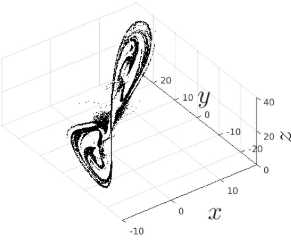
(a)

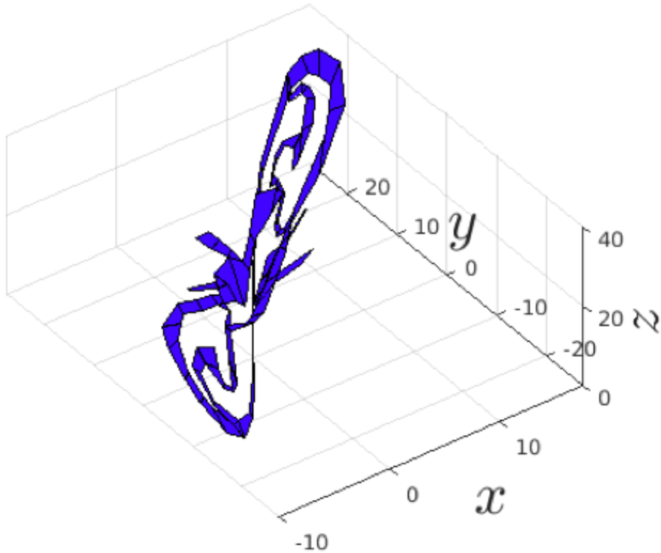
(b)

Figure 1: A snapshot of the LOrenz Random Attractor (LORA) Chekroun, Simonnet, and Ghil (2011), as shown by Charó et al. (2021) (2021). (a) The sieved three-dimensional point cloud; and (b) the BraMAH cell complex of dimension $d=2$ for this point cloud.

An example of a BraMAH cell complex $K(L)$ for the Lorenz attractorLorenz (1963) is provided in Figure 2(a). This cell complex is characterized by a key feature, namely the "sowing together" of the two wings of the butterfly by their interconnection through the two $1$-cells that are highlighted in color. This structural element assumes a pivotal role within the cell complex and the subsequent tracking of the flow supported on the complex.

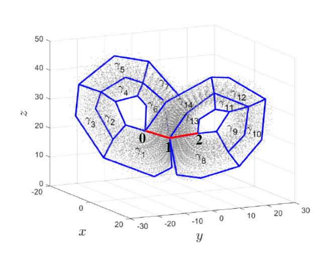
(a) $K(L)$

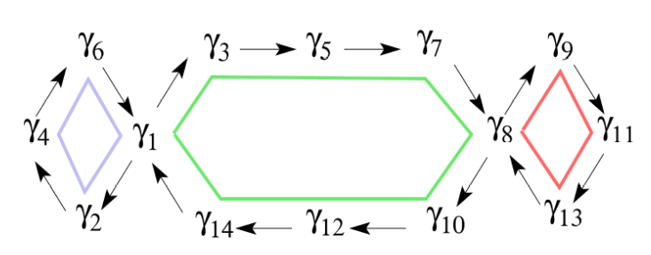
(b) $G(L)$

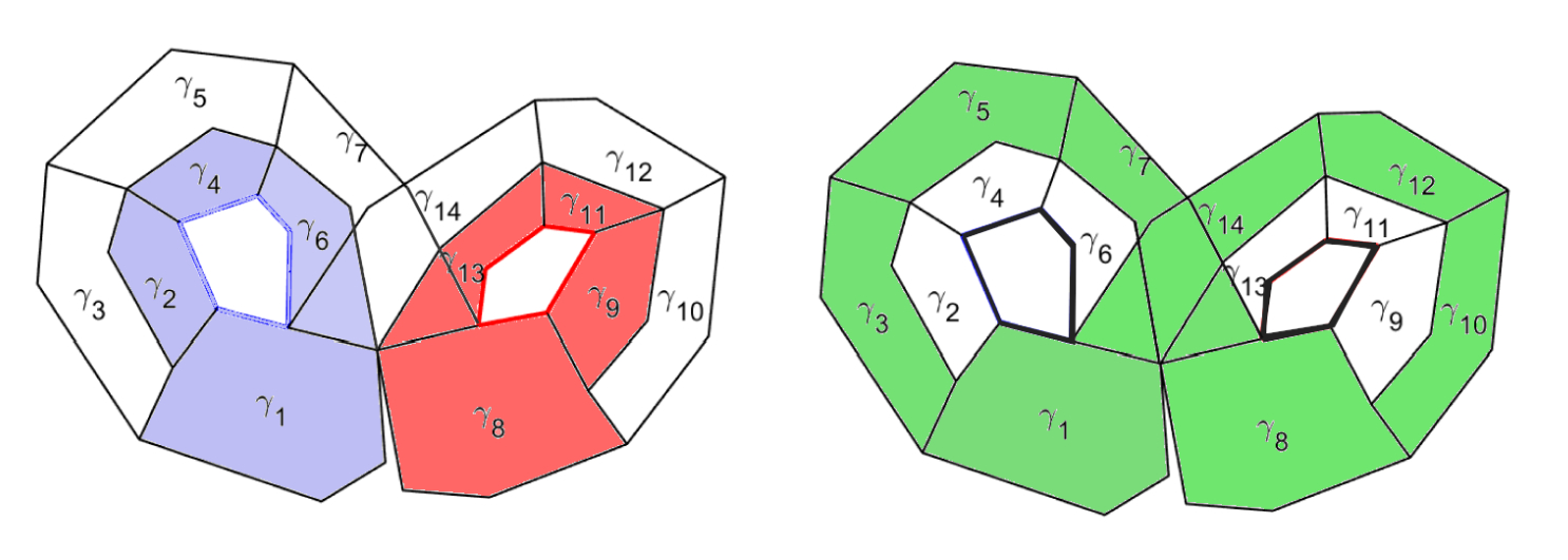
(c) generatexes

Figure 2: A templex $T(L)=(K(L),G(L))$ for a three-dimensional point cloud $L$ corresponding to the Lorenz attractor Lorenz (1963). (a) The BraMAH cell complex $K(L)$; the two $1$-cells colored in red constitute the joining line $J=\langle 0,1\rangle\cup\langle 1,2\rangle$. (b) The digraph $G(L)$ and its three cycles.(c) The three generatexes corresponding to the cycles in $G(L)$.

II.2 The joining locus and the digraph

In general, any BraMAH complex $K$ of dimension $d$ is said to have a joining locus if there are $(d-1)$-cells shared by at least three distinct $d$-cells. If $d=2$, the joining locus is called a joining line, as it is composed of $1$-cells. Joining lines can be seen as the analogs of the components of a Poincaré section. The Lorenz attractor is thus found to have a two-component joining locus, formed by the $1$-cells $\langle 0,1\rangle$ and $\langle 1,2\rangle$.

Let us now consider the underlying flow across the joining locus as depicted in Figure 2(b). The flow goes from the $2$-cells $\gamma_{6}$ and $\gamma_{7}$ into $\gamma_{1}$ through $\langle 0,1\rangle$, and it goes from $\gamma_{13}$ and $\gamma_{14}$ into $\gamma_{8}$ through $\langle 1,2\rangle$. We discriminate between these 2-cells according to the sense of the flow: $\gamma_{6}$, $\gamma_{7}$, $\gamma_{13}$ and $\gamma_{14}$ are the ingoing cells; and $\gamma_{1}$, $\gamma_{8}$ are the outgoing cells.

Defining flow paths on the cell complex is straightforward: it can be specified not only for the cells abutting the joining locus but also for the rest of the $2$-cells, leading to a digraph whose nodes coincide with the $2$-cells and whose edges determine whether the nodes are connected by the flow. As previously stated in Sect. I, we call the mathematical object formed by the cell complex $K$ and the associated digraph $G$ a templex.

Homologies provide the proof that nontrivial loops in the cell complex are fundamental for distinguishing different topological structures. Can we find nontrivial loops in the digraph that capture distinct essential properties of the flow along the structure? In fact, we can introduce a few definitions to capture such properties, just as we have retained the essential properties of the structure itself through the computation of the homology group generators.

A nontrivial loop in the digraph will be called a generatex. More precisely, a generatex is a subtemplex whose subgraph corresponds to a cycle in the digraph and the subcomplex is the set of cells corresponding to that cycle. As the number of cells in a cell complex is arbitrary, we define an equivalence relation to obtain a single representative for each group of equivalent generatexes, much like what is done with $k$-generators in homology group theory, leaving us with the minimal set of representative generatexes for a given point cloud.

Two generatexes are equivalent if they share the same set of ingoing and outgoing cells. A representative generatex is said to be of order $p$, with $p\in\mathbb{N}$ and $p\geq 1$, if the cycle has $p$ distinct ingoing nodes that correspond to the ingoing cells.

Last but not least, just as torsion groups can be computed alongside homology groups—enabling, for instance, the distinction between a simple strip and a Möbius strip — it is also possible to detect local twists in a templex by computing its stripexes. A stripex is associated with a representative generatex. For a simple generatex ($p=1$), the stripex coincides with the generatex and corresponds to the path from the outgoing cell to the ingoing cell. When the order of the generatex is greater than one ($p>1$), it can be decomposed into $p$ stripexes, each defined as the subset of the generatex corresponding to the path between an outgoing cell and an ingoing cell. A stripex is said to have a local twist if the free edges of the subcomplex associated with it change their relative positions.

Figure 2(b) shows the digraph $G(L)$. The generatex set is formed by three elements (see Fig. 2):

$$\mathcal{G}_{1}(L) =\{\gamma_{1}\rightarrow\gamma_{2}\rightarrow\gamma_{4}\rightarrow\gamma_{6}\rightarrow\gamma_{1}\},$$ (1a)

$$\mathcal{G}_{2}(L) =\{\gamma_{8}\rightarrow\gamma_{9}\rightarrow\gamma_{11}\rightarrow\gamma_{13}\rightarrow\gamma_{8}\},$$ (1b)

$$\mathcal{G}_{3}(L) =\{\gamma_{1}\rightarrow\gamma_{3}\rightarrow\gamma_{5}\rightarrow\gamma_{7}\rightarrow\gamma_{8}$$

$$\hskip 42.67912pt\rightarrow\gamma_{10}\rightarrow\gamma_{12}\rightarrow\gamma_{14}\rightarrow\gamma_{1}\}.$$ (1c)

The first two are of order 1, while the third one is of order 2 and can be separated into two stripexes. The stripex set has four elements, namely:

$$\mathcal{S}_{1}(L) =\{\gamma_{1}\rightarrow\gamma_{2}\rightarrow\gamma_{3}\},$$ (2a)

$$\mathcal{S}_{2}(L) =\{\gamma_{8}\rightarrow\gamma_{7}\rightarrow\gamma_{6}\},$$ (2b)

$$\mathcal{S}_{3}(L) =\{\gamma_{1}\rightarrow\gamma_{2}\rightarrow\gamma_{4}\},$$ (2c)

$$\mathcal{S}_{4}(L) =\{\gamma_{8}\rightarrow\gamma_{7}\rightarrow\gamma_{5}\}.$$ (2d)

Identifying a generatex or a stripex in the phase space is simple in the case of a templex, as the coordinates of the $0$-cells of the BraMAH complex are directly provided by the construction. Stripexes $\mathcal{S}_{2}(L)$ and $\mathcal{S}_{4}(L)$ have a twist. The free edges for $\mathcal{S}_{2}$ are $\langle 1,4,9,2\rangle$ and $\langle 0,3,7,8,1\rangle$; and for $\mathcal{S}_{4}$ they are $\langle 2,6,12,11,1\rangle$ and $\langle 1,5,10,0\rangle$.

Armed with this set of concepts, we can describe in detail not only the structure associated with a deterministic attractor in phase space but also the representative flow paths around the structure, provided it has a joining locus, without which alternative paths — and, therefore, chaos — would not be possible. In the case of a random attractor, its phase space involves a flow linking different snapshots, each of which is approximated by a complex of dimension $2$. It follows that a digraph can be constructed to track the way in which $1$-holes evolve, describing the different "moments in the life" of the attractor Charó, Ghil, and Sciamarella (2023). However, this stochastic flow should not be confused with the flow of a deterministic attractor, which occurs between the cells of a single cell complex.

III A low-order model of the wind-driven circulation and its templex

Following Pierini 2011 and Pierini, Ghil, and Chekroun2016, we investigate here a 4-D spectral QG model of the wind-driven, double-gyre ocean circulation in midlatitudes. The full model’s streamfunction is expanded in a rectangular domain according to

$$\psi(x,y,t)=\sum_{i=1}^{4}\Psi_{i}(t)\lvert i\rangle.$$ (3)

The orthonormal basis $\lvert i\rangle$ is defined by:

$$\lvert 1\rangle=e^{-\alpha x}\sin x\sin y,$$ (4a)

$$\lvert 2\rangle=e^{-\alpha x}\sin x\sin 2y,$$ (4b)

$$\lvert 3\rangle=e^{-\alpha x}\sin 2x\sin y,$$ (4c)

$$\lvert 4\rangle=e^{-\alpha x}\sin 2x\sin 2y,$$ (4d)

with a constant value for $\alpha>0$. This basis satisfies the free-slip boundary conditions along the boundaries of the rectangular domain and it also accounts for the oceanic flow’s western boundary layer, often referred to in physical oceanography as westward intensification Gill (1982).

The set of four nonlinear coupled ordinary differential equations governing the evolution of the state vector $\mathbf{\Psi}(t)=(\Psi_{1}(t),\Psi_{2}(t),\Psi_{3}(t),\Psi_{4}(t))^{\rm T}$ can be expressed in vector-matrix notation as:

$$\frac{d\mathbf{\Psi}}{dt}+\mathbf{\Psi}\mathbf{J}\mathbf{\Psi}+\mathbf{L}\mathbf{\Psi}=\Gamma(t)\mathbf{w},$$ (5a)

$$\Gamma(t)=\gamma[1+\epsilon sin(\omega t)],$$ (5b)

where $\epsilon$ and $\gamma$ are real dimensionless constants.

In the forcing term on the right-hand side of Eq. (5a), $\mathbf{w}$ gives the spatial structure of the wind stress curl and $\Gamma(t)$ defines the time dependence of its intensity; see Pierini 2011 for the definition of $\mathbf{J}$, $\mathbf{L}$ and $\mathbf{w}$. In the autonomous case of $\epsilon=0$, the forcing term is a constant, $\Gamma(t)=\gamma$, and self-sustained ROs occur for $\gamma>1$. These equations are integrated numerically using the Bulirsch–Stoer method Press (1992). Each integration is carried out for a duration that (a) sufficiently exceeds the spin-up time in a given scenario; and (b) lasts for long enough thereafter to permit observing the attractor and characterizing it.

If the forcing corresponds to a periodic function, as is the case in this study, a snapshot attractor exists and can be approximated simply by forward integration.

III.1 Templex analysis for the autonomous case

In this section, we examine the autonomous case of $\epsilon=0$, where the forcing $\Gamma(t)=\gamma$ is a constant and the phase space is spanned by $(\Psi_{1},\Psi_{2},\Psi_{3},\Psi_{4})^{\rm T}$, cf. Eqs. (3)–(5). Templex analysis will be conducted to elucidate the intrinsic variability of the strange attractor that emerges when the parameter value is $\gamma=1.35$. The bifurcation diagram for the autonomous case is shown in Fig. 1 of Pierini, Chekroun, and Ghil (2018) and at this value of $\gamma$, large-amplitude ROs characterize the model’s autonomous behavior. One such RO is shown in Fig. 3.

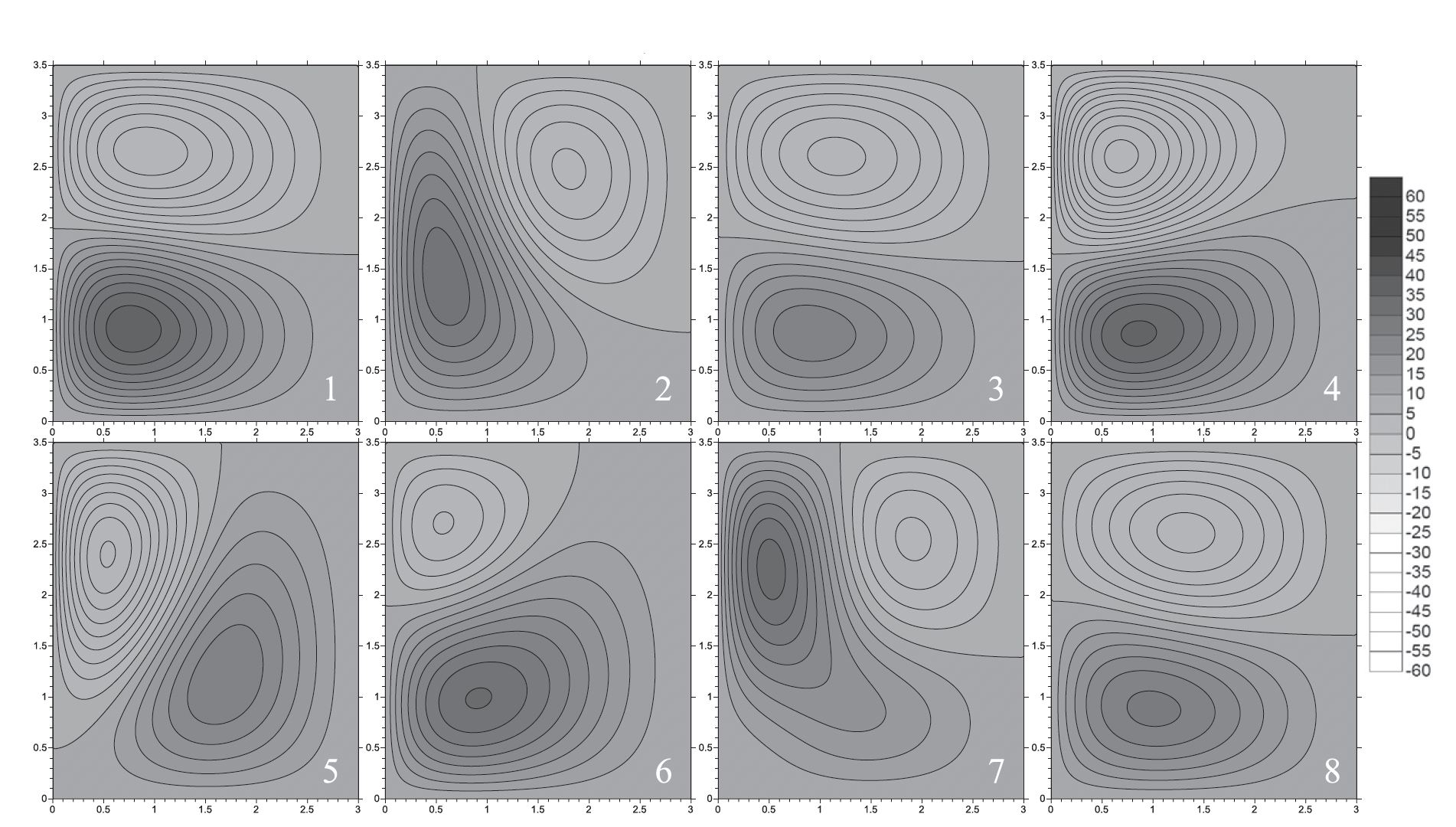
Figure 3: Streamfunction evolution for a relaxation oscillation (RO) of the idealized ocean model in the autonomous case, with $\gamma=1.043$. The order of the panels is indicated by the white numerals in the lower-right corner of the panels. Taken from Ref. Pierini (2011)

The BraMAH cell complex $K_{1}$ that approximates the point cloud in four dimensions is shown in Figure 4(a) projected onto the subspace $(\Psi_{1},\Psi_{3},\Psi_{4})$. To improve clarity, the cell complex $K_{1}$ was simplified by merging some of the 2-cells in $\bar{K}_{1}$, as shown in Figure 4(b), where the heavy pink line segment indicates the joining locus $\langle 0,1\rangle$. This simplification did not alter the topological structure of the original complex.

Note that the 1-cell $\langle 18,19,20\rangle$ is a splitting locus, where the $0$-cell $\langle 19\rangle$ is a tearing point and is called a splitting 0-cell. The flow that emanates from $\sigma_{12}$ bifurcates into two branches, $\sigma_{1}$ and $\sigma_{2}$, due to the splitting 0-cell. We name the templex of this case $T_{1}=(\bar{K}_{1},G_{1})$.

The digraph $G_{1}$ is shown in Figure 5. Here the ingoing and outgoing cells are represented by squares and circles, respectively; and the cycles in $G_{1}$ are colored. These two cycles (red and blue ) correspond to the two simple generatexes $\mathcal{G}_{1}$ and $\mathcal{G}_{2}$:

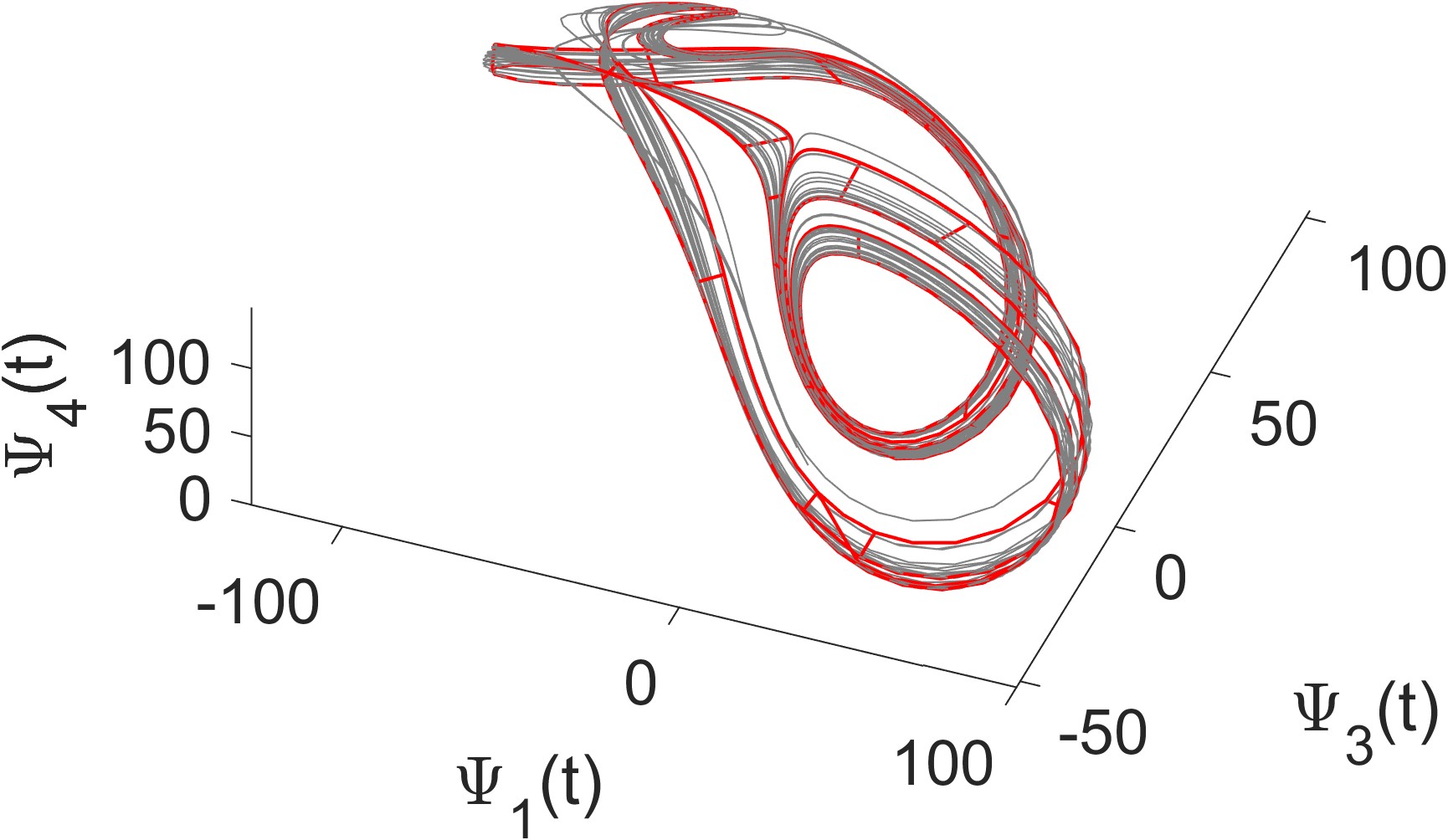
(a) Point cloud and complex $K_{1}$

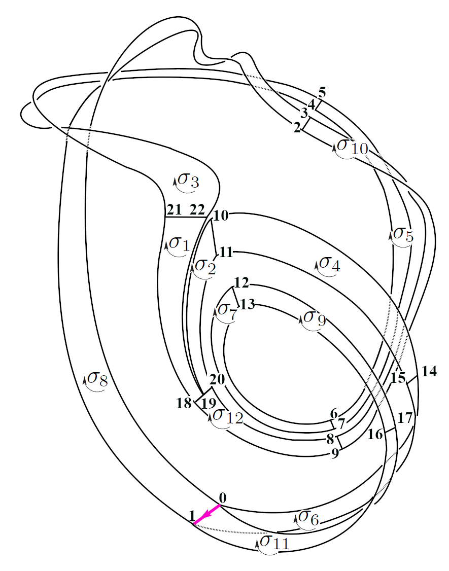
(b) Simplified complex $\bar{K}_{1}$

Figure 4: Topological analysis of the autonomous model version in the RO domain, for $\gamma=1.35$. (a) Point cloud (gray dots) juxtaposed with the BraMAH cell complex $K_{1}$ (in red) for a projection onto the $(\psi_{1},\psi_{3},\psi_{4})$-subspace; and (b) diagram of the simplified cell complex $\bar{K}_{1}$. The oriented heavy pink line indicates the joining 1-cell $\langle 0,1\rangle$.

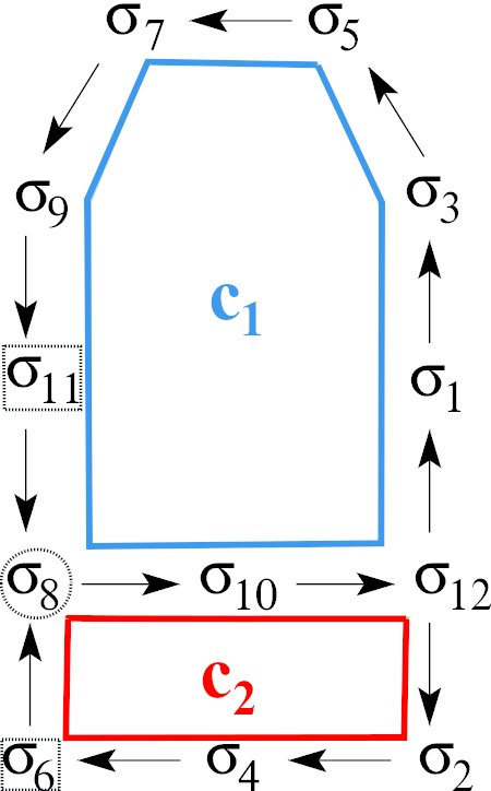
Figure 5: Digraph $G_{1}$ here corresponds to the templex $T_{1}=(\bar{K}_{1},G_{1})$ for the autonomous case in Fig. 4; ingoing and outgoing cells are squared and circled, respectively. The cycles $c_{1}$ and $c_{2}$ in $G_{1}$ are marked in red and blue, and they correspond to the two generatexes $\mathcal{G}_{1}$ and $\mathcal{G}_{2}$, respectively.

$$\mathcal{G}_{1}(T_{1}) =\{\sigma_{8}\rightarrow\sigma_{10}\rightarrow\sigma_{12}\rightarrow\sigma_{2}\rightarrow\sigma_{4}$$

$$\qquad\rightarrow\sigma_{6}\rightarrow\sigma_{8}\},$$ (6a)

$$\mathcal{G}_{2}(T_{1}) =\{\sigma_{8}\rightarrow\sigma_{10}\rightarrow\sigma_{12}\rightarrow\sigma_{1}\rightarrow\sigma_{3}\rightarrow\sigma_{5}\rightarrow\sigma_{7}$$

$$\qquad\rightarrow\sigma_{9}\rightarrow\sigma_{11}\rightarrow\sigma_{8}\}.$$ (6b)

These two generatexes are plotted in Fig. 6.

(a) $\mathcal{G}_{1}(T_{1})$

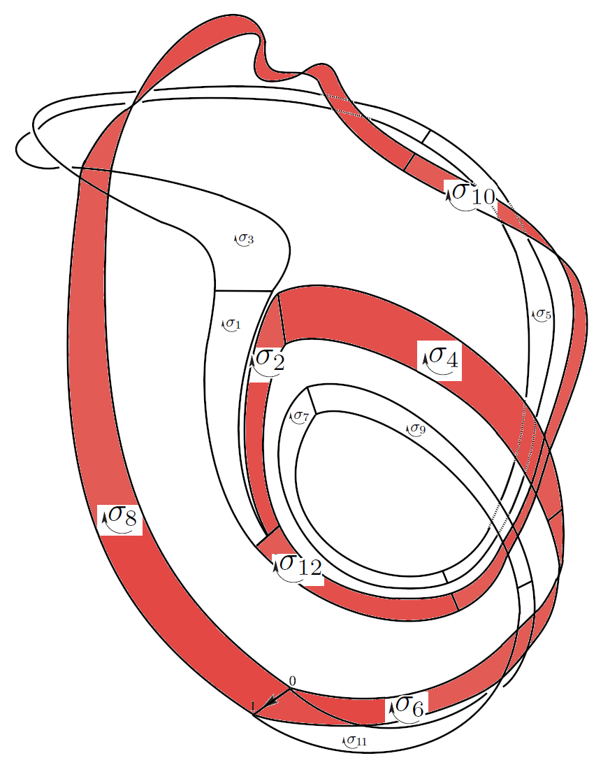
(b) $\mathcal{G}_{2}(T_{1})$

Figure 6: The two generatexes of the autonomous case in Fig. 4, shown in the simplified cell complex $\bar{K}_{1}$: (a) $\mathcal{G}_{1}(T_{1})$; and (b) $\mathcal{G}_{2}(T_{1})$.

The stripex set has two elements, namely,

$$\mathcal{S}_{1}(T_{1}) =\{\sigma_{8}\rightarrow\sigma_{10}\rightarrow\sigma_{12}\rightarrow\sigma_{2}\rightarrow\sigma_{4}\rightarrow\sigma_{6}\},$$ (7a)

$$\mathcal{S}_{2}(T_{1}) =\{\sigma_{8}\rightarrow\sigma_{10}\rightarrow\sigma_{12}\rightarrow\sigma_{1}\rightarrow\sigma_{3}\rightarrow\sigma_{5}\rightarrow$$

$$\hskip 42.67912pt\sigma_{7}\rightarrow\sigma_{9}\rightarrow\sigma_{11}\}.$$ (7b)

Stripex $\mathcal{S}_{1}(T_{1})$ has a twist, and its free edges are:

$$\langle 1,3,8,20,19,22,5,7,12,17,0\rangle,\quad\mbox{and}$$

$$\langle 0,2,9,18,21,4,6,13,16,1\rangle.$$ (8)

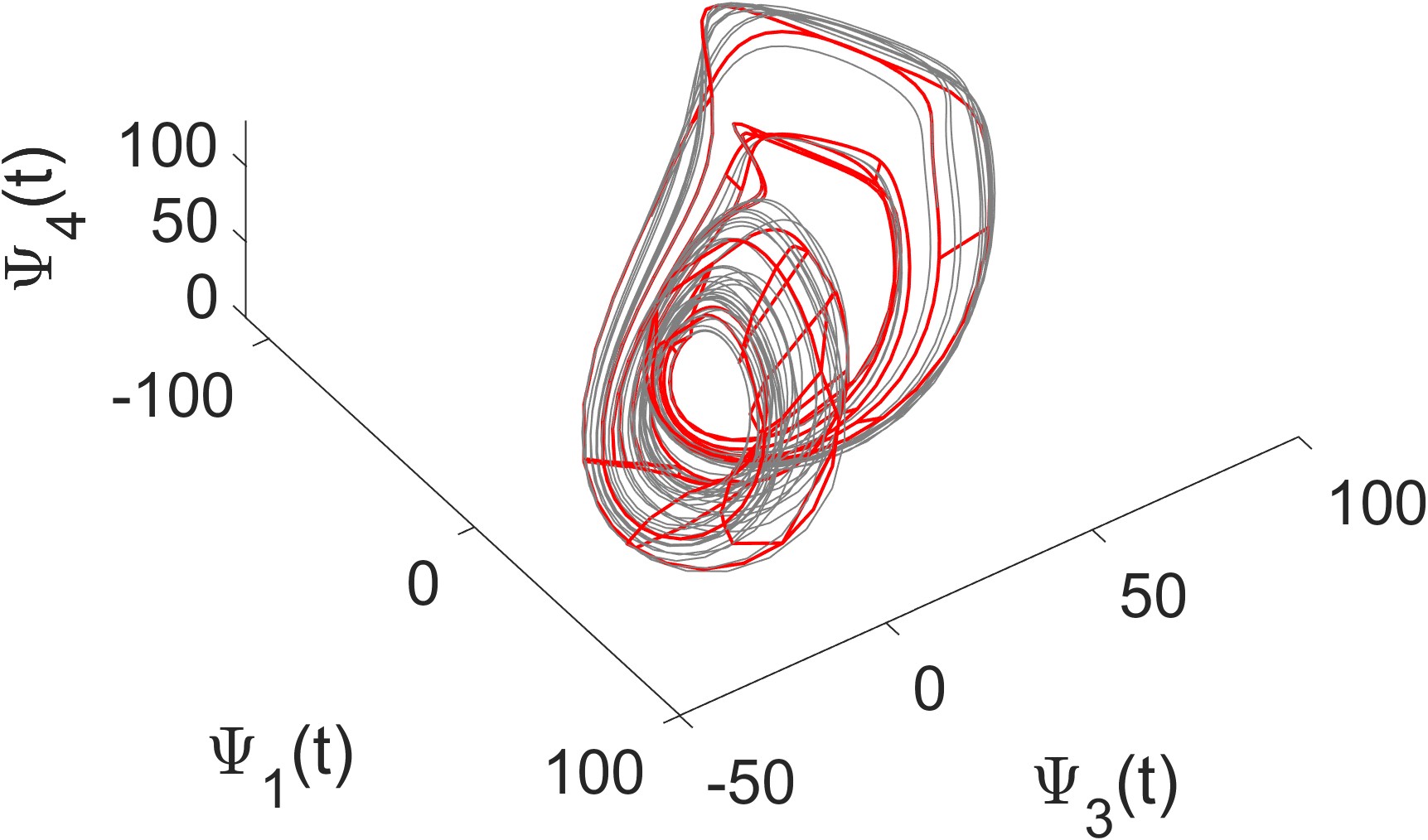
(a) Point cloud and complex $K_{2}$

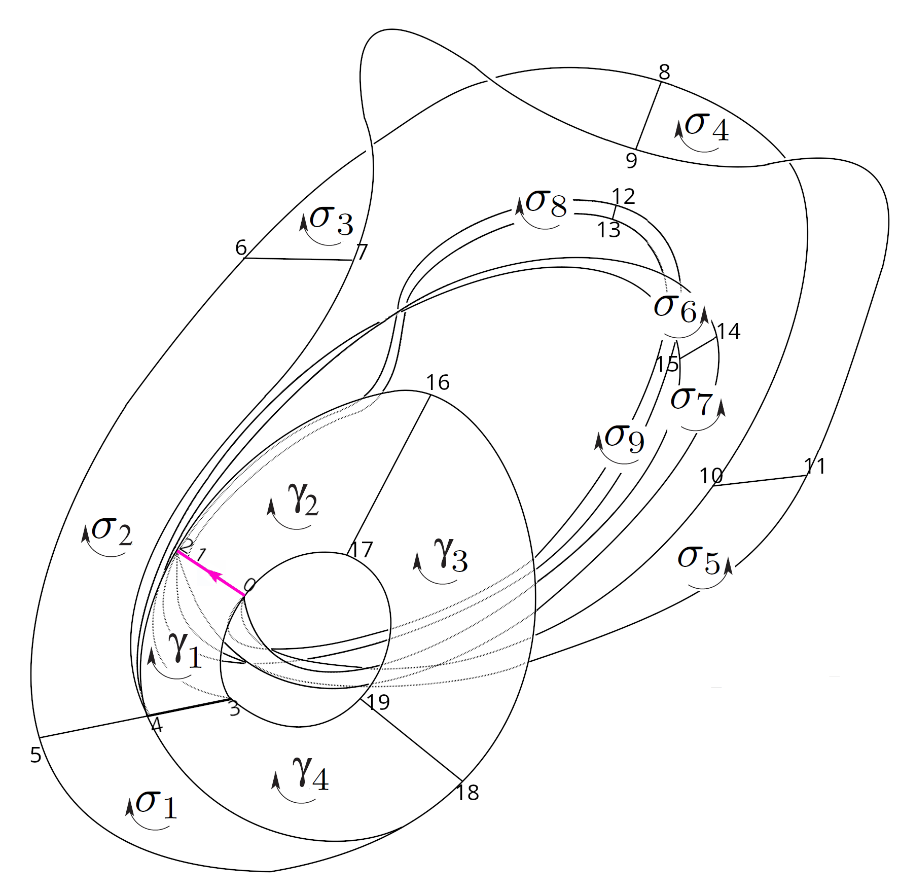
(b) Simplified complex $\bar{K}_{2}$

Figure 7: Topological analysis of the nonautonomous model version for $\gamma=1.10$ and $\epsilon=0.20$. (a) Plot of the point cloud (gray dots) juxtaposed with the BraMAH cell complex (in red) in a $(\psi_{1},\psi_{3},\psi_{4})$ projection. (b) Diagram of the simplified cell complex $\bar{K}_{2}$, where $\gamma_{i}$ ($i=1,\ldots,4$) are 3-cells and $\sigma_{j}$ ($j=1,\ldots,9$) are 2-cells. The heavy pink line segments indicate the joining locus at $\langle 0,1,2\rangle$ and the splitting locus at $\langle 4,3\rangle$.

III.2 Templex analysis for a nonautonomous case

In this section, we analyze the periodically forced case in the phase space spanned by $(\Psi_{1},\Psi_{2},\Psi_{3},\Psi_{4})^{\rm T}$, cf. Eqs. (3)–(5); the parameter values are $\gamma=1.10$ and $\epsilon=0.20$, and the forcing period is $\bar{T}_{p}=2\pi/\omega=30$ yr. The cell complex $K_{2}$ and its simplified form $\bar{K}_{2}$ are shown in Figure 7; the projection in panel (a) here is onto the same subspace $(\Psi_{1},\Psi_{3},\Psi_{4})$ as in Figure 4(a).

Notice that the presence of a time-dependent forcing transforms some of the 2-cells of the autonomous complex ($\sigma_{1},\sigma_{2},\sigma_{4},\sigma_{6},\sigma_{7},\sigma_{9}$, $\sigma_{11}$) into the 3-cells ($\gamma_{1}$,$\gamma_{2}$,$\gamma_{3}$,$\gamma_{4}$) of the nonautonomous case. Note that including a time-dependent forcing element into an autonomous system gives rise to a three-dimensional filled torus in the templex defined by the chain of 3-cells $\gamma_{1}$,$\gamma_{2}$,$\gamma_{3}$, and $\gamma_{4}$. This phenomenon has also been noticed in analyzing the templex properties of an idealized model of the Atlantic Meridional Overturning Circulation system Mosto et al. (2025).

Notice that there are two heavy lines in $\bar{K}_{2}$: the joining locus $\langle 0,1,2\rangle$ and the splitting locus $\langle 4,3\rangle$. At the splitting locus, the trajectories can take two distinct paths: one leading from $\gamma_{4}$ to $\gamma_{1}$, and the other from $\gamma_{4}$ to $\sigma_{6}$. This splitting does not contradict the uniqueness of solutions, as the locus encompasses cells of different dimensions. In the digraph $G_{2}$ of Figure 8, the ingoing and outgoing cells are represented by squares and circles, respectively. Together, the cell complex $\bar{K}_{2}$ and its corresponding digraph $G_{2}$ in Figure 8 form the templex $T_{2}=(\bar{K}_{2},G_{2})$. The filled torus leads to the emergence of multiple branches that are encountered at the joining locus $\langle 0,1,2\rangle$, introducing two additional generatexes compared to the autonomous case.

Figure 8: Digraph $G_{2}$ corresponding to the templex $T_{2}=(\bar{K}_{2},G_{2})$ for the nonautonomous case in Fig. 7; ingoing and outgoing cells are embedded in squares and circles, respectively. The cycles $c_{1},c_{2},c_{3},c_{4}$ in $G_{2}$ are marked by distinct colors and they correspond to the four generatexes $\mathcal{G}_{1},\mathcal{G}_{2},\mathcal{G}_{3},\mathcal{G}_{4}$, respectively.

The generatex set in Figure 9 is formed by four elements:

$$\mathcal{G}_{1}(T_{2}) =\{\gamma_{2}\rightarrow\gamma_{3}\rightarrow\gamma_{4}\rightarrow\gamma_{1}\rightarrow\gamma_{2}\},$$ (9a)

$$\mathcal{G}_{2}(T_{2}) =\{\gamma_{2}\rightarrow\gamma_{3}\rightarrow\gamma_{4}\rightarrow\sigma_{6}\rightarrow\sigma_{7}\rightarrow\gamma_{2}\},$$ (9b)

$$\mathcal{G}_{3}(T_{2}) =\{\gamma_{2}\rightarrow\gamma_{3}\rightarrow\gamma_{4}\rightarrow\sigma_{1}\rightarrow\sigma_{2}\rightarrow\sigma_{3}$$

$$\hskip 42.67912pt\rightarrow\sigma_{4}\rightarrow\sigma_{5}\rightarrow\gamma_{2}\},$$ (9c)

$$\mathcal{G}_{4}(T_{2}) =\{\gamma_{2}\rightarrow\gamma_{3}\rightarrow\gamma_{4}\rightarrow\gamma_{1}\rightarrow\sigma_{8}\rightarrow\sigma_{9}\rightarrow\gamma_{2}\}.$$ (9d)

Notice that all generatexes are stripexes since they are of order 1. In the case of generatex $\mathcal{G}_{4}(T_{2})$, two ingoing cells are involved in the cycle, $\gamma_{1}$ and $\sigma_{9}$. However, in this particular instance, the cycle includes the outgoing cell, denoted by $\gamma_{2}$ and continues through the cells labeled $\gamma_{3}$, $\gamma_{4}$ and $\gamma_{1}$. Notably, it does not return to $\gamma_{2}$: instead, it traverses the branch $\sigma_{8}$ and subsequently passes through $\sigma_{9}$, thus completing the cycle in $\gamma_{2}$. Consequently, the ingoing cell in this generatex is $\sigma_{9}$.

The outcome is the set of four stripexes, namely,

$$\mathcal{S}_{1}(T_{2}) =\{\gamma_{2}\rightarrow\gamma_{3}\rightarrow\gamma_{4}\rightarrow\gamma_{1}\},$$ (10a)

$$\mathcal{S}_{2}(T_{2}) =\{\gamma_{2}\rightarrow\gamma_{3}\rightarrow\gamma_{4}\rightarrow\gamma_{1}\rightarrow\sigma_{6}\rightarrow\sigma_{7}\},$$ (10b)

$$\mathcal{S}_{3}(T_{2}) =\{\gamma_{2}\rightarrow\gamma_{3}\rightarrow\gamma_{4}\rightarrow\sigma_{1}\rightarrow\sigma_{2}\rightarrow\sigma_{3}\rightarrow\sigma_{4}\rightarrow\sigma_{5}\},$$ (10c)

$$\mathcal{S}_{4}(T_{2}) =\{\gamma_{2}\rightarrow\gamma_{3}\rightarrow\gamma_{4}\rightarrow\gamma_{1}\rightarrow\sigma_{8}\rightarrow\sigma_{9}\}.$$ (10d)

Stripexes $\mathcal{S}_{2}(T_{2})$ and $\mathcal{S}_{3}(T_{2})$ have a twist. The free edges for $\mathcal{S}_{2}$ are $\langle 2,16,18,20,4,15,0\rangle$ and $\langle 0,17,19,3,14,2\rangle$; while for $\mathcal{S}_{3}$ they are $\langle 2,16,18,20,5,6,8,10,0\rangle$ and $\langle 0,17,19,3,4,7,9,11,2\rangle$.

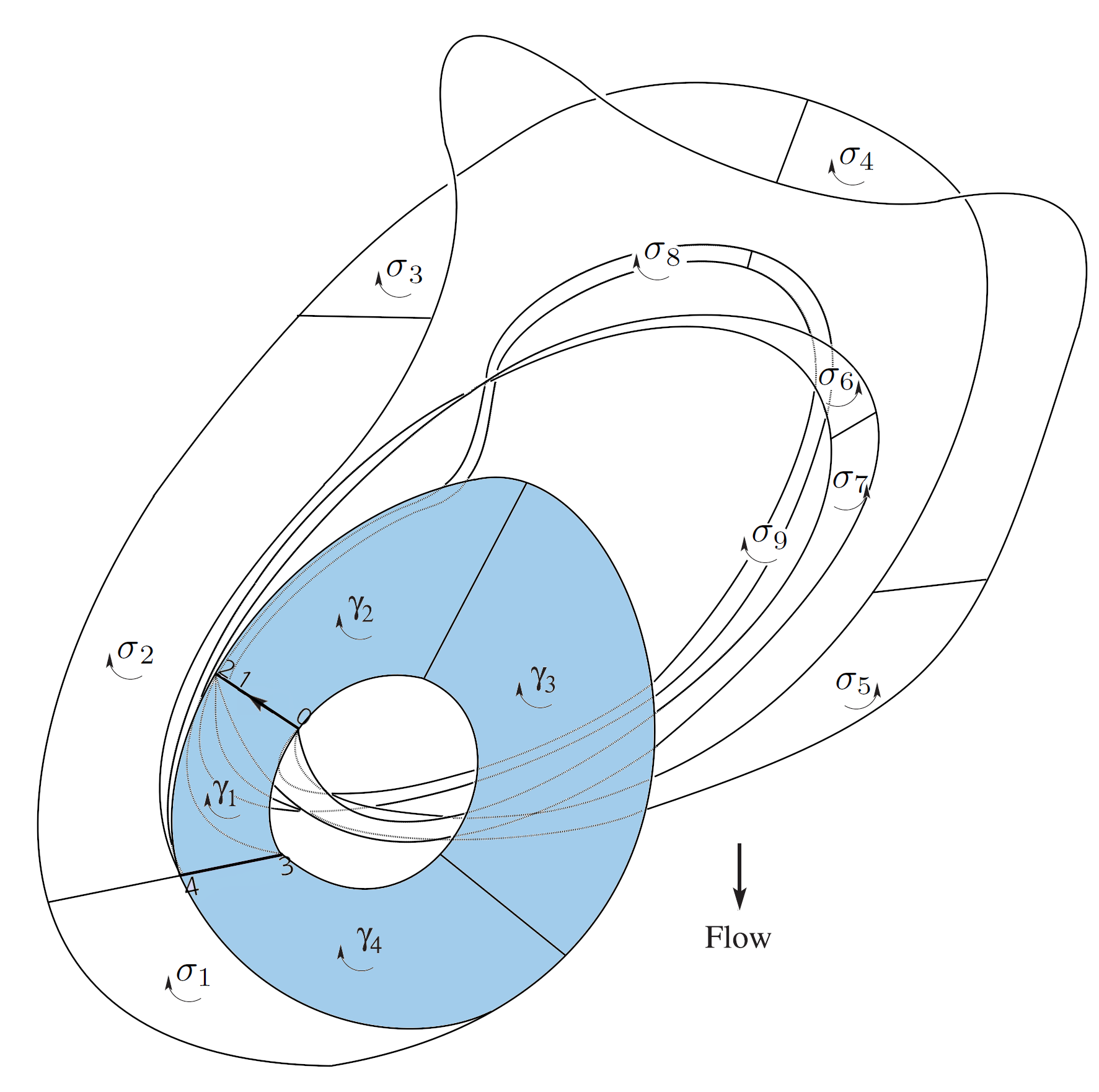
$\mathcal{G}_{1}(T_{2})$

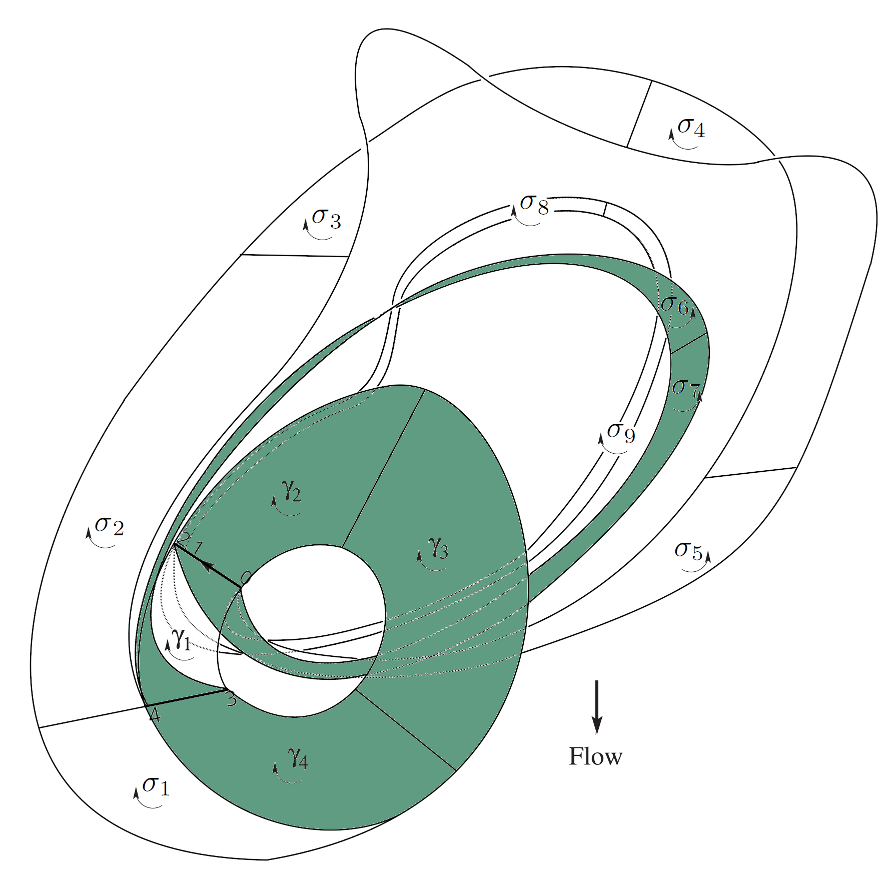
$\mathcal{G}_{2}(T_{2})$

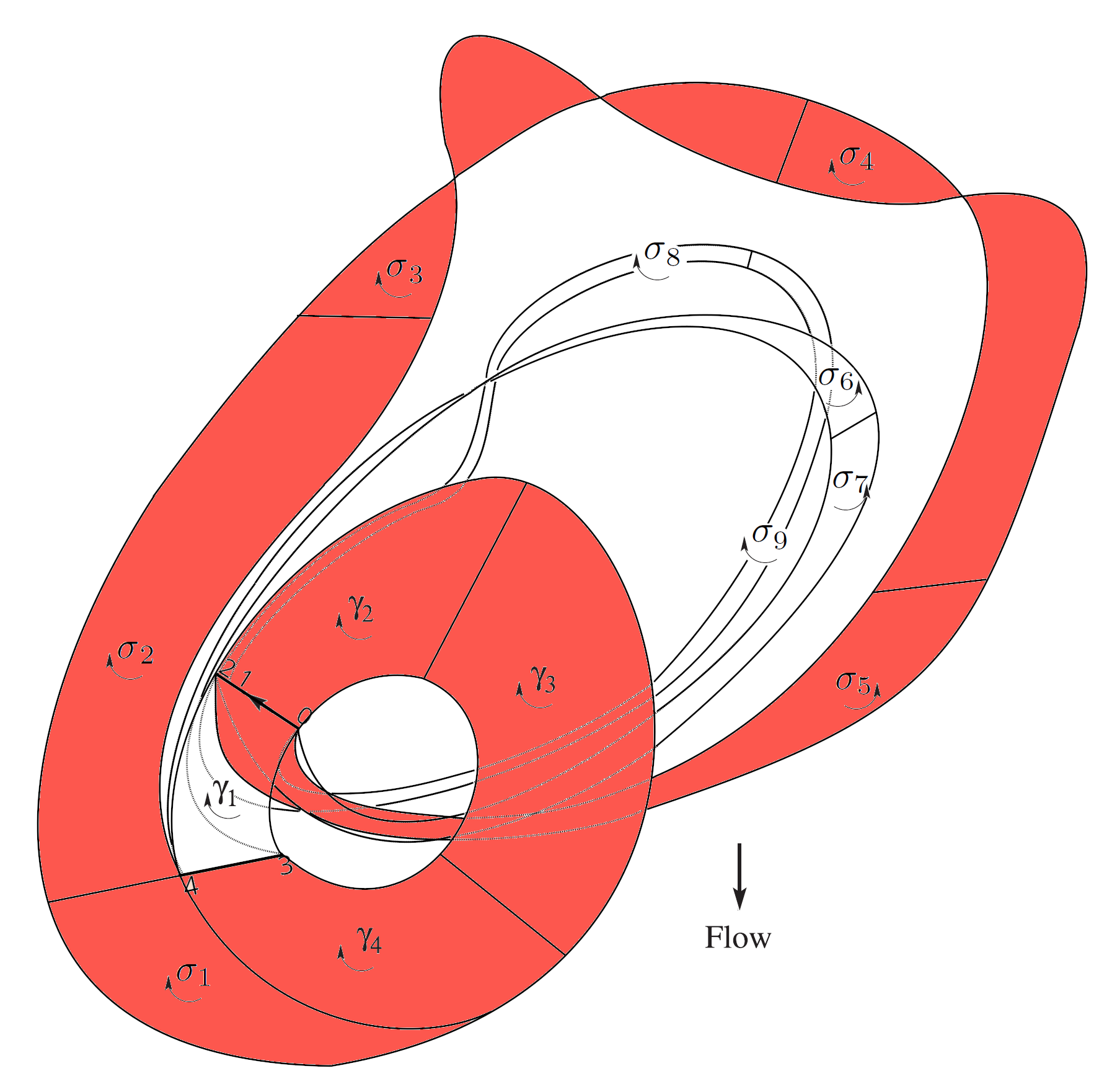
$\mathcal{G}_{3}(T_{2})$

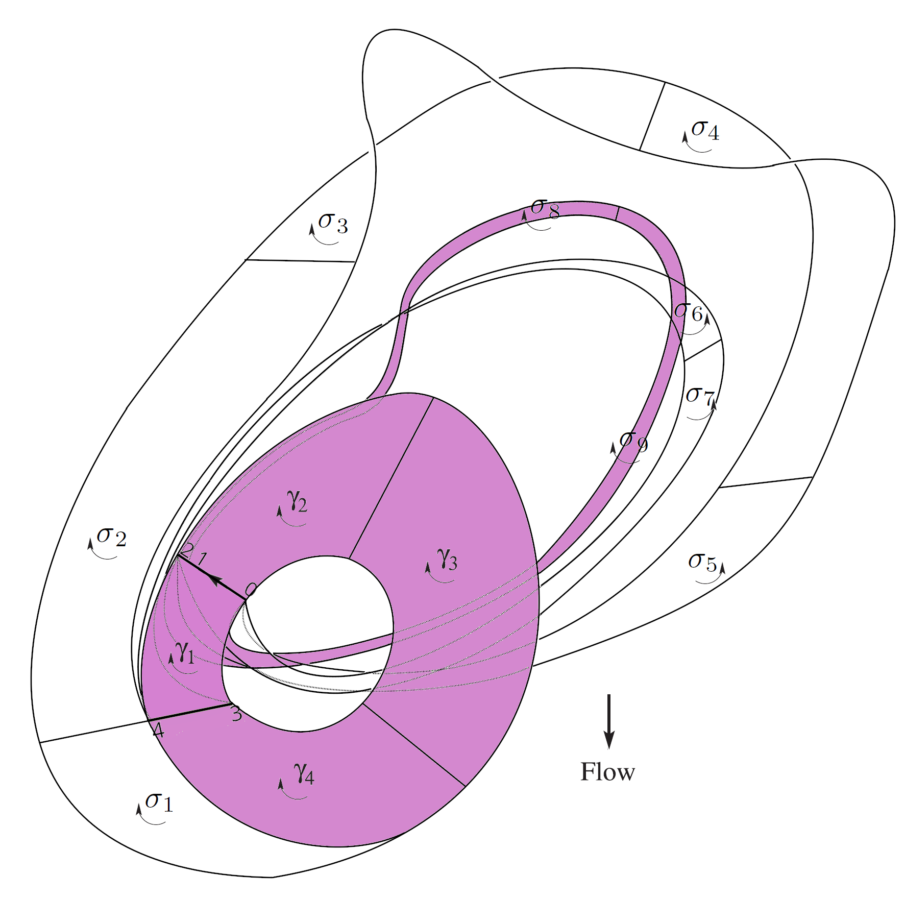
$\mathcal{G}_{4}(T_{2})$

Figure 9: Time series $\Psi_{1}(t)$ of an individual solution within the snapshot attractor, and the four generatexes $\mathcal{G}_{1},\mathcal{G}_{2},\mathcal{G}_{3},$ and $\mathcal{G}_{4}$ in the nonautonomous-case templex $T_{2}$, as seen within the cell complex $\bar{K}_{2}$. Segments of the time series $\Psi_{1}(t)$ are colored in accordance with the generatex through which the solution passes.

IV Snapshot attractor and templex

Figure 10: Evolution of the snapshot attractor over a time interval of length $T_{p}$.

As already mentioned in the Introduction, NDS theory differs from the much older and better known theory of autonomous attractors in an essential way. Classical theory applies to systems in which the forcing and coefficients are constant in time, and in which solutions exist for all time, from $t\to-\infty$ to $t\to+\infty.$ In NDS theory, the coefficients or forcing or both may depend on time, and solutions do not just depend on $t-t_{0},$ where $t_{0}$ is the initial time, but on both the initial time $s\equiv t_{0}$ and $t,$ the running time.

Accordingly, there are two kinds of attractors that can be defined for NDSs: pullback attractors (PBAs), obtained by letting $s\to-\infty$ for $t$ fixed Crauel and Flandoli (1994); Arnold (1988); Ghil, Chekroun, and Simonnet (2008), and forward attractors(FWAs), obtained by finding a special solution that does exist all the way to $+\infty$ and such that all solutions converge to it. Much more, in terms of conditions for existence and uniqueness, is known for PBAs than for the FWAs of NDSs Caraballo and Han (2017); Kloeden and Yang (2020). The latter have been called in the physical literature snapshot attractors by Namenson, Ott, and Antonsen (1996) and applied in the climate sciences by Drótos, Bódai, and Tél (2015) under this name.

Calculating a PBA does not require pulling back all the way to $-\infty$, only to a distance in time that equals a finite multiple of dissipation times, which depends on the precision with which we want to calculate the attractor, and is actually rather small Chekroun, Simonnet, and Ghil (2011); Charó et al. (2021). Still, it is more straightforward computationally to calculate an FWA or snapshot attractor, when one exists, even when it may not be unique Pierini, Ghil, and Chekroun (2016), and hence we do so here.

A snapshot attractor at time $t=T$ is the result of integrating a substantial array of initial conditions that coalesce, at least to within a good enough approximation, at the time $T$. To obtain the snapshot attractor of system (5) at time $T,$ an ensemble of $1.5\times 10^{5}$ random initial conditions lying in a hypercube $D\subset\mathbb{R}^{4}$ was integrated until the time $t=T$. In order to establish a basis for comparison between the templex approach and the snapshot approach in the nonautonomous case, the parameter values of the time-dependent forcing $\Gamma(t)$ were set to the values previously studied in Section III.2, namely $\gamma=1.10$ and $\epsilon=0.20$.

The temporal evolution of the snapshot attractor was investigated over a 400-year time interval. The transition time for satisfactory convergence to the attractor was of 66 yrs, after which the attractor became periodic, with a period of $T_{p}=30.09$ yr. In Figure 10, we show the snapshot attractor evolving over a full period $T_{p}$. Note the very small sampling deviation between the exact forcing period of $\bar{T}_{p}=30.00$ yr and the periodicity of the rather well converged snapshot attractor $T_{p}=30.09$ yr.

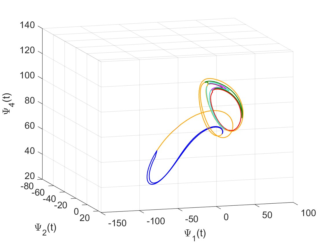
$t=0~T_{p}$

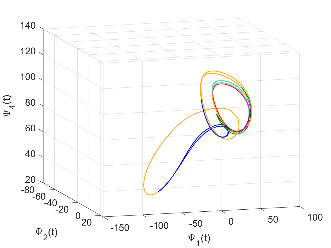
$t=0.05~T_{p}$

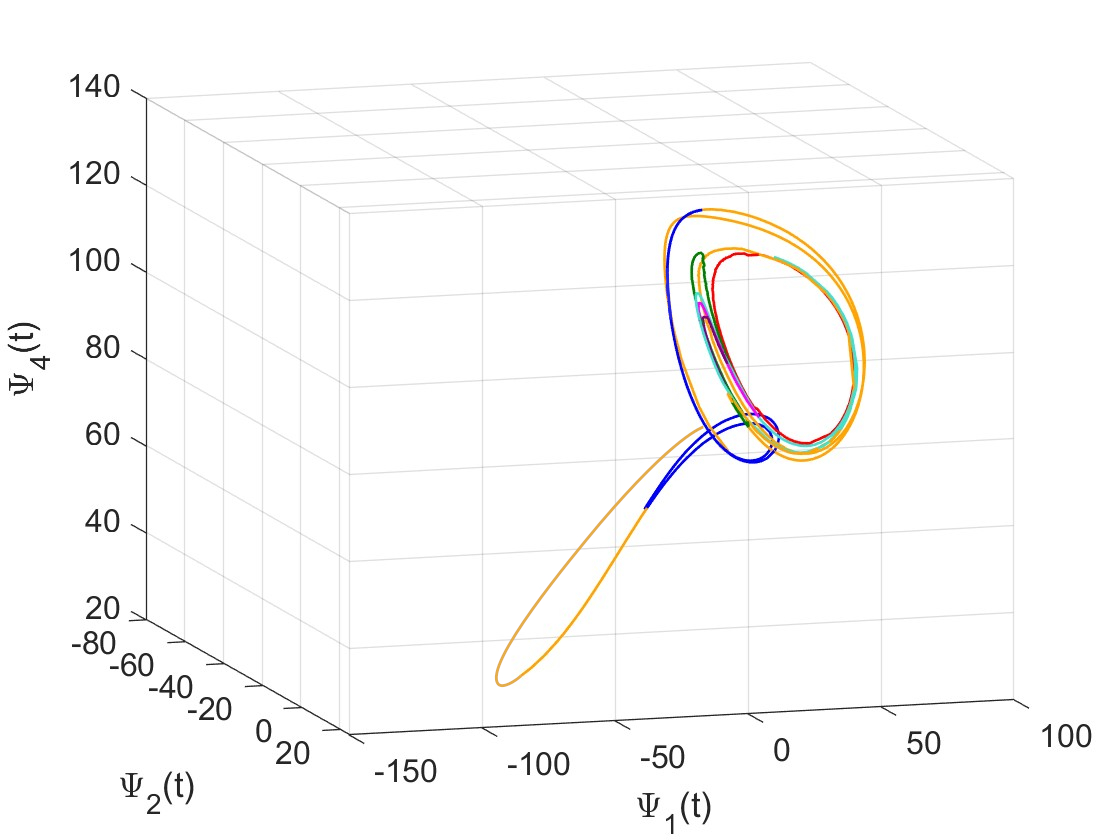
$t=0.1~T_{p}$

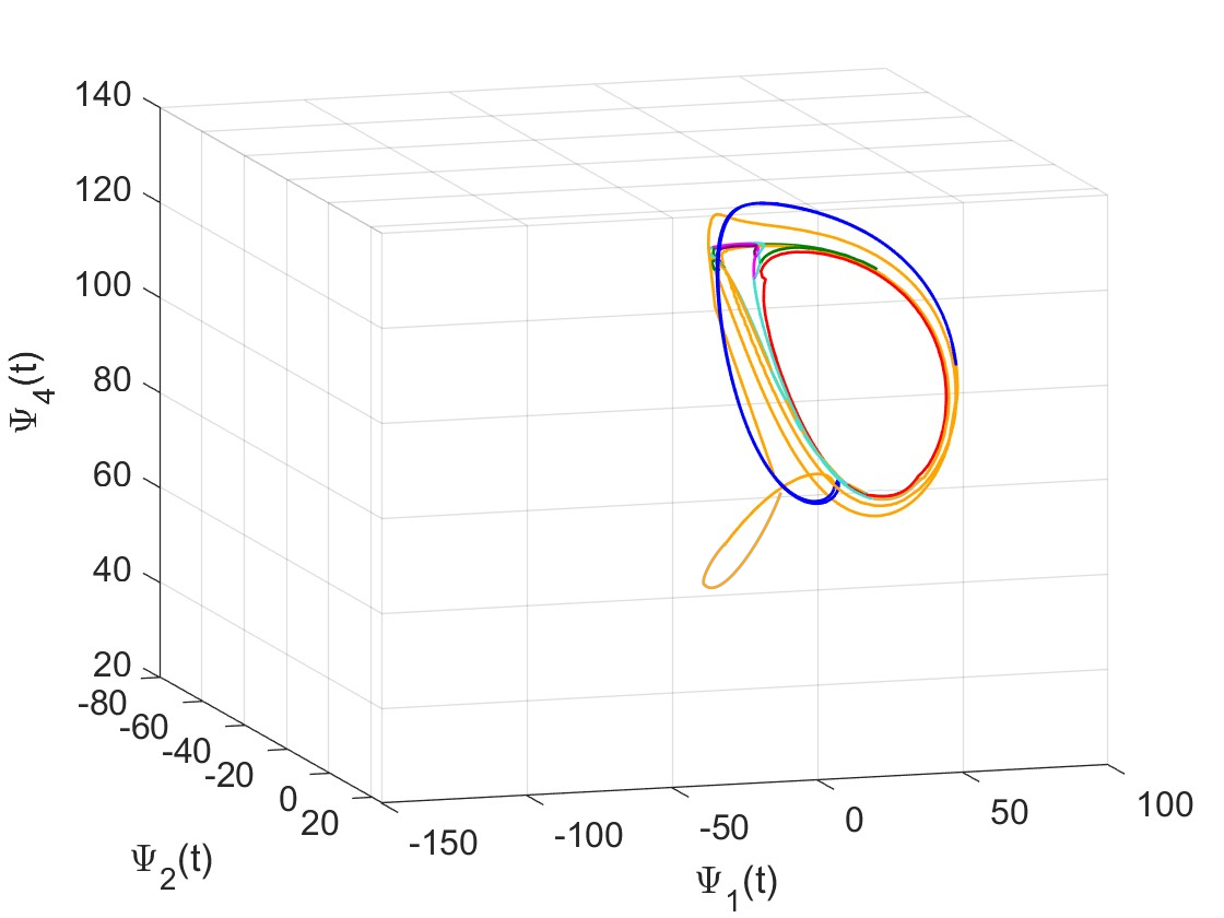
$t=0.15~T_{p}$

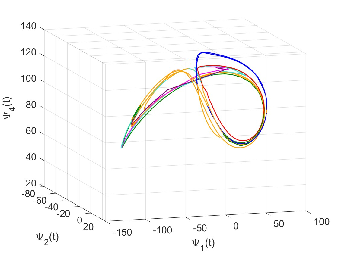
$t=0.2~T_{p}$

Figure 11: Homological description of five successive snapshots at $t=0,0.05~T_{p},0.10~T_{p},0.15~T_{p},0.20~T_{p}$), with seven 1-holes shown in different colors. The snapshots are shown projected onto the $(\Psi_{1},\Psi_{2},\Psi_{4})$-subspace.

The initial five snapshots depicted in Figure 10 are presented in Fig. 11 via a homological description in terms of seven 1-holes. In the figure, these holes undergo a continuous stretching and squeezing process.

V Topological Variability Modes

(a) $\mathcal{G}_{1}$, $\tau_{1}=[94.58,95.88]$ yrs, $|\tau_{1}|=1.30$ yrs.

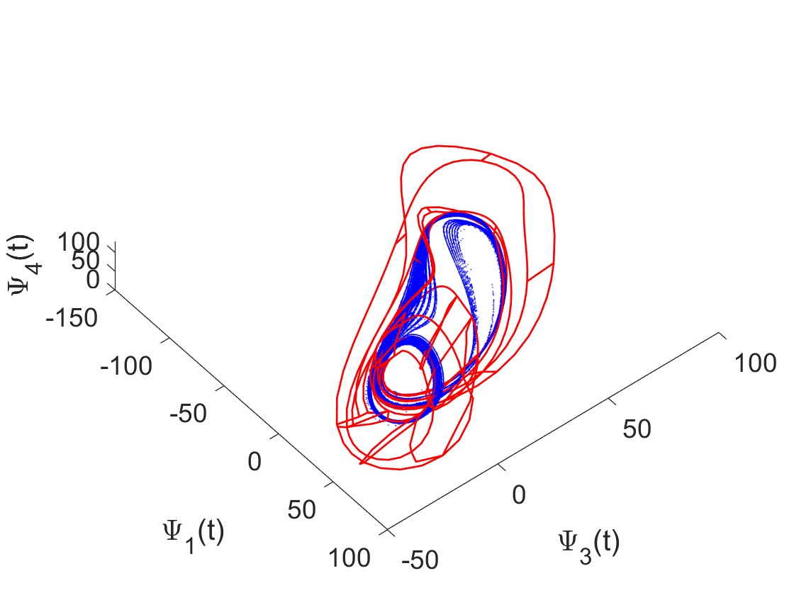
(b) $\mathcal{G}_{2}$, $\tau_{2}=[113.26,115.34]$ yrs, $|\tau_{2}|=2.08$ yrs.

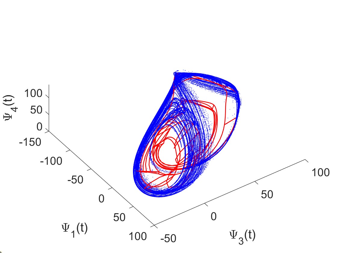
(c) $\mathcal{G}_{3}$, $\tau_{3}=[97.18,101.72]$ yrs, $|\tau_{3}|=4.54$ yrs.

(d) $\mathcal{G}_{4}$, $\tau_{4}=[108.2,110.15]$ yrs, $|\tau_{4}|=1.95$ yrs.

Figure 12: An ensemble of snapshots (in blue) juxtaposed with the cell complex for four different time windows $\tau_{i}$. The snapshots are evolving in distinct topological variability modes (TVMs): (a) TVM-1, (b) TVM-2, (c) TVM-3, and (d) TVM-4.

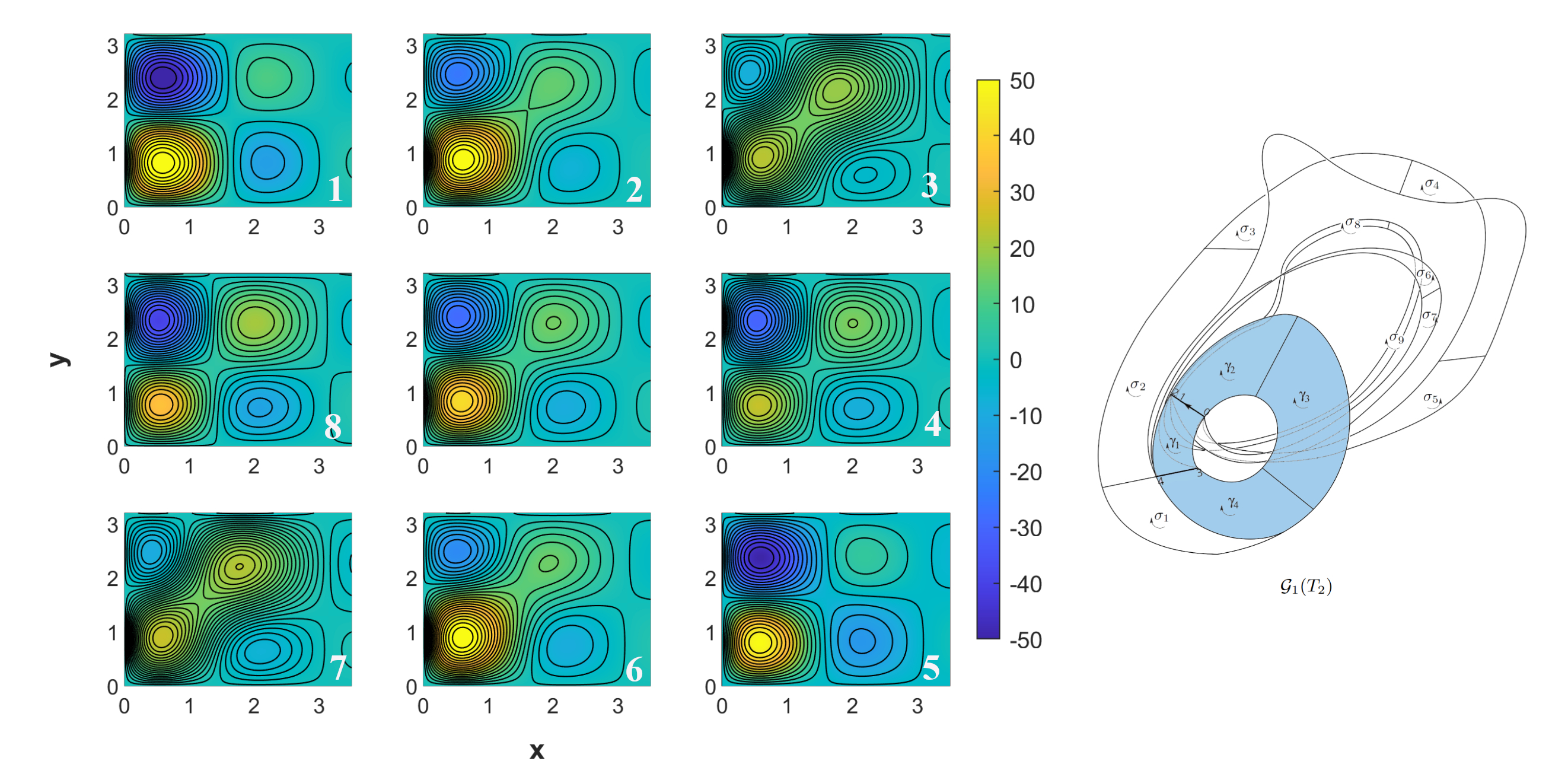
Figure 13: TVM-1 in physical space: a sequence of 8 snapshots (1–8) of $\psi=\psi(x,y,t)$ displayed in a circle around the central panel, which contains the mean $\overline{\psi(x,y)}$ of the TVM (left). TVM-1 in phase space corresponds to the generatex $\mathcal{G}_{1}$ (right). Note that the labels (1–8) on the left are in white on the dark background and are placed in the lower-right corner of each subpanel. The correspondence between the numbering of the subpanels on the left and the cells of the generatex on the right is the following: $\{1,5\}\to\gamma_{2}$, $\{2,6\}\to\gamma_{3}$, $\{3,7\}\to\gamma_{4}$, and $\{4,8\}\to\gamma_{1}$.

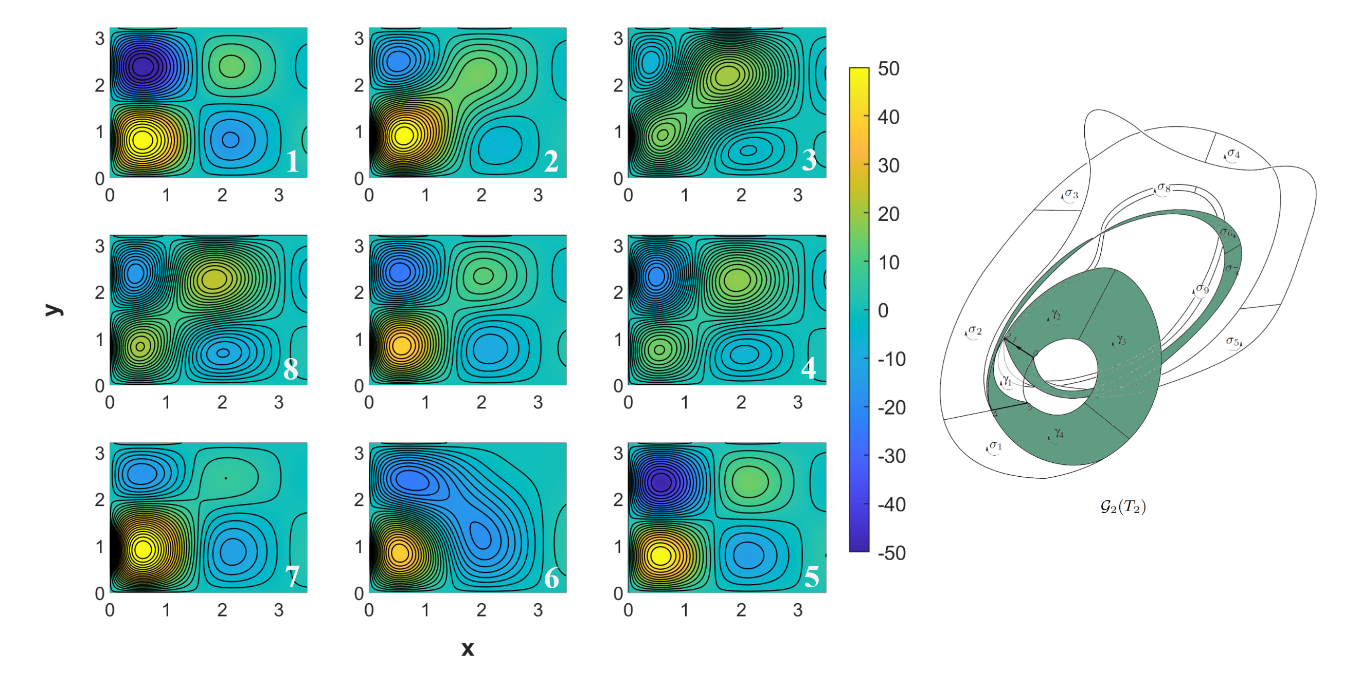
Figure 14: Same as Fig. 13, but for TVM-2 and $\mathcal{G}_{2}$. The correspondence between the numbering of the subpanels on the left and the cells of the generatex on the right is the following: $\{1\}\to\gamma_{2}$, $\{2\}\to\gamma_{3}$, $\{3\}\to\gamma_{4}$, $\{4,5,6\}\to\sigma_{6}$, and $\{7,8\}\to\sigma_{7}$.

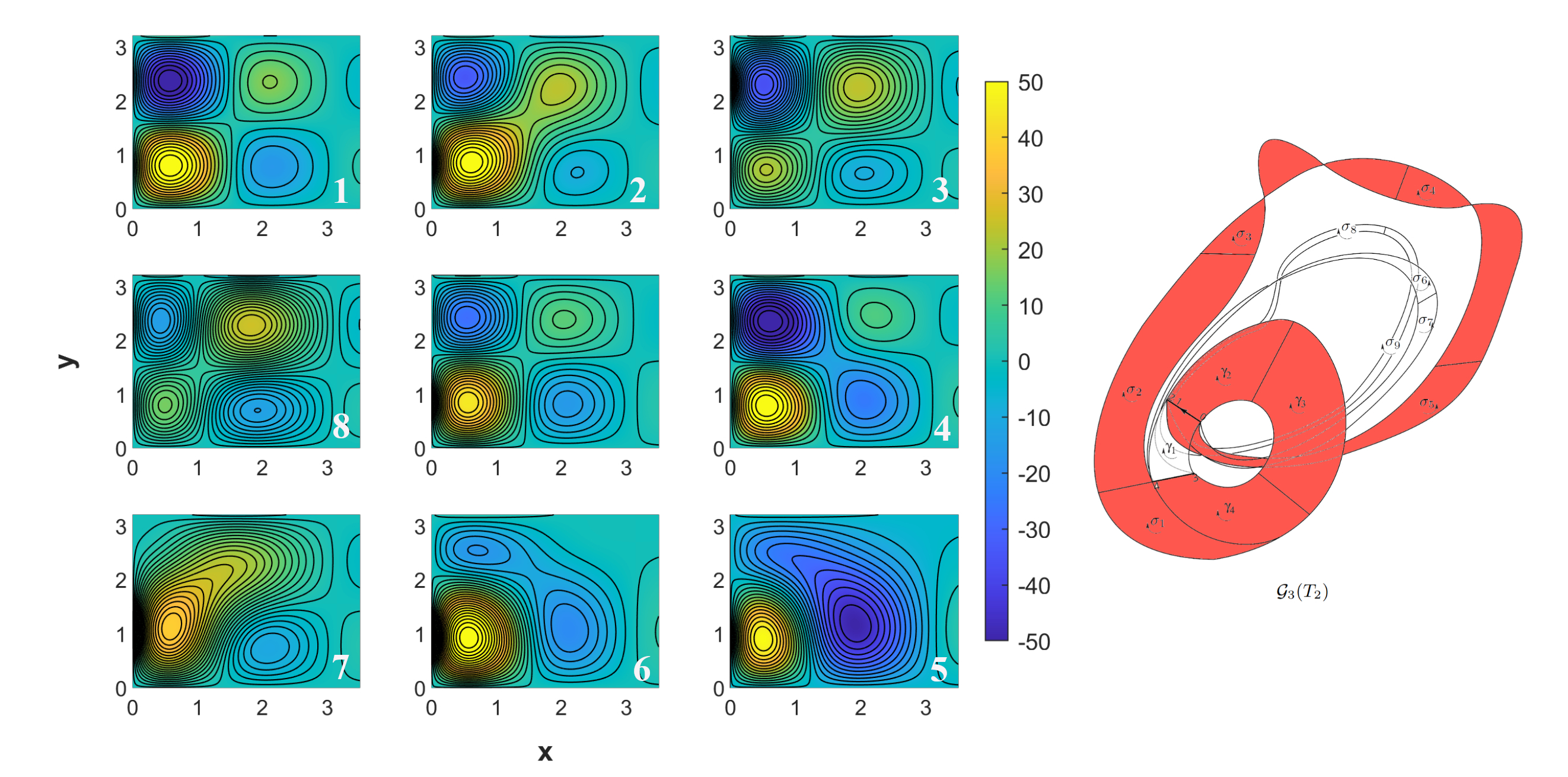
Figure 15: Same as Fig. 13, but for TVM-3 and $\mathcal{G}_{3}$. The correspondence between the numbering of the subpanels on the left and the cells of the generatex on the right is the following: $\{1\}\to\gamma_{2}$, $\{2\}\to\gamma_{3}$, $\{3\}\to\sigma_{1}$, $\{4\}\to\sigma_{2}$, $\{5\}\to\sigma_{3}$, $\{6\}\to\sigma_{4}$, and $\{7,8\}\to\sigma_{5}$ .

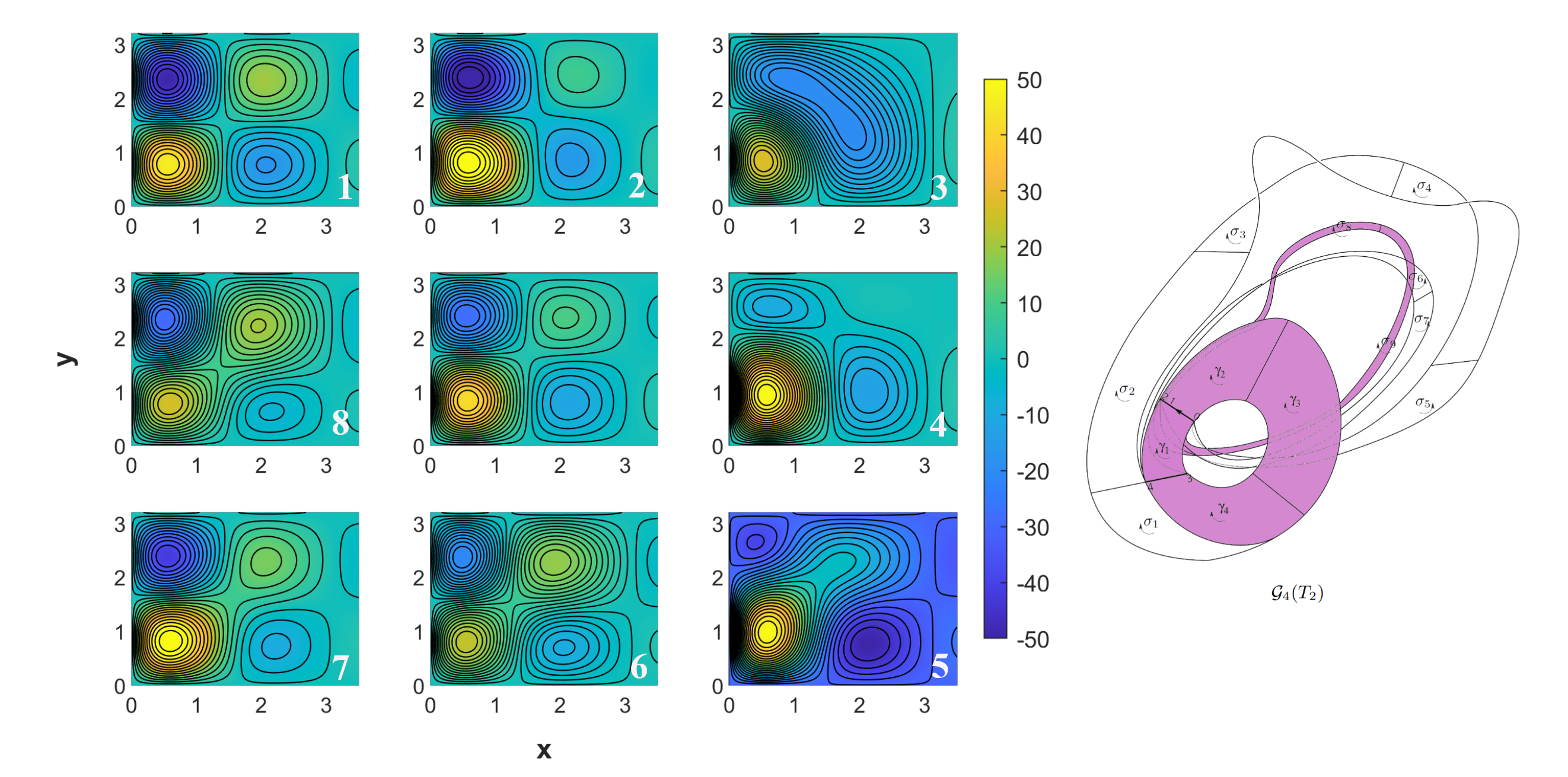
Figure 16: Same as Fig. 13, but for TVM-4 and $\mathcal{G}_{4}$. The correspondence between the numbering of the subpanels on the left and the cells of the generatex on the right is the following: $\{1,2,3\}\to\sigma_{8}$, $\{4,5,6\}\to\sigma_{9}$, $\{7\}\to\gamma_{3}$, and $\{8\}\to\gamma_{4}$

In order to accurately capture the nonlinearity of the dynamics, it is imperative to embed the data into a sufficiently high-dimensional phase space so as to avoid false neighbors. The regions of this phase space that are visited by the trajectories of the dynamical system can be represented by a branched manifold. This branched manifold will be approximated by a cell complex and the nonequivalent cycles of cells in this complex will represent distinguished paths in the phase space, i.e., the set of generatexes. In this section, we define a dynamical system’s topological variability modes (TVMs) as its set of generatexes.

Figure 12 shows the evolution of the snapshots through the four generatexes of the templex $T_{2}$ for four distinct time windows $\tau_{i}$. It is evident that the set of four generatexes results in a set of four TVMs: TVM-1, TVM-2, TVM-3, and TVM-4.

The durations of the four TVMs are calculated based on the time taken for a trajectory to pass through the corresponding generatex. The durations, in years, are as follows: TVM-1: $15.68$, TVM-2: $17.9$, TVM-3: $12.58$, and TVM-4: $17.64$; see Fig. 9. In Figures 13, 14, 15, and 16, the TVMs are represented in both the physical and phase space. Note that each snapshot of $\psi$ corresponds to a trajectory in phase space that travels around a generatex. For instance, in Figures 13 and 14, the snapshots 1, 2 ,3, and 4 of $\psi$ are pairwise fairly similar, since they correspond to trajectories that travel through the 3-cells $\gamma_{2}$, $\gamma_{3}$ and $\gamma_{4}$ in either case, while snapshots 5, 6, 7, and 8 exhibit marked differences between TVM-1 and TVM-2. The latter differences are attributable to the specific segment of the trajectory that corresponds to generatex. The captions provide the correspondence between the numbering of the subpanels on the left and the specific cells in the generatex on the right.

VI Concluding remarks

How can topology help describe the variability associated with dynamical modes in the climate system? The topological features captured by the templex reveal the nonlinear aspects of a system’s dynamics, providing a framework to investigate large-scale variability and predictability in both autonomous settings and nonautonomous ones.

In the present paper, we have shown how the BraMAH cell complex $K(A)$ can reveal important topological aspects of the branched manifold of a nonlinear, chaotic system $A$, and how these insights can be further enhanced by studying the associated digraph $G(A)$. Charó, Letellier, and Sciamarella (2022); Ghil and Sciamarella (2023). These concepts and the associated methodology for a templex ${\mathcal{T}}(A)=(K(A),G(A))$ were introduced in Sect. II.

In Sect. III, we introduced our highly idealized model of the wind-driven double-gyre ocean circulation, governed by four ordinary differential equations,Pierini, Ghil, and Chekroun (2016); Pierini, Chekroun, and Ghil (2018) and applied templex analysis to both an autonomous case, with wind stress curl constant in time, and a nonautonomous case, with periodic forcing. The latter corresponded to $T_{p}=30$ years, an interdecadal period approximating the irregular forcing used in Pierini, Ghil, and Chekroun (2016).

In Sect. IV, we clarified the necessary distinctions in the NDS literature as applied to the climate sciences between pullback (PBA) and forward (FWA), or snapshot, attractors, and computed our model’s snapshot attractor. After a convergence interval of roughly 66 years, the attractor became periodic, as expected, synchronizing with the forcing; see Figs. 9 and 10.

Finally, in Sect. V, we introduced the topological variability modes (TVMs) that are the main result of this paper. A dynamical system’s TVMs were defined to be its set of generatexes, and displayed for our idealized ocean model in both phase space and physical space; see Figs. 12 –16.

It is clear that TVMs are a truly novel decomposition mode of irregular flows that is based neither on statistics, like principal components Preisendorfer (1988); Jolliffe (2002), nor on Koopman operators Mezić (2013). It clearly requires many more applications to a variety of settings, in particular to higher dimensional ones. But the topological concepts and methods on which it rests are capable, at least in principle, to brave such tests.

It will be especially interesting to associate segments of trajectory in higher dimensional cases with the vicinity of joining loci of a generatex. Away from such vicinities, and in the absence of cells that belong to more than one generatex, the predictability of a trajectory is expected to be fairly high, while the contrary is to be expected when a cell belongs to more than one generatex or in the presence of a joining locus. Topological analysis of a dynamical system based on its BraMAH complex and on the associated digraph may thus lead to a totally new set of robust early warning signals.

Appendix A Homologies for a BraMAH complex

This appendix illustrates the construction of a BraMAH complex. Consider as an example a BraMAH complex $K(\mathbb{T}^{2})$ of dimension $2$ for a three-dimensional point cloud on a toroidal surface $\mathbb{T}^{2}$, as shown in Figure 17. We follow the definitions provided by Kinsey 2012 and the code in Sciamarella 2023 to show how the homologies are computed.

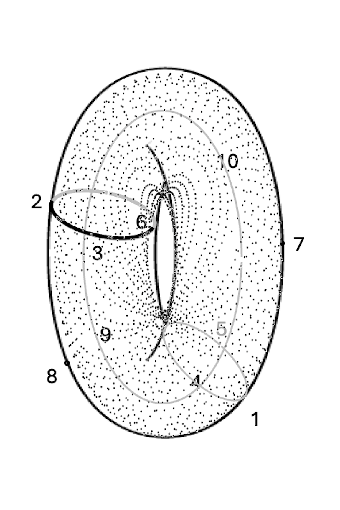
(a) (b)

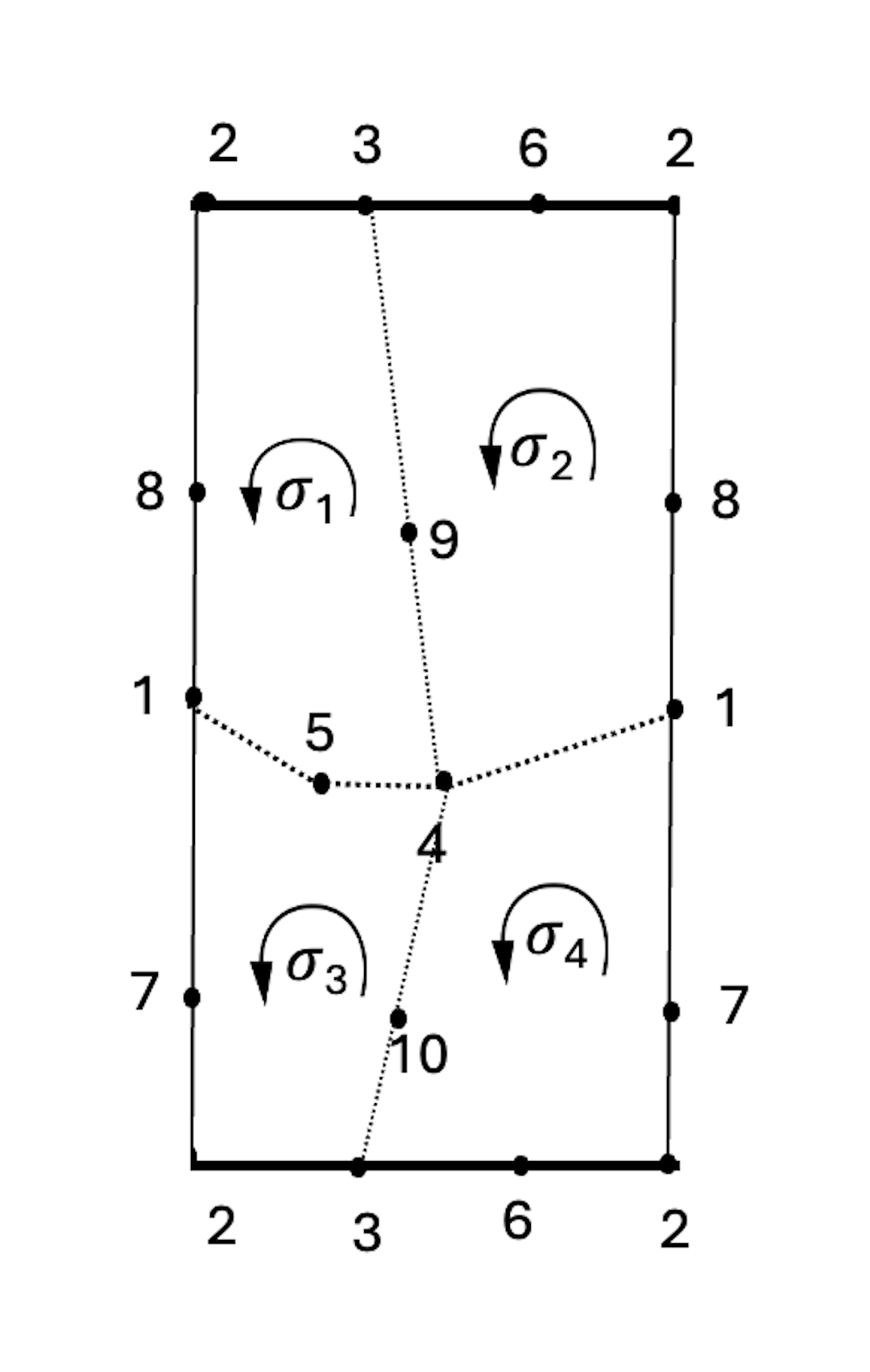
Figure 17: BraMAH cell complex for a torus. (a) A point cloud (gray dots) corresponding to a regular flow on a toroidal surface $\mathbb{T}^{2}$, with a BraMAH cell complex $K(\mathbb{T}^{2})$ sketched on it; and (b) a planar diagram of $K(\mathbb{T}^{2})$, where repeated labels indicate gluing. The anticlockwise orientation of $\sigma_{1}$ is propagated to the other 2-cells so as to make $K(\mathbb{T}^{2})$ be uniformly oriented.

Chain groups are algebraic structures that encode the $k$-dimensional features of a cell complex. The $k$-th chain group is denoted by $C_{k}(K)$ and it consists of all linear combinations of $k$-cells in the complex with integer coefficients. The chain groups of the cell complex $K(\mathbb{T}^{2})$ are as follows:

1. $C_{2}$: The group of 2-chains, generated by the 2-cells $\{\sigma_{1},\sigma_{2},\sigma_{3},\sigma_{4}\}$ with the orientations indicated in the planar diagram of Fig. 17(b).

2. $C_{1}$: The group of 1-chains, generated by the edges of the 2-cells in the complex. The edges, oriented from the lower-numbered to the higher-numbered vertices, include:

   $$\langle 1,4\rangle,\langle 1,5\rangle,\langle 1,7\rangle,\langle 1,8\rangle,\langle 2,3\rangle,\langle 2,7\rangle,\langle 2,8\rangle,\dots$$

3. $C_{0}$: The group of 0-chains, generated by the vertices $\{\langle 1\rangle,\langle 2\rangle,\langle 3\rangle,\langle 4\rangle,\dots\}$.

These groups represent collections of $k$-dimensional cells, and their relationships are described by the boundary operators. A boundary operator $\partial_{k}$ maps $k$-chains to $(k-1)$-chains, so that:

1. For a 1-cell $\langle 1,4\rangle$, the operator $\partial_{1}(\langle 1,4\rangle)$ is the difference of its terminal and initial vertices:

   $$\partial_{1}(\langle 1,4\rangle)=\langle 4\rangle-\langle 1\rangle.$$

2. For the 2-cell $\sigma_{2}$:

   $$\partial_{2}(\sigma_{2})=\langle 1,8\rangle-\langle 2,8\rangle\\ +\langle 2,6\rangle-\langle 3,6\rangle+\langle 3,9\rangle-\langle 4,9\rangle-\langle 1,4\rangle.$$

Note that the orientations of 1-cells and 2-cells are essential for applying the boundary operator. Consistent orientations can be assigned arbitrarily, as long as they are respected throughout the computation.

Homology groups are defined as:

$$H_{k}(K)=\ker(\partial_{k})/\operatorname{im}(\partial_{k+1};$$

here $\ker(\partial_{k})$ is the group of cycles, i.e., of chains whose boundaries are zero, and $\operatorname{im}(\partial_{k+1})$ is the group of boundaries, i.e., of chains that are boundaries of $(k+1)$-chains.

The $k$-th Betti number, denoted by $\beta_{k}$, is the rank of the $k$-th homology group. In other words, $\beta_{k}$ corresponds to the number of independent $k$-dimensional cycles in the complex:

$$\beta_{k}=\text{rank}(H_{k}(K)).$$

For the cell complex $K(\mathbb{T}^{2})$ in Figure 17, we compute the homology groups and Betti numbers, and explicitly describe the generators as follows:

1. The 0th homology group represents the connected components of the manifold underlying the point cloud. The generator of $H_{0}(K(\mathbb{T}^{2}))$ corresponds to any of the 0-cells, since all of them are homologous:

   $$g_{0_{1}}=\langle 1\rangle.$$

   We thus write:

   $$H_{0}(K(\mathbb{T}^{2}))=[[g_{0_{1}}]]\simeq\mathbb{Z},\quad\beta_{0}=1.$$

2. The 1st homology group captures homologically independent nontrivial loops. The torus has two:

   1. A poloidal loop, aligned with the shortest circle on the surface, represented by:

      $$g_{1_{1}}=\langle 2,3\rangle+\langle 3,6\rangle-\langle 2,6\rangle.$$

   2. A toroidal loop around the central axis of the torus, represented by:

      $$g_{1_{2}}=\langle 1,7\rangle-\langle 2,7\rangle+\langle 2,8\rangle-\langle 1,8\rangle.$$

   We thus write:

   $$H_{1}(K(\mathbb{T}^{2}))=[[g_{1_{1}},g_{1_{2}}]]\simeq\mathbb{Z}^{2},\quad\beta_{1}=2.$$

3. The 2nd homology group captures enclosed cavities. The torus encloses a single cavity, and the 2-generator is:

   $$g_{2_{1}}=\sigma_{1}+\sigma_{2}+\sigma_{3}+\sigma_{4}.$$

   We thus write:

   $$H_{2}(K(\mathbb{T}^{2}))=[[g_{2_{1}}]]\simeq\mathbb{Z},\quad\beta_{2}=1.$$

If the 0-cells along the bottom line of the planar diagram of Figure 17(b) that are labeled $2,3,6,2$ are relabeled $2,6,3,2$, modifying thus the gluing instructions, the torus becomes a Klein bottle $\mathbb{K}^{2}$. While the 2-cells $\sigma_{1}$ and $\sigma_{2}$ remain the same, the 2-cells below them become $\sigma_{3}=\langle 2,6,10,4,5,1,7\rangle$ and $\sigma_{4}=\langle 1,4,10,6,3,2,7\rangle$. Computing homologies for this new complex, we still have $\beta_{0}=1$, but $\beta_{1}=1$ and $\beta_{2}=0$, i.e., there is no longer an enclosed cavity. The torsion group is given by the 1-chain forming the nonorientable cycle:

$$-2\langle 2,3\rangle-2\langle 3,6\rangle+2\langle 2,6\rangle.$$

The Klein bottle is said to have a weak boundary because its nonorientable structure implies that 1-cycles fail to bound 2-chains in a consistent manner. Specifically, the torsion group reflects this property.

We have thus shown how building a BraMAH cell complex is useful in computing the topological properties of the manifold underlying a point cloud.

Data availability

The Wolfram Mathematica code to compute homology groups and templex properties with examples are available at https://git.cima.fcen.uba.ar/sciamarella/bramah_torus/ and https://git.cima.fcen.uba.ar/sciamarella/templex-properties or https://community.wolfram.com/groups/-/m/t/3079776.

References

References

- Ghil and Lucarini (2020) M. Ghil and V. Lucarini, “The physics of climate variability and climate change,” Reviews of Modern Physics 92, 035002 (2020).
- Veronis (1963) G. Veronis, “An analysis of wind-driven ocean circulation with a limited number of fourier components,” Journal of Atmospheric Sciences 20, 577–593 (1963).
- Jiang, Jin, and Ghil (1995) S. Jiang, F.-F. Jin, and M. Ghil, “Multiple equilibria, periodic, and aperiodic solutions in a wind-driven, double-gyre, shallow-water model,” Journal of physical oceanography 25, 764–786 (1995).
- Ghil and Childress (2012) M. Ghil and S. Childress, Topics in Geophysical Fluid Dynamics: Atmospheric Dynamics, Dynamo Theory, and Climate Dynamics (Springer, 1987, reissued, 2012).