Conformal novelty detection for replicate point patterns with FDR or FWER control

Abstract

Monte Carlo tests are widely used for computing valid p-values without requiring known distributions of test statistics. When performing multiple Monte Carlo tests, it is essential to maintain control of the type I error. Some techniques for multiplicity control pose requirements on the joint distribution of the p-values, for instance independence, which can be computationally intensive to achieve using naïve multiple Monte Carlo testing. We highlight in this work that multiple Monte Carlo testing is an instance of conformal novelty detection. Leveraging this insight enables a more efficient multiple Monte Carlo testing procedure, avoiding excessive simulations while still ensuring exact control over the false discovery rate or the family-wise error rate. We call this approach conformal multiple Monte Carlo testing. The performance is investigated in the context of global envelope tests for point pattern data through a simulation study and an application to a sweat gland data set. Results reveal that with a fixed number of simulations under the null hypothesis, our proposed method yields substantial improvements in power of the testing procedure as compared to the naïve multiple Monte Carlo testing procedure.

Keywords: multiple hypothesis testing, global envelope tests, spatial statistics, Monte Carlo tests, point processes

1 Introduction

We study a novelty detection problem where we have access to a null sample $\mathcal{D}^{\rm null}=\{\boldsymbol{X}_{i}\}_{i=1}^{n}$ of independent data points generated under a distribution $P_{0}$ on a space $\mathcal{X}$, and a test sample $\mathcal{D}^{\rm test}=\{\boldsymbol{X}_{n+j}\}_{j=1}^{m}$ where $\boldsymbol{X}_{n+j}\sim P_{j}$ for a distribution $P_{j}$ on the space $\mathcal{X}$, for $j=1,\dots,m$. We call each $\boldsymbol{X}_{n+j}$ a test point, and consider specifically the case where $\mathcal{X}$ is the space of locally finite point configurations on a bounded domain. There the aim is to test which observations in $\mathcal{D}^{\rm test}$ are novelties, i.e. $P_{j}\neq P_{0}$, for $j=1,\dots,m$, while controlling for false positives that can be extremely harmful in practice.

This setting is common in spatial statistics where we encounter replicated point pattern data (Diggle et al. (2000)). Examples are locations of pyramidal neurons (Diggle et al. (1991)), cells (Baddeley et al. (1993)), epidermal nerve fibers (Konstantinou et al. (2023)), sweat glands (Kuronen et al. (2021)), and more (Baddeley et al. (2015)). For instance the sweat gland data studied by Kuronen et al. (2021) consisting in five point patterns for each of the following three groups of subjects: diagnosed with neuropathy, suspected to have neuropathy, control (assumed to not have neuropathy). In this case, we would be interested in deriving a multiple testing procedure for the subjects suspected to have neuropathy, based on the data from the control subjects and the diagnosed subjects.

Our setting can be compared to the ones of Gandy & Hahn (2014, 2017), and Hahn (2020), although we differ in part due to our focus on spatial data. There, for each $j$, testing for $P_{j}\neq P_{0}$ is done by Monte Carlo tests which are based on a null sample constructed from independent simulations under $P_{0}$, see Baddeley et al. (2015) and Myllymäki et al. (2017). This results in independent $p$-values, and procedures such as the Hochberg procedure by Hochberg (1988) or the Benjamini-Hochberg procedure by Benjamini & Hochberg (1995) can be used to ensure bounds on the family-wise error rate (FWER) or the false discovery rate (FDR), respectively. However, this comes with a significant computational strain, in particular if the number of test points $m$ is large and simulation under $P_{0}$ difficult, as for each $j=1,\ldots,m$ we need to have access to a new null sample.

Adopting another approach, Bates et al. (2023) and Marandon et al. (2024) re-use simulations under $P_{0}$ for different test points thereby resulting in dependent $p$-values which in general cannot control the FWER or the FDR. In particular, Bates et al. (2023) introduced conformal $p$-values, and proved that they are positive regression dependent on a subset (PRDS), controlling the FDR under the Benjamini-Hochberg (BH) procedure (Benjamini & Yekutieli (2001). Further, they proved that the BH procedure with Storey’s correction (Storey (2002); Storey et al. (2004)) also controls the FDR.

Inspired by this approach, we propose a conformal multiple Monte Carlo testing procedure based on a single null sample. Our method significantly reduces the computational burden with respect to the standard multiple Monte Carlo approach. It is based on conformal $p$-values computed for each test point in $\mathcal{D}^{\rm test}$ which are then combined by Storey’s BH procedure (resp. the Hochberg procedure). Using recent advances of conformal novelty detection in Bates et al. (2023) and Marandon et al. (2024), we prove that the methods control the FDR (resp. the FWER) and present a rigorous procedure for testing goodness-of-fit for replicate point patterns. In doing so we extend the global envelope tests in Myllymäki et al. (2017) to replicate point patterns, while highlighting connections between conformal methodology and Barnard’s Monte Carlo test (Barnard (1963)). On simulated data and a dataset from biology on the position of sweat glands among patients with neuropathy, we illustrate that our method significantly improves the power of testing procedures for replicate point patterns, compared to a naïve usage of Myllymäki et al. (2017).

The rest of the paper is organized as follows. Section 2 presents preliminaries on multiple testing as well as the recent developments surrounding conformal $p$-values, and we present in Section 3 our contribution to FWER control with conformal $p$-values. Then, Section 4 outlines how conformal $p$-values can be used for multiple testing in the context of spatial point processes, herein relating conformal novelty detection to the modern global envelope tests in the domain of spatial statistics. Section 5 presents simulation studies illustrating the power of the proposed methodology, and in Section 6, we apply it to the sweat gland data from Kuronen et al. (2021). Finally, Section 7 concludes the paper and presents some future research directions.

2 Background

2.1 Multiple hypothesis testing

We consider the multiple hypothesis testing scenario in which $m$ test points are observed and a null hypothesis is tested on each of them. In other words, $m$ null hypotheses $H^{1}_{0},\dots,H^{m}_{0}$ are tested at level $q^{*}\in(0,1)$, and we denote by $p_{1},\dots,p_{m}$ the corresponding $p$-values.

We denote by $S$ the number of rejected non-true null hypotheses, and by $V$ the number of rejected true null hypotheses (type I error). Moreover, $\mathcal{R}=V+S$ denotes the total number of rejected hypotheses, while $m_{0}$ denotes the number of true null hypotheses.

A classical error rate studied for multiple comparisons is the FDR criterion, proposed by Benjamini & Hochberg (1995), which is defined as $\mathrm{FDR}=\mathbb{E}[\mathrm{FDP}]$, where $\mathrm{FDP}~=~V/\max(1,\mathcal{R})$. The power of a test, also called the true discovery rate (TDR), is defined as $\mathbb{E}[{\rm TDP}]$, where the true discovery proportion is ${\rm TDP}=S/\max(1,m-m_{0})$. The most known method to control the FDR is the BH procedure presented below.

Definition 1 (BH procedure (Benjamini & Hochberg (1995))).

Let $p_{(1)}\leq p_{(2)}\leq\cdots\leq p_{(m)}$ be the ordered $p$-values and denote by $H^{(j)}_{0}$ the null hypothesis associated to $p_{(j)}$. The BH procedure with level $q^{*}\in(0,1)$ is to reject $H^{(1)}_{0},\dots,H^{(k)}_{0}$ where

$$k=\max_{j\in\{1,\dots,m\}}\Big{\{}p_{(j)}\leq\frac{j}{m}q^{*}\Big{\}}.$$

When the $p$-values are independent, the BH procedure controls the FDR at level $\pi_{0}q^{*}$ where $\pi_{0}=m_{0}/m$ is the proportion of true nulls, see Benjamini & Hochberg (1995). We present below a more general condition under which the BH procedure also controls the FDR at level $\pi_{0}q^{*}$, namely PRDS.

Definition 2 (PRDS (Benjamini & Yekutieli (2001))).

A random vector $\boldsymbol{X}=(X_{i})_{i=1\dots m}$ is PRDS on $\mathcal{H}_{0}\subset\{1,\dots,m\}$ if for any increasing set $\mathcal{D}$, i.e., that $x\in\mathcal{D}$ and $x\leq y$ implies $y\in\mathcal{D}$, and for each $i\in\mathcal{H}_{0}$, the function $\mathbb{P}(\boldsymbol{X}\in\mathcal{D}|X_{i}=x)$ is nondecreasing in $x$.

Theorem 1 (Theorem 1.2 (Benjamini & Yekutieli (2001))).

If the joint distribution of $p$-values is PRDS on $\mathcal{H}_{0}=\{j\in\{1,\dots,m\}\;\mathrm{s.t.}\;H_{0}^{j}\;\mathrm{is}\;\mathrm{true}\}$, then the BH procedure applied with level $q^{*}\in(0,1)$ controls the FDR at level less than or equal to $\pi_{0}q^{*}$:

$${\rm FDR}=\mathbb{E}\bigg{(}\frac{V}{\max(1,\mathcal{R})}\bigg{)}\leq\pi_{0}q^{*}\leq q^{*}.$$

To avoid being overly conservative, we would need to know $\pi_{0}$ and set $q^{*}=\alpha/\pi_{0}$ to have global significance level $\alpha\in(0,1)$. However, in practice $\pi_{0}$ is not known, and several estimation procedures have been proposed (see e.g. Storey (2002), Storey et al. (2004) and Benjamini et al. (2006)), without one being constantly better. We present below the Storey estimator as it adapts well in our conformal inference setting (see Theorem 3).

Definition 3 (Storey’s estimator (Storey et al. (2004))).

The Storey estimator of the proportion of true nulls $\pi_{0}$ with parameter $\lambda\in[0,1)$ is

$$\hat{\pi}_{0}=\frac{1+\sum_{i=1}^{m}\mathbbm{1}[p_{i}>\lambda]}{m(1-\lambda)}.$$

The idea is that the $p$-values contain information regarding the number of true null hypotheses among the $m$ hypotheses. The hyper-parameter $\lambda$ has a classic influence on $\hat{\pi}_{0}$ in terms of bias-variance trade-off. A bootstrap procedure for choosing the optimal $\lambda$ is proposed by Storey (2002) in the case of independent $p$-values, but in general, the BH procedure used with an estimator of $\pi_{0}$ does not control the FDR at the prescribed level in case of PRDS $p$-values. We present in Section 2.2 how conformal $p$-values, used in combination with Storey’s estimator from Definition 3 allows to control the FDR.

A different error criterion for multiple testing which is more strict than FDR is the FWER, defined as $\mathbb{P}(V\geq 1)$. The traditional Bonferroni procedure for controlling the FWER is to reject any hypothesis $H^{j}_{0}$, $j=1,\dots,m$, for which the corresponding $p$-value $p_{j}\leq q^{*}/m$ for significance level $q^{*}\in(0,1)$ (Bonferroni (1936)). Equipped with a liberal estimator of $\hat{m}_{0}$, for instance Storey’s estimator, a sharper Bonferroni procedure is to reject when $p_{j}\leq q^{*}/\hat{m}_{0}$. Multiple testing procedures for controlling the FWER, which are uniformly more powerful than the traditional Bonferroni procedure, have been proposed under certain dependency requirements, for instance the Hochberg procedure presented below (Simes (1986); Hochberg (1988)).

Definition 4 (Hochberg procedure (Hochberg (1988))).

Let $p_{(1)}\leq p_{(2)}\leq\cdots\leq p_{(m)}$ be the ordered $p$-values and denote by $H^{(j)}_{0}$ the null hypothesis associated to $p_{(j)}$. The Hochberg procedure with level $q^{*}\in(0,1)$ is to reject $H^{(1)}_{0},\dots,H^{(k)}_{0}$ where

$$k=\max_{j\in\{1,\dots,m\}}\Big{\{}p_{(j)}\leq\frac{q^{*}}{m-j+1}\Big{\}}.$$

The Hochberg procedure controls the FWER at level $q^{*}\in(0,1)$ when the $p$-values are independent, or when their joint distribution has a specific type of positive dependence called multivariate totally positive of order two (${\rm MTP}_{2}$, see Definition 6) (Sarkar & Chang (1997); Sarkar (1998)).

2.2 Conformal p-values

A conformal inference approach to novelty detection has been studied in recent works under different names, see Bates et al. (2023); Mary & Roquain (2022); Marandon et al. (2024). The central assumption there is that the random variables in $\mathcal{D}^{\rm null}$ are exchangeable as defined below.

Definition 5 (Exchangeability).

The random variables $\boldsymbol{X}_{1},\dots,\boldsymbol{X}_{n}$ are exchangeable if their joint distribution is invariant by permutations.

Let $\hat{s}$ be a data driven score function mapping from $\mathcal{X}\times\mathcal{X}^{n+m}$ to a scalar set. The space $\mathcal{X}$ is traditionally $\mathbb{R}^{d}$ or $\mathbb{R}^{d\times d^{\prime}}$, see for instance Marandon et al. (2024), but in this work $\mathcal{X}$ will be the space of locally finite point configurations on a bounded domain. As usual in the conformal framework, this score is data driven and we will be particularly interested, for each $\boldsymbol{X}_{i}\in\mathcal{D}^{\rm null}\cup\mathcal{D}^{\rm test}$, in the evaluation of $\hat{s}_{i}=\hat{s}(\boldsymbol{X}_{i},(\boldsymbol{X}_{1},\dots,\boldsymbol{X}_{n+m}))$. We denote by $\mathcal{H}_{0}=\{j\in\{1,\dots,m\}\;\mathrm{s.t.}\;H_{0}^{j}\;\mathrm{is}\;\mathrm{true}\}$ the set of nulls in the test sample $\mathcal{D}^{\rm test}$, $\mathcal{H}_{1}=\{1,\dots,m\}\setminus\mathcal{H}_{0}$, and make the following assumptions on the score and the data:

1. for any permutation $\pi$ of $\{1,\dots,n+m\}$, $\hat{s}$ satisfies for any $(\boldsymbol{X}_{1},\dots,\boldsymbol{X}_{n+m})\in\mathcal{X}^{n+m}$ the invariance property $\hat{s}(\cdot,(\boldsymbol{X}_{\pi(1)},\dots,\boldsymbol{X}_{\pi(n+m)}))=\hat{s}(\cdot,(\boldsymbol{X}_{1},\dots,\boldsymbol{X}_{n+m}))\,;$

2. $(\boldsymbol{X}_{1},\dots,\boldsymbol{X}_{n},(\boldsymbol{X}_{n+i})_{i\in\mathcal{H}_{0}})$ are exchangeable conditional on $(\boldsymbol{X}_{n+i})_{i\in\mathcal{H}_{1}}$;

3. there are almost surely no ties among $(\hat{s}_{1},\ldots,\hat{s}_{n+m})$, i.e., $\mathbb{P}(\hat{s}_{i}<\hat{s}_{j}\lor\hat{s}_{j}<\hat{s}_{i})=1$ for all $i\neq j$.

For $j=1,\ldots,m$, we define the conformal $p$-value associated to the test point $\boldsymbol{X}_{n+j}$ by

$$\hat{p}_{j}=\frac{1}{n+1}\Big{(}1+\sum_{i={1}}^{n}\mathbbm{1}[\hat{s}_{i}\leq\hat{s}_{n+j}]\Big{)}.$$ (1)

The conformal framework can be extended to conformal scores $\hat{s}$ taking values in a non-scalar space equipped with an ordering $\preceq$. Then, the p-values can be defined as (1) with $\leq$ replaced by $\preceq$ (Myllymäki et al. (2017)).

Notice that Marandon et al. (2024) exposes a more general case where the score function is learned: the null sample $\mathcal{D}^{\rm null}$ is then split in two parts $(\boldsymbol{X}_{1},\dots,\boldsymbol{X}_{\ell})$ and $(\boldsymbol{X}_{\ell+1},\dots,\boldsymbol{X}_{n+m})$, where the former is used only for learning $\hat{s}$, and the invariance assumption ($\mathcal{A}$1) becomes

$$\hat{s}(\cdot,(\boldsymbol{X}_{1},\dots,\boldsymbol{X}_{\ell}),(\boldsymbol{X}_{\pi(\ell+1)},\dots,\boldsymbol{X}_{\pi(n+m)}))=\hat{s}(\cdot,(\boldsymbol{X}_{1},\dots,\boldsymbol{X}_{\ell}),(\boldsymbol{X}_{\ell+1},\dots,\boldsymbol{X}_{n+m}))\,,$$

and the conformal $p$-values are given by $\hat{p}_{j}=\frac{1}{n-\ell+1}\big{(}1+\sum_{i=\ell+1}^{n}\mathbbm{1}[\hat{s}_{i}\leq\hat{s}_{n+j}]\big{)}$. In Section 4, we view conformal novelty detection in the context of global envelope tests for replicate point patterns, and here we do not need $\ell>0$, so for the sake of readability we consider hereinafter $\ell=0$. As shown first by Bates et al. (2023) for $\ell=0$ and extended to the case $\ell\geq 0$ by Marandon et al. (2024), conformal $p$-values from (1) are PRDS, which implies that applying BH procedure (Definition 1) controls the FDR. Furthermore, Marandon et al. (2024) have proved a lower bound for FDR, as stated in the theorem below.

Theorem 2 (FDR control (Marandon et al. (2024))).

Let assumptions ($\mathcal{A}$1)-($\mathcal{A}$3) be true for a conformal score $\hat{s}$. The BH procedure (see Definition 1) at level $q^{*}$ with the conformal $p$-values satisfies

$$m_{0}\frac{\lfloor q^{*}(n-1)/m\rfloor}{(n-1)}\leq\mathbb{E}\left(\frac{V}{\max(1,\mathcal{R})}\right)\leq\pi_{0}q^{*},$$

and

$$\mathbb{E}\left(\frac{V}{\max(1,\mathcal{R})}\right)=\pi_{0}q^{*},$$

when $q^{*}(n+1)/m$ is an integer.

Moreover, Bates et al. (2023) showed that the FDR is controlled in the case of Storey’s correction, which we state in Theorem 3 below.

Theorem 3 (Storey’s BH with conformal $p$-values (Bates et al. (2023); Marandon et al. (2024))).

Let $\hat{p}_{j}$, for $j=1,\ldots,m$, be conformal $p$-values given by (1) with a conformal score verifying ($\mathcal{A}$1)-($\mathcal{A}$3). Let further $\hat{\pi}_{0}$ be Storey’s estimator as in Definition 3. Then, the BH procedure, as in Definition 1, applied at level $q^{*}=\alpha/\hat{\pi}_{0}$ to $\hat{p}_{1},\ldots,\hat{p}_{m}$ controls the FDR at the prescribed significance level $\alpha\in(0,1)$.

3 Controlling the FWER with conformal p-values

While FDR is a more common and popular multiple testing criterion, some situations still warrants the use of the FWER, i.e., in cases where a practitioner is really interested in controlling the probability of making one or more false rejections.

Angelopoulos et al. (2024) highlighted through Proposition 10.2 that a Bonferroni-type procedure rejecting hypothesis $j$ when $p_{j}\leq 1-(1-\alpha)^{1/m}$ for significance level $\alpha\in(0,1)$ controls the FWER at the nominal level, and that asymptotically as the size of the null sample $n$ increases, the FWER converges exactly to $\alpha$. Yet, it would be reasonable to expect that one could construct a more powerful procedure in the case of finite $n$ which does not use a constant threshold for all $p$-values, but instead uses a sequence of thresholds on the ordered $p$-values.

It was shown by Gazin et al. (2024) that the joint probability mass function of the conformal $p$-values is

$$\mathbb{P}(\hat{\boldsymbol{p}}=\boldsymbol{j}/(n+1))=\frac{n!}{(n+m)!}\prod_{k=1}^{n+1}M_{k}(\boldsymbol{j})!,$$ (2)

for $\boldsymbol{j}\in\{1,\dots,n+1\}^{m}$ and where $M_{k}(\boldsymbol{j})=|\{i\in\{1,\dots,m\}:j_{i}=k\}|$.

We recall that if the joint distribution of $p$-values is ${\rm MTP}_{2}$, then the Hochberg procedure, see 4, controls the FWER. Since conformal $p$-values are positively correlated (Lemma 1 of Bates et al. (2023)) and ${\rm MTP}_{2}$ is a quite large class of distributions (Sarkar & Chang (1997)), one could expect that conformal $p$-values are ${\rm MTP}_{2}$. In the supplementary material, we show that this is not the case through a counter example based on the explicit form (2) (see Theorem 5 ). Still, we conjecture below, and proceed to show numerically, that the FWER can indeed be controlled with the Hochberg procedure when using conformal $p$-values.

Conjecture.

Let assumptions ($\mathcal{A}$1)-($\mathcal{A}$3) be true for a conformal score $\hat{s}$. Then, the Hochberg procedure (See Definition 4) at level $\alpha$ with the conformal $p$-values satisfies

$${\rm FWER}=\mathbb{P}(V\geq 1)\leq\alpha.$$

Remark 1.

In the supplementary material, we show that the joint distribution of the ordered $p$-values is uniform on an integer order set, see Lemma 1. Moreover, Lemma 3 in the supplementary material allows for a simple recursive expression for the ${\rm FWER}$, representing a computationally efficient way to numerically evaluate the ${\rm FWER}$. We prove also that the conjecture is true for $m=1,\dots,5$ (see Theorem 6), thereby covering all the cases considered in the numerical experiments part of this paper. Yet, a proof for all $m\geq 1$ has eluded the authors.

Using Lemma 3 in the supplementary material, we can numerically compute the theoretical ${\rm FWER}$ for any sequence of thresholds applied on the ordered $p$-values. We show then in Figure 1 the ${\rm FWER}$, for a scenario with $m=10$ and $m_{0}=5$ where the $m_{0}$ largest p-values are the true nulls, for significance levels $\alpha=0.05,0.1$, with the Hochberg procedure and the Bonferroni-type procedure rejecting at level $1-(1-\alpha)^{1/\hat{m}_{0}}$ with $\hat{m_{0}}=m_{0}$ and $\hat{m_{0}}=m_{0}+1$, against the null sample size, $n$. Here an estimator of $m_{0}$ is used to sharpen the Bonferroni-type procedure, and as for the traditional Bonferroni procedure this maintains FWER control assuming a liberal estimator of $m_{0}$ is used, such as Storey’s estimator Storey et al. (2004). Figure 1 shows the conservativeness of the Hochberg procedure for conformal p-values. Moreover, it highlights that the Hochberg procedure is not always better than the Bonferroni-type procedure, and vice versa. The over-conservativeness of the Bonferroni-type procedure is highly dependent on the quality of the estimator $\hat{m}_{0}$, while for Hochberg it depends on the order position of the true nulls. We conjecture that a procedure which is uniformly more powerful than both the Bonferroni-type procedure and the Hochberg procedure exists, and leave this as a problem for future investigation.

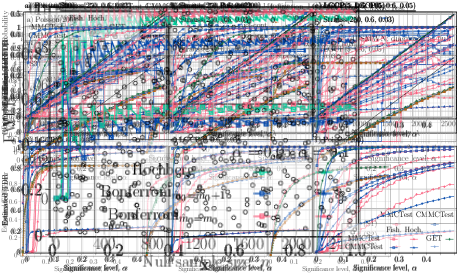
Figure 1: ${\rm FWER}$ against the null sample size, $n$.

4 Application to spatial point patterns

4.1 Point patterns and global envelope tests

Spatial points processes are used in various fields such as ecology, social sciences or biology to study the spatial distribution and interaction between objects/events of interest, trees, or cells, see Baddeley et al. (2015).

Mathematically, a point process is a random configuration of points such that in any bounded set there is almost surely a finite number of points. Alternatively, one can see a point process $\boldsymbol{X}$ as a random set $\{Z_{1},\ldots,Z_{N}\}$ where $N$ is an integer valued random variable, possibly infinite. For a rigorous mathematical presentation on point processes, we refer the reader to Last & Penrose (2017).

Due to their complex nature, relevant statistics for point processes that could be used for novelty detection are not scalar but functions, which often depends on the inter point distance, e.g., Besag’s $L$-function or Ripley’s $K$-function (see e.g. Møller & Waagepetersen (2004)). The problem with constructing tests based on such functional statistics is that one would need to conduct a global test for each inter point distance in a set of discretization points which requires either a multiple testing procedure or to reduce the functional statistic to a scalar. Examples of such methods are the maximum absolute deviation (MAD) test and the Diggle-Cressie-Loosmore-Ford (DCLF) test which are respectively adaptations of Kolmogorov-Smirnoff tests and Cramér-Von Mises tests to spatial statistics (Baddeley et al. (2015)). However, this drastically reduce the power of the tests we could define. A modern approach to tackle goodness-of-fit for point patterns is based on a functional version of Barnard’s Monte Carlo test, called global envelope test (Myllymäki et al. (2017)). A comprehensive review on goodness-of-fit tests for spatial point processes is given by Fend & Redenbach (2025).

Barnard’s Monte Carlo (Barnard (1963)) test can be summed up as following. Consider a statistic $T_{n+1}$ associated to the test point on which we want to test the goodness-of-fit of a null model $P_{0}$, and $n$ independent and identically distributed (iid) statistics $T_{1},\dots,\,T_{n}$, computed from $n$ iid points simulated under $P_{0}$. Recall that each data point in this setup is a point pattern. Under the null hypothesis, $T_{1},\dots,T_{n+1}$ are iid and $T_{n+1}$ is among the $\lfloor\alpha(n+1)\rfloor$ largest $T_{i}$ with probability $\alpha$. Notice that the distribution of the $T_{i}$ does not need to be known. Moreover, as in the conformal framework, we can replace the iid assumption by exchangeability of $T_{1},\dots,\,T_{n+1}$.

In global envelope tests, $T_{i}$ are functional statistics, typically the $L$-function. Applying the above methodology requires then to define an order relation between the $T_{i}$. In Myllymäki et al. (2017), the rank measure is defined as follows. Consider $\boldsymbol{X}_{1},\dots,\boldsymbol{X}_{n}$ iid from a null distribution $P_{0}$, and $\boldsymbol{X}_{n+1}$ a test point for which we want to test if $\boldsymbol{X}_{n+1}\sim P_{0}$. Let $T_{i}$ be a functional summary statistic for the point pattern $\boldsymbol{X}_{i}$ defined on an interval $I\subset\mathbb{R}$. For $r\in I$, we denote by $R^{\uparrow}_{i}(r)$ (respectively $R^{\downarrow}_{i}(r)$) the ascending (descending) rank of $T_{i}(r)$ among $\mathcal{T}_{1:n+1}=\{T_{1}(r),\dots,T_{n+1}(r)\}$. We define the extreme rank as

$$R_{i}=\min_{r\in I}R_{i}^{*}(r),$$ (3)

where $R_{i}^{*}(r)=\min\big{\{}R^{\uparrow}_{i}(r),R^{\downarrow}_{i}(r)\big{\}}$. Alternatively, (3) can be written as

$$R_{i}=\max_{k\in\{1,\dots,\lfloor\frac{(n+1)}{2}\rfloor\}}\left\{T_{(k)}(r)\leq T_{i}(r)\leq T_{(n+1-k+1)}(r)\,,\;\textrm{for all $r\in I$}\right\}\,,$$

where $T_{(k)}(r)$ (resp. $T_{(n+1-k+1)}(r)$) is the $k$-th smallest (resp. largest) at $r\in I$ among $\mathcal{T}_{1:n+1}$. By construction, there will be ties among the $R_{i}$. The ordering of the curves $T_{i}$ based on this rank measure is therefore only weak. To reduce the number of ties, Myllymäki et al. (2017) introduced another ordering called the extreme rank length (ERL). Let the discrete rank length of $T_{i}$ be

$$\boldsymbol{N}_{i}=(N_{i,1},\dots,N_{i,\lfloor(n+2)/2\rfloor}),\quad N_{i,k}=\sum_{r\in I_{\rm discrete}}\mathbbm{1}[R_{i}^{*}(r)=k]\,,$$

where $I_{\rm discrete}\subset I$ stands for a discretization of $I$. We let $\boldsymbol{N}_{j}\prec\boldsymbol{N}_{i}$ if

$$\exists\,l\leq\left\lfloor\frac{n+2}{2}\right\rfloor:N_{j,k}=N_{i,k}\,\quad\forall\,k<l\,,\;N_{j,l}>N_{i,l},$$

$\boldsymbol{N}_{j}\equiv\boldsymbol{N}_{i}$ if neither $\boldsymbol{N}_{j}\prec\boldsymbol{N}_{i}$ nor $\boldsymbol{N}_{i}\prec\boldsymbol{N}_{j}$, and denote by $\boldsymbol{N}_{j}\preceq\boldsymbol{N}_{i}$ that either $\boldsymbol{N}_{j}\prec\boldsymbol{N}_{i}$ or $\boldsymbol{N}_{j}\equiv\boldsymbol{N}_{i}$. Ties are then still possible among the $\boldsymbol{N}_{i}$, but are much less likely, in particular if $I_{\rm discrete}$ is large.

The ERL is used to define a global extreme rank envelope test for the null hypothesis $\boldsymbol{X}_{n+1}\sim P_{0}$. The $p$-value of the test is

$$\hat{p}=\frac{1}{n+1}\Big{(}1+\sum_{i=1}^{n}\mathbbm{1}[\boldsymbol{N}_{i}\preceq\boldsymbol{N}_{n+1}]\Big{)}\,,$$ (4)

which turns out to be a conformal $p$-value with the conformity score:

$$\hat{s}^{\rm erl}_{i}\equiv\hat{s}^{\rm erl}(\boldsymbol{X}_{i},(\boldsymbol{X}_{1},\dots,\boldsymbol{X}_{n},\boldsymbol{X}_{n+1}))=\boldsymbol{N}_{i}.$$ (5)

Remark 2.

The ERL measure depends on the set of summary statistics used for the ordering, $\mathcal{T}_{1:n+1}$, such that a more rigorous notation is $\boldsymbol{N}_{i}\equiv\boldsymbol{N}_{i}^{\mathcal{T}_{1:n+1}}$. We shall require this in the following section.

An important hyperparameter for global extreme rank envelope is the choice of the size $n$ of $\mathcal{D}^{\rm null}$. Some recommendations can be found in Myllymäki et al. (2017), Mrkvička et al. (2017), and other related works. Generally speaking, an appropriate choice of $n$ depends on many factors, among others $|I_{\rm discrete}|$, but a repeated recommendation has been to use $n=2500$, which is costly when repeated for each test point.

One of the strengths of the global envelope tests is the graphical interpretation (Myllymäki et al. (2017)): a $100(1-\alpha)~\%$ global envelope is given by the interval-valued function $B_{\alpha}(r)=[T_{(k_{\alpha})}(r),T_{(n+1-k_{\alpha}+1)}(r)]$ for critical rank

$$k_{\alpha}={\rm max}\Big{\{}k~:~\sum_{i=1}^{n+1}\mathbbm{1}\Big{[}\sum_{j=1}^{n+1}\mathbbm{1}[\hat{s}^{\rm erl}_{j}\preceq\hat{s}^{\rm erl}_{i}]<k\Big{]}\leq\alpha(n+1)\Big{\}}.$$

This is also called the $k_{\alpha}$-th rank envelope. As Theorem 1 of Myllymäki et al. (2017) expresses, the decision made by the $p$-value of (4) corresponds with rejecting the hypothesis when $T_{n+1}(r)$ falls outside $B_{\alpha}(r)$ for any $r\in I_{\rm discrete}$.

Note that other functional ranking measures have been proposed, for instance the continuous rank and area measures of Mrkvička et al. (2022). Moreover, Mrkvička & Myllymäki (2023) proposed a global envelope test based on the FDR criterion for hypothesis tests of a single point pattern. These FDR global envelopes are constructed to control the FDR across $r\in I_{\rm discrete}$ for the functional summary statistics.

Multiple testing of replicated point patterns have also been considered in the literature on global envelope tests but only for a global null hypothesis, that is to test the null hypothesis $H_{0}:P_{j}=P_{0}$, for all $j=1,\dots,m$. Mrkvička et al. (2017) reports a result of testing if all point patterns in a group have the property of complete spatial randomness, which is done by concatenating the functional summary statistics and doing a global envelope test on this extended domain. This test has the graphical interpretation allowing the practitioner to visually interpret what causes a potential rejection. However, the testing scenario considered in this work differs substantially from the aforementioned scenario as we test local hypotheses, meaning $H_{0}^{j}:P_{j}=P_{0}$, thereby making statements for the individual point patterns in a group, while ensuring rigorous control of the false discovery rate or family-wise error rate. As described in Section 4.2 and seen in Figure 13, we also have a graphical interpretation. A comparison with the testing procedure in Mrkvička et al. (2017), presented in Section B of the supplementary material, reveals a significant gain in power when using conformal p-values.

In a multiple Monte Carlo test context with test points $\boldsymbol{X}_{n+1},\ldots,\boldsymbol{X}_{n+m}$, e.g. multiple global envelope testing, we need to generate $m$ null samples $\mathcal{D}^{\rm null}_{j}$, each of them with $n_{j}$ observations. Then, for $j=1,\ldots,m$ and $i=1,\ldots,n_{j}$, we use test point $\boldsymbol{X}_{n+i}$ and $\mathcal{D}^{\rm null}_{j}$ to compute the conformity score as in (5). Then, the global extreme rank envelope test $p$-value, or equivalently the conformal $p$-value, is

$$\hat{p}_{j}=\frac{1+\sum_{i=1}^{n_{j}}\mathbbm{1}[\hat{s}^{\rm erl}_{j,i}\preceq\hat{s}^{\rm erl}_{j,j}]}{n_{j}+1}$$

where $\hat{s}^{\rm erl}_{j,i}$ is as in (5) but computed with the null sample $\mathcal{D}^{\rm null}_{j}$. In this way, the $p$-values are independent so that the BH procedure in Definition 1 controls the FDR, see Benjamini & Hochberg (1995). However, this can be unfeasible in practice since we need to simulate $\sum_{j=1}^{m}n_{j}$ point patterns under $P_{0}$. Such a procedure with $n_{1}=\cdots=n_{m}$ is a naïve multiple Monte Carlo test (MMCTest). We notice that multiple Monte Carlo testing is, up to a change in a notation, a specific instance of conformal novelty detection (Bates et al. (2023)) where we use independent null samples for each test point.

4.2 Conformal Multiple Monte Carlo test

We consider then the novelty detection setting of Section 1, where the $\boldsymbol{X}_{i}$ are point processes. We define a conformal score with ERL and assign to each $\boldsymbol{X}_{i}$, for $i=1,\ldots,n+m$ the conformal score

$$\hat{s}^{\rm joi\text{-}erl}_{i}=\hat{s}^{\rm erl}(\boldsymbol{X}_{i},(\boldsymbol{X}_{1},\dots,\boldsymbol{X}_{n},\boldsymbol{X}_{n+1},\ldots\boldsymbol{X}_{n+m}))=\boldsymbol{N}_{i}^{\mathcal{T}_{1:n+m}},$$ (6)

where $\boldsymbol{N}_{i}^{\mathcal{T}_{1:n+m}}$ is the ERL measure among $\mathcal{T}_{1:n+m}=\{T_{1},\dots,T_{n+m}\}$. We will refer to this as the joint ERL conformal score. As an alternative, we consider also a parallel ERL conformal score, in which the functional ranking is done in parallel for each test point. This has a higher computational cost but can benefit from less dependence between $p$-values, yielding a more powerful test. This parallel ERL conformal score is defined as

$$\hat{s}^{\rm par\text{-}erl}_{i}=\hat{s}^{\rm erl}(\boldsymbol{X}_{i},(\boldsymbol{X}_{1},\dots,\boldsymbol{X}_{n},\boldsymbol{X}_{n+j}))=\boldsymbol{N}_{i}^{\mathcal{T}_{1:n,j}},$$ (7)

for $i\in\{1,\dots,n,n+j\}$ where $\boldsymbol{N}_{i}^{\mathcal{T}_{1:n,j}}$ is the ERL measure among $\mathcal{T}_{1:n,j}=\{T_{1},\dots,T_{n},T_{n+j}\}$.

Unfortunately, ties are possible with the ERL, which would violate Assumption ($\mathcal{A}$3). But, as noticed in Myllymäki et al. (2017), as $n$ grows, this becomes increasingly unlikely. Thus, we assume that there is, in practice, approximately no ties so that Assumption ($\mathcal{A}$3) holds. Moreover, these conformal scores verify Assumption ($\mathcal{A}$1). Finally, Assumption ($\mathcal{A}$2) holds as $\boldsymbol{X}_{1},\dots,\boldsymbol{X}_{n}$ are sampled iid from $P_{0}$ and independently of $\boldsymbol{X}_{n+1},\dots,\boldsymbol{X}_{n+m}$. Therefore, as Assumptions ($\mathcal{A}$1)-($\mathcal{A}$3) hold, we can apply Theorem 3 to control the FDR in a novelty detection setting with the conformal $p$-values, for $i=1,\ldots,m$,

$$\hat{p}_{i}=\frac{1}{n+1}\Big{(}1+\sum_{j=1}^{n}\mathbbm{1}[\hat{s}_{j}^{\rm erl}\preceq\hat{s}^{\rm erl}_{n+i}]\Big{)}.$$

Note that, contrary to the $p$-values defined in Section 4.1 for global rank envelopes, we require only one null sample $\mathcal{D}^{\rm null}$. The conformal $p$-values are not independent but the validity of Storey’s BH procedure is guaranteed by Theorem 3. With the same arguments, we conjecture that we can apply the Hochberg procedure to control the FWER, as discussed in Section 3. We name these procedures conformal multiple Monte Carlo tests (CMMCTest).

As mentioned earlier, one of the attractive properties of the global envelope test is the graphical interpretation, and this can also be done with our proposed multiple testing procedure. In this case the coverage region is adjusted for each test point according to the threshold which the $p$-value is compared to. For Storey’s BH procedure, the sequence of thresholds is $t_{j}=j\alpha/\hat{m}_{0}$ where $\alpha$ is the significance level and $\hat{m}_{0}$ is the estimate of the number of true nulls in the test set. This sequence of thresholds defines a sequence of $100(1-t_{j})~\%$ coverage regions, specifically $B_{t_{j}}(r)=[T_{(k_{t_{j}})}(r),T_{(n+1-k_{t_{j}}+1)}(r)]$ for critical rank $k_{t_{j}}$, giving upper and lower envelopes for the test point with the $j$-th smallest $p$-value in the test set.

In spatial statistics, it is very common, as for the sweat gland data in Kuronen et al. (2021), that $n=|\mathcal{D}^{\rm null}|$ is small and $P_{0}$ is also unknown. If the data were not point patterns, bootstrap resampling techniques could be used to augment the null training sample, as in Guo & Peddada (2008). One way to address the issue of a small null sample with unknown distribution is to assume a parametric distribution $P(\boldsymbol{x}|\boldsymbol{\theta})$ for the point patterns given some parameter $\boldsymbol{\theta}$ such that $P_{0}=P(\boldsymbol{x},\boldsymbol{\theta})=P(\boldsymbol{x}|\boldsymbol{\theta})P(\boldsymbol{\theta})$. Thus, for each point pattern in $\mathcal{D}^{\rm null}$, we can compute an estimate $\hat{\theta}_{i}$ of $\theta$, for $i=1,\ldots,m$. Then, we estimate $P_{0}$ by $\hat{P}_{0}=\hat{P}(\boldsymbol{x},\boldsymbol{\theta})=\sum_{i=1}^{n}P(\boldsymbol{x}|\hat{\boldsymbol{\theta}}_{i})/n$. Finally, we simulate several point patterns, under $\hat{P}_{0}$, to augment $\mathcal{D}^{\rm null}$. Note that, if $m$ is moderately large, this remains way easier than to simulate independent calibration sets as in Section 4.1,

There are of course multiple downsides to the aforementioned parametric method: (i) model misspecification can occur in the sense that $P_{0}\neq P(\boldsymbol{x}|\boldsymbol{\theta})P(\boldsymbol{\theta})$; (ii) the model fitting can in some cases be computationally complex; (iii) the observed point patterns $\boldsymbol{x}_{1},\dots,\boldsymbol{x}_{n}$ can be on a small observation window and/or with few points leading to an inaccurate model fit; and (iv) the estimation method may not be consistent.

Alternatively, it can be beneficial to consider a non-parametric technique for sampling under the null. One such technique is to do bootstrap resampling under the empirical distribution of the functional summary statistic in question, as in Diggle et al. (1991). Another way is to use $p$-thinning (Cronie et al. (2023)): some functional summary statistics, including the pair-correlation function, the Ripley $K$-function, and the Besag $L$-function, are theoretically unchanged when doing $p$-thinning, and hence, such a resampling technique can be considered to yield conditionally independent samples from the summary statistic, conditioned on the observed point pattern. However, due to the conditioning on the observed point patterns, such a sample can in general not be considered an exchangeable null sample. We leave investigation on non-parametric techniques as a topic for future research.

5 Simulation Study

In this section, we validate through numerical experiments that the proposed method is more powerful than existing techniques. As a baseline we consider the naïve MMCTest method which divides the null sample evenly between the test points, thereby reducing the size of the null sample for each individual test point, however by this construction generating independent $p$-values.

In the simulation study, we consider three types of point processes on the unit square window all with approximate intensity of $200$.

• ${\rm Poisson}(200)$: a Poisson process with intensity $200$, modeling complete spatial randomness;

• ${\rm Strauss}(250,0.6,0.03)$: a Strauss process with intensity parameter $250$, interaction parameter $0.6$, and interaction radius $0.03$, modeling inhibition;

• ${\rm LGCP}(5,0.6,0.05)$: a log-Gaussian Cox process with mean $5$ and exponential covariance function with variance $0.6$ and scale $0.05$, modelling aggregation.

Example realizations of the point processes are shown in Figure 2. The code used for the study can be found in the github repository.

In the following, we begin by showing the performance gains of the CMMCTest method over the MMCTest method when controlling the FDR using Storey’s BH procedure, assuming either that the null distribution is known, or a setting where the null distribution is estimated from a number of training point patterns. This is followed by a study of the performance of CMMCTest for different choices of conformal scores, and afterwards we observe how the significance level, $\alpha$, the number of tests, $m$, and the size of the null sample, $n$, influences the power. Finally, we present results from the same simulation study, but controlling the FWER with the Hochberg procedure. In all cases, we estimate the FDR (or FWER) and TDR with $2000$ simulations.

(a) ${\rm Strauss}(250,0.6,0.03)$

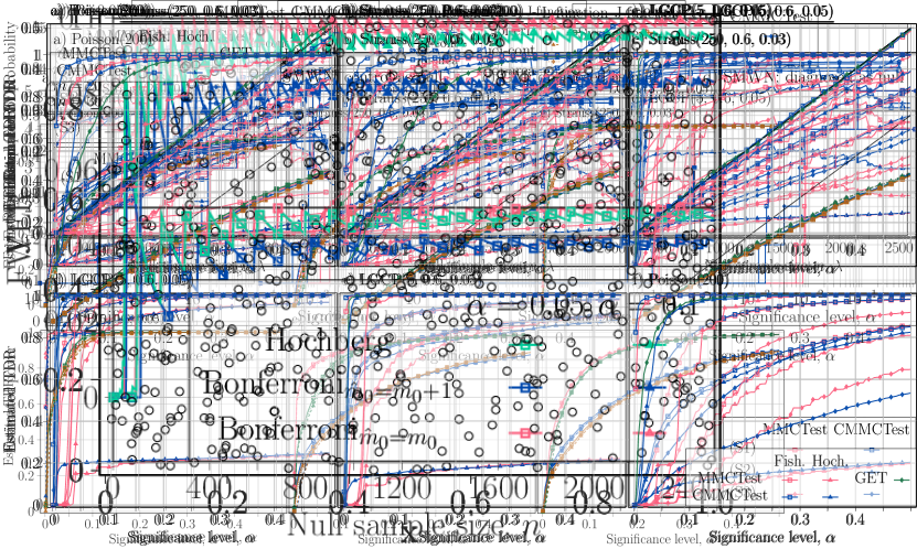
(b) ${\rm Poisson}(200)$

(c) ${\rm LGCP}(5,0.6,0.05)$

Figure 2: Example realizations of the point processes considered in the simulation study.

5.1 Power comparison: Storey’s BH procedure

Figure 3: Estimated power curves against the significance level, $\alpha$, when using Storey’s BH procedure with $\lambda=0.5$. At the top of the figure, the null distribution is underlined, while the non-true null distribution is read above each individual plot. All the plots share the same legend.

Figure 4: Estimated FDR curves against the significance level, $\alpha$, when using Storey’s BH procedure with $\lambda=0.5$. The black straight line, ${\rm FDR}=\alpha$, shows the nominal level. All the plots share the same legend.

We begin by comparing MMCTest to CMMCTest using power and FDR curves. In this simulation study, the centered L-function (Baddeley et al.) is used as the functional summary statistic, and the function ranking is done using the ERL measure in the R package GET (Myllymäki & Mrkvička (2024)), doing parallel ranking of the test point patterns, (7). We consider three cases:

1. known null distribution with $m_{0}=5$;

2. known null distribution with $m_{0}=9$;

3. unknown null distribution with $m_{0}=5$ and $10$ observations from the null.

In all these cases, we consider a simulation budget of $n=2500$, and $m=10$ test points. When fitting the models in Scenario (S3) we use maximum likelihood for Poisson, maximum profile pseudolikelihood for Strauss, and minimum contrast estimation with Ripley’s K-function for the log-Gaussian Cox process. This is done with default parameters using the standard model fitting functionality in spatstat (Baddeley et al. (2015)).

In Figure 3, where all the plots share the same legend, we show estimated power curves against the significance level, $\alpha$, when using Storey’s BH procedure with $\lambda=0.5$ for each of the $6$ combinations of null distributions and non-true null distributions and in the three scenarios (S1), (S2), and (S3). For the same cases, we show in Figure 4 the estimated FDR curves. We observe from Figure 3 that in nearly all cases CMMCTest dominates MMCTest in terms of power, with a few exceptions where the power is almost equal at relative large significance levels. Moreover, higher power is achieved when $m_{0}=5$ compared to when $m_{0}=9$, which is a standard consequence of multiplicity control: recall Storey’s BH procedure from Section 2.1 (Benjamini & Hochberg (1995); Storey et al. (2004)). Also, approximating the null distribution from only $10$ samples results in notable power loss in most cases, particularly in Figure 3a in which the null distribution is ${\rm Strauss}(250,0.6,0.03)$ and the non-true null distribution is ${\rm Poisson}(200)$. The power loss is substantial here since the considered Strauss and Poisson processes can yield quite similar point patterns, and in this specific numerical experiment, the estimate of the interaction parameter for one of the Strauss point patterns is one, thereby coinciding with Poisson. On the other hand, Figure 3e shows no loss in power due to approximating the null, which we attribute to the lack of importance of the exact value of the intensity in the L-function. Figure 4 shows that CMMCTest is conservative when using Storey’s BH procedure. This conservativeness is exacerbated when $m_{0}$ is smaller, and even more so when the null distribution must be approximated.

Figure 5: Estimated FDR according to the choice of Storey’s parameter, $\lambda$. All the plots share the same legend.

The preceding numerical experiments raises a question regarding the choice of the $\lambda$ hyperparameter used in Storey’s estimator, cf. Definition 3. We have explored the influence of this choice for the same scenarios as previous for $\alpha=0.05$. We see in Figure 5 that Storey’s BH procedure is not sensitive to the choice of the parameter $\lambda$, and that the procedure is conservative for any $\lambda\in(0,1)$ as suggested by Theorem 3. Particularly, it seems that choosing $\lambda\in[0.1,0.7]$ yields comparable FDR. We skip showing the corresponding power curves as they output the same conclusions.

5.2 Choice of conformal score

So far we have only considered one type of conformal score in using the ERL measure for the centered L-function doing the ranking in parallel for each of the test point patterns. We consider now different GET measures, specifically the continuous rank measure, denoted cont, and the area measure, denoted area, both proposed by Mrkvička et al. (2022). Moreover, we use also the J-function (see van Lieshout & Baddeley (1996)) in place of the centered L-function. Finally, we try also the joint ranking of (6).

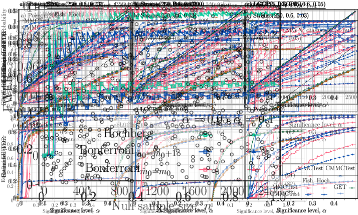
Figure 6: Estimated power curves against the significance level, $\alpha$, when using Storey’s BH procedure with $\lambda=0.5$ for a variety of conformal scores. At the top of the figure, the null distribution is underlined, while the non-true null distribution is read above each individual plot.

Figure 7: Estimated FDR curves against the significance level, $\alpha$, when using Storey’s BH procedure with $\lambda=0.5$ for a variety of conformal scores. The black straight line, ${\rm FDR}=\alpha$, shows the nominal level.

We use Storey’s BH procedure with $\lambda=0.5$, $n=2500$, and consider $m=10$ with $m_{0}=5$. Figure 6 shows the TDR for all the test cases, while the corresponding FDR is found in Figure 7. We observe in Figure 6 that no substantial differences occur whether we use the ERL measure, the cont measure, or the area measure. Moreover, we notice that the centered L-function tends to yield a more powerful test than that of the J-function, which is consistent with the observations of Mrkvička et al. (2017).

Finally, we see that doing parallel ranking of the test point patterns in all cases yields a uniformly more powerful test than doing joint ranking. This is due to an additional dependency added in the $p$-values when doing the joint ranking. Hence, there is a trade-off between computational complexity and performance: if the cost of doing the functional ranking is not substantial, the parallel ranking is preferred, however, in cases where $m$ is very large so the computational demands of doing the parallel ranking is impractical, the joint ranking can be used. We remark also that in most cases, using the CMMCTest with the joint ranking is still more powerful than MMCTest, which can be seen by comparing Figure 6 and Figure 3.

5.3 Robustness against multiplicity

In this scenario, we consider different settings of triplets $(\alpha,m,n)$. This has been studied theoretically by Mary & Roquain (2022) and Marandon et al. (2024), while in the current study we evaluate numerically the power through simulations and focus on the benefit of using the CMMCTest as compared to MMCTest. The null distribution is ${\rm Poisson}(200)$ and the non-true null distribution is ${\rm Strauss}(250,0.6,0.03)$, setting $m_{0}=m/2$ in all cases, and we use Storey’s BH procedure with $\lambda=0.5$. In Figure 8, we show the TDR for $\{(\alpha,m,n):\alpha\in\{0.05,0.1,0.2\},m\in\{6,10,20,30\},n\subset\{240,\dots,2520\}\}$. We observe that for CMMCTest, the value of $m$ has little influence, and when $\alpha=0.2$ having a larger $m$ can even give slight improvements in TDR. Meanwhile, a large $m$ is detrimental to the power of MMCTest, and only the case $\alpha=0.2$ with $m\in\{6,10\}$ shows comparable performance to the CMMCTest.

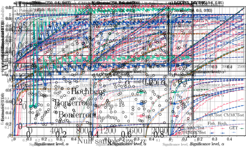
Figure 8: Estimated TDR of the MMCTest and CMMCTest for varying triplets $(\alpha,m,n)$. All the plots share the same legend.

5.4 Power comparison: Hochberg procedure

As shown in Theorem Conjecture, using the Hochberg procedure we can control the FWER with conformal $p$-values. We report here results using the Hochberg procedure for scenarios (S1), (S2), and (S3): TDR curves are shown in Figure 9, and FWER curves are shown in Figure 10. Firstly, we see from Figure 10 that indeed we control the FWER, and that estimating the null model, or having a larger $m_{0}$, results in a more conservative test. Inspecting Figure 9 and comparing to Figure 3 we notice that for $m=10$ with $m_{0}=5$ the power loss of the Hochberg procedure in comparison to Storey’s BH procedure is not so pronounced, however, when $m_{0}=9$ the strict FWER criterion leads to a severe loss in power. In all cases, estimating the null model results in a loss in power as expected and also seen previously for Storey’s BH procedure. Finally, we note once again that the CMMCTest outperforms the MMCTest in nearly all considered cases.

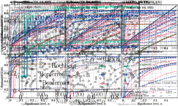
Figure 9: Estimated power curves against the significance level, $\alpha$, when using the Hochberg procedure. At the top of the figure, the null distribution is underlined, while the non-true null distribution is read above each individual plot. All the plots share the same legend.

Figure 10: Estimated FWER curves against the significance level, $\alpha$, when using the Hochberg procedure. The black straight line, ${\rm FWER}=\alpha$, shows the nominal level. All the plots share the same legend.

6 Real data set: Sweat glands

The sweat gland data considered in Kuronen et al. (2021) includes three groups of point patterns, see Figure 11: (i) a control group of $4$ subjects (numbers 96, 149, 203, 205) (ii) a group of $5$ subjects (numbers 10, 20, 40, 61, 71) suspected to have neuropathy (MNA), and (iii) a group of $5$ subjects (numbers 23, 36, 42, 50, 73) diagnosed with MNA. For the point pattern data, three different models were proposed: (i) a sequential point process model, (ii) a sequential point process model with noise (SMWN), and (iii) a generative model (GM). For each model, a parameter estimation method was proposed, which for the sequential point process models was based on maximum likelihood and for the generative model relied on approximate Bayesian computation Markov chain Monte Carlo sampling since for this model the likelihood is intractable.

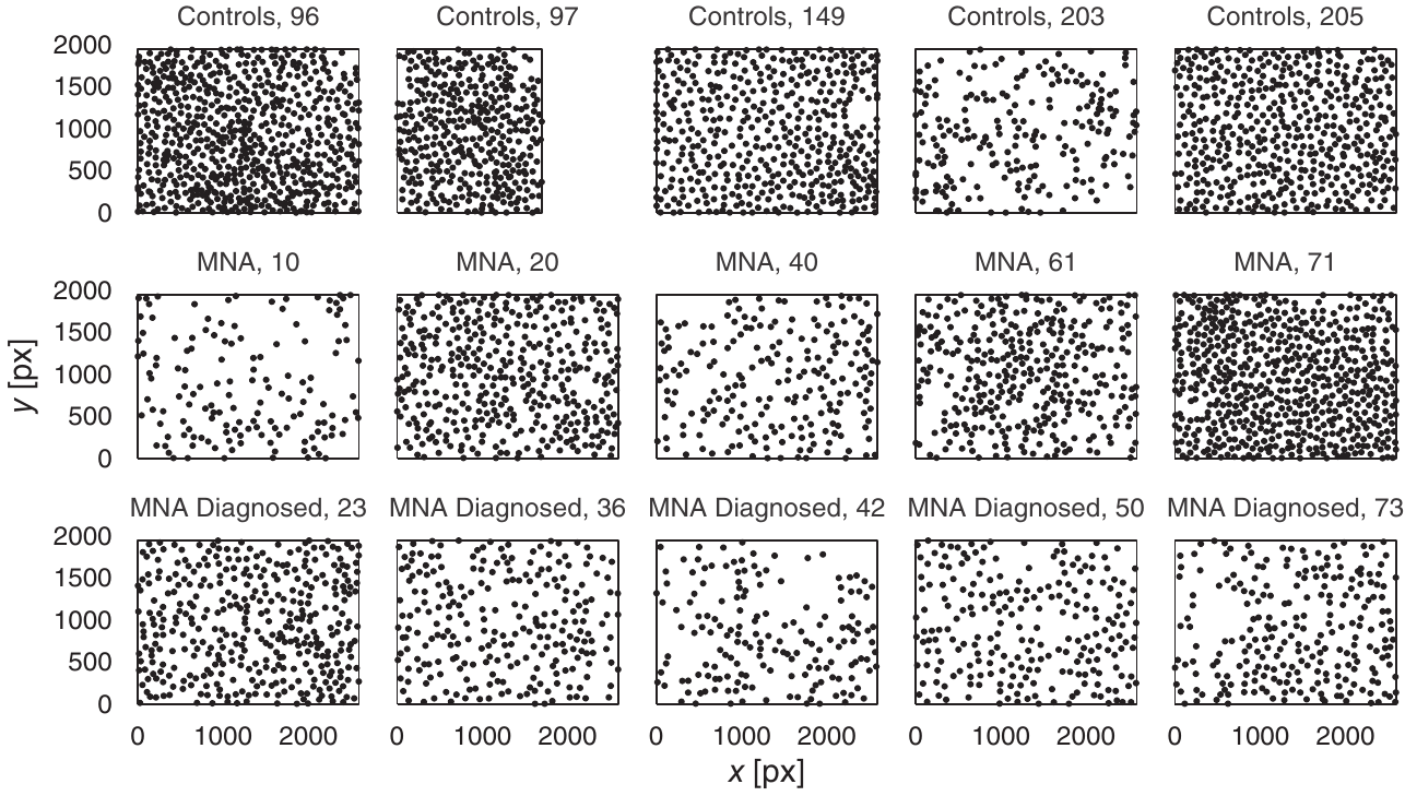
Figure 11: The sweat gland data. Figure taken from Kuronen et al. (2021).

With this data different null hypotheses can be considered. Firstly, one could consider the null hypothesis that a subject does not have MNA. In this case, the control group should be considered as the null sample, and we can run a multiple testing procedure on the MNA suspected and MNA diagnosed groups. Secondly, one could consider the null hypothesis that a subject has MNA. In this case, the MNA diagnosed group should be considered as the null sample, and we can run a multiple testing procedure on the MNA suspected and control groups. For both of these null hypotheses, we could use any (or all) of the proposed models and associated inference algorithms proposed in Kuronen et al. (2021) in order to increase the size of the null sample, as $5$ is not sufficient.

Figure 12 shows the number of rejections in the four cases considering either the MNA diagnosed subjects as the null sample or the control subjects as the null sample, and using either the sequential model with noise or the generative model as the parametric model, discussed in Section 4.2, to simulate point patterns. In all cases, Storey’s BH procedure is used with $\lambda=0.5$ and simulating $n=5000$ point patterns under the fitted null distributions.

Figure 12: Number of rejections against the significance level, $\alpha$.

We observe from Fig 12, that using the sequential model with noise generally leads to more rejections than for the generative model. Firstly, this indicates that the sequential model with noise yields a better and more representative fit on the null sample than the generative model. Secondly, it reveals a profound weakness of the parametric data augmentation in that different hypothesized models can result in very different conclusions made from the test. We also observe more rejections of the control subjects than the MNA suspected subjects when using the MNA diagnosed subjects as the null sample, which is desirable. Moreover, we observe more rejections when using CMMCTest compared to MMCTest in almost all cases, indicating the power improvements we expect from the CMMCTest.

In Figure 13 we show the global envelopes which gives a graphical interpretation, as discussed in Section 4.2, when using the sequential model with noise with the control subjects as the null sample. We use Storey’s BH procedure with $\lambda=0.5$ at level $\alpha=0.05$, the centered L-function, and the parallel ERL measure. The observed summary statistics are compared to the upper and lower envelopes with red dots indicating that the observation is more extreme than the null sample at the nominal level. Storey’s estimate yields $\hat{m}_{0}=2$.

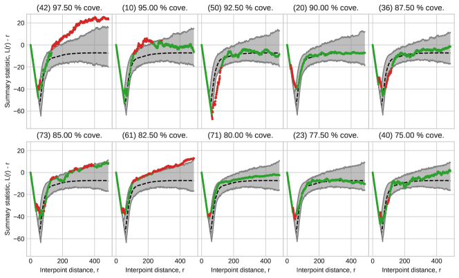
Figure 13: Graphical interpretation of rejection decisions for the sequential model with noise with control as null.

Figure 13 shows that all the point patterns are rejected meaning that all the MNA suspected and diagnosed subjects are statistically significantly different from the control subjects, consistent with Figure 12. The interesting part here is that we can interpret the reason for rejection: for all the point patterns (except subject 10) the summary statistic falls outside of the envelope at small values of $r$, while further some of the point patterns (including subjects 42, 10, and 61) breaks the upper envelope at higher values of $r$. This gives the interpretation that to make the rejection decision, we are exploiting the properties that the L-functions of the control subjects have a lower variability on the level of repulsion at small $r$, while tending to have repulsive/less clustered behavior at larger $r$.

7 Conclusion

We proposed conformal multiple Monte Carlo testing (CMMCTest), a framework for multiple Monte Carlo testing using recent developments on conformal novelty detection. CMMCTest efficiently re-uses the null sample, cutting computational costs while maintaining rigorous control over FDR or FWER. We highlight the connection between conformal novelty detection and Barnard’s Monte Carlo test, and investigate its use within the area of spatial statistics. Here functional ranking measures can be used to construct conformal scores yielding powerful multiple testing procedures. Simulations and a real-world application to sweat gland data showed CMMCTest’s superior statistical power within a fixed computational budget.

Directions for future work include exploring the existence of more powerful multiple testing procedures controlling the FWER with conformal p-values and non-parametric data augmentation techniques to avoid the problems with the parametric method.

8 Acknowledgments

The authors extend their gratitude to Ottmar Cronie and Etienne Roquain for fruitful discussions and give thanks to Aila Särkkä for discussions surrounding real data applications.

Online Supplementary Material for ”Conformal novelty detection for replicate point patterns with FDR or FWER control”

Christophe A. N. Biscio
Department of Mathematical Sciences, Aalborg University
and
Adrien Mazoyer
Institut de Mathématiques de Toulouse, UMR5219 CNRS
and
Martin V. Vejling
Department of Mathematical Sciences, Aalborg University

Appendix A On the distribution of ordered conformal p-values

We present in this section some new results regarding the joint distribution of the order statistics of the conformal p-values. First, we find the joint probability mass function.

Lemma 1.

Let assumptions ($\mathcal{A}$1)-($\mathcal{A}$3) be true for a conformal score $\hat{s}$, and consider $m$ test points $\boldsymbol{X}_{n+1},\dots,\boldsymbol{X}_{n+m}$ such that $(\boldsymbol{X}_{n+i})_{i\in\mathcal{H}_{0}}$ are jointly independent of each other. Then, the joint probability mass function of the order statistics of the $p$-values, denoted $\hat{\boldsymbol{p}}_{()}=[\hat{p}_{(1)},\dots,\hat{p}_{(m)}]^{\top}$, is

$$\mathbb{P}(\hat{\boldsymbol{p}}_{()}=\boldsymbol{j}/(n+1))=\mathbbm{1}[j_{1}\leq\cdots\leq j_{m}]\frac{n!m!}{(n+m)!},$$ (8)

for $\boldsymbol{j}=[j_{1},\dots,j_{m}]^{\top}$, i.e., the discrete uniform distribution on the integer order set

$$\{(x_{1},\dots,x_{m}):x_{1}\leq\cdots\leq x_{m},x_{j}\in\{1/(n+1),\dots,1\},j=1,\dots,m\}.$$

Proof.

We know the joint probability mass function, see (2), and notice that the joint probability mass function is invariant to permutations. This is exploited to find the joint distribution of the order statistics. Specifically, Song2024:Order Theorem 2.1.2 gives that

$$\mathbb{P}(\hat{\boldsymbol{p}}_{()}=\boldsymbol{j}/(n+1))=\frac{\mathbbm{1}[j_{1}\leq\cdots\leq j_{m}]}{{\prod_{k=1}^{n+1}M_{k}(\boldsymbol{j})!}}\displaystyle\sum_{\boldsymbol{i}\in\mathcal{A}^{m}}\mathbb{P}\bigg{(}\bigcap_{k=1}^{m}\hat{p}_{i_{k}}=\frac{j_{k}}{n+1}\bigg{)},$$

where $\mathcal{A}^{m}$ is the set of arrangements of $\{1,\dots,m\}$. Noticing that the joint probability mass function is invariant to permutations, the sum can be replaced by a multiplication of $|\mathcal{A}^{m}|=m!$. Inserting the joint probability mass function, see (2), yields (8). ∎

Below is a technical lemma which will be required later.

Lemma 2.

For $n\geq 1$ and $m\geq 0$ the following identity holds

$$\sum_{y=1}^{n}\frac{(y+m-1)!}{(y-1)!}=\frac{(n+m)!}{(m+1)(n-1)!}.$$

Proof.

Dividing by $m!$ on the left hand side yields

$$\sum_{y=1}^{n}\frac{(y+m-1)!}{(y-1)!m!}=\sum_{y=1}^{n}\binom{y-1+m}{m}=\binom{n+m}{m+1}=\frac{1}{m!}\frac{(n+m)!}{(m+1)(n-1)!}$$

where the second equality is the Hockey Stick Identity, see Jones1996Supp:Hockey. ∎

Equipped with the joint distribution, we can also derive the marginals.

Corollary 1.

Let assumptions ($\mathcal{A}$1)-($\mathcal{A}$3) be true for a conformal score $\hat{s}$, and consider $m$ test points $\boldsymbol{X}_{n+1},\dots,\boldsymbol{X}_{n+m}$ such that $(\boldsymbol{X}_{n+i})_{i\in\mathcal{H}_{0}}$ are jointly independent of each other. Then, the marginal probability mass function of the $i$-th smallest p-value is

$$\mathbb{P}(\hat{p}_{(i)}=j/(n+1))=\frac{n!m!}{(n+m)!}\frac{(j+i-1)!}{(j-1)!(i-1)!}\frac{(n+m-j-i+2)!}{(n-j+1)!(m-i)!}.$$

Proof.

We compute directly the marginal by summing over the joint:

$$\mathbb{P}(\hat{p}_{(i)}=j/(n+1))=\frac{n!m!}{(n+m)!}\bigg{(}\sum_{y_{i-1}=1}^{j}\cdots\sum_{y_{2}=1}^{y_{3}}\sum_{y_{1}=1}^{y_{2}}1\bigg{)}\bigg{(}\sum_{y_{m}=j}^{n+1}\cdots\sum_{y_{i+2}=j}^{y_{i+3}}\sum_{y_{i+1}=j}^{y_{i+2}}1\bigg{)}.$$

The result follows immediately by evaluating the sums. Specifically, computing the first sums

$$\sum_{y_{i-1}=1}^{j}\cdots\sum_{y_{2}=1}^{y_{3}}\sum_{y_{1}=1}^{y_{2}}1=\sum_{y_{i-1}=1}^{j}\cdots\sum_{y_{2}=1}^{y_{3}}y_{2}=\sum_{y_{i-1}=1}^{j}\cdots\sum_{y_{2}=1}^{y_{3}}\frac{y_{2}!}{(y_{2}-1)!}.$$

Applying Lemma 2 repeatedly gives

$$\sum_{y_{i-1}=1}^{j}\cdots\sum_{y_{2}=1}^{y_{3}}\sum_{y_{1}=1}^{y_{2}}1=\sum_{y_{i-1}=1}^{j}\cdots\sum_{y_{3}=1}^{y_{4}}\frac{(y_{3}+1)!}{2(y_{3}-1)!}=\frac{(j+i-1)!}{(j-1)!(i-1)!}.$$

The other sums are evaluated by the same arguments. ∎

Unfortunately, working with the marginals will not be sufficient in the following.

Given the explicit joint probability mass function, we present here a direct proof, which is arguably simpler than that of Angelopoulos2024Supp:Theoretical, that the Bonferroni-type procedure rejecting at level $1-(1-\alpha)^{1/m}$ controls the FWER at level $\alpha$.

Theorem 4.

Let assumptions ($\mathcal{A}$1)-($\mathcal{A}$3) be true for a conformal score $\hat{s}$, and consider $m$ test points $\boldsymbol{X}_{n+1},\dots,\boldsymbol{X}_{n+m}$ such that $(\boldsymbol{X}_{n+i})_{i\in\mathcal{H}_{0}}$ are jointly independent of each other. Then, the conformal $p$-values satisfies

$$\mathbb{P}\left(\bigcup_{j=1}^{m}\left\{\hat{p}_{j}\leq 1-(1-\alpha)^{1/m}\right\}\right)\leq\alpha.$$

Additionally, as $n\to\infty$, $\mathbb{P}\left(\bigcup_{j=1}^{m}\left\{\hat{p}_{j}\leq 1-(1-\alpha)^{1/m}\right\}\right)=\alpha$.

Proof.

From Lemma 1, the joint probability mass function of the ordered conformal $p$-values is

$$\mathbb{P}(\hat{\boldsymbol{p}}_{()}=\boldsymbol{j}/(n+1))=\mathbbm{1}[j_{1}\leq\cdots\leq j_{m}]\frac{n!m!}{(n+m)!}.$$

We have that ${\rm FWER}=\mathbb{P}\big{(}\bigcup_{j=1}^{m}\hat{p}_{j}\leq 1-(1-\alpha)^{1/m}\big{)}=1-\mathbb{P}\big{(}\bigcap_{j=1}^{m}\hat{p}_{(j)}>1-(1-\alpha)^{1/m}\big{)}$. Let $t=\lfloor(1-(1-\alpha)^{1/m})(n+1)\rfloor$ denote the $p$-values threshold, and compute the FWER:

$${\rm FWER}=1-\frac{n!m!}{(n+m)!}\sum_{y_{m}=t+1}^{n+1}\sum_{y_{m-1}=t+1}^{y_{m}}\cdots\sum_{y_{1}=t+1}^{y_{2}}1=1-\frac{n!}{(n+m)!}\prod_{k=0}^{m-1}(n+1-t+k)$$

which follows from the same arguments as in the proof of Corollary 1. Then, by inserting the expression for $t$

$${\rm FWER} =1-\frac{n!}{(n+m)!}\prod_{k=0}^{m-1}(n+1-\lfloor(1-(1-\alpha)^{1/m})(n+1)\rfloor+k)$$

$$\leq 1-\frac{n!}{(n+m)!}\prod_{k=0}^{m-1}((1-\alpha)^{1/m}(n+1)+k)$$

$$\leq 1-\frac{n!}{(n+m)!}(1-\alpha)\prod_{k=0}^{m-1}(n+1+k)=\alpha.$$

The errors made in the inequalities goes to zero as $n\to\infty$, concluding the proof. ∎

As mentioned in the paper, if the $p$-values are ${\rm MTP}_{2}$, then the Hochberg procedure controls the FWER. We will show now that the conformal $p$-values indeed are not ${\rm MTP}_{2}$, but first we define the notion of ${\rm MTP}_{2}$.

Definition 6 (${\rm MTP}_{2}$ (Benjamini2001Supp:Dependency)).

A random vector $\boldsymbol{X}$ is ${\rm MTP}_{2}$ if for all $\boldsymbol{x}$, $\boldsymbol{y}$ we have

$$f(\boldsymbol{x})f(\boldsymbol{y})\leq f({\rm min}(\boldsymbol{x},\boldsymbol{y}))f({\rm max}(\boldsymbol{x},\boldsymbol{y}))$$

where the minimum and maximum is component wise and $f$ is either the joint density or the joint probability distribution of $\boldsymbol{X}$.

Theorem 5.

Let assumptions ($\mathcal{A}$1)-($\mathcal{A}$3) be true for a conformal score $\hat{s}$, and consider $m$ test points $\boldsymbol{X}_{n+1},\dots,\boldsymbol{X}_{n+m}$ such that $(\boldsymbol{X}_{n+i})_{i\in\mathcal{H}_{0}}$ are jointly independent of each other. Then, the conformal $p$-values are not ${\rm MTP}_{2}$.

Proof.

We know the joint probability mass function, see (2). As a counter example, consider a case where $n=2$ and $m=3$, and let $\boldsymbol{x}=[2/3,2/3,2/3]^{\top}$ and $\boldsymbol{y}=[1/3,1,1/3]^{\top}$. Then $f(\boldsymbol{x})=6$ and $f(\boldsymbol{y})=2$, while $f({\rm min}(\boldsymbol{x},\boldsymbol{y}))=2$ and $f({\rm max}(\boldsymbol{x},\boldsymbol{y}))=2$, showing that $f(\boldsymbol{x})f(\boldsymbol{y})>f({\rm min}(\boldsymbol{x},\boldsymbol{y}))f({\rm max}(\boldsymbol{x},\boldsymbol{y}))$ in this case, and thereby disproving the ${\rm MTP}_{2}$ property. ∎

We are also interested in expressing the joint survival function of the ordered conformal $p$-values, when a sequence of thresholds $t_{1}\leq t_{2}\leq\cdots\leq t_{m}$ is used. To do so, requires summing over the joint probability mass function which amounts to counting grid points on a discrete order set.

Lemma 3.

Given $t_{1}\leq\dots\leq t_{m}\in\{0,\dots,n\}$, let $P_{m-1}[y]=\sum_{i=0}^{m-1}a_{i}^{(m-1)}y^{i}$, $y\in\mathbb{N}$, be $(m-1)$-th order polynomials, defined recursively as $P_{m}[x]=\sum_{y=t_{m}+1}^{x}P_{m-1}[y]$ with initial conditions $P_{0}[y]=1$. Then, $P_{m}[n+1]$ is the number of grid points on (cardinality of) the discrete order set $\{(x_{1},\dots,x_{m}):x_{1}\leq\cdots\leq x_{m},x_{j}\in\{(t_{j}+1)/(n+1),\dots,1\},j=1,\dots,m\}$. Moreover, the polynomial coefficients are defined recursively as

$$a_{0}^{(m)} =-\sum_{j=0}^{m-1}\frac{a_{j}^{(m-1)}}{j+1}\sum_{r=0}^{j}\binom{j+1}{r}B_{r}t_{m}^{j+1-r},$$ (9)

$$a_{i}^{(m)} =\sum_{j=i-1}^{m-1}\frac{a_{j}^{(m-1)}}{j+1}\binom{j+1}{i}B_{j+1-i},\quad 0<i\leq m,$$ (10)

where $B_{r}$ is the $r$-th Bernoulli number (see Apostol2008Supp:Bernoulli) with the convention $B_{1}=1/2$.

Proof.

Consider the sum $P_{m}[n+1]=\sum_{y_{m}=t_{m}+1}^{n+1}\sum_{y_{m-1}=t_{m-1}+1}^{y_{m}}\cdots\sum_{y_{1}=t_{1}+1}^{y_{2}}1$, which is the sum over the discrete order set. Initially, we have $P_{0}[y_{1}]=1$, followed by $P_{1}[y_{2}]=\sum_{y_{1}=t_{1}+1}^{y_{2}}1=y_{2}-t_{1}$. Faulhaber’s formula (for a brief primer see Larson2019Supp:Bernoulli) states that

$$\sum_{k=1}^{n}k^{p}=\frac{1}{p+1}\sum_{r=0}^{p}\binom{p+1}{r}B_{r}n^{p+1-r},$$

meaning that the sum over a polynomial of order $m-1$ is a polynomial of order $m$. By an inclusion-exclusion argument $\sum_{k=t+1}^{n}k^{p}=\sum_{k=1}^{n}k^{p}-\sum_{k=1}^{t}k^{p}$ we can handle the varying starting points of the sums. Now, by the recursive definition

$$P_{m}[n+1] =\sum_{i=0}^{m-1}\Big{(}\sum_{y=1}^{n+1}a_{i}^{(m-1)}y^{i}-\sum_{y=1}^{t_{m}}a_{i}^{(m-1)}y^{i}\Big{)}$$

$$=\sum_{i=0}^{m-1}\frac{a_{i}^{(m-1)}}{i+1}\sum_{r=0}^{i}\binom{i+1}{r}B_{r}\Big{(}(n+1)^{i+1-r}-t_{m}^{i+1-r}\Big{)}.$$

Collecting the terms yields the formulas in (9)-(10). ∎

This result motivates an algorithm for computing the number of grid points on the discrete order set which is only of $O(m^{3})$, a drastic improvement on a naïve approach which is $O(n^{m})$. In turn, this allows us to efficiently compute the joint survival function $\mathbb{P}\big{(}\bigcap_{j=1}^{m}\hat{p}_{(j)}>t_{j}/(n+1)\big{)}=\frac{n!m!}{(n+m)!}P_{m}[n+1]$, and then applying De Morgan’s laws ${\rm FWER}=1-\frac{n!m!}{(n+m)!}P_{m}[n+1]$, meaning that for a given sequence of thresholds $t_{j}$, $j=1,\dots,m$, we can compute exactly the ${\rm FWER}$. Notably, for the Hochberg procedure, $t_{j}=\lfloor\frac{\alpha}{m-j+1}(n+1)\rfloor$, while for the sharp Bonferroni procedure it is $t_{j}=\lfloor(1-(1-\alpha)^{1/m})(n+1)\rfloor$. When $m>m_{0}$, the Bonferroni procedure can be further sharpened by first estimating $\hat{m}_{0}$ with a liberal estimate (for instance Storey’s estimate), and then using $t_{j}=\lfloor(1-(1-\alpha)^{1/\hat{m}_{0}})(n+1)\rfloor$.

Finally, we proof for $m\in\{1,2,3,4,5\}$, the statement which we conjectured for general $m$ in Corollary Conjecture.

Theorem 6.

Let assumptions ($\mathcal{A}$1)-($\mathcal{A}$3) be true for a conformal score $\hat{s}$. Then, for $m\in\{1,2,3,4,5\}$, the Hochberg procedure (See Definition 4) at level $\alpha$ with the conformal $p$-values satisfies

$${\rm FWER}=\mathbb{P}(V\geq 1)\leq\alpha.$$

Proof.

The case $m=1$ follows immediately from the superuniformity of the conformal $p$-values. For the cases $m>1$, the proof can be made by evaluating $\frac{m!}{(n+1)_{m}}P_{m}[n+1]$ and arguing that this is greater than or equal to $1-\alpha$. We skip the computations for the cases $m=2,3,4$, remarking that the case $m=2$ is relatively simple, however from $m=3$ and onward, the proof contains lengthy calculus. We report in the following the case $m=5$, where lengthy calculus is done using computer assistance.

Let $k\lfloor\alpha(n+1)\rfloor\leq\alpha(n+1)$ such that $k/(n+1)\leq\alpha$. Note then that $t_{m}=k$ and $t_{m-i}=\lfloor\frac{\alpha}{(i+1)}(n+1)\rfloor=\lfloor\frac{\lfloor\alpha(n+1)\rfloor}{(i+1)}\rfloor=\lfloor\frac{k}{(i+1)}\rfloor\leq\frac{k}{(i+1)}$. From this it follows that

$$P_{m}[n+1]\geq\sum_{y_{m}=k+1}^{n+1}\sum_{y_{m-1}=k/2+1}^{y_{m}}\cdots\sum_{y_{1}=k/m+1}^{y_{2}}1.$$ (11)

Now, doing the evaluations for the case $m=5$ we get

$$\begin{split}\frac{120}{(n+1)_{5}}P_{5}[n+1]&\geq\frac{120(n+1-k)}{(n+1)_{5}}\bigg{(}\frac{(n+2)_{4}}{120}+\frac{243k^{4}}{103680}+\frac{k^{3}(256n+2942)}{103680}\\ &\qquad\qquad+\frac{36k^{2}(9n^{2}+109n+398)}{103680}+\frac{144k(9n^{2}+77n+172)}{103680}\bigg{)}\end{split}$$

$$>\frac{120(n+1-k)}{(n+1)_{5}}\frac{(n+2)_{4}}{120}=1-\frac{k}{n+1}\geq 1-\alpha,$$

where $(x)_{k}=(x+k-1)!/(x-1)!$, for $x,k\geq 1$, is the rising factorial, and where the first inequality follows from (11), the second inequality holds since the excluded terms are all positive, and the third inequality is due to the definition of $k$. ∎

The preceding theorem and proof only verifies the Hochberg procedure until $m=5$, however, this in no way implies that the statement is false for larger $m$. On the contrary, we conjecture that the same arguments could be applied for larger $m$, although a proof for general $m$ has eluded us.

Appendix B Testing a global null hypothesis

Here we consider testing the global null hypothesis $H_{0}:P_{j}=P_{0}$, for all $j=1,\dots,m$. In this case, we make no assertions regarding individual point patterns and instead test for group effects. We are interested in controlling the type I error probability at a specified significance level $\alpha\in(0,1)$. This is the multiple testing scenario of Mrkvicka2017Supp:Multiple where global envelope tests are used with the concatenated functional summary statistics of the test points. Specifically, let $T_{1},\dots,T_{m}$ denote the functional summary statistics of the test data, then the functions are concatenated as $T=[T_{1},\dots,T_{m}]^{\top}$, and a global envelope test is made considering $T$ to be the functional summary statistic of the test data. This procedure controls the type I error probability at the nominal level.

Figure 14: Estimated power curves against the significance level, $\alpha$, when testing a global null hypothesis. At the top of the figure, the null distribution is underlined, while the non-true null distribution is read above each individual plot. All the plots share the same legend. Fish. and Hoch. are shorthand for Fisher combination test and Hochberg procedure, respectively.

In light of the methodology proposed in this work, other approaches can be taken. An immediate idea is to run the Hochberg procedure on either the MMCTest $p$-values or the CMMCTest $p$-values and rejecting the global null $H_{0}$ if one or more of the local null hypotheses are rejected. A more powerful method might be to use a combination test, for instance a Fisher combination test Fisher1925Supp:Statistical. The Fisher combination test works for the independent $p$-values of the MMCTest. Theorem 2.2 of Bates2023Supp:Testing shows that a corrected Fisher combination test controls the type I error probability when using conformal $p$-values, which we expect to be a very powerful method considering the power gains observed so far with the CMMCTest compared to the MMCTest.

We make a simulation study with the point processes as in Section 5 with the scenario (S1), and show power curves in Figure 14 and type I error probability curves in Figure 15. We observe significant power gains compared to the multiple GET method of Mrkvicka2017Supp:Multiple, particularly the most powerful procedure is the corrected Fisher combination test on the conformal $p$-values in all the test cases.

Figure 15: Estimated type I error probability curves against the significance level, $\alpha$, when testing a global null hypothesis. The black straight line shows the nominal level. All the plots share the same legend. Fish. and Hoch. are shorthand for Fisher combination test and Hochberg procedure, respectively.

agsm mybib.bib