Machine Learning Fairness for Depression Detection using EEG Data

Abstract

This paper presents the very first attempt to evaluate machine learning fairness for depression detection using electroencephalogram (EEG) data. We conduct experiments using different deep learning architectures such as Convolutional Neural Networks (CNN), Long Short-Term Memory (LSTM) networks, and Gated Recurrent Unit (GRU) networks across three EEG datasets: Mumtaz, MODMA and Rest. We employ five different bias mitigation strategies at the pre-, in- and post-processing stages and evaluate their effectiveness. Our experimental results show that bias exists in existing EEG datasets and algorithms for depression detection, and different bias mitigation methods address bias at different levels across different fairness measures.

Index Terms—  EEG, ML fairness, Depression Detection

1 Introduction

Major depressive disorders (MDD) are becoming increasingly prevalent worldwide. Machine learning (ML), especially deep learning (DL) based methods, have been recently used in many research studies for depression detection with success [1, 2, 3]. In concurrence, ML bias is becoming a growing source of concern [4]. Bias can be understood as discrimination against individuals based on certain sensitive attributes such as age, race and gender [5, 6, 7]. Fairness conversely dictates that no individual or subgroup should be advantaged or disadvantaged based on their inherent characteristics. Given the high stakes involved in MHD analysis, it is crucial to investigate and mitigate the ML biases present. Research indicated the presence of ML bias across a variety of tasks ranging from automated video interviews [8] to image search [9]. However, none of the existing works have addressed ML fairness in MDD detection using EEG data.

Our contributions in this paper are as follows. First, our study is the first attempt to evaluate ML fairness for depression detection using electroencephalogram (EEG) data. None of the existing work on ML fairness for depression detection [10, 11, 12, 13] has investigated bias mitigation for depression detection using EEG data. Second, we study and compare the effectiveness of a diverse set of bias mitigation techniques to improve fairness in EEG-based depression detection. We show they have different effects on performance and fairness. We conduct our experiments using three different deep architectures across three datasets, Mumtaz, MODMA and Rest. Throughout our experimentation, we attempt to address the following two research questions (RQs). RQ 1: Is there bias within existing EEG data and ML algorithm for depression detection? RQ 2: How effective are existing bias mitigation methods at improving ML fairness for depression detection using EEG data? Our experimental results indicate that both data and algorithmic biases exist and that different bias mitigation provides different degree of effectiveness across different datasets and algorithms.

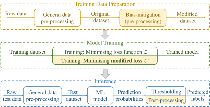
Fig. 1: Simplified pipeline: highlighted parts indicate how bias is mitigated at the pre-, in- and post-processing stages.

2 Methodology

We approach MDD detection as a classification problem where we have a dataset $D=\{(\mathbf{x}_{i},y_{i})\}_{i}$ where $\mathbf{x}_{i}\in X$ is a tensor representing information (e.g. EEG data) about an individual $I$ and $y_{i}\in Y$ is the outcome (e.g. 1 for depressed vs. 0 for non-depressed) that we wish to predict. Each input $\mathbf{x}_{i}$ is associated (through an individual $I$) with a sensitive attribute $s(\mathbf{x}_{i})\in S$ where $S=\{male,female\}$. This is a classification problem where we are interested in finding a parameterised function $f$ with $f:X\rightarrow Y$. $f(\ \cdot\ ;\theta)$ estimates the probabilities for all outcomes (classes) $p(Y|\mathbf{x}_{i})$. We use $p(y_{i}|\mathbf{x}_{i})$ to denote the predicted probability for the correct class. The goal of bias mitigation is to ensure that the outcomes for each demographic subgroup adhere to the different fairness measures outlined in Section 2.2.

2.1 Bias Mitigation Methods

We employ two pre-processing, two in-processing and one post-processing bias mitigation methods. Each method has its own advantages and disadvantages. Pre- and post-processing may be easier to implement but in-processing may be the most effective [4]. We have chosen the commonly used methods according to [5].

(a) Pre-processing: Data Augmentation

We employ a data augmentation technique, Mixup [14], which works by generating new samples for the minority group so that the resulting dataset is balanced across gender. A new sample $(\mathbf{x}^{\prime},y^{\prime})$ is generated from two randomly drawn examples $(\mathbf{x}_{i},y_{i})$ and $(\mathbf{x}_{j},y_{j})$ with $i\neq j$ via:

$$\footnotesize\mathbf{x}^{\prime}=\lambda\mathbf{x}_{i}+(1-\lambda)\mathbf{x}_{j},$$ (1)

$$y^{\prime}=\lambda y_{i}+(1-\lambda)y_{j},$$ (2)

where $\lambda\sim\mathrm{Beta}(\alpha)$ for some hyperparameter $\alpha$ that controls the strength of interpolation. We use $\alpha=0.4$ as it gives the best results within our experiments.

(b) Pre-processing: Massaging

We implement massaging proposed by Kamiran and Calders [15] by producing a modified dataset by relabelling the same number of instances from the favoured community with a favourable label and instances from the deprived community with an unfavourable label. For a dataset $D$, the favoured community ($s_{\mathrm{fav}}$) refers to the demographic group with a higher probability of belonging to the favourable class $y_{+}$, and the other group is called the deprived community ($s_{\mathrm{dep}}$). Since we are interested in detecting depression, $y_{+}$ refers to the depressed class. After relabelling, the distribution of classes is unchanged, but the class distribution is now the same across both genders, and the gender ratio is equal in both classes.

(c) In-processing: Reweighing

We implemented reweighing which calculates weights $\beta_{i}$ for each example. We then modify the original loss function (e.g., Cross-Entropy Loss) for a batch $B$:

$$\footnotesize\mathcal{L}(B)=\frac{1}{|B|}\sum_{(\mathbf{x}_{i},y_{i})\in B}\mathcal{L}_{CE}(\mathbf{x}_{i},y_{i}),$$ (3)

by directly incorporating $\beta_{i}$ into the loss function as follows:

$$\footnotesize\mathcal{L}_{w}(B)=\frac{1}{|B|}\sum_{(\mathbf{x}_{i},y_{i})\in B}\beta_{i}\,\mathcal{L}_{CE}(\mathbf{x}_{i},y_{i}).$$ (4)

The weights are chosen according to:

$$\footnotesize\beta_{i}=\frac{P(Y=y_{i})\times P(S=z_{i})}{P(Y=y_{i}\wedge S=z_{i})}=\frac{P(Y=y_{i})}{P(Y=y_{i}|S=z_{i})},$$ (5)

as suggested by Calders et al. [16].

(d) In-processing: Regularisation

We implement regularisation similar to [17] where we write $B_{k}$ for the instances of group $s_{k}$ in batch $B$. The True Positive Rate (TPR) for $s_{k}$ can be approximated as:

$$\footnotesize\mathrm{TPR}_{k}(B)=\frac{\sum_{(\mathbf{x}_{i},y_{i})\in B_{k}}y_{i}\,f(\mathbf{x}_{i})}{\sum_{(\mathbf{x}_{i},y_{i})\in B_{k}}y_{i}},$$ (6)

and the False Positive Rate (FPR) for the group $s_{k}$ is similarly defined as:

$$\footnotesize\mathrm{FPR}_{k}(B)=\frac{\sum_{(\mathbf{x}_{i},y_{i})\in B_{k}}(1-y_{i})f(\mathbf{x}_{i})}{\sum_{(\mathbf{x}_{i},y_{i})\in B_{k}}(1-y_{i})}.$$ (7)

We can define the differences between TPRs and FPRs as respectively given by:

$$\footnotesize d_{t}(B)=|\mathrm{TPR}_{0}(B)-\mathrm{TPR}_{1}(B)|,$$ (8)

and

$$\footnotesize d_{f}(B)=|\mathrm{FPR}_{0}(B)-\mathrm{FPR}_{1}(B)|.$$ (9)

These terms are then used to define the new loss function

$$\footnotesize\mathcal{L}_{\mathrm{reg}}(B)=\mathcal{L}(B)+\lambda_{EOpp}\,d_{t}(B)+\lambda_{EOdd}\,d_{f}(B),$$ (10)

where $\lambda_{EOpp}$ and $\lambda_{EOdd}$ are hyperparameters to be tuned.

(e) Post-processing: Reject Option Classification (ROC)

We adopt the ROC by Kamiran et al. [18] which attempts to improve fairness by re-classifying the predictions that fall in a region around the decision boundary parameterised by $\tau$. More formally, if a sample ${\mathbf{x}}_{i}$ that falls in the “critical” region $1-\tau\leq p(y|{\mathbf{x}}_{i})\leq\tau$ where $0.5\leq\tau\leq 1$, we reclassify ${\mathbf{x}}_{i}$ as $y$ if ${\mathbf{x}}_{i}$ belongs to a minority group. Otherwise, when $p(y|{\mathbf{x}}_{i})>\tau$, we accept the predicted output class $y$. We set $\tau=0.6$ as suggested by Kamiran et al. [18].

2.2 Evaluation Measures

We use $s_{0}$ and $s_{1}$ to denote the minority and majority group respectively.

Prediction Measures.

We use the commonly used measures, Accuracy ($\mathcal{M}_{Acc}$), Precision ($\mathcal{M}_{P}$) and F1 ($\mathcal{M}_{F1}$), to evaluate prediction quality.

Fairness Measures.

We use the most prevalent metrics [5, 6, 19] and outline how each quantifies a different aspect of fairness:

• Statistical Parity or demographic parity, is based on predicted outcome $\hat{Y}$ and independent of actual outcome $Y$:

  $$\footnotesize\mathcal{M}_{SP}=\frac{P(\hat{Y}=1|s_{0})}{P(\hat{Y}=1|s_{1})}.$$ (11)

  In order for a classifier to be deemed fair, $P(\hat{Y}=1|s_{1})=P(\hat{Y}=1|s_{0})$.

• Equal opportunity states that both demographic groups $s_{0}$ and $s_{1}$ should have equal True Positive Rate (TPR).

  $$\footnotesize\mathcal{M}_{EOpp}=\frac{P(\hat{Y}=1|Y=1,s_{0})}{P(\hat{Y}=1|Y=1,s_{1})}.$$ (12)

  In order for a classifier to be deemed fair, $P(\hat{Y}=1|Y=1,s_{1})=P(\hat{Y}=1|Y=1,s_{0})$.

• Equalised odds can be considered as a generalization of Equal Opportunity where the rates are not only equal for $Y=1$, but for all values of $Y\in\{1,...k\}$, i.e.:

  $$\footnotesize\mathcal{M}_{EOdd}=\frac{P(\hat{Y}=1|Y=i,s_{0})}{P(\hat{Y}=1|Y=i,s_{1})}.$$ (13)

  In order for a classifier to be deemed fair, $P(\hat{Y}=1|Y=i,s_{1})=P(\hat{Y}=1|Y=i,s_{0}),\forall i\in\{1,...k\}$.

• Equal Accuracy states that both subgroups $s_{0}$ and $s_{1}$ should have equal rates of accuracy.

  $$\footnotesize\mathcal{M}_{EAcc}=\frac{\mathcal{M}_{ACC,s_{0}}}{\mathcal{M}_{ACC,s_{1}}}.$$ (14)

The ideal score of 1 indicates that both measures are equal for both groups and is thus considered “perfectly fair”. For practical experimental purposes, we adopt the approach of existing literature which considers $0.80$ and $1.20$ as the acceptable lower and upper fairness bounds respectively [20].

3 Experimental Setup

3.1 Datasets

Mumtaz

was recorded using an EEG cap with 19 electro-gel sensors, placed according to the 10-20 system sampled at 256 Hz. Data collection was performed during EC and EO conditions for 5 minutes. 64 participants were recruited but the dataset only contains data from 58 individuals with 37 males and 21 females. 30 of them were diagnosed with depression based on the DSM criteria. The rest were age-matched healthy controls [21].

MODMA

consists of several sets of EEG data from clinically depressed patients and matching healthy controls. We utilise one set of EEG data collected with a 128-channel HydroCel Geodesic Sensor Net, which contains 5-minute-long EC resting-state EEG signals sampled at 250 Hz. 24 out of the 53 participants were diagnosed with depression based on the DSM criteria. MODMA contains data from 33 males and 20 females so females are the minority [22].

Rest

contains resting-state EEG data with 64 Ag/AgCl electrodes using a SynAmps 2 system sampled at 500 Hz. 121 participants were involved, with 46 belonging to the depressed group based on the BDI scores. Rest contains data from 47 males and 74 females so males are the minority [23].

	Mumtaz			MODMA			Rest
	M	F	T	M	F	T	M	F	T
Depressed	17	13	30	13	11	24	12	34	46
Healthy	20	8	28	20	9	29	35	40	75
Total	37	21	58	33	20	53	47	74	121

Table 1: Dataset distribution. F: female. M: male. T: total. Females are the minority in Mumtaz and MODMA whereas males are the minority in Rest.

3.2 ML Models

We implement three ML models within our experimentation for comprehensiveness. The EEG data consists of signals arranged according to the electrode positioning which are pre-processed and fed into the ML models as outlined below.

Deep-Asymmetry [24] first forms a matrix to represent the pair-wise differences between the relative power of each channel for each frequency band (e.g. alpha). This matrix is provided to a CNN-based model with 3 convolutional layers.

GTSAN [25] first extracts the power spectral density features of bands for 1-second segments, then performs z-score standardisation. The flattened feature vectors are fed into both a GRU and a network of separable and dilated causal convolutional layers. The outputs are passed to an attention layer followed by a fully connected layer.

1DCNN-LSTM [26] involves one-dimensional convolutional layers and long short-term memory (LSTM) layers similar to [27].

3.3 Implementation Details

All dataset owners provided dataset splits which we adhered to in our experiments. We tuned the hyperparameters for each dataset across all the different algorithms separately.

Deep-Asymmetry. We use the Adam optimiser for all experiments. For Mumtaz, the model was trained for 10 epochs at a learning rate of 0.0001, mini-batch size of 75 and dropout rate of 0.25. For MODMA, we train the model for 50 epochs at a learning rate of 0.00002. We also added L2 regularisation of strength 0.01 to the dense layer. For Rest, the learning rate was 0.00005 and the number of epochs was 20.

GTSAN. For MODMA, we train the model for 150 epochs with early stopping using a RMSprop optimiser with a learning rate of 0.002, mini-batch size of 128 and dropout rate of 0.2. For Mumtaz, the optimal settings include an RMSprop optimiser with learning rate initialised as 0.01, dropout rate of 0.2, batch size of 128, training time of 150 epochs (with early stopping) and addition of L2 regularisation of strength 0.002 to all layers.

1DCNN-LSTM. For Mumtaz, we trained the model for 20 epochs with a learning rate of 0.0004, mini-batch size of 50 and dropout rate of 0.5. For MODMA, we trained the model for 30 epochs with the same learning rate and mini-batch size but a dropout rate of 0.2. For Rest, we trained the model for 30 epochs with a 0.0004 learning rate, mini-batch size of 128 and dropout rate of 0.3. We also added L2 regularisation of strength 0.001 to the convolutional and LSTM layers.

		Base	Aug	Mas	RW	Reg	ROC
Deep-Asymmetry	Accuracy	0.985	0.985	0.970	0.977	0.978	0.985
	Precision	0.983	0.981	0.972	0.974	0.981	0.980
	F1	0.985	0.986	0.971	0.978	0.978	0.986
	$\mathcal{M}_{SP}$	1.324	1.327	1.289	1.313	1.309	1.334
	$\mathcal{M}_{EOpp}$	0.995	1.000	0.981	0.994	0.991	1.001
	$\mathcal{M}_{EOdd}$	0.801	0.587	0.881	0.773	0.906	1.188
	$\mathcal{M}_{EAcc}$	1.003	1.007	0.998	1.003	1.002	1.004
GTSAN	Accuracy	0.778	0.771	0.729	0.739	0.721	0.781
	Precision	0.781	0.785	0.769	0.728	0.743	0.770
	F1	0.811	0.802	0.757	0.788	0.758	0.818
	$\mathcal{M}_{SP}$	1.052	1.021	0.929	1.016	1.025	1.193
	$\mathcal{M}_{EOpp}$	1.032	0.968	0.933	1.013	0.917	1.115
	$\mathcal{M}_{EOdd}$	0.468	0.545	0.369	0.610	0.901	0.793
	$\mathcal{M}_{EAcc}$	1.148	1.076	1.078	1.168	0.989	1.160
1DCNN-LSTM	Accuracy	0.995	0.994	0.889	0.951	0.856	0.992
	Precision	1.000	0.997	0.875	0.987	0.800	0.994
	F1	0.995	0.994	0.895	0.951	0.874	0.992
	$\mathcal{M}_{SP}$	1.115	1.124	0.933	0.959	0.946	1.133
	$\mathcal{M}_{EOpp}$	1.001	1.013	0.892	0.875	0.908	1.001
	$\mathcal{M}_{EOdd}$	$\infty$	0.000	0.632	0.000	0.795	$\infty$
	$\mathcal{M}_{EAcc}$	1.000	1.008	0.972	0.938	0.988	0.991

Table 2: Summary of performance and fairness results for the Mumtaz dataset. Abbreviations: Base: Baseline. Aug: Data augmentation. Mas: Massaging. RW: Reweighing. Reg: Regularisation. Baseline results are the fairness results before any bias mitigation is employed. Bold values indicate the best results for each metric. Red indicates values which fall outside the 0.80-1.20 fairness range.

		Base	Aug	Mas	RW	Reg	ROC
Deep-Asymmetry	Accuracy	0.911	0.913	0.874	0.873	0.865	0.917
	Precision	0.916	0.922	0.884	0.884	0.949	0.924
	F1	0.901	0.902	0.856	0.856	0.833	0.909
	$\mathcal{M}_{SP}$	1.256	1.244	1.169	1.147	1.049	1.357
	$\mathcal{M}_{EOpp}$	0.899	0.923	0.821	0.820	0.750	0.955
	$\mathcal{M}_{EOdd}$	1.826	1.223	1.791	1.482	1.472	2.352
	$\mathcal{M}_{EAcc}$	0.925	0.951	0.871	0.878	0.846	0.942
GTSAN	Accuracy	0.984	0.981	0.931	0.846	0.931	0.947
	Precision	1.000	0.990	0.889	0.972	0.878	0.925
	F1	0.983	0.980	0.931	0.813	0.932	0.945
	$\mathcal{M}_{SP}$	1.469	1.433	1.446	1.309	1.454	1.730
	$\mathcal{M}_{EOpp}$	1.062	1.055	0.948	0.957	0.985	1.0625
	$\mathcal{M}_{EOdd}$	$\infty$	0.000	4.453	1.206	3.216	$\infty$
	$\mathcal{M}_{EAcc}$	1.025	1.031	0.895	0.927	0.929	0.919
1DCNN-LSTM	Accuracy	0.956	0.984	0.832	0.981	0.949	0.957
	Precision	0.992	0.996	0.829	0.969	0.970	0.992
	F1	0.950	0.982	0.810	0.979	0.942	0.950
	$\mathcal{M}_{SP}$	1.596	1.449	1.001	1.374	1.606	1.596
	$\mathcal{M}_{EOpp}$	1.163	1.063	0.729	1.006	1.154	1.163
	$\mathcal{M}_{EOdd}$	$\infty$	$\infty$	1.395	2.478	5.948	$\infty$
	$\mathcal{M}_{EAcc}$	1.047	1.020	0.832	0.992	1.033	1.046

Table 3: Results for the MODMA dataset. Abbreviations and remarks: Same as those in Table 2.

		Base	Aug	Mas	RW	Reg	ROC
Deep-Asymmetry	Accuracy	0.953	0.953	0.922	0.927	0.930	0.951
	Precision	0.955	0.966	0.905	0.910	0.948	0.971
	F1	0.933	0.933	0.891	0.899	0.899	0.931
	$\mathcal{M}_{SP}$	0.539	0.535	0.590	0.586	0.558	0.561
	$\mathcal{M}_{EOpp}$	1.025	1.034	1.021	1.027	1.029	1.037
	$\mathcal{M}_{EOdd}$	1.315	0.992	1.327	1.285	1.443	1.771
	$\mathcal{M}_{EAcc}$	1.021	1.028	1.011	1.012	1.029	1.017
1DCNN-LSTM	Accuracy	0.889	0.871	0.826	0.891	0.886	0.882
	Precision	0.897	0.827	0.771	0.867	0.844	0.876
	F1	0.846	0.832	0.772	0.854	0.851	0.839
	$\mathcal{M}_{SP}$	0.593	0.605	0.951	0.658	0.612	0.658
	$\mathcal{M}_{EOpp}$	0.978	1.047	1.148	1.114	1.012	0.997
	$\mathcal{M}_{EOdd}$	1.468	0.736	2.966	1.089	0.957	2.097
	$\mathcal{M}_{EAcc}$	1.015	1.054	0.949	1.047	1.018	0.994

Table 4: Results for the Rest dataset. Abbreviations and remarks: Identical to those in Table 2.

4 Results

Mumtaz

RQ 1: With reference to Table 1, we see that dataset bias is present. Mumtaz is the most imbalanced dataset with around 76% more males than females. With reference to Table 2, we also see that for the baseline methods, algorithmic bias is present across some fairness measures such as $\mathcal{M}_{SP}$ for Deep-Asymmetry and $\mathcal{M}_{EOdd}$ for GTSAN and 1DCNN-LSTM. RQ 2: We see that existing bias mitigation methods are not consistently effective at bias mitigation. All five methods are unable to mitigate the bias present across $\mathcal{M}_{SP}$ and $\mathcal{M}_{EOdd}$ for Deep-Asymmetry and GTSAN and 1DCNN-LSTM respectively.

MODMA

RQ 1: With reference to Table 1, we see that dataset bias is present within MODMA where the number of males and females has a relative difference of 65%. Moreover, there is a stronger presence of algorithmic bias within the baseline methods as evidenced by the $\mathcal{M}_{SP}$ and $\mathcal{M}_{EOdd}$ values across all three methods in Table 3. RQ 2: Across Deep-Asymmetry, data massaging, loss reweighing and regularisation are all effective at mitigating the bias as measured using $\mathcal{M}_{SP}$ and $\mathcal{M}_{EOdd}$. Across GTSAN and 1DCNN-LSTM, data massaging, loss reweighing and regularisation reduce the degree algorithmic bias across $\mathcal{M}_{EOdd}$ as well.

Rest

RQ 1: With reference to Table 1, we see that dataset bias is less pronounced compared to the other two datasets. The number of females is around 57% greater than males, so males are the minority. With reference to Table 4, we see that algorithmic bias is present as measured according to $M_{SP}$ and $M_{EOdd}$ but not $M_{EOpp}$ and $M_{EAcc}$. RQ 2: Data augmentation provided the fairest outcome across $M_{EOdd}$ for Deep-Asymmetry. Otherwise, we do not see evidence of effective bias mitigation across $M_{SP}$ and $M_{EOdd}$ as both measures are consistently poor for both Deep-Asymmetry and 1DCNN-LSTM across all bias mitigation methods. Across the other fairness measures, ROC provided the fairest outcome across $M_{EOpp}$ and $M_{EAcc}$ for 1DCNN-LSTM.

5 Discussion & Conclusion

In this paper, we undertake the very first evaluation of ML bias for depression detection using EEG data. We evaluate the gender fairness of three different algorithms for depression detection using EEG data across three different datasets. We apply five different pre-, in- and post-processing bias mitigation techniques to evaluate the efficacy of existing bias mitigation methods. To answer RQ 1, our experiments indicate that existing datasets and algorithms can be biased in favour of different genders and different fairness measures can give very different fairness outcomes. To answer RQ 2, our results indicate that existing bias mitigation methods are unable to address the bias present. We hypothesise that this is due to the class imbalance highlighted in Table 1 which is supported by existing work [10]. In addition, it also noteworthy that most models are able to satisfy the weaker equal opportunity $\mathcal{M}_{EOpp}$ and equal accuracy $\mathcal{M}_{EAcc}$ frameworks but usually not the stricter equalised odds $\mathcal{M}_{EOdd}$ framework, which emphasises the need for researchers to use a wide range of fairness metric to address the high-stakes problem associated with depression detection using EEG data. The key takeaway is that a variety of fairness measures need to be used and further work needs to be done on identifying the best way to address the bias present.

Compliance with Ethical Standards:

This research study was conducted retrospectively using human subject data made available in open access. Ethical approval was not required as confirmed by the license attached with the open access data.

Acknowledgements

Funding: J. Cheong is supported by the Alan Turing Institute doctoral studentship, the Leverhulme Trust, and partially by the EPSRC/UKRI project ARoEq under grant ref. EP/R030782/1, and acknowledges resource support from METU. H. Gunes’ work is supported by the EPSRC/UKRI project ARoEq under grant ref. EP/R030782/1. Open access: A Creative Commons Attribution (CC BY) licence to any Author Accepted Manuscript version arising. Data access: This study involved secondary analyses of existing datasets that have been described and cited accordingly.

References

- [1] Dongxu Yang, Yadong Liu, Zongtan Zhou, Yang Yu, and Xinbin Liang, “Decoding visual motions from EEG using attention-based RNN,” Applied Sciences, vol. 10, no. 16, pp. 5662, 2020.
- [2] Mengni Zhou, Cheng Tian, Rui Cao, Bin Wang, Yan Niu, Ting Hu, Hao Guo, and Jie Xiang, “Epileptic seizure detection based on EEG signals and CNN,” Frontiers in neuroinformatics, vol. 12, pp. 95, 2018.
- [3] Xin Chen, Youyong Kong, Hongli Chang, Yuan Gao, Zidong Liu, Jean-Louis Coatrieux, and Huazhong Shu, “Mgsn: Depression eeg lightweight detection based on multiscale dgcn and snn for multichannel topology,” Biomedical Signal Processing and Control, vol. 92, pp. 106051, 2024.
- [4] Jiaee Cheong, Sinan Kalkan, and Hatice Gunes, “The hitchhiker’s guide to bias and fairness in facial affective signal processing: Overview and techniques,” IEEE Signal Processing Magazine, vol. 38, no. 6, 2021.
- [5] Max Hort, Zhenpeng Chen, Jie M Zhang, Mark Harman, and Federica Sarro, “Bias mitigation for machine learning classifiers: A comprehensive survey,” ACM Journal on Responsible Computing, vol. 1, no. 2, pp. 1–52, 2024.
- [6] Dana Pessach and Erez Shmueli, “A review on fairness in machine learning,” ACM Computing Surveys (CSUR), vol. 55, no. 3, pp. 1–44, 2022.
- [7] Jiaee Cheong, Sinan Kalkan, and Hatice Gunes, “Counterfactual fairness for facial expression recognition,” in ECCV 2022 Workshops. Springer, 2023, pp. 245–261.
- [8] Brandon M Booth, Louis Hickman, Shree Krishna Subburaj, Louis Tay, Sang Eun Woo, and Sidney K D’Mello, “Bias and fairness in multimodal machine learning: A case study of automated video interviews,” in ICMI, 2021.
- [9] Yunhe Feng and Chirag Shah, “Has ceo gender bias really been fixed?,” in AAAI, 2022, vol. 36, pp. 11882–11890.
- [10] Jiaee Cheong, Selim Kuzucu, Sinan Kalkan, and Hatice Gunes, “Towards gender fairness for mental health prediction,” in IJCAI-23, 2023.
- [11] Carlos Aguirre, Keith Harrigian, and Mark Dredze, “Gender and racial fairness in depression research using social media,” in Proceedings of the 16th Conference of the European Chapter of the Association for Computational Linguistics: Main Volume, 2021, pp. 2932–2949.
- [12] Yoonyoung Park, Jianying Hu, Moninder Singh, Issa Sylla, Irene Dankwa-Mullan, Eileen Koski, and Amar K. Das, “Comparison of Methods to Reduce Bias From Clinical Prediction Models of Postpartum Depression,” JAMA Network Open, vol. 4, no. 4, pp. e213909–e213909, Apr. 2021.
- [13] Jiaee Cheong, Aditya Bangar, Sinan Kalkan, and Hatice Gunes, “U-fair: Uncertainty-based multimodal multitask learning for fairer depression detection,” 2024.
- [14] Hongyi Zhang, Moustapha Cisse, Yann N. Dauphin, and David Lopez-Paz, “mixup: Beyond empirical risk minimization,” in ICLR, 2018.
- [15] Faisal Kamiran and Toon Calders, “Classifying without discriminating,” in Int. Conf. on Computer, Control and Communication, 2009.
- [16] Toon Calders, Faisal Kamiran, and Mykola Pechenizkiy, “Building classifiers with independency constraints,” in 2009 IEEE International Conference on Data Mining Workshops, 2009, pp. 13–18.
- [17] Manisha Padala and Sujit Gujar, “Fnnc: Achieving fairness through neural networks,” in IJCAI-20, Christian Bessiere, Ed., July 2020, pp. 2277–2283.
- [18] Faisal Kamiran, Asim Karim, and Xiangliang Zhang, “Decision theory for discrimination-aware classification,” in Int. Conf. on Data Mining, Dec. 2012, pp. 924–929.
- [19] Selim Kuzucu, Jiaee Cheong, Hatice Gunes, and Sinan Kalkan, “Uncertainty as a fairness measure,” Journal of Artificial Intelligence Research, vol. 81, pp. 307–335, 2024.
- [20] Jiaee Cheong, Sinan Kalkan, and Hatice Gunes, “Fairrefuse: Referee-guided fusion for multi-modal causal fairness in depression detection,” in IJCAI 24, 2024.
- [21] Wajid Mumtaz, Likun Xia, Mohd Azhar Mohd Yasin, Syed Saad Azhar Ali, and Aamir Saeed Malik, “A wavelet-based technique to predict treatment outcome for major depressive disorder,” PloS one, vol. 12, no. 2, Feb. 2017.
- [22] Hanshu Cai, Zhenqin Yuan, Yiwen Gao, Shuting Sun, Na Li, Fuze Tian, Han Xiao, Jianxiu Li, Zhengwu Yang, Xiaowei Li, et al., “A multi-modal open dataset for mental-disorder analysis,” Scientific Data, vol. 9, no. 1, pp. 178, 2022.
- [23] James F. et al. Cavanagh, “Multiple dissociations between comorbid depression and anxiety on reward and punishment processing: Evidence from computationally informed EEG,” Computational Psychiatry (Cambridge, Mass.), vol. 3, pp. 1–17, Jan. 2019.
- [24] Min Kang, Hyunjin Kwon, Jin-Hyeok Park, Seokhwan Kang, and Youngho Lee, “Deep-asymmetry: Asymmetry matrix image for deep learning method in pre-screening depression,” Sensors, vol. 20, no. 22, 2020.
- [25] Lijun Yang, Yixin Wang, Xiangru Zhu, Xiaohui Yang, and Chen Zheng, “A gated temporal-separable attention network for eeg-based depression recognition,” Computers in Biology and Medicine, vol. 157, pp. 106782, 2023.
- [26] Wajid Mumtaz and Abdul Qayyum, “A deep learning framework for automatic diagnosis of unipolar depression,” Int. Journal of Medical Informatics, vol. 132, pp. 103983, 2019.
- [27] Betul Ay, Ozal Yildirim, Muhammed Talo, Ulas Baran Baloglu, Galip Aydin, Subha D. Puthankattil, and U. Rajendra Acharya, “Automated depression detection using deep representation and sequence learning with EEG signals,” Journal of Medical Systems, vol. 43, no. 7, May 2019.