$\mathtt{GDformer}$: Going Beyond Subsequence Isolation for Multivariate Time Series Anomaly Detection

Abstract

Unsupervised anomaly detection of multivariate time series is a challenging task, given the requirements of deriving a compact detection criterion without accessing the anomaly points. The existing methods are mainly based on reconstruction error or association divergence, which are both confined to isolated subsequences with limited horizons, hardly promising unified series-level criterion. In this paper, we propose the Global Dictionary-enhanced Transformer ($\mathtt{GDformer}$) with a renovated dictionary-based cross attention mechanism to cultivate the global representations shared by all normal points in the entire series. Accordingly, the cross-attention maps reflect the correlation weights between the point and global representations, which naturally leads to the representation-wise similarity-based detection criterion. To foster more compact detection boundary, prototypes are introduced to capture the distribution of normal point-global correlation weights. $\mathtt{GDformer}$ consistently achieves state-of-the-art unsupervised anomaly detection performance on five real-world benchmark datasets. Further experiments validate the global dictionary has great transferability among various datasets. The code is available at $\mathtt{GDformer}$.

1 Introduction

Many real-world systems usually encompass multiple interrelated sensors for different measurements. For example, in a greenhouse control system, multi-sensors monitor the temperature, humidity, light intensity, etc., for further intelligent maintenance. With these systems running consecutively, large-scale time series of multi-dimensional observations can be generated and then extensively analyzed for identifying the normal work mode and further detecting malfunctions which manifest as anomalous observations (Li et al., 2021a; Wen et al., 2022). This is of great value to ensuring system security and reducing financial losses. Given its importance, many methods for multivariate time series anomaly detection have been proposed, among which the unsupervised ones are paid more attention to, due to the rarity of anomalous time points and the difficulty of labeling multi-dimensional time series data (Su et al., 2022; Zhang et al., 2018; Zhao et al., 2020). Therefore, we also delve into unsupervised time series anomaly detection.

In unsupervised setting, different pretext tasks are devised to learn the shared representations among normal time points, which are deemed to distinguish from abnormal representations. According to the detection criteria, existing works can be categorized into two groups, i.e., reconstruction-based and association-based. In the first ones, the reconstruction errors of anomalies are higher than those of normal time points, due to the well-cultivated temporal representations in the training process (Li et al., 2023; Yang et al., 2023). However, given the rarity of anomalies and complex temporal patterns, the decision criterion may be dominated by normal points, thus leading to poor distinguishability. Therefore, in Anomaly Transformer (AnomalyTrans) (Xu et al., 2022) and DCdetector (Yang et al., 2023), the association-based criterion is proposed, based on the observation that anomalies have stronger association with adjacent time points than with the subsequence input to Transformers.

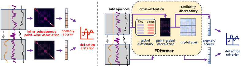
Figure 1: How to derive the detection criterion. Left: AnomalyTrans and DCdctector learn intra-subsequence point-wise association and derive the detection criterion by combining subsequence-level anomaly scores. Right: Our proposal cultivates global normal representations manifested as dictionary and prototypes for evaluating similarity discrepancy to provide series-level criterion.

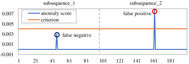
Figure 2: Anomaly scores v.s. detection criterion for different subsequences in AnomalyTrans.

As shown in Fig. 1 (left), these methods follow such pipeline to obtain the detection criterion: (a) dividing the entire series into non-overlapped subsequences (which can be seen as samples in deep learning); (b) evaluating intra-subsequence point-wise association and anomaly scores; (c) determining the unified detection criterion for all points in whatever subsequences. Therefore, such subsequence isolation approach focuses on point-wise association in limited horizon which is much less context-informative compared with the entire series. Moreover, given the heterogeneity across subsequences in terms of temporal fluctuation and the number of anomalies, the association-based point-wise anomaly scores are highly subsequence-contained. As shown in Fig. 2, directly concatenating such anomaly scores to derive the global detection criterion for the entire series results in false negative and false negative cases.

A prospective approach is to enlarge the horizon to the entire series so as to cultivate global representations shared by all normal points, which further ensures the series-level anomaly scores and detection criterion for any points. However, it is nontrivial to learn such global representations and then derive anomaly scores, given the following challenges. (1) The inherent self-attention mechanism in Transformers has the poor $\mathcal{O}(n^{2})$ time and space complexity, with $n$ denoting the number of tokens. Therefore, directly inputting the entire series, with each time point corresponding to a token, will lead to the enormous scale of attention maps, which lags the training process and challenges the memory size. (2) Supposing we obtain the well-cultivated global representations, a natural detection criterion is that the similarity discrepancy of global-abnormal representations is higher than that of the global-normal ones. Given the numerous and complex temporal representations in the entire series, the simple statistical approaches, i.e., Kullback–Leibler (KL) divergence (van Erven & Harremos, 2014) and Jensen-Shannon (JS) divergence (Fuglede & Topsoe, 2004) are incompetent to evaluate the similarity between the inherent temporal patterns.

To address these challenges, we propose a similarity-based anomaly detection method, which augments the Transformer with the global dictionary of Key and Value vectors to provide global discrete latent representations shared by all normal points. Therefore, after the cross attention operation between the Query and Key vectors, each row in the cross-attention maps can always represent the correlation weights between a given point and global representations (Key vectors). Moreover, due to the much smaller size of the global dictionary, the computational and memory efficiency will be improved in attention process. For the second challenge, we introduce prototypes to capture the normal distribution of cross-attention weights. Therefore, well-cultivated prototypes have higher discrepancy with the abnormal point-global similarity, promising an effective anomaly detection criterion. We term our model the Global Dictionary-enhanced Transformer ($\mathtt{GDformer}$), as shown in Fig. 1 (right). The contributions of the paper can be summarized as follows.

• We propose $\mathtt{GDformer}$ with a global dictionary of Key and Value vectors for learning the global representations shared by all normal points, which alleviates the effects of subsequence isolation and ensures the unified detection criterion.

• We introduce prototypes to capture the normal point-global correlation patterns, which enables distinguishable normal-abnormal similarity discrepancy and provides a compact decision boundary.

• $\mathtt{GDformer}$ achieves state-of-the-art performance on five benchmarks. Extensive experiments further validate the transferability of the global dictionary.

2 Related Work

Time series anomaly detection has been extensively studied, with massive of statistical, machine learning, and deep learning methods being proposed. The classical statistical methods learn the statistical characteristics of time series data, such as the autoregressive integrated moving average (ARIMA) approach (Box & Pierce, 1970). These methods are computation-lightweight but non-effective for complex multivariate time series anomaly detection. Machine learning methods include clustering-based, density-based, and classification-based ones. In clustering-based methods, the distance to the clustering centers is termed as the anomaly score. Various methods are proposed to obtain the temporal representations for cluster, including support vector data description(SVDD) (Tax & Duin, 2004), Deep-SVDD (Ruff et al., 2018), Temporal Hierarchical One-Class network (THOC) (Shen et al., 2020), and Integrative Tensorbased Anomaly Detection (ITAD) (Shin et al., 2020). In density-based methods, the density of temporal representations is calculated for outlier determination, including local outlier factor (LOF) (Breunig et al., 2000), connectivity outlier factor (COF) (Tang et al., 2002), Deep Autoencoding Gaussian Mixture Model (DAGMM) (Zong et al., 2018), and (mixture of probabilistic principal components analyzers and categorical distributions (MPPCACD) (Yairi et al., 2017). The classification-based methods treat time series anomaly detection as a classification task and accordingly employ the classification methods, such as decision trees (Liu et al., 2008), support vector machines (SVM) (Schölkopf et al., 2001), and one-class SVM.

Deep learning methods are roughly divided into forecasting-based and reconstruction-based ones. In the former, future values are predicted and forecasting errors are formalized as the anomaly scores. The representative methods include long short-term memory networks (LSTM) (Hundman et al., 2018b), graph neural networks (Deng & Hooi, 2021; Ding et al., 2023), and Generative Adversarial Networks (GAN) (Yao et al., 2022). Reconstruction-based methods involves reconstructing the input time series and reconstruction errors are termed as anomaly scores. In LSTM-VAE, the LSTM backbone is adopted for temporal representation and the Variational AutoEncoder (VAE) for reconstruction (Park et al., 2018). OmniAnomaly renovates LATM-VAE with reconstruction probability as anomaly score (Su et al., 2019b). In BeatGAN, the generated samples by GAN are compared with true values (Zhou et al., 2019). Another line of reconstruction-based methods do not directly employ reconstruction errors as anomaly scores, but the association-based criterion. AnomalyTrans embodies a novel anomaly-attention mechanism is proposed to learn point-wise series- and prior-association and then derives the association discrepancy-based criterion (Xu et al., 2022). In contrast, DCdetector employs contrastive learning between patch-wise and in-patch representations to increase the distribution discrepancy (Yang et al., 2023).

In these methods, Transformer (Vaswani et al., 2017) is widely used to learn temporal representations, due to its effectiveness in modeling sequential data. However, the receptive fields of Transformers largely depends on the horizons of input subsequence, resulting in the less context-informative temporal representations and inconsistent detection criterion for subsequence-specific points. By contrast, we propose the $\mathtt{GDformer}$, which goes beyond such subsequence isolation strategy and via the introduction of the dictionary-based cross-attention mechanism to cultivate global normal representations with series-level context information and derive the unified similarity-based criterion.

Figure 3: The framework of $\mathtt{GDformer}$. In Dictionary-Based Cross Attention (right), Key, Value, and Prototype are kept in memory to capture normal temporal patterns of the entire series. The cross attention module enables the unified reference for any-position points. The similarity evaluation module promises the compact distinguishable criterion.

3 Methodology

Suppose there are $d$ sensors or machines in an industrial system. The observations in the duration of $\mathcal{T}$ can be denoted as time series $\bm{\mathcal{X}}=(\bm{x}_{1},\bm{x}_{2},\dots,\bm{x}_{\mathcal{T}})$, where $\bm{x}_{t}\in\mathbb{R}^{d}$ represents these $d$ measurements at time $t$. In the context of time series anomaly detection, we need to determine whether the observation at time $t$ is anomalous or not, i.e., yielding $\bm{\mathcal{Y}}=(y_{1},y_{2},\dots,y_{\mathcal{T}})$, where $y_{t}=1$ if $x_{t}$ is anomalous and $y_{t}=0$ otherwise. In the training process, the whole time series are usually divided into overlapped or non-overlapped subsequences with $T$ time steps and then input into the designed models for representation learning. Without loss of generality, we denote $\bm{X}\in\mathbb{R}^{T\times d}$ as a subsequence.

3.1 Model Architecture

The overall structure of our proposed $\mathtt{GDformer}$ is shown in Fig. 3. Overall, $\mathtt{GDformer}$ stacks the dictionary-based cross-attention module and the feed-forward layers alternatively for representation learning, with a projection block for reconstruction. The subsequence $\bm{X}$ can be transformed into the input embedding of the first layer (details in Section 3.1.1), denoted as $\bm{X}_{0}$. The overall operations of the $l$-th layer $(l\in[1,L])$ can be formulated as:

$$\begin{array}[]{l}\bm{U}_{l}=\text{LN}(\bm{X}_{l-1}+\text{CA}(\bm{X}_{l-1},\bm{K}_{l},\bm{V}_{l})),\\ \bm{X}_{l}=\text{LN}(\bm{U}_{l}+\text{FeedForward}(\bm{U}_{l})),\end{array}$$ (1)

where LN represents the layer normalization and CA represents our proposed dictionary-based cross attention mechanism. $\bm{K}$ and $\bm{V}$ denote the learnable Key and Value vectors in the global dictionary. $\bm{U}_{l}$ denotes the hidden temporal representation. We elaborate the details of input embedding and dictionary-based cross attention in the following parts.

3.1.1 Input Embedding

For the input subsequence $\bm{X}$, we randomly mask the $T\times d$ observation values with the probability of $\alpha$. Since we aim to learn the shared representations of normal points, we do not mask (all channels of) certain points. Furthermore, we do not mask a whole channel, which guarantees the learning of multivariate dependence. Then, the masked subsequence is normalized via instance normalization (Kim et al., 2022; Ulyanov et al., 2017), denoted as $\tilde{\bm{X}}\in\mathbb{R}^{T\times d}$, to mitigate the effects of observation noise. We adopt a simple linear layer to create the input embedding $\tilde{\bm{X}}\in\mathbb{R}^{T\times D}$, where $D$ is the input dimension of the Transformer layers. We term each point $\tilde{\bm{x}}_{t}\in\mathbb{R}^{D}$ in $\tilde{\bm{X}}$ as a temporal token. Accordingly we can obtain $\bm{X}_{0}=\tilde{\bm{X}}$.

3.1.2 Dictionary-Based Cross Attention

The canonical Transformers learn the correlation of different temporal tokens via self-attention mechanism, where the triple inputs, i.e., Query, Key and, Value are all derived by the linear projection of $\tilde{\bm{X}}$ (Vaswani et al., 2017). Compared with the entire series, the subsequence $\tilde{\bm{X}}$ is constrained to fixed horizons and is less context-informative. Therefore, the cultivated temporal representations from the self-attention mechanism can only learn intra-subsequence knowledge. On the other hand, given the heterogeneity of abnormal points and temporal distribution in different subsequences, the subsequence-isolated analysis can hardly ensure the global detection criterion for all points. Hence, in this section, we devise a novel dictionary-based cross attention mechanism to foster series-level global representations shared by normal points, which naturally guarantees the unified anomaly evaluation and detection criterion.

Cross Attention. We maintain a global dictionary for each Transformer layer respectively. We suppose each layer has the same dictionary size $N$, i.e., containing $N$ Key and Value vectors. In dictionary-based cross attention block, for each head $h\in{1,2,\cdots,H}$, we define the Query matrix $\bm{Q}_{l}^{h}=\bm{X}_{l-1}W_{l}^{h}$, where $W_{l}^{h}\in\mathbb{R}^{D\times D_{h}}$ and $D_{h}=\lfloor\frac{D}{H}\rfloor$. We denote $\bm{K}_{l}\in\mathbb{R}^{N\times D}$ and $\bm{V}_{l}\in\mathbb{R}^{N\times D}$ as the $N$ Key and Value vectors of the global dictionary in the $l$-th Transformer layer. Note that we directly split $\bm{K}_{l}$ and $\bm{V}_{l}$ into $\bm{K}_{l}^{h}\in\mathbb{R}^{N\times D_{h}}$ and $\bm{V}_{l}^{h}\in\mathbb{R}^{N\times D_{h}}$ for each head $h$, instead of using linear projection layers. The operation of cross-attention in head $h$ can be defined as:

$$\bm{U}_{l}^{h}={\rm Softmax}(\frac{\bm{Q}_{l}^{h}\bm{K}_{l}^{h\top}}{\sqrt{D_{h}}})\bm{V}_{l}^{h}.$$ (2)

Then, We can fuse $\bm{U}_{l}^{h}\in\mathbb{R}^{T\times D_{h}}$ in each head to obtain $\bm{U}_{l}\in\mathbb{R}^{T\times D_{h}}$, which are adopted for reconstruction. In the unsupervised training process, $\bm{K}_{l}$ and $\bm{V}_{l}$ are updated iteratively with all temporal points, which can learn the shared representations of normal points in the entire series.

The calculation complexity of the dictionary-based cross attention mechanism is formulated as $\mathcal{O}(TN)$, which is much less than that of the original self-attention mechanism (formulated as $\mathcal{O}(T^{2})$), given the dictionary size $N$ much lower than the subsequence length $T$. Therefore, the introduction of dictionary can improve the computation and memory efficiency. Detailed comparison results can be found in Section 4.2.2 and Appendix E.

Let $\bm{M}_{l}^{h}={\rm Softmax}(\frac{\bm{Q}_{l}^{h}\bm{K}_{l}^{h\top}}{\sqrt{D_{h}}})$ denote the cross-attention weights. Each row in $\bm{M}_{l}^{h}\in\mathbb{R}^{T\times N}$ reflects the distribution of correlation weights between each temporal representation and the global representation $\bm{K}_{l}^{h}$. We can directly compare the discrepancy of such distribution and then determine a detection criterion. However, the conventional methods mainly adopt statistics methods such as KL divergence and JS divergence to evaluate distribution similarity, which is susceptible to outliers, hardly guaranteeing compact decision boundary (comparison results in Section 4.2.1). Therefore, in our devised dictionary-based cross attention mechanism, besides a branch for reconstruction, we introduce an extra branch for similarity discrepancy.

Note that the global dictionary can learn the global representations shared by the normal points in the entire series. As for the research of foundation models in time series analysis, one can train a unified model for cross-domain time series datasets (Liang et al., 2024). Furthermore, we have a key observation that the global dictionary have great transferability (details in Section 4.1), which validates that cross-domain datasets may have the shared normal temporal patterns, thus laying the foundation for the construction of time series anomaly detection foundation model.

Similarity Evaluation. In this section, we aim at evaluating the similarity between representations from the perspective of the inherent temporal patterns, instead of distribution difference, which can guarantee the diverse normal representations in the entire series have higher similarity with the global representations, thus deriving the compact detection criterion. We maintain $P$ prototypes for each Transformer layer to capture the distribution patterns of normal-global correlation weights, which can be denoted as $\bm{E}_{l}\in\mathbb{R}^{P\times N}$ in the $l$-th layer. Then, we calculate the similarity between $\bm{E}_{l}$ and $\bm{M}_{l}^{h}$ as:

$$\bm{S}_{l}^{h}=\bm{M}_{l}^{h}{\rm Softmax}(\bm{E}_{l})^{\top},$$ (3)

where we first normalize the prototypes via ${\rm Softmax}(\bm{E}_{l})$. Each row in $\bm{S}_{l}^{h}\in\mathbb{R}^{T\times P}$ represents the similarity between the point-global correlation distribution (in $\bm{M}_{l}^{h}$) and the prototypical distribution patterns $\bm{E}_{l}$. We then fuse $\bm{S}_{l}^{h}$ by row to obtain $\hat{\bm{S}}_{l}^{h}\in\mathbb{R}^{T}$, where each scalar represents the similarity strength of the corresponding point. Higher values reflect stronger similarity between the correlation weights and prototypes, naturally promising a similarity-based criterion. Detailed process of dictionary-based cross-attention mechanism is presented in Appendix B.

3.2 Training and Inference

We adopt the reconstruction loss to guide the global dictionary to learn the shared representations of the series-level normal points. To further guarantee prototypes learn the normal distribution patterns, the similarity loss between the cross-attention weights and prototypes is introduced, which can be formulated as:

$${\mathcal{L}_{total}} ={\mathcal{L}_{c}}-\lambda{\mathcal{L}_{s}}$$

$$=\left\|{\bm{X}-\hat{\bm{X}}}\right\|_{2}^{2}-\lambda{\left\|{\sum\nolimits_{l}{\sum\nolimits_{h}{\hat{\bm{S}}_{l}^{h}}}}\right\|_{1}},$$ (4)

where $\hat{\bm{X}}\in\mathbb{R}^{T\times d}$ denotes the reconstruction results of $\bm{X}$. $\mathcal{L}_{c}$ and $\mathcal{L}_{s}$ represent the reconstruction loss and the similarity discrepancy loss respectively. $\|\cdot\|_{*}$ denotes the $*$-norm. $\lambda$ is adopted to balance the two loss items. We set $\lambda>0$ to enlarge the similarity degree between the prototypes and the cross-attention weights in unsupervised learning. We can observe that $\mathcal{L}_{s}$ sums the similarity values in all $L$ layers and can aggregate multi-scale distribution knowledge, thereby leading to an informative measure.

Table 1: Anomaly detection performance comparisons. All metrics are organized in %. Bold: the best. Underline: the second best.

Dataset	SMD			MSL			SMAP			SWaT			PSM
Metric	P	R	F1	P	R	F1	P	R	F1	P	R	F1	P	R	F1
OCSVM	44.34	76.72	56.19	59.78	86.87	70.82	53.85	59.07	56.34	45.39	49.22	47.23	62.75	80.89	70.67
IForest	42.31	73.29	53.64	53.94	86.54	66.45	52.39	59.07	55.53	49.29	44.95	47.02	76.09	92.45	83.48
LOF	56.34	39.86	46.68	47.72	85.25	61.18	58.93	56.33	57.60	72.15	65.43	68.62	57.89	90.49	70.61
MMPCACD	71.20	79.28	75.02	81.42	61.31	69.95	88.61	75.84	81.73	82.52	68.29	74.73	76.26	78.35	77.29
DAGMM	67.30	49.89	57.30	89.60	63.93	74.62	86.45	56.73	68.51	89.92	57.84	70.40	93.49	70.03	80.08
Deep-SVDD	78.54	79.67	79.10	91.92	76.63	83.58	89.93	56.02	69.04	80.42	84.45	82.39	95.41	86.49	90.73
THOC	79.76	90.95	84.99	88.45	90.97	89.69	92.06	89.34	90.68	83.94	86.36	85.13	88.14	90.99	89.54
ITAD	86.22	73.71	79.48	69.44	84.09	76.07	82.42	66.89	73.85	63.13	52.08	57.08	72.80	64.02	68.13
BOCPD	70.90	82.04	76.07	80.32	87.20	83.62	84.65	85.85	85.24	89.46	70.75	79.01	80.22	75.33	77.70
U-Time	65.95	74.75	70.07	57.20	71.66	63.62	49.71	56.18	52.75	46.20	87.94	60.58	82.85	79.34	81.06
TS-CP2	87.42	66.25	75.38	86.45	68.48	76.42	87.65	83.18	85.36	81.23	74.10	77.50	82.67	78.16	80.35
LSTM	78.55	85.28	81.78	85.45	82.50	83.95	89.41	78.13	83.39	86.15	83.27	84.69	76.93	89.64	82.80
CL-MPPCA	82.36	76.07	79.09	73.71	88.54	80.44	86.13	63.16	72.88	76.78	81.50	79.07	56.02	99.93	71.80
LSTM-VAE	75.76	90.08	82.30	85.49	79.94	82.62	92.20	67.75	78.10	76.00	89.50	82.20	73.62	89.92	80.96
BeatGAN	72.90	84.09	78.10	89.75	85.42	87.53	92.38	55.85	69.61	64.01	87.46	73.92	90.30	93.84	92.04
OmniAnomaly	83.68	86.82	85.22	89.02	86.37	87.67	92.49	81.99	86.92	81.42	84.30	82.83	88.39	74.46	80.83
InterFusion	87.02	85.43	86.22	81.28	92.70	86.62	89.77	88.52	89.14	80.59	85.58	83.01	83.61	83.45	83.52
AnomalyTrans	88.47	92.28	90.33	91.92	96.03	93.93	93.59	99.41	96.41	89.10	99.28	94.22	96.94	97.81	97.37
DCdetector	83.59	91.10	87.18	92.28	97.21	94.68	94.25	98.59	96.37	93.11	99.77	96.33	97.14	98.74	97.94
$\mathtt{GDformer}$	86.33	94.89	90.41	93.70	98.07	95.83	95.55	97.52	96.52	96.28	99.82	98.02	97.97	99.52	98.74

Anomaly Detection Criterion. After optimization, the prototypes can learn the distribution of the correlation weights between normal temporal representations and the global representations. Therefore, the similarity values of abnormal attention weights and prototypes are lower than those of normal ones. Naturally, in inference process, we can obtain the anomaly score of $\bm{X}\in\mathbb{R}^{T\times d}$ as:

$${\rm AnomalyScore}(\bm{X})={\rm Softmax}\left(-{\sum\nolimits_{l}{\sum\nolimits_{h}{\hat{\bm{S}}_{l}^{h}}}}\right),$$ (5)

where ${\rm AnomalyScore}(\bm{X})\in\mathbb{R}^{T}$ indicates the point-wise anomaly scores for $T$ points and has higher values for abnormal points. Let $\delta$ denote the series-level anomaly threshold. We can obtain the detection output $\bm{\mathcal{Y}}$ as:

$${y_{i}}(i\in[1,\mathcal{T}])=\left\{{\begin{array}[]{*{20}{c}}{1,}&{{\rm AnomalyScore}{{(\bm{x}_{i})}}\geq\delta,}\\ {0,}&{{\rm AnomalyScore}{{(\bm{x}_{i})}}<\delta.}\end{array}}\right.$$ (6)

4 Experiments

Our baselines cover a broad collection of relevant methods, including the classic methods: OCSVM (Tax & Duin, 2004) and IForest (Liu et al., 2008); density-estimation models: LOF (Breunig et al., 2000), MPPCACD (Yairi et al., 2017), and DAGMM (Zong et al., 2018); clustering-based models: Deep-SVDD (Ruff et al., 2018), THOC (Shen et al., 2020), and ITAD (Shin et al., 2020); time series segmentation methods: BOCPD (Adams & MacKay, 2007), U-Time (Perslev et al., 2019), and TS-CP2 (Deldari et al., 2021); autoregression-based models: LSTM (Hundman et al., 2018b) and CL-MPPCA (Tariq et al., 2019); reconstruction-based models: LSTM-VAE (Park et al., 2018), BeatGAN (Zhou et al., 2019), OmniAnomaly (Su et al., 2019b), InterFusion (Li et al., 2021b), AnomalyTrans (Xu et al., 2022), and DCdetector (Yang et al., 2023). We directly cite the results from (Yang et al., 2023) if applicable.

We evaluate on 5 real-world benchmark datasets from various domains: SMD, MSL, SMAP, SWaT, and PSM. More details of the datasets and implementation can be found in Appendix A. The adopted metrics include precision (P), recall (R), and F1-score.

Table 2: Transfer results of $\mathtt{GDformer}$. All metrics are organized in %. Bold: the best. Underline: the second best.

Metric		P	R	F1
AnomalyTrans		96.94	97.81	97.37
DCdetector		97.14	98.74	97.94
$\mathtt{GDformer}$	PSM $\Rightarrow$ PSM	97.97	99.52	98.74
	SMAP$\Rightarrow$PSM	97.97	98.36	98.16
	MSL$\Rightarrow$PSM	98.48	97.56	98.02
	SWaT$\Rightarrow$PSM	98.36	97.22	97.79
AnomalyTrans		89.10	99.28	94.22
DCdetector		93.11	99.77	96.33
$\mathtt{GDformer}$	SWaT$\Rightarrow$SWaT	96.28	99.82	98.02
	SMAP$\Rightarrow$SWaT	95.39	99.82	97.55
	MSL$\Rightarrow$SWaT	94.16	98.97	96.50
	PSM$\Rightarrow$SWaT	94.93	99.82	97.31
AnomalyTrans		91.92	96.03	93.93
DCdetector		92.28	97.21	94.68
$\mathtt{GDformer}$	MSL$\Rightarrow$MSL	93.70	98.07	95.83
	SMAP$\Rightarrow$MSL	92.78	97.03	94.86
	SWaT$\Rightarrow$MSL	92.76	98.07	95.34
	PSM$\Rightarrow$MSL	92.78	98.07	95.35
AnomalyTrans		93.59	99.41	96.41
DCdetector		94.25	98.59	96.37
$\mathtt{GDformer}$	SMAP$\Rightarrow$SMAP	95.55	97.52	96.52
	MSL$\Rightarrow$SMAP	94.38	96.57	95.46
	SWaT$\Rightarrow$SMAP	94.69	97.87	96.25
	PSM$\Rightarrow$SMAP	94.64	96.63	95.62

4.1 Main Results

We compare the anomaly detection performance of our $\mathtt{GDformer}$ with the 19 popular baselines on 5 benchmark datasets. The numerical results are reported in Table 1. We can observe that $\mathtt{GDformer}$ consistently outperforms the baselines on all datasets. Compared with state-of-the-art methods, AnomalyTrans and DCdetector, which adopts association discrepancy as detection criterion, our proposed $\mathtt{GDformer}$ can cultivate more context-informative representations and promise a compact detection criterion, thus facilitating performance gains.

Table 3: Ablation results (F1-score) in $\mathcal{L}_{c}$ and $\mathcal{L}_{s}$, and anomaly detection criterion. The module is remarked with “✗”, if we ablate it and “✓” otherwise. self-attention and cross-attention represent attention maps are from self-attention or dictionary-based cross attention mechanism. Recon and SimDis represent the reconstruction error or the similarity discrepancy-based criterion. Bold: the best.

Variant	$\mathcal{L}_{c}$	$\mathcal{L}_{s}$	Criterion	MSL	SWaT	PSM	SMAP	Avg
A.1	self-attention	✗	Recon	88.94	94.29	93.72	76.76	88.43
A.2	self-attention	✓	Recon	88.61	94.04	92.84	72.59	87.02
A.3	self-attention	✓	SimDis	92.33	93.35	97.70	82.24	91.41
A.4	cross-attention	✓	Recon	90.84	93.00	92.79	76.04	88.17
A.5	✗	✓	SimDis	95.21	94.65	98.03	75.69	90.90
A.6 $\mathtt{GDformer}$	cross-attention	✓	SimDis	95.83	98.02	98.74	96.52	97.28

Table 4: Ablation results in $\mathcal{L}_{s}$, i.e., similarity evaluation. Bold: the best.

Dataset	MSL			SWaT			PSM			SMAP
Metric	P	R	F1	P	R	F1	P	R	F1	P	R	F1
B.1	92.75	91.63	92.19	95.84	94.29	95.06	98.48	96.72	97.59	96.58	96.32	96.45
B.2	92.34	81.77	86.73	95.78	92.97	94.36	98.63	95.69	97.14	94.72	60.88	74.12
C.1	93.20	93.05	93.12	96.21	97.95	97.07	98.46	95.86	97.14	94.69	63.83	76.26
C.2	93.35	93.46	93.40	95.94	94.26	95.10	98.57	96.08	97.31	94.27	57.40	71.36
$\mathtt{GDformer}$	93.70	98.07	95.83	96.28	99.82	98.02	97.97	99.52	98.74	95.55	97.52	96.52

Transferability. We evaluate the transferability of the global dictionary and prototypes across datasets. These two objects are frozen and transferred to ♣, after they are optimized on ♠. The transfer performance (“♠$\Rightarrow$♣”) is reported in Table 2. The transfer performance of $\mathtt{GDformer}$ is consistently superior to AnomalyTrans and DCdetector on all datasets, except for SMAP. Compared with “♣$\Rightarrow$♣” settings, the transfer performance has little F1-score reduction. It indicates that the normal points may have shared temporal representations and patterns even cross different datasets.

4.2 Model Analysis

4.2.1 Ablation Study

Model Ablation. The ablation results of loss function and detection criterion are shown in Table 3. The proposed similarity-based criterion brings 9.11% averaged F1-score improvements (from 88.17% to 97.28%), by comparing A.4 and A.6. The proposed dictionary-based cross attention mechanism can provide 5.87% averaged F1-score improvements (from 91.41% to 97.28%) by comparing A.3 and A.6. In A.5, we employ dictionary-based cross attention mechanism to obtain the attention map but ablate $\mathcal{L}_{c}$ from Eq. (4). A.5 achieves better performance compared with A.1, the pure Transformer, which validates our insight that similarity discrepancy might be a promising alternative to the reconstruction error in time series anomaly detection.

Similarity Evaluation Ablation. We conduct ablation studies on similarity discrepancy loss $\mathcal{L}_{s}$ and the numerical results are presented in Table 4. As is formulated in Eq. (4), $\mathcal{L}_{s}$ combines the cosine similarity in all $L$ layers. B.1 (B.2) means only the first one (two) layer(s) is (are) considered in Eq. (4). C.1 and C.2 mean we adopt KL divergence and JD divergence respectively in Eq. (3) to calculate the map-prototype similarity. As is shown in Table 4, all-layer combination achieves the best, due to the effective usage of multi-level features. Compared with C.1 and C.2, $\mathtt{GDformer}$ is more possible to cultivate the diversity of the prototypes, thereby effectively capturing the attention weights of normal-global representations. Therefore, $\mathtt{GDformer}$ outperforms C.1 and C.2.

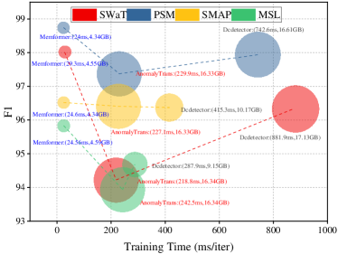
Figure 4: Model efficiency comparison in terms of training time, F1 score, and memory footprint. Larger bubble size indicates higher memory requirements.

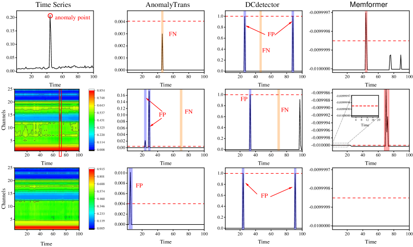
Figure 5: Detection results visualization of AnomalyTrans, DCdetector, and $\mathtt{GDformer}$ on PSM dataset. The point and segment anomalies are marked in red circles and red segments. We plot the detection scores for different methods and the corresponding detection threshold (red dashed lines). FP (false positive), FN (false negative) and true positive are highlighted in blue, yellow and red respectively.

4.2.2 Model Efficiency

We compare the model efficiency in terms of detection accuracy, training time, and memory footprint of the following methods: AnomalyTrans, DCdetector, and $\mathtt{GDformer}$. As shown in Fig. 4, our proposed $\mathtt{GDformer}$ exceeds the other two Transformer-based methods consistently on four datasets. In self-attention module, the complexity can be formalized to $\mathcal{O}(T^{2})$. While in the devised coss-attention module, the complexity is $\mathcal{O}(TN)$, with $N$ much smaller than $T$ in our experiments. Hence, the memory footprints of $\mathtt{GDformer}$ are lower than those of AnomalyTrans and DCdetector. Moreover, the two baselines involve two-branch association modeling and two-stage optimization, which slows the training process. In contrast, in $\mathtt{GDformer}$, the training time decreases significantly, with 88.8% and 94.7% averaged decline w.r.t AnomalyTrans and DCdetector.

4.2.3 Case Study

We showcase the detection results under the point and segment anomalies in Fig. 5. We visualize one selected dimension for the point anomaly in the first row. We can observe that AnomalyTrans and DCdetector fail to detect such point anomaly with the corresponding detection scores lower than anomaly criteria. Moreover, DCdetector even generates false positive cases. The second row shows the segment anomalies. We visualize the multivariate time series via a contour plot. It is clear that anomaly points range from 70 to 72. $\mathtt{GDformer}$ can consistently detect the segment anomalies. By contrast, the two baselines generate false cases. In the third row, no anomalies exist in the input series, but the two baselines both yield false positive cases. In general, AnomalyTrans and DCdetector focus on intra-subsequence point-wise association divergence, which is prone to be affected by the subsequence heterogeneity, and fail to promise compact series-level criteria, thus generating false cases. $\mathtt{GDformer}$ can cultivate global representations with series-level knowledge and provide the unified criterion for any-position representations.

5 Conclusion and Future Work

This paper proposes the global dictionary-enhanced Transformer model, $\mathtt{GDformer}$, to foster the learning of global representations shared by all normal points, which can solve the problem of limited horizons faced by the canonical Transformer. Specifically, we renovate the self-attention mechanism into the dictionary-based cross-attention mechanism, where the Key and Value vectors in the global dictionary can learn the shared temporal representations. Moreover, the prototypes are introduced to capture the similarity distribution of normal points manifested by the cross-attention weights, which derives the similarity-based criterion. Extensive experiments validate the state-of-the-art performance of $\mathtt{GDformer}$. The theoretical analysis on the functions of key-value pairs in the dictionary-based cross-attention mechanism will be conducted in the future work. Moreover, given the transferability, we will explore the construction of foundation models for anomaly detection.

Impact Statements

This paper presents work whose goal is to advance the field of Machine Learning. There are many potential societal consequences of our work, none which we feel must be specifically highlighted here.

Appendix A Implementation Details

Datasets. We evaluate the anomaly detection performance on 5 real-world datasets: (1) SMD (Server Machine Dataset) is collected from an Internet company with 38 dimensions (Su et al., 2019a). (2) MSL (Mars Science Laboratory dataset) is collected by NASA with 55 dimensions and shows the condition of the sensors and actuator data from the Mars rover (Hundman et al., 2018a). (3) SMAP (Soil Moisture Active Passive dataset) is also collected from NASA with 25 dimensions and records the soil samples of Mars (Hundman et al., 2018a). (4) SWaT (Secure Water Treatment dataset) is collected from the critical infrastructure systems with 51 sensors (Mathur & Tippenhauer, 2016). (5) PSM (Pooled Server Metrics dataset) is collected from eBay server machines with 25 dimensions (Abdulaal et al., 2021). More details are reported in Table 5.

Experimental Settings. We comply with the settings of (Xu et al., 2022) to divide the whole series into multiple non-overlapped subsequences with $T=100$. For $\mathtt{GDformer}$, we have $L=3$, the embedding dimension $D=512$, the number of cross-attention heads $H=8$. The mask ratio $\alpha$ is set to $5\%$. The settings of the dictionary size $N$, the number of prototypes $P$, the loss trade-off parameter $\lambda$, and the threshold $\delta$ are dataset-variant, which is shown in 5. We employ the ADAM (Kingma & Ba, 2015) with an initial learning rate of $10^{-4}$ to optimize model parameters. The training process is continued for 10 epochs with the batch size of 64. All experiments are implemented in PyTorch (Paszke et al., 2019) with a single NVIDIA GeForce RTX 3090 24GB GPU.

Table 5: Datasets’ details and optimal hyperparameter settings. AR: the abnormal proportion of the whole dataset.

Dataset	Domain	Dimension	Window	#Training	#Validation	#Test	AR	$\lambda$	$P$	$N$	$\delta$
SMD	Server	38	100	566,724	141,681	708,420	0.042	1	16	16	0.7
MSL	Space	55	100	46,653	11,664	73,729	0.105	3	12	16	0.8
SMAP	Space	25	100	108,146	27,037	427,617	0.128	2	12	6	0.7
SWaT	Water	51	100	396,000	99,000	449,919	0.121	2	8	8	0.5
PSM	Server	25	100	105,984	26,497	87,841	0.278	1	10	10	0.6

Appendix B Process of Dictionary-based Cross Attention

Algorithm 1 Dictionary-based Cross Attention Mechanism

1: Input:$\bm{X}_{l-1}\in\mathbb{R}^{T\times D}$; initialized dictionary: $\bm{K}_{l}^{h}\in\mathbb{R}^{N\times D_{h}}$, $\bm{V}_{l}^{h}\in\mathbb{R}^{N\times D_{h}}$ ($h\in[1,H]$), and $\bm{E}_{l}\in\mathbb{R}^{P\times N}$

2: for $h\in[1,H]$ do

3:  $\bm{Q}_{l}^{h}=\bm{X}_{l-1}\bm{W}_{l}^{h}$ $\triangleright$ $\bm{W}_{l}^{h}\in\mathbb{R}^{D\times D_{h}},\bm{Q}_{l}^{h}\in\mathbb{R}^{T\times D_{h}}$

4:  $\bm{M}_{l}^{h}={\rm Softmax}(\frac{\bm{Q}_{l}^{h}\bm{K}_{l}^{h\top}}{\sqrt{D_{h}}}),\bm{U}_{l}^{h}=\bm{M}_{l}^{h}\bm{V}_{l}^{h}$ $\triangleright$ $\bm{M}_{l}^{h}\in\mathbb{R}^{T\times N},\bm{U}_{l}^{h}\in\mathbb{R}^{T\times D_{h}}$: output for reconstruction

5:  $\bm{S}_{l}^{h}=\bm{M}_{l}^{h}{\rm Softmax}(\bm{E}_{l})^{\top}$ $\triangleright$ $\bm{S}_{l}^{h}\in\mathbb{R}^{T\times P}$: similarity between two distributions

6:  $\hat{\bm{S}}_{l}^{h}={\rm Sum}(\bm{S}_{l}^{h},{\rm dim}=1)$ $\triangleright$ $\hat{\bm{S}}_{l}^{h}\in\mathbb{R}^{T}$: the similarity values w.r.t prototypes

7: end for

8: $\bm{U}_{l}={\rm Concat}([\bm{U}_{l}^{1},\cdots,\bm{U}_{l}^{H}],{\rm dim}=1)$ $\triangleright$ $\bm{U}_{l}\in\mathbb{R}^{T\times D}$

9: $\hat{\bm{S}}_{l}={\rm Sum}([\hat{\bm{S}}_{l}^{1},\cdots,\hat{\bm{S}}_{l}^{H}],{\rm dim}=1)$ $\triangleright$ $\hat{\bm{S}}_{l}\in\mathbb{R}^{T}$

10: Return $\bm{U}_{l}$ and $\hat{\bm{S}}_{l}$ $\triangleright$ $\bm{U}_{l}$ for reconstruction; $\hat{\bm{S}}_{l}$ for similarity discrepancy

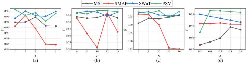
Figure 6: Parameter sensitivity analysis of (a) loss weight $\lambda$, (b) prototype size $P$, (c) dictionary size $N$, and (d) detection threshold $\delta$.

Appendix C Sensitivity Investigation

We analyze the effects of different settings of hyperparameters on the detection performance, including the loss weight $\lambda$, number of prototypes $P$, dictionary size $N$, and detection threshold $\delta$. Fig. 6 shows the F1-score sensitivity on the four datasets. It is explicit that we cannot conclude the same setting, due to the data heterogeneity across different datasets. The loss weight $\lambda$ in Eq. (4) is adopted to trade off the reconstruction loss and the distribution discrepancy loss. Higher values of $\lambda$ do not always guarantee higher F1-scores. We find that [1,3] may be an optimal range for all datasets. Higher values of $P$ and $N$ have larger memory requirements. Less prototypes or key-value pairs may fail to memorize the normal temporal patterns. On the other hand, more will redundant information, which subsequently leads to loose boundary. We have the observation that how we design $\mathcal{L}_{s}$ have stronger effects on SMAP compared with the other three datasets, given F1-score on SMAP varies significantly with different settings of $\lambda$, $P$, and $N$. $\delta$ indicates the top $\delta\%$ anomaly score is termed as the detection criterion, which is dataset-specific.

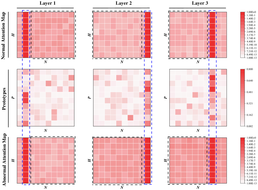
Figure 7: The showcase of prototypes (the second row) and attention maps on normal (the first row) and abnormal points (the third row). Each column corresponds to a layer. Each row corresponds to the same color bar.

Appendix D More Showcase

Fig. 7 shows the prototypes and cross-attention scores of the normal and abnormal points. We have the key observation that the prototypical distribution of the association weights is unimodal in all layers. Moreover, in the blue dashed box, the cross-attention scores of the normal and abnormal points are both in line with the above observation. Therefore, directly adopting reconstruction errors as the detection criterion may lead to inferior accuracy. While the distribution of attention scores in the black dashed box vary on normal and abnormal points. Specifically, in the first layer, the weights in black dashed box of the normal point are higher than those of the abnormal point, which is the opposite case for the second and third layers. Hence, it naturally results in a distribution similarity-based criterion.

Appendix E More Analysis

Given the same model settings with the Transformer dimension denoted as $D$ and $H$ heads, the number of parameters in one Anomaly-Attention layer (Xu et al., 2022) is formulated as :

$$3D\times({D_{h}}\times H)+D\times H,$$ (7)

where the first addend corresponds to multi-head self-attention and the second to the prior-association. The number of parameters in the one attention layer in DCdetector (Yang et al., 2023) is formuated as:

$$3D\times({D_{h}}\times H).$$ (8)

We can obtain the parameter amount of the dictionary-based cross-attention as:

$$D\times({D_{h}}\times H)+2N\times({D_{h}}\times H)+P\times N,$$ (9)

where the first addend correspond to the input projection for Query and the second to the learnable Key-Value matrices and the last to the prototypes.

In our implementation, we have the number of prototypes $P$ and the dictionary size $N$ much less than the Transformer dimension $D$, i.e., $P\ll D,N\ll D$. Therefore, we can obtain the following derivations:

$$P\times N\ll D\times N<D\times(D-N)<2D\times(D-N)=2(D-N)\times{D_{h}}\times H.$$ (10)

Therefore,

$$P\times N+2N\times{D_{h}}\times H\ll 2D\times{D_{h}}\times H.$$ (11)

Finally, we can obtain

$$D\times{D_{h}}\times H+2N\times({D_{h}}\times H)+P\times N\ll 3D\times{D_{h}}\times H.$$ (12)

That is, given the same parameter settings of the attention layer, the parameter amount of $\mathtt{GDformer}$ is much less than those of AnomalyTrans and DCdetector.

References

- Abdulaal et al. (2021) Abdulaal, A., Liu, Z., and Lancewicki, T. Practical approach to asynchronous multivariate time series anomaly detection and localization. In Proceedings of the 27th ACM SIGKDD Conference on Knowledge Discovery & Data Mining, KDD ’21, pp. 2485–2494, New York, NY, USA, 2021. Association for Computing Machinery. ISBN 9781450383325. doi: 10.1145/3447548.3467174. URL https://doi.org/10.1145/3447548.3467174.
- Adams & MacKay (2007) Adams, R. P. and MacKay, D. J. Bayesian online changepoint detection. arXiv preprint arXiv:0710.3742, 2007.
- Box & Pierce (1970) Box, G. E. and Pierce, D. A. Distribution of residual autocorrelations in autoregressive-integrated moving average time series models. Journal of the American statistical Association, 65(332):1509–1526, 1970.
- Breunig et al. (2000) Breunig, M. M., Kriegel, H.-P., Ng, R. T., and Sander, J. Lof: identifying density-based local outliers. In Proceedings of the 2000 ACM SIGMOD international conference on Management of data, pp. 93–104, 2000.
- Deldari et al. (2021) Deldari, S., Smith, D. V., Xue, H., and Salim, F. D. Time series change point detection with self-supervised contrastive predictive coding. In Proceedings of the Web Conference 2021, pp. 3124–3135, 2021.
- Deng & Hooi (2021) Deng, A. and Hooi, B. Graph neural network-based anomaly detection in multivariate time series. In Proceedings of the AAAI conference on artificial intelligence, volume 35, pp. 4027–4035, 2021.
- Ding et al. (2023) Ding, C., Sun, S., and Zhao, J. Mst-gat: A multimodal spatial–temporal graph attention network for time series anomaly detection. Information Fusion, 89:527–536, 2023.
- Fuglede & Topsoe (2004) Fuglede, B. and Topsoe, F. Jensen-shannon divergence and hilbert space embedding. In International Symposium onInformation Theory, 2004. ISIT 2004. Proceedings., pp. 31–, 2004. doi: 10.1109/ISIT.2004.1365067.
- Hundman et al. (2018a) Hundman, K., Constantinou, V., Laporte, C., Colwell, I., and Soderstrom, T. Detecting spacecraft anomalies using lstms and nonparametric dynamic thresholding. In Proceedings of the 24th ACM SIGKDD International Conference on Knowledge Discovery & Data Mining, KDD ’18, pp. 387–395, New York, NY, USA, 2018a. Association for Computing Machinery. ISBN 9781450355520. doi: 10.1145/3219819.3219845. URL https://doi.org/10.1145/3219819.3219845.
- Hundman et al. (2018b) Hundman, K., Constantinou, V., Laporte, C., Colwell, I., and Soderstrom, T. Detecting spacecraft anomalies using lstms and nonparametric dynamic thresholding. In Proceedings of the 24th ACM SIGKDD international conference on knowledge discovery & data mining, pp. 387–395, 2018b.
- Kim et al. (2022) Kim, T., Kim, J., Tae, Y., Park, C., Choi, J.-H., and Choo, J. Reversible instance normalization for accurate time-series forecasting against distribution shift. In International Conference on Learning Representations, 2022. URL https://openreview.net/forum?id=cGDAkQo1C0p.
- Kingma & Ba (2015) Kingma, D. P. and Ba, J. Adam: A method for stochastic optimization. In Bengio, Y. and LeCun, Y. (eds.), 3rd International Conference on Learning Representations, ICLR 2015, San Diego, CA, USA, May 7-9, 2015, Conference Track Proceedings, 2015. URL http://arxiv.org/abs/1412.6980.
- Li et al. (2021a) Li, X., Shi, Q., Hu, G., Chen, L., Mao, H., Yang, Y., Yuan, M., Zeng, J., and Cheng, Z. Block access pattern discovery via compressed full tensor transformer. In Proceedings of the 30th ACM International Conference on Information & Knowledge Management, pp. 957–966, 2021a.
- Li et al. (2023) Li, Y., Chen, W., Chen, B., Wang, D., Tian, L., and Zhou, M. Prototype-oriented unsupervised anomaly detection for multivariate time series. In Proceedings of the 40th International Conference on Machine Learning, ICML’23. JMLR.org, 2023.
- Li et al. (2021b) Li, Z., Zhao, Y., Han, J., Su, Y., Jiao, R., Wen, X., and Pei, D. Multivariate time series anomaly detection and interpretation using hierarchical inter-metric and temporal embedding. In Proceedings of the 27th ACM SIGKDD conference on knowledge discovery & data mining, pp. 3220–3230, 2021b.
- Liang et al. (2024) Liang, Y., Wen, H., Nie, Y., Jiang, Y., Jin, M., Song, D., Pan, S., and Wen, Q. Foundation models for time series analysis: A tutorial and survey. In Proceedings of the 30th ACM SIGKDD conference on knowledge discovery and data mining, pp. 6555–6565, 2024.
- Liu et al. (2008) Liu, F. T., Ting, K. M., and Zhou, Z.-H. Isolation forest. In 2008 eighth ieee international conference on data mining, pp. 413–422. IEEE, 2008.
- Mathur & Tippenhauer (2016) Mathur, A. P. and Tippenhauer, N. O. Swat: a water treatment testbed for research and training on ics security. In 2016 International Workshop on Cyber-physical Systems for Smart Water Networks (CySWater), pp. 31–36, 2016. doi: 10.1109/CySWater.2016.7469060.
- Park et al. (2018) Park, D., Hoshi, Y., and Kemp, C. C. A multimodal anomaly detector for robot-assisted feeding using an lstm-based variational autoencoder. IEEE Robotics and Automation Letters, 3(3):1544–1551, 2018.
- Paszke et al. (2019) Paszke, A., Gross, S., Massa, F., Lerer, A., Bradbury, J., Chanan, G., Killeen, T., Lin, Z., Gimelshein, N., Antiga, L., Desmaison, A., Kopf, A., Yang, E., DeVito, Z., Raison, M., Tejani, A., Chilamkurthy, S., Steiner, B., Fang, L., Bai, J., and Chintala, S. Pytorch: An imperative style, high-performance deep learning library. In Wallach, H., Larochelle, H., Beygelzimer, A., d'Alché-Buc, F., Fox, E., and Garnett, R. (eds.), Advances in Neural Information Processing Systems, volume 32. Curran Associates, Inc., 2019. URL https://proceedings.neurips.cc/paper_files/paper/2019/file/bdbca288fee7f92f2bfa9f7012727740-Paper.pdf.
- Perslev et al. (2019) Perslev, M., Jensen, M., Darkner, S., Jennum, P. J., and Igel, C. U-time: A fully convolutional network for time series segmentation applied to sleep staging. Advances in Neural Information Processing Systems, 32, 2019.
- Ruff et al. (2018) Ruff, L., Vandermeulen, R., Goernitz, N., Deecke, L., Siddiqui, S. A., Binder, A., Müller, E., and Kloft, M. Deep one-class classification. In International conference on machine learning, pp. 4393–4402. PMLR, 2018.
- Schölkopf et al. (2001) Schölkopf, B., Platt, J. C., Shawe-Taylor, J., Smola, A. J., and Williamson, R. C. Estimating the support of a high-dimensional distribution. Neural computation, 13(7):1443–1471, 2001.
- Shen et al. (2020) Shen, L., Li, Z., and Kwok, J. Timeseries anomaly detection using temporal hierarchical one-class network. Advances in Neural Information Processing Systems, 33:13016–13026, 2020.
- Shin et al. (2020) Shin, Y., Lee, S., Tariq, S., Lee, M. S., Jung, O., Chung, D., and Woo, S. S. Itad: integrative tensor-based anomaly detection system for reducing false positives of satellite systems. In Proceedings of the 29th ACM international conference on information & knowledge management, pp. 2733–2740, 2020.
- Su et al. (2019a) Su, Y., Zhao, Y., Niu, C., Liu, R., Sun, W., and Pei, D. Robust anomaly detection for multivariate time series through stochastic recurrent neural network. In Proceedings of the 25th ACM SIGKDD International Conference on Knowledge Discovery & Data Mining, KDD ’19, pp. 2828–2837, New York, NY, USA, 2019a. Association for Computing Machinery. ISBN 9781450362016. doi: 10.1145/3292500.3330672. URL https://doi.org/10.1145/3292500.3330672.
- Su et al. (2019b) Su, Y., Zhao, Y., Niu, C., Liu, R., Sun, W., and Pei, D. Robust anomaly detection for multivariate time series through stochastic recurrent neural network. In Proceedings of the 25th ACM SIGKDD international conference on knowledge discovery & data mining, pp. 2828–2837, 2019b.
- Su et al. (2022) Su, Y., Zhao, Y., Sun, M., Zhang, S., Wen, X., Zhang, Y., Liu, X., Liu, X., Tang, J., Wu, W., and Pei, D. Detecting outlier machine instances through gaussian mixture variational autoencoder with one dimensional cnn. IEEE Transactions on Computers, 71(4):892–905, 2022. doi: 10.1109/TC.2021.3065073.
- Tang et al. (2002) Tang, J., Chen, Z., Fu, A. W.-C., and Cheung, D. W. Enhancing effectiveness of outlier detections for low density patterns. In Advances in Knowledge Discovery and Data Mining: 6th Pacific-Asia Conference, PAKDD 2002 Taipei, Taiwan, May 6–8, 2002 Proceedings 6, pp. 535–548. Springer, 2002.
- Tariq et al. (2019) Tariq, S., Lee, S., Shin, Y., Lee, M. S., Jung, O., Chung, D., and Woo, S. S. Detecting anomalies in space using multivariate convolutional lstm with mixtures of probabilistic pca. In Proceedings of the 25th ACM SIGKDD international conference on knowledge discovery & data mining, pp. 2123–2133, 2019.
- Tax & Duin (2004) Tax, D. M. and Duin, R. P. Support vector data description. Machine learning, 54:45–66, 2004.
- Ulyanov et al. (2017) Ulyanov, D., Vedaldi, A., and Lempitsky, V. Improved texture networks: Maximizing quality and diversity in feed-forward stylization and texture synthesis. In Proceedings of the IEEE Conference on Computer Vision and Pattern Recognition (CVPR), July 2017.
- van Erven & Harremos (2014) van Erven, T. and Harremos, P. Rényi divergence and kullback-leibler divergence. IEEE Transactions on Information Theory, 60(7):3797–3820, 2014. doi: 10.1109/TIT.2014.2320500.
- Vaswani et al. (2017) Vaswani, A., Shazeer, N., Parmar, N., Uszkoreit, J., Jones, L., Gomez, A. N., Kaiser, L. u., and Polosukhin, I. Attention is all you need. In Guyon, I., Luxburg, U. V., Bengio, S., Wallach, H., Fergus, R., Vishwanathan, S., and Garnett, R. (eds.), Advances in Neural Information Processing Systems, volume 30. Curran Associates, Inc., 2017. URL https://proceedings.neurips.cc/paper_files/paper/2017/file/3f5ee243547dee91fbd053c1c4a845aa-Paper.pdf.
- Wen et al. (2022) Wen, Q., Yang, L., Zhou, T., and Sun, L. Robust time series analysis and applications: An industrial perspective. In Proceedings of the 28th ACM SIGKDD Conference on Knowledge Discovery & Data Mining, pp. 4836–4837, 2022.
- Xu et al. (2022) Xu, J., Wu, H., Wang, J., and Long, M. Anomaly transformer: Time series anomaly detection with association discrepancy. In International Conference on Learning Representations, 2022. URL https://openreview.net/forum?id=LzQQ89U1qm_.
- Yairi et al. (2017) Yairi, T., Takeishi, N., Oda, T., Nakajima, Y., Nishimura, N., and Takata, N. A data-driven health monitoring method for satellite housekeeping data based on probabilistic clustering and dimensionality reduction. IEEE Transactions on Aerospace and Electronic Systems, 53(3):1384–1401, 2017.
- Yang et al. (2023) Yang, Y., Zhang, C., Zhou, T., Wen, Q., and Sun, L. Dcdetector: Dual attention contrastive representation learning for time series anomaly detection. In Proc. 29th ACM SIGKDD International Conference on Knowledge Discovery & Data Mining (KDD 2023), pp. 3033–3045, 2023.
- Yao et al. (2022) Yao, Y., Ma, J., and Ye, Y. Kfreqgan: Unsupervised detection of sequence anomaly with adversarial learning and frequency domain information. Knowledge-Based Systems, 236:107757, 2022.
- Zhang et al. (2018) Zhang, C., Song, D., Chen, Y., Feng, X., Lumezanu, C., Cheng, W., Ni, J., Zong, B., Chen, H., and Chawla, N. V. A deep neural network for unsupervised anomaly detection and diagnosis in multivariate time series data, 2018. URL https://arxiv.org/abs/1811.08055.
- Zhao et al. (2020) Zhao, H., Wang, Y., Duan, J., Huang, C., Cao, D., Tong, Y., Xu, B., Bai, J., Tong, J., and Zhang, Q. Multivariate time-series anomaly detection via graph attention network, 2020. URL https://arxiv.org/abs/2009.02040.
- Zhou et al. (2019) Zhou, B., Liu, S., Hooi, B., Cheng, X., and Ye, J. Beatgan: Anomalous rhythm detection using adversarially generated time series. In IJCAI, volume 2019, pp. 4433–4439, 2019.
- Zong et al. (2018) Zong, B., Song, Q., Min, M. R., Cheng, W., Lumezanu, C., Cho, D., and Chen, H. Deep autoencoding gaussian mixture model for unsupervised anomaly detection. In International conference on learning representations, 2018.