Understanding the Hamiltonian Monte Carlo through its Physics Fundamentals and Examples

Abstract

The Hamiltonian Monte Carlo (HMC) algorithm is a powerful Markov Chain Monte Carlo (MCMC) method that uses Hamiltonian dynamics to generate samples from a target distribution. To fully exploit its potential, we must understand how Hamiltonian dynamics work and why they can be used in a MCMC algorithm. This work elucidates the Monte Carlo Hamiltonian, providing comprehensive explanations of the underlying physical concepts. It is intended for readers with a solid foundation in mathematics who may lack familiarity with specific physical concepts, such as those related to Hamiltonian dynamics. Additionally, we provide Python code for the HMC algorithm, examples and comparisons with the Random Walk Metropolis-Hastings (RWMH) and t-walk algorithms to highlight HMC’s strengths and weaknesses when applied to Bayesian Inference.

,

1 Introduction

The solutions offered by Bayesian statistics, while appealing and sufficient, could not be implemented due to computational constraints in the past. However, these limitations have been reduced with the evolution of programming languages, the development of efficient algorithms, the capacity of computers to store large amounts of data, and their ability to handle more complex models, as explained [1].

To mention a few examples, in recent years HMC has been used in credit risk to predict potential loan defaults [2]; in astrophysics to detect low-frequency gravitational waves using pulsar timing arrays (PTAs) [11]; in structural engineering, to address the inverse problem of damage identification in structures [7]; in traffic safety, to investigate factors influencing the severity of injuries to car drivers, car passengers, and truck occupants in car-truck collisions [18]; in forensic genetics, to address the challenges of analyzing mixed DNA profiles [33]; in statistics, to infer and predict nonparametric probability density functions (PDFs) using constrained Gaussian processes [34]; in epidemiology, to develop a simulation model to understand the spread of the COVID-19 virus immediately after an infected person coughs or sneezes [9]; and in medical imaging, to improve the reliability of deep neural networks used for medical image segmentation [36].

This paper introduces the theory and Python codes of HMC, and provides examples and comparisons. Section 2 introduces the fundamental principles of Hamiltonian mechanics. Section 3 presents the construction of the HMC algorithm and some important theoretical results. Section 4 presents illustrative examples and comparative analyses between HMC, RWMH, and t-walk in terms of execution time, convergence, IAT, and acceptance rates. The Python code for these examples can be accessed via the GitHub repository at https://t.ly/mvitK. Finally, Section 5 presents the conclusions of this work.

2 An introduction to Hamiltonian Mechanics

This section introduces the fundamental elements of Hamiltonian mechanics, which are essential for comprehending the underlying principles of the HMC algorithm. This content is presented in a concise manner and is organized in a way that does not presuppose any prior knowledge of mechanics.

2.1 Analytical Mechanics

Analytic mechanics represents an abstract formulation of Newtonian mechanics. In contrast to the approach taken in classical mechanics, where the equations of motion are derived from vector functions and the positions of particles and the forces acting on them are defined in three-dimensional space, the equations of motion in this approach are derived from scalar functions. Moreover, their mathematical formulation is independent of any change of coordinates, thus facilitating their application to a variety of problems [13].

2.1.1 Basic concepts

In the context of physics, the degrees of freedom of a system are defined as the minimum number of independent scalar values that are required to determine the position of the particles within a given space. In Newtonian mechanics, the position of $n$ particles moving without any constraint can be determined by using $n$ position vectors, resulting in a total of $3n$ degrees of freedom. This is discussed in greater detail in the Appendix.

The generalized coordinates are a set of parameters $q_{1},q_{2},...,q_{s}$ that allow us to determine in an univocal way the position of the particles in space, generally these parameters are physical magnitudes, that is to say measurable properties, like the position in an axis of coordinates, angles, distances, etc.

In a particle system described by $s$ generalized coordinates, the function $q:\mathbb{R}\to\mathbb{R}^{s}$ represents the positions of the generalized coordinates of the system at a given time $t$. Specifically, $q(t)=q_{1}(t),q_{2}(t),\dots,q_{s}(t)$, where $q_{i}(t)$ denotes the position along the $i$-th coordinate at time $t$.

The objective of employing generalized coordinates is to derive the equations of motion for a system in a more efficient way. The objective of this is to have a function $\phi_{i}:\mathbb{R}^{s+1}\rightarrow{\mathbb{R}}^{3n}$ such that

$$r_{i}\left(t\right)=\phi_{i}\left(q\left(t\right),t\right),$$ (1)

where $r_{i}\left(t\right)\in\mathbb{R}^{3}$ represents the position of the $i$-th particle in cartesian coordinates, thus the complete position of the system in three-dimensional space can also be known, given the value of $q\left(t\right)$.

We define generalized velocities at time $t$ as the vector of derivatives of the generalized coordinates, denoted by $\frac{dq\left(t\right)}{dt}$. We will refer to the phase space of velocities, which we denote by $M$, as the subset of $\mathbb{R}^{2s}$ such that for all times $t$,

$$\left(q_{1}\left(t\right),q_{2}\left(t\right),...,q_{s}\left(t\right),\frac{dq_{1}\left(t\right)}{dt},\frac{dq_{2}\left(t\right)}{dt},...,\frac{dq_{s}\left(t\right)}{dt}\right)\in M.$$ (2)

2.1.2 The Principle of Least Action and Euler – Lagrange Equations

The reformulation of Newtonian mechanics is founded upon the principle of least action, which is also known as Hamilton’s principle. In order to gain an understanding of this principle, it is first necessary to introduce the Lagrangian and the action.

The Lagrangian of a particle system is a function $L:\mathbb{R}^{2s+1}\rightarrow\mathbb{R}$, dependent on time, coordinates, and generalized velocities. It is not unique; as discussed in [8], there are infinitely functions from which the equations of motion can be derived. Generally, one works with the standard Lagrangian, which depends on time only through the generalized coordinates and velocities and is given as the difference between the kinetic and potential energy, both defined in the Appendix,

$$L\left(q\left(t\right),\frac{dq\left(t\right)}{dt}\right)=T\left(\frac{dq\left(t\right)}{dt}\right)-U\left(q\left(t\right)\right).$$ (3)

A proof demonstrating why the Lagrangian can be regarded as such, beginning with D’Alembert’s principle, which asserts that the external forces acting on a body and the inertial forces are in equilibrium, can be found in [16].

On the other hand, the action $A$ is a function whose argument is the Lagrangian over a time interval $\left[t_{0},t_{1}\right]$. It is defined as

$$A\left[L\right]=\sideset{}{{}_{t_{0}}^{t_{1}}}{\int}L\left(q\left(t\right),\frac{dq\left(t\right)}{dt}\right)dt.$$ (4)

Hamilton’s principle postulates that every system of particles is defined by a Lagrangian, and among all potential trajectories that the system can take within the time interval $[t_{0},t_{1}]$, it follows the one that minimizes the action (4) or leads to a saddle point [23].

The trajectory followed by the system is determined by the Euler-Lagrange equations, given in (5). For a particle system with $n$ degrees of freedom, these consist of $n$ second-order differential equations, where the unknowns are the generalized coordinates $q_{1},q_{2},\cdots,q_{n}$, which govern the motion of the particle system. In reference [23], the derivation of the Euler-Lagrange equations is presented, illustrating the application of the principle of least action.

$$\frac{\partial L}{\partial q_{i}}=\frac{d}{dt}\left(\frac{\partial L}{\partial\left(\frac{dq_{i}}{dt}\right)}\right)\text{ \hskip 5.69046pt for all\hskip 5.69046pt}i\in\left\{1,2,...,n\right\}.$$ (5)

In conclusion, the Euler-Lagrange equations (5) describe the motion of a particle system. This approach is equivalent to Newton’s laws of motion, but expresses particle motion using scalar functions rather than vector functions.

2.1.3 Hamilton’s equations and Properties

The Hamiltonian approach offers an alternative methodology for describing motion in particle systems, and has served as the foundation for the development of quantum mechanics [30]. The Hamilton’s equations constitute a system of $2n$ first-order differential equations, which are equivalent to the $n$ second-order Euler-Lagrange differential equations presented in (5). These equations arise through the application of a Legendre transformation to the Lagrangian $L$. The concept of this transformation is presented in the definition (2.1).

Definition 2.1 (Legendre transformation).

Given a function $f\left(x_{1},x_{2},...,x_{n}\right)$ whose partials derivatives $\frac{\partial f}{\partial x_{i}}$ exist and are non-zero, we define the Legendre transformation of $f$ as the function

$$g\left(\textbf{s},\textbf{x}\right)=\underset{i\in S}{\sum}s_{i}x_{i}-f(x_{1},x_{2},...,x_{n}),$$ (6)

where $S\subset\{1,2,\dots,n\}$, $s_{i}=\frac{\partial f}{\partial x_{i}}$, $\textbf{s}=\mbox{$\{s_{i}:i\in S\}$}$, and $\textbf{x}=\{x_{i}:i\notin S\}$.

An important property of this transformation is that we can recover the function $f$ from its Legendre transformation $g$ by applying to $g$ a Legendre transformation changing the variables $s_{i}$ attached to $g$.

A Legendre transformation applied to the Lagrangian (3) where the $n$ generalized velocities are changed results in the Hamiltonian H, whose correspondence rule is given by

$$H\left(q\left(t\right),p\left(t\right),t\right)=\stackrel{{\scriptstyle[}}{{i}}=1]{n}{\sum}p_{i}\left(t\right)\frac{dq_{i}\left(t\right)}{dt}-L\left(q\left(t\right),\frac{dq\left(t\right)}{dt},t\right),$$ (7)

where

$$p_{i}\left(t\right)=\frac{\partial L\left(q\left(t\right),\frac{dq_{i}\left(t\right)}{dt},t\right)}{\partial\left(\frac{dq_{i}\left(t\right)}{dt}\right)}\text{ \hskip 5.69046pt con \hskip 5.69046pt}i\in\left\{1,2,...,n\right\},$$ (8)

as shown in [23].

The functions $p_{i}\left(t\right)$ presented in (8), are known as the generalized momentums. We will denote by $p\left(t\right)$ the vector $\left(p_{1}\left(t\right),p_{2}\left(t\right),...,p_{n}\left(t\right)\right)$ and define as phase space, represented by $Q$ with $Q\subseteq\mathbb{R}^{2n}$, the space to which the generalized coordinates and momentums belong.

By applying the Legendre transformation to the Lagrangian, we are able to map the phase space of velocities to the phase space. In this new space, the motion of the generalized coordinates and momentum can be described by first-order differential equations. Furthermore, the Legendre transformation can be reapplied in order to retrieve the generalized velocities, thus enabling the determination of trajectories within the phase space of velocities.

In order to make the notation of the Hamiltonian (7) less convoluted, we will omit writing the time dependence of the generalized coordinates, velocities, and momentums, that is:

$$H\left(q,p,t\right)=\stackrel{{\scriptstyle[}}{{i}}=1]{n}{\sum}p_{i}\frac{dq_{i}}{dt}-L\left(q,\frac{dq}{dt},t\right).$$ (9)

Hamilton’s equations describe the trajectories followed by the generalized coordinates and momentums associated with particle systems in phase space. They are derived by calculating the change in the Hamiltonian as the $j$-th generalized coordinate and the $j$-th generalized momentum are infinitesimally displaced

$$\frac{\partial H\left(q,p,t\right)}{\partial q_{j}}=-\frac{dp_{j}}{dt}\quad\text{and}\quad\frac{\partial H\left(q,p,t\right)}{\partial p_{j}}=\frac{dq_{j}}{dt},\quad\text{for all}\quad j\in\left\{1,2,...,n\right\}.$$ (10)

The solution of the Hamilton equations (10) determines the trajectory of the generalized coordinates and momentums associated with a system of particles.

In the specific case where the Lagrangian defined in (3) is used, the Hamiltonian (9) is given by

$$H\left(q,p\right)=T\left(\frac{dq}{dt}\right)+U\left(q\right),$$ (11)

where $p=m\frac{dq}{dt}$.

It is of interest to note that the Hamiltonian (11) is the sum of the kinetic and potential energy, and thus is equal to the mechanical energy defined in the Appendix.

Writing the kinetic energy of the Hamiltonian (11) as a function of the generalized momentum will be useful in section 3, where the construction of the HMC method is presented. If $K$ is defined as the kinetic energy in terms of the generalized momentum, $K$ will have the correspondence rule $K(p)=\frac{p^{2}}{2m}$, where $p^{2}$ is the dot product of the vector $p$ with itself, since $K(p)=T\left(\frac{dq}{dt}\right)$. Therefore, the Hamiltonian (11) can be written as

$$H\left(q,p\right) = \frac{p^{2}}{2m}+U\left(q\right).$$ (12)

The Hamilton’s equations presented in (10) for the case of the Hamiltonian (12), are given by

$$\frac{p_{j}}{m}=\frac{dq_{j}}{dt}\hskip 14.22636pt\text{and}\hskip 14.22636pt\frac{\partial U\left(q\right)}{\partial q_{j}}=\frac{-dp_{j}}{dt}\hskip 8.53581pt\text{ for }j\hskip 8.53581pt\text{en}\left\{1,2,...,n\right\}.$$ (13)

The HMC algorithm employs the Hamiltonian defined in (12) as it enables the simulation of the target distribution using samples from random normal distributions, as detailed in section 3. Furthermore, Hamilton’s equations possess interesting characteristics that facilitate the HMC algorithm’s functionality.

First, the Hamiltonian equations are reversible. In order to explain the concept of reversibility in Hamiltonian dynamics, let us define $\delta:\mathbb{R}\rightarrow\mathbb{R}^{n}$ as the function that at time $t$ returns the point in phase space (the space of all possible states of a physical system, in this case, the possible values of the momentum and generalized coordinates) at which a system is located, i.e., $\delta\left(t\right)=\left(q_{1}\left(t\right),...,q_{n}\left(t\right),p_{1}\left(t\right),...,p_{n}\left(t\right)\right)$. Thus, reversibility can be defined as the ability of the system to return to the state $\delta\left(t\right)$ starting from $\delta\left(t+\varepsilon\right)$ with $\varepsilon>0$.

The manner in which reversibility is achieved in Hamiltonian dynamics, as stated and demonstrated in [5], is according to theorem 2.2. This is accomplished by following the trajectory arising from Hamilton’s equations over a period of time $\varepsilon$, where the sign of the generalized momentum $p$ is changed.

Theorem 2.2.

The Hamiltonian dynamics associated with the Hamiltonian $H(q,p)$ are reversible under the transformation $H(q,p)\rightarrow H(q,-p)$.

Proof.

By changing the sign to $p$, the Hamiltonian equations are determined by

$$\frac{p_{j}}{m}=-\frac{dq_{j}}{dt}\hskip 14.22636pt\text{and}\hskip 14.22636pt\frac{\partial U\left(q\right)}{\partial q_{j}}=\frac{dp_{j}}{dt}\hskip 8.53581pt\text{ for }j\hskip 8.53581pt\in\left\{1,2,...,n\right\}.$$ (14)

Since $-\frac{dq_{j}}{dt}=\frac{dq_{j}}{d(-t)}$ and $\frac{dp_{j}}{dt}=-\frac{dp_{j}}{d(-t)}$, it follows that

$$\frac{p_{j}}{m}=\frac{dq_{j}}{d(-t)}\hskip 14.22636pt\text{and}\hskip 14.22636pt\frac{\partial U\left(q\right)}{\partial q_{j}}=-\frac{dp_{j}}{d(-t)},\hskip 8.53581pt$$ (15)

which proves that by considering $H(q,-p)$ instead of $H(q,p)$, one obtains the time reversible Hamilton’s equations, i.e., with the transformation $t\rightarrow-t$.

∎

Obtaining the inverse dynamics by changing the sign of the momentums in Hamilton’s equations is helpful in the HMC method because it makes easier to obtain the inverse trajectories in the algorithm. Attaining reversibility is crucial because it enables the Markov chain generated by the HMC algorithm to satisfy the detailed balance equations presented in 3.1.2 and also permits the introduction of new states for the Markov chain that do not cancel the acceptance and rejection rate, as explained in section 3.

Another important property of HMC is that the Hamiltonian dynamics hold the Hamiltonian $H(q,p)$ constant, as stated in Theorem 2.3 and proved in [5].

Theorem 2.3.

The value of the Hamiltonian $H\left(q,p\right)$ remains invariant on the trajectories of the Hamiltonian dynamics.

This result implies that the acceptance probability in the HMC is one and that the points on the trajectories of the Hamiltonian dynamics have the same associated density according to the Boltzmann distribution, as mentioned in the section 3. Furthermore, Hamiltonian dynamics are volume-preserving in phase space. This result is known as Liouville’s theorem, which is presented in 2.4 and demonstrated in [5].

Theorem 2.4.

Liouville’s theorem. The volume of a region $\omega$ in the phase space is conserved if the points on its boundary $d\left(\omega\right)$ move according to Hamilton’s equations.

The importance of volume preservation for the HMC algorithm lies in the fact that if it is not preserved, one would have to compute the determinant of the Jacobian matrix of the transformation every time a new state in the chain is proposed, in order to modify the acceptance and rejection rate, which would be computationally expensive [5].

Finally, is important to mention the symplectic property of Hamiltonian dynamics. To define this property, it is essential to bear in mind the definitions presented in (2.5) and (2.6).

Definition 2.5 (Symplectic Matrix).

We say that a matrix $M$ is symplectic if $M^{t}JM=J$, with $J=\begin{pmatrix}0_{nxn}&I_{nxn}\\ -I_{nxn}&0_{nxn}\end{pmatrix}$.

Definition 2.6 (Symplectic Transformation).

A transformation $\varphi$ is considered symplectic if its Jacobian matrix $M$ is symplectic.

The theorem 2.7 by Henri Poincaré, under the hypothesis of a Hamiltonian $H\left(q,p\right)$ with continuous second partial derivatives, holds that Hamiltonian dynamics are symplectic, its proof can be found in [4].

Theorem 2.7.

If $H\left(q,p\right)$ is a Hamiltonian with continuous second partial derivatives, then the transformation implied by the Hamilton’s equations associated with $H\left(q,p\right)$ at time $t$, is a symplectic transformation.

The volume-preserving property in Hamiltonian dynamics is also a consequence of the dynamics being symplectic. This is because, as the theorem 2.7 holds, the transformation implied by the Hamiltonian equations in time is symplectic. This type of transformation is volume-preserving. Furthermore, the symplectic property is important because by using numerical methods possessing the symplectic property, more accurate approximations of the solutions of the Hamilton’s equations are obtained, which are indispensable for the application of the HMC algorithm.

3 Building the HMC algorithm

The objective of the HMC method is to simulate a target distribution $\mathbb{R}^{d}$. We assume this target distribution has a density function $S^{*}(q)$, w.r.t the Lebesgue measure in $\mathbb{R}^{d}$. In order to apply this algorithm, we should be able to, at least, evaluate $-\log\left(S\left(q\right)\right)$, where $S$ proportional to $S^{*}$. Moreover, the partial derivatives of $-\log\left(S\left(q\right)\right)$ with respect to $q=\left((q_{1},q_{2},...,q_{d})\right)$, must exist and we should be able to evaluate them (i.e. a computer program is available where $-\log\left(S\left(q\right)\right)$ and its partial derivatives may be computed for all $q\in A\subset supp\{S^{*}(q)\}\subset\mathbb{R}^{d}$.

The goal of the HMC method is to simulate a target distribution $\mathbb{R}^{d}$. We assume that this target distribution has a density function $S^{*}(q)$, with respect to the Lebesgue measure in $\mathbb{R}^{d}$. To use this algorithm, we should at least be able to evaluate $-\log\left(S\left(q\right)\right)$, where $S$ is proportional to $S^{*}$. Additionally, the partial derivatives of $-\log(S(q))$ with respect to $q=(q_{1},q_{2},\dots,q_{d})$ are required to exist, and it must be possible to evaluate them. In other words, a computational method should be available to calculate both $-\log(S(q))$ and its partial derivatives for all $q\in a\subset\operatorname{supp}(S^{*}(q))\subset\mathbb{R}^{d}$.

To adapt the $Boltzmann$ distribution to HMC, we need to consider a system of particles with $d$ generalized coordinates and $d$ generalized momentums, denoted by $q=\left(q_{1},q_{2},..,q_{d}\right)$ and $p=\left(p_{1},p_{2},...,p_{d}\right)$, respectively, such that the density associated with a point $\left(q,p\right)\in\mathbb{R}^{2d}$ is given by

$$B\left(q,p\right)=\frac{1}{z}\exp\left(\frac{-E\left(q,p\right)}{c}\right).$$ (16)

In addition, we need to use the Hamiltonian $H\left(q,p\right)=K\left(p\right)+U\left(q\right)$ introduced in section 2.1.3, where the functions $K$ and $U$ are the kinetic and potential energy, respectively, as the energy function $E$. Also, it is necessary to consider the temperature $\psi$ as $\frac{1}{k}$ to avoid the constant $c$, so we can rewrite (16) as

$$B(q,p) = \frac{1}{z}\exp\left(-H(q,p)\right)$$ (17)

$$= \frac{1}{z}\exp\left(-K(p)\right)\exp\left(-U(q)\right)$$

$$= \frac{1}{z}\exp\left(-\sum_{i=1}^{d}\frac{p_{i}^{2}}{2m_{i}}\right)\exp\left(-U(q)\right).$$

Note that $\exp\left(-\stackrel{{\scriptstyle[}}{{i}}=1]{d}{\sum}\frac{p_{i}^{2}}{2m_{i}}\right)$ in (17) is the kernel of the multivariate normal distribution, given by

$$f\left(x\mid\mu,\Sigma\right)=\frac{1}{\left(2\pi\right)^{\frac{n}{2}}\det\left(\Sigma\right)^{\frac{1}{2}}}\exp\left(-\frac{1}{2}\left(x-\mu\right)^{t}\sideset{}{{}^{-1}}{\sum}\left(x-\mu\right)\right)$$ (18)

where $x\in\mathbb{R}^{d}$, $\mu=\left(0,0,...,0\right)^{t}$ and $\Sigma=\begin{bmatrix}m_{1}&0&\cdots&0\\ 0&m_{2}&\cdots&0\\ \vdots&\vdots&\ddots&\vdots\\ 0&0&\cdots&m_{d}\end{bmatrix}$.

If we define $\frac{1}{w}$ as the normalization constant of the function $f$, then it follows that $w=(2\pi)^{\frac{n}{2}}\det(\Sigma)^{\frac{1}{2}}$ and

$$\exp\left(-\stackrel{{\scriptstyle[}}{{i}}=1]{d}{\sum}\frac{p_{i}^{2}}{2m_{i}}\right)=wf\left(p\right).$$ (19)

From (19) and (17) it follows that

$$B\left(q,p\right) = \frac{1}{z}\exp\left(-\stackrel{{\scriptstyle[}}{{i}}=1]{d}{\sum}\frac{p_{i}^{2}}{2m_{i}}\right)\exp\left(-U\left(q\right)\right)$$ (20)

$$= \frac{w}{z}f\left(p\right)\exp\left(-U\left(q\right)\right).$$

In addition, we must consider to the potential energy $U$ as

$$U\left(q\right)=-\log\left(S\left(q\right)\right),$$ (21)

so $B\left(q,p\right)$ can be rewritten as

$$B\left(q,p\right) = \frac{w}{z}f\left(p\right)\exp\left(\log\left(S\left(q\right)\right)\right)$$ (22)

$$= \frac{w}{z}f\left(p\right)S\left(q\right).$$

By constructing $B\left(q,p\right)$ in this way, its marginal density with respect to $q$ will be the target density $S^{\prime}$, since

$$\sideset{}{{}_{\mathbb{R}^{d}}}{\int}B\left(q,p\right)dp = \sideset{}{{}_{\mathbb{R}^{d}}}{\int}\dfrac{w}{z}f\left(p\right)S\left(q\right)dp$$ (23)

$$= \dfrac{w}{z}S\left(q\right)\sideset{}{{}_{\mathbb{R}^{d}}}{\int}f\left(p\right)dp$$

$$= \dfrac{w}{z}S\left(q\right)$$

$$= S^{\prime}\left(q\right).$$

The equality (23) follows from the fact that $\dfrac{w}{z}$ is the normalization constant of the function $S$, and since $S$ is proportional to the target density $S^{\prime}$, it must hold that $S^{\prime}=\dfrac{w}{z}S$. Note also that the marginal density of $B\left(q,p\right)$ with respect to $p$ is the multivariate normal density defined in (18):

$$\sideset{}{{}_{\mathbb{R}^{d}}}{\int}B\left(q,p\right)dq = \sideset{}{{}_{\mathbb{R}^{d}}}{\int}\frac{w}{z}f\left(p\right)S\left(q\right)dq$$ (24)

$$= f\left(p\right)\sideset{}{{}_{\mathbb{R}^{d}}}{\int}\frac{w}{z}S\left(q\right)dq$$

$$= f\left(p\right).$$

The HMC algorithm constructs a Markov chain using the algorithm described in 1. $\left\{q_{i},p_{i}:i=1,\ldots,N-1\right\}$, whose stationary distribution has density $B\left(q,p\right)$, ensuring that the set $\left\{q_{i}:i=1,\ldots,N-1\right\}$ has the target distribution. The first state of the chain generated with the HMC is the point $\left(q^{(0)},p^{(0)}\right)$, where $q^{(0)}$ is a starting value that must belong to the support of $S^{\prime}$, the density of the target distribution, and $p^{(0)}$ is a simulation of the normal distribution $N\left(\mu,\Sigma\right)$, whose density is given in (18).

Then we have to solve or approximate the solution of Hamilton’s equations

$$\frac{p_{j}}{m}=\frac{dq_{j}}{dt}\hskip 14.22636pt\text{and}\hskip 14.22636pt\frac{\partial U\left(q\right)}{\partial q_{j}}=\frac{-dp_{j}}{dt}\hskip 8.53581pt\text{ for }j\hskip 8.53581pt\in\left\{1,2,...,d\right\},$$ (25)

at a given time $T$, considering as starting point $\left(q^{(i-1)},p^{(i-1)}\right)$. The value $T$ is a tuning parameter. Its choice depends on the distribution to be simulated. It must be large enough so that the proposals are at an acceptable distance from the current states and the support of the target distribution can be efficiently explored.

The proposal for the state $\left(q^{(i)},p^{(i)}\right)$ of the chain is the point $\left(q*,-p*\right)$, where $\left(q*,p*\right)$ is the approximation or solution of the equation (25). The negative sign in the proposal is essential since if it is not used, the acceptance rate used in the Metropolis Hasting algorithm also required for the HMC algorithm always becomes cero. To prove this, note that according to this ratio, the proposal must be accepted with a probability of $\rho\left(\left(q_{i-1},p_{i-1}\right),\left(q_{i},p_{i}\right)\right)=\min\left(1,r\right)$, where

$$r = \frac{f\left(p_{i}\right)S^{\prime}\left(q_{i}\right)}{f\left(p_{i-1}\right)S^{\prime}\left(q_{i-1}\right)}\frac{\mathbb{P}\left(q_{i-1},p_{i-1}\mid q_{i},p_{i}\right)}{\mathbb{P}\left(q_{i},p_{i}\mid q_{i-1},p_{i-1}\right)}$$ (26)

$$= \frac{f\left(p_{i}\right)S\left(q_{i}\right)}{f\left(p_{i-1}\right)S\left(q_{i-1}\right)}\frac{\mathbb{P}\left(q_{i-1},p_{i-1}\mid q_{i},p_{i}\right)}{\mathbb{P}\left(q_{i},p_{i}\mid q_{i-1},p_{i-1}\right)}.$$

The equality (26) follows from the fact that the density $S$ is proportional to $S^{\prime}$. The ratio (26) cancels out because the probability of reaching the point $\left(q_{i-1},p_{i-1}\right)$ at time $T$ starting from the point $\left(q_{i},p_{i}\right)$ at time zero, denoted by $\mathbb{P}\left(q_{i-1},p_{i-1}\mid q_{i},p_{i}\right)$, is zero, because to return to the same state, we have to get a certain $p$ value, if it exists, from the normal distribution $N\left(\mu,\Sigma\right)$, and since p is a numerical quantity, its value is obtained with zero probability.

By proposing $\left(q*,-p*\right)$ instead of $\left(q*,p*\right)$, it is achieved that the ratio (26) does not cancel out since, as explained in theorem 2.2, the reversibility of the Hamiltonian dynamics implied by the Hamiltonian is achieved by changing the generalized momentum $p$ for $-p$. Thus, the chain will deterministically reach the state $\left(q_{i-1},p_{i-1}\right)$ starting from $\left(q_{i},-p_{i}\right)$, i.e., $\mathbb{P}\left(q_{i-1},p_{i-1}\mid q_{i},-p_{i}\right)=1$. Moreover, since $\mathbb{P}\left(q_{i},-p_{i}\mid q_{i-1},p_{i-1}\right)=1$, because the transition from $\left(q_{i-1},p_{i-1}\right)$ to $\left(q_{i},p_{i}\right)$ arises deterministically from Hamilton’s equations, the ratio (26) reduces to:

$$r = \frac{f\left(-p_{i}\right)S\left(q_{i}\right)}{f\left(p_{i-1}\right)S\left(q_{i-1}\right)}\frac{\mathbb{P}\left(q_{i-1},p_{i-1}\mid q_{i},-p_{i}\right)}{\mathbb{P}\left(q_{i},-p_{i}\mid q_{i-1},p_{i-1}\right)}$$ (27)

$$= \frac{f\left(-p_{i}\right)S\left(q_{i}\right)}{f\left(p_{i-1}\right)S\left(q_{i-1}\right)}$$

$$= \frac{f\left(p_{i}\right)S\left(q_{i}\right)}{f\left(p_{i-1}\right)S\left(q_{i-1}\right)}.$$

The equality (27) follows from the fact that $f$ is a symmetric density at zero, and therefore $f\left(-p_{i}\right)=f\left(p_{i}\right)$.

We will simplify the ratio (27) in order to reduce the computational cost associated with the operations involved in calculating the acceptance and rejection rates in each iteration. From equation (17), we know that $B\left(q,p\right)=\frac{1}{z}\exp\left(-H\left(q,p\right)\right)$ , and by (22) , we have that $B\left(q,p\right)=\frac{w}{z}f\left(p\right)S\left(q\right)$. Thus, it follows that

$$r = \frac{f\left(p_{i}\right)S\left(q_{i}\right)}{f\left(p_{i-1}\right)S\left(q_{i-1}\right)}$$ (28)

$$= \frac{\dfrac{w}{z}\left(p_{i}\right)S\left(q_{i}\right)}{\dfrac{w}{z}f\left(p_{i-1}\right)S\left(q_{i-1}\right)}$$

$$= \frac{\dfrac{1}{z}\exp\left(-H\left(q_{i},p_{i}\right)\right)}{\dfrac{1}{z}\exp\left(-H\left(q_{i-1},p_{i-1}\right)\right)}$$

$$= \exp\left(H\left(q_{i-1},p_{i-1}\right)-H\left(q_{i},p_{i}\right)\right).$$

Ultimately, a value $u$ is generated from a uniform distribution, $U\left(0,1\right)$. In the event that $u<min(1,r)$, the point $\left(q_{i},p_{i}\right)$ is accepted as the subsequent state of the chain. Otherwise, the current state is assigned as the next state of the chain. In summary, this procedure is appended in Algorithm 1.

In this work, we will use the Leapfrog algorithm presented in [17] to approximate the solution of the system of equations (25). The Leapfrog algorithm is commonly used in HMC because it shares the symplectic property of Hamiltonian dynamics, as introduced in section 2.1.3.

As demonstrated in reference [17], the Leapfrog method is proven to be a symplectic method when applied to the solution of Hamilton’s equations of the form (25). The advantage of utilising the Leapfrog algorithm is that it preserves volume and, due to its symmetry, is also reversible. Consequently, the Leapfrog algorithm exhibits a preferable global and local error order in comparison to alternative methods, as shown in Table 1 consulted in [5].

Table 1: Error order of numerical methods.

	Euler	Symplectic Euler	Leapfrog
Local error	$\epsilon^{2}$	$\epsilon^{2}$	$\epsilon^{3}$
Global error	$\epsilon$	$\epsilon$	$\epsilon^{2}$

In the context of the Leapfrog algorithm, the solution of the system of equations (25) is approximated by defining $T$ as $L\epsilon$, where $L$ represents the number of steps of length $\epsilon$ taken by the Leapfrog algorithm.

The parameter $\epsilon$ serves to regulate the degree of precision with which the leapfrog algorithm approximates the trajectory of the Hamiltonian dynamics. As detailed in Section (3.1.1), an appropriate approximation of the solution to the Hamiltonian equation is crucial for achieving a high acceptance rate in the HMC algorithm

The value of the parameter $L$ must be selected based on the chosen value of the parameter $\epsilon$. If a small value of $\epsilon$ is selected, the value of $L$ should be large enough to ensure that the length of the path traversed by the chain in a single iteration, represented by the value $L\epsilon$, is sufficient to efficiently explore the target distribution and avoid autocorrelation in the chain.

The challenge in selecting the tuning parameters, $L$ and $\epsilon$, lies in the fact that, in general, the optimal parameters vary before and after convergence to the target distribution. Furthermore, it is possible that in different regions of the target distribution, the optimal tuning parameters may differ.

In light of the aforementioned difficulties in selecting the parameters, [5] proposes that $L$ be chosen through a process of trial and error. As a starting point, the value of $L=100$ is suggested. If, after simulating values from the target distribution, non-significant autocorrelations are achieved, a smaller $L$ can be considered; otherwise, a larger one should be chosen. With regard to the value of $\epsilon$, it is recommended to use a random value within a small interval.

Input values: Potential energy $U\left(q\right)=-\log\left(S\left(q\right)\right)$, where $S\left(q\right)$ is proportional to the target density $S^{\prime}$, initial point $q^{\left(0\right)}$, length of the trajectory $T$, chain size $N$.

q[0]=$q^{\left(0\right)}$

for  $i=1,...,N-1$ do

    Generate a value $p^{\left(i-1\right)}\sim N\left(0,\Sigma\right)$.

   

   Solve or approximate Hamilton’s equations

$$\frac{\partial H\left(q,p\right)}{\partial p_{j}}=\frac{-dq_{j}}{dt}\hskip 14.22636pt\frac{\partial H\left(q,p\right)}{\partial q_{j}}=\frac{dp_{j}}{dt}\hskip 14.22636ptj\in\{1,2,...,length(q)\}$$

with initial point $\left(q^{\left(i-1\right)},p^{\left(i-1\right)}\right)$ at a time $T$, denote their solution by $\left(q^{*},p^{*}\right)$.

   Calculate the ratio $r=\exp\left(H\left(q^{\left(i-1\right)},p^{\left(i-1\right)}\right)-H\left(q^{*},-p^{*}\right)\right)$.

    Genarate $u\sim U\left(0,1\right)$

   if  u $\leq\min\left(1,r\right)$ then

       accept the state $q^{*}$, i.e., $q[i]=q^{*}$ ;

      

   else

       reject $q^{*}$, i.e., $q[i]=q^{\left(i-1\right)}$ ;

      

    end if

   Return the state $\left\{q[0],q[1],...,q[N-1]\right\}$

end for

Algorithm 1 Hamiltonian Monte Carlo

3.1 Theoretical results

This section presents theoretical results regarding the acceptance rate and the theory of Markov chains that support the HMC algorithm.

3.1.1 Acceptance rate

The proposals in the HMC method are theoretically accepted with probability one. To demonstrate this assertion, one must recall that in section 3, it was demonstrated that the probability of acceptance is given by the $\min\left(1,r\right)$, where

$$r=\exp\left(H\left(q_{i},p_{i}\right)-H\left(q_{i+1},p_{i+1}\right)\right).$$ (29)

Additionally, in section 2.1.3, it was mentioned that Hamiltonian dynamics keeps the Hamiltonian invariant, so $H\left(q_{i},p_{i}\right)=H\left(q_{i+1},p_{i+1}\right)$, and therefore

$$r = \exp\left(H\left(q_{i-1},p_{i-1}\right)-H\left(q_{i},p_{i}\right)\right)$$ (30)

$$= \exp\left(0\right)$$

$$= 1,$$

so, the probability of accepting a new state for the chain is $\min\left(1,r\right)=1$.

It is essential to note that in practice, proposals are not accepted with probability one. This is due to the fact that the Hamiltonian does not remain constant as a result of the inherent inaccuracies associated with the numerical methods employed to approximate the Hamiltonian dynamics.

It should be noted that the greater the accuracy of the approximation method employed, the closer the value of the difference $H\left(q_{i-1},p_{i-1}\right)-H\left(q_{i},p_{i}\right)$ will be to zero. Consequently, the value of $r$ in (30) will be closer to one. Therefore, the greater the precision of the numerical method employed, the closer the acceptance rate will be to one.

Although theoretically, the acceptance rate in HMC is $100\%$, it is not optimal to accept all proposals. In [3] it is proved that when the dimension of the target distribution tends to infinity and under other hypotheses made to the Leapfrog algorithm, it is fulfilled that the optimal acceptance rate in HMC converges to $65.1\%$.

3.1.2 Detailed balance equations and stationary distribution

One of the conditions that permits the simulation of a target distribution with MCMC methods is that the chain generated exhibits a stationary distribution that is equal to the target distribution.

In [5], it is demonstrated that the function $B\left(q,p\right)$, as defined in equation (17), satisfies the detailed balance equations, defined in [21], with respect to the Markov chain $\left\{\left(q_{i},p_{i}\right):i=0,1,\ldots,N-1\right\}$, generated by the HMC algorithm. This result thus implies that the stationary distribution of the chain has a density function $B\left(q,p\right)$, as supported by theorem 3.1 proved in [21].

Theorem 3.1.

Let $\{X_{n}:n=0,1,2,\dots,N-1\}$ be a Markov chain on the state space $\mathbb{X}$ with a transition kernel $P(dy\mid x)$ and $\pi(dy)$ a probability measure on $\left(\mathbb{X},\mathcal{B}\right)$. Let $f$ denote the density function of the distribution $\pi(dy)$, and let $Q(y\mid x)$ represent the conditional density function of the kernel $P(dy\mid x)$. If $f$ satisfies the detailed balance equations, then $\pi(dy)$ is the stationary distribution of $\{X_{n}:n=0,1,2,\dots,N-1\}$.

3.1.3 Ergodicity of the chain

In section 3.1.2, we discussed the stationary distribution of the Markov chain generated by the HMC algorithm, which has a density of $B\left(q,p\right)$. However, this result is insufficient to guarantee that the simulated chain will converge to the target distribution. To ensure this convergence, the chain must satisfy the hypothesis of the ergodic theorem stated in [15] and presented in 3.2.

Theorem 3.2.

Ergodic theorem. Let $\left\{X_{n}:n=0,1,2,...,N-1\right\}$ be an aperiodic and positive Harris recurrent Markov chain with state space $\mathbb{X}$, stationary distribution $\pi\left(dx\right)$ on $\left(\mathbb{X},\mathcal{B}\right)$ and $g$ a real function. If $\mathbb{E}_{\pi}\left(\left|g\left(x\right)\right|\right)<\infty$, then

$$\hat{\mu}_{g}\overset{a.s}{\rightarrow}\mathbb{E}_{\pi}\left(g\left(X\right)\right),$$ (31)

where $\hat{\mu}_{g}=\frac{1}{N}\stackrel{{\scriptstyle[}}{{i}}=0]{N-1}{\sum}g\left(X_{i}\right)$ and $\mathbb{E}_{\pi}\left(g\left(X\right)\right)=\underset{\ \mathbb{X}}{\int}g\left(x\right)\pi\left(dx\right)$.

A more restrictive property sought in MCMC methods is that the generated chain be geometrically ergodic [35]. This concept is stated in definition 3.3. The importance of this property, as stated in [20], is that it implies that the central limit theorem proved in [15], is satisfied for the chain’s simulated states and achieves that the convergence to the stationary distribution occurs at an exponential rate.

Definition 3.3 (Geometrically ergodic Markov chain).

Consider a Markov chain $\{X_{n}:n=0,1,2,\dots,N-1\}$ with state space $\mathbb{X}$, stationary distribution $\pi(dy)$, and $n$-step transition kernel $P^{n}(dy\mid x)$. The chain is said to be geometrically ergodic if there exists a constant $\lambda$ with $0\leq\lambda<1$ such that

$$\left\|P^{n}(x,\cdot)-\pi(\cdot)\right\|\leq M(x)\lambda^{n},$$ (32)

where $M(x)$ is a real-valued, integrable function.

In general, it cannot be guaranteed that the Markov chain generated by the HMC algorithm is geometrically ergodic; however, there are some important articles that discuss in detail the conditions under which this property is satisfied.

In [22], it is proven that under independent position integration times, the conditions for geometric ergodicity are essentially a gradient of the log-density which asymptotically points towards the center of the space and grows no faster than linearly. For the case of position dependent integration times, it is shown that a much broader class of tail behaviors can generate geometrically ergodic chains. This paper also presents some cases in which geometric ergodicity cannot be guaranteed.

Another important text that discusses in depth the geometric ergodicity property in HMC is [10]. In this, it is proven under which conditions in the Leapfrog algorithm and target distribution, the chain is irreducible and positive recurrent. Then, under more stringent conditions, it is shown that the chain generated is Harris recurrent and geometrically ergodic.

This work will not present all the conditions under which HMC generates a geometrically ergodic Markov chain, as they are extensive and not the main focus of this study. Readers interested in learning more about this topic are encouraged to consult [22] and [10].

4 Examples and comparison between HMC, RWMH and t-walk

This section presents a comparative analysis of the IAT, execution times, convergence, and acceptance rates of the HMC with those of the well-known RWMH [19] and the t-walk algorithm [6].

The T-walk algorithm employs four distinct movements to simulate the target distribution, eliminating the need for tuning parameters or the calculation of derivatives. It requires only two points within the support of the target distribution and the logarithm of the density function, thus facilitating its application in comparison to other MCMC methods. The Python implementation, along with other available versions, can be downloaded from the following link: link.

The Python codes of these examples can be found in this repository.

4.1 Simulation of the Gamma(5,1) distribution

In the first example, a sample was simulated from the $Gamma(5,1)$ distribution. In order to generate the simulations with the HMC algorithm, it is necessary to take into account that the kernel of this distribution is given by

$$S\left(q\right)=q^{4}e^{-q}.$$ (33)

Subsequently, we must define the potential energy of the Hamiltonian $H\left(q,p\right)$, as specified in (21), that is,

$$U\left(q\right) = -\log\left(S\left(q\right)\right)$$ (34)

$$= -\log\left(q^{4}e^{-q}\right)$$

$$= -4\log\left(q\right)+q.$$

Note that the derivative (34) with respect to the generalized coordinate $q$ is given by

$$\frac{\partial U}{\partial q}=\frac{-4}{q}+1.$$ (35)

The function (34) and its derivative (35) are required inputs to simulate the $Gamma(5,1)$ distribution using HMC.

The three algorithms were employed to generate a chain of 100,000 states, beginning at the point $X_{0}=500$ in the case of HMC and RWMH, and at the point $X_{0}=(500,501)$ in the case of the t-walk. The selected points are situated at considerable distances from regions of high density, as the objective was to observe the time required by the algorithms to reach points with higher density.

One method for making the proposals in the HMC and RWMH comparable, as mentioned in [5], is to select the step size parameter, $\epsilon$, of the HMC algorithm to be equal to the standard deviation of the normal distribution from which new states in RWMH are proposed. Additionally, the number of iterations, represented as $L$, of the leapfrog algorithm utilized in HMC should be equal to the lag employed in RWMH. This approach results in trajectories of comparable length for both algorithms.

In order to obtain a sample of the distribution generated by the RWMH, a burn-in period of 280 was selected. This was based on the observation that, as illustrated in plot 1, the log-densities of the states of the chain ceased to increase from this point onwards. In order to determine the lag period, the IAT function from the package LaplacesDemon in R was utilised, which yielded a value of 5.2574 for this chain. Consequently, a lag of $l=6$ was employed, which is the ceiling function of the IAT. The plot 2 shows the autocorrelations of the chain after removing the burn-in.

To make the length of the trajectories comparable with RWMH, in HMC we took calibration parameters, $\epsilon=5$ and $L=6$. However, when using these parameters, the rejection rate of the HMC algorithm was 99.99% since the step size $\epsilon$ used in the numerical approximation of the solution of Hamilton’s equations is large, causing the approximation to be far from the real solution. This, as explained in section 3.1.1, leads to a small acceptance rate. Considering this, we simulated the chain again, but now with parameters $\epsilon=0.09$ and $L=47$. In this way, the length of the trajectories of the chains in both algorithms is not similar. However, we seek to highlight that by having an acceptance rate close to the optimum in RWMH, the HMC algorithm can overcome it, even when its parameters were not chosen under an optimality criterion.

In the chain generated by HMC, a burn-in period of 65 was employed. As illustrated in image 1, the plot of the logarithm of the densities appears to cease growing from state 65 onwards. The ceiling function of the IAT for this chain was $1$, so we used $l=1$. Figure 2 shows the autocorrelations in the chain states removing the burn-in period. The density of the chain generated by the HMC algorithm in this example (considering the burn-in period and lag) and the approximation to the theoretical density of the $Gamma(5,1)$ distribution are presented in image 3.

Finally, for the t-walk algorithm, we used a burn-in period of 250 states since, from this point, the logarithm of the densities stabilizes, as shown in figure 1. The IAT of the chain was 22.60, so we used a lag of $l=23$. The autocorrelations of this chain are shown in figure 2.

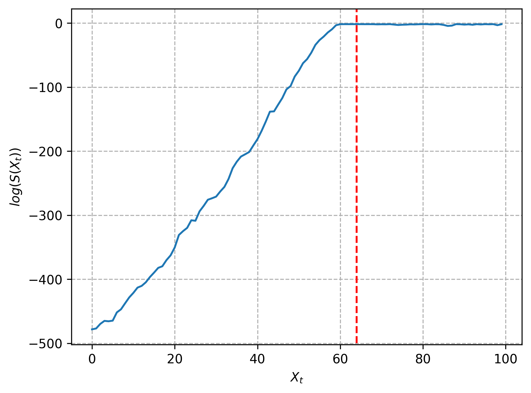
(a) HMC

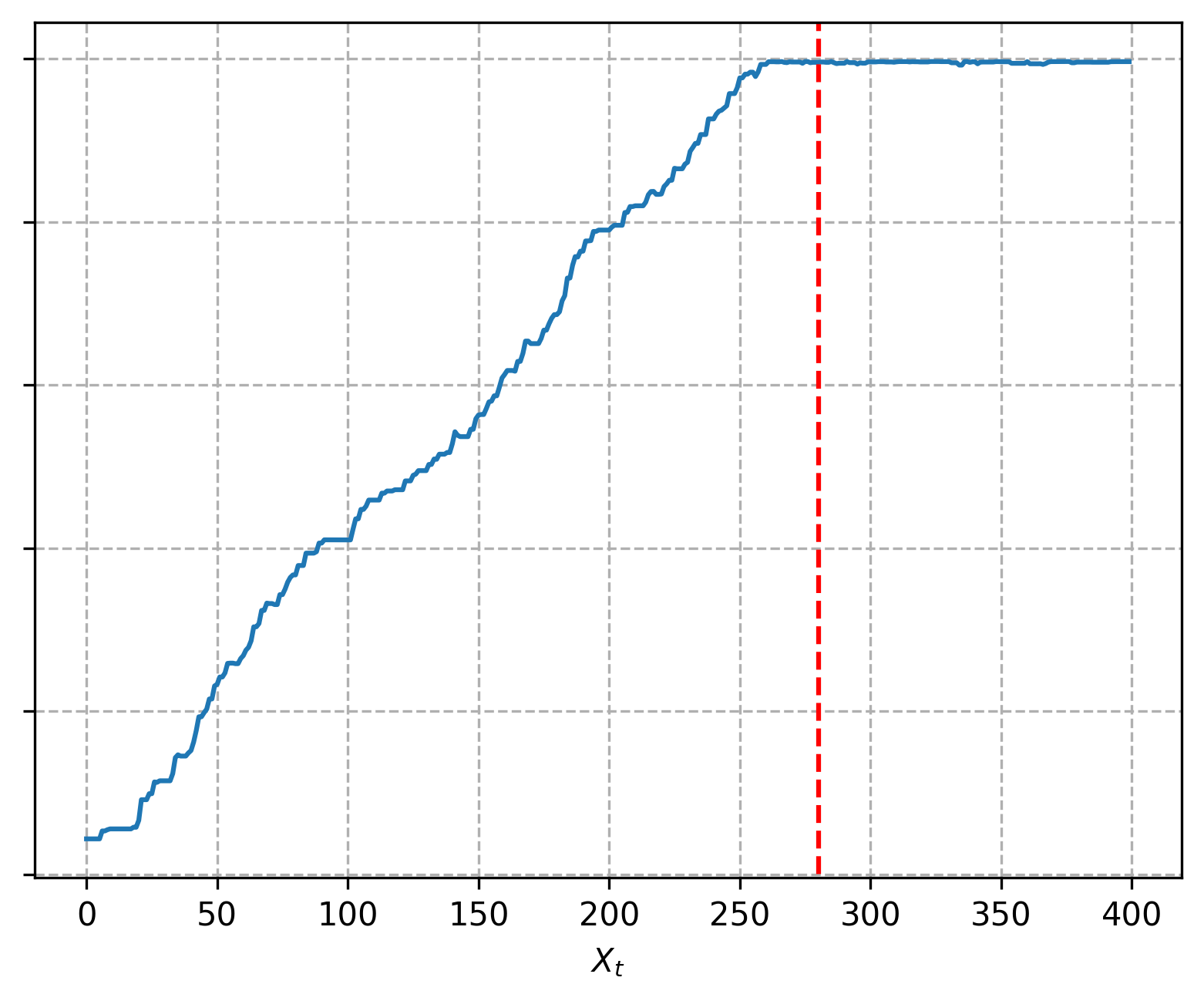
(b) RWMH

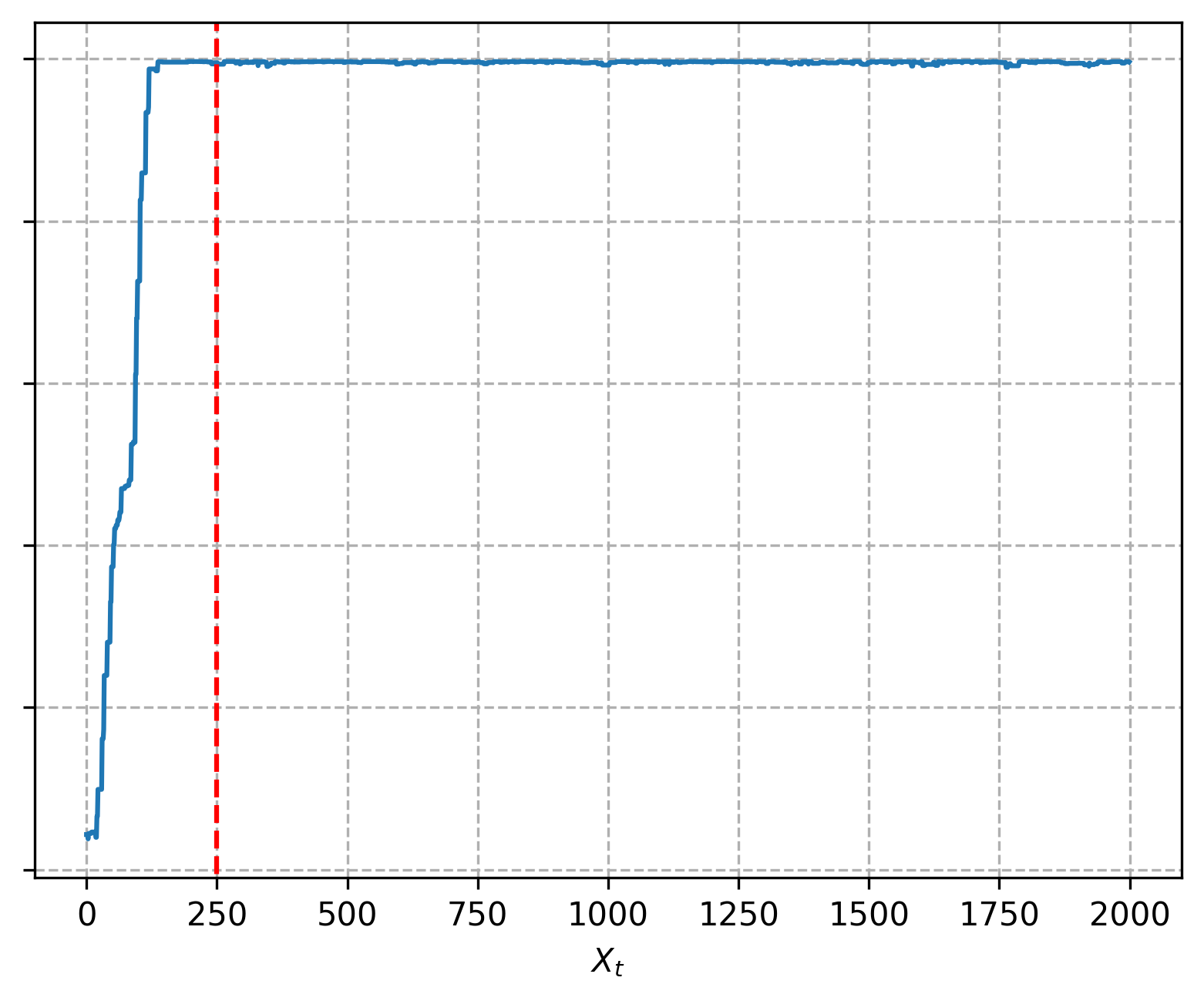
(c) t-walk

Figure 1: Burn-in selection through the log-densities of the states of the Markov chain, the red dashed line represents the length of the chain at which the log-densities stop having increasing behavior.

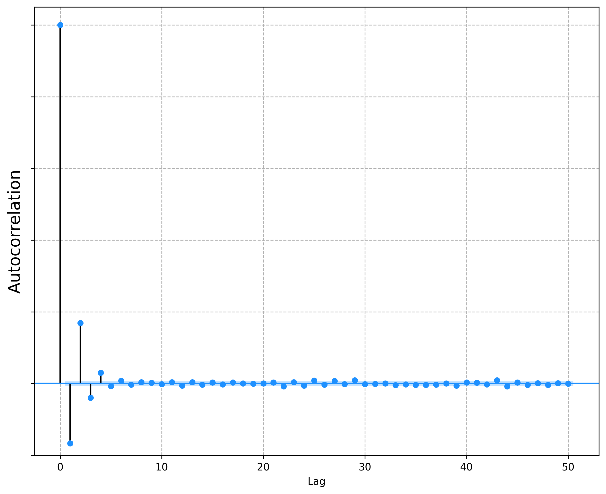
(a) HMC

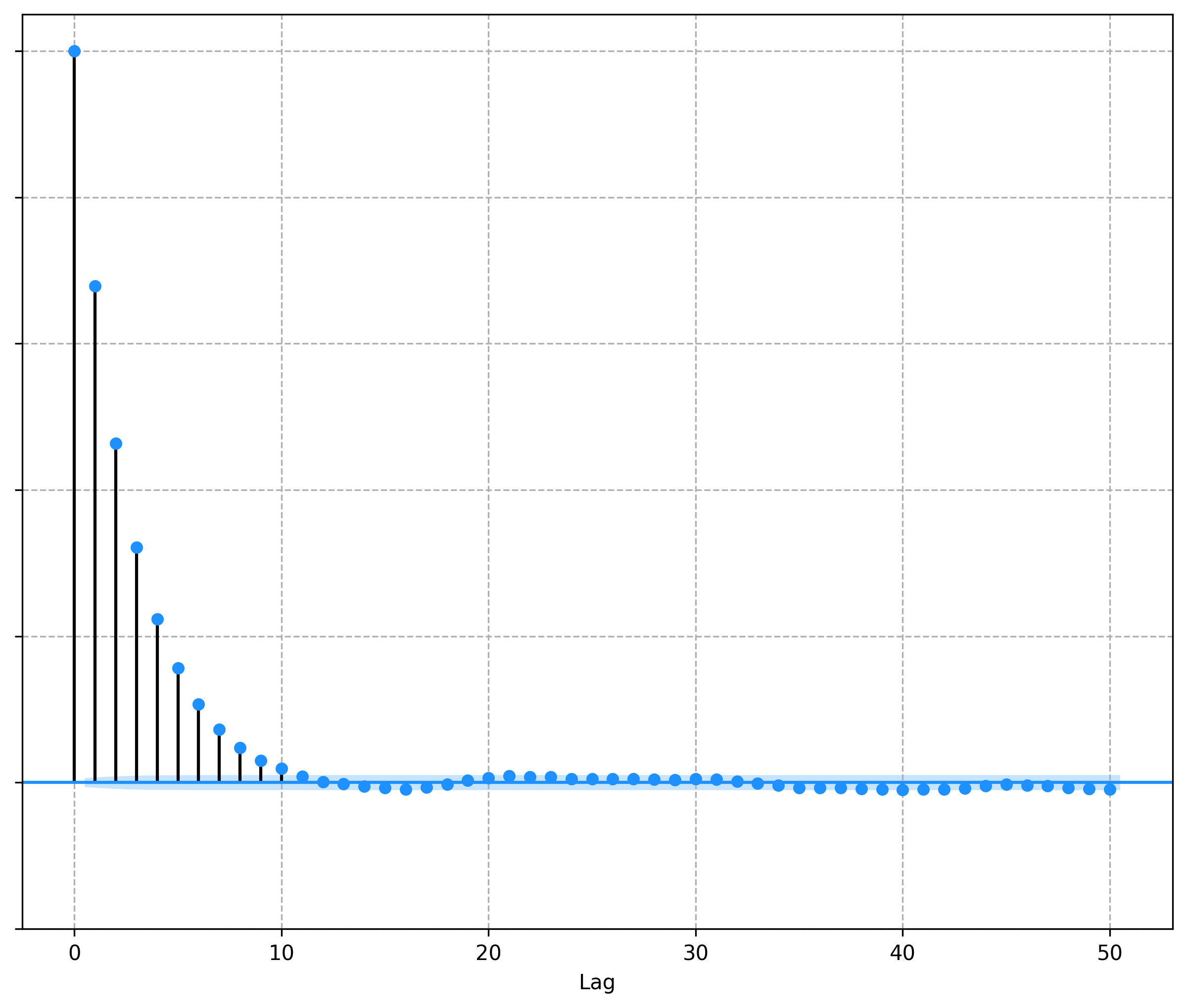
(b) RWMH

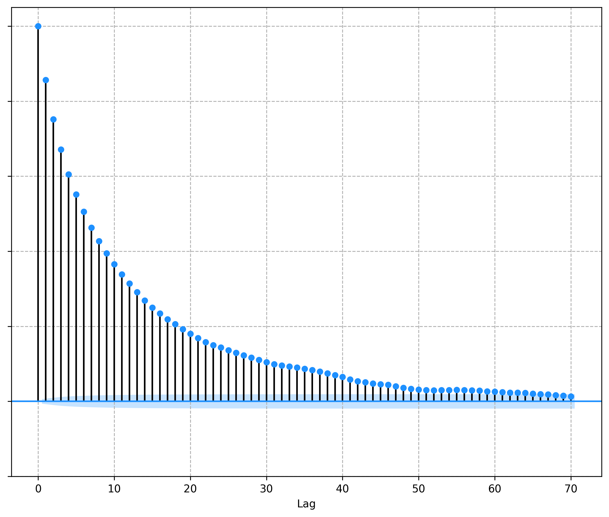
(c) t-walk

Figure 2: Autocorrelations in the Markov chains.

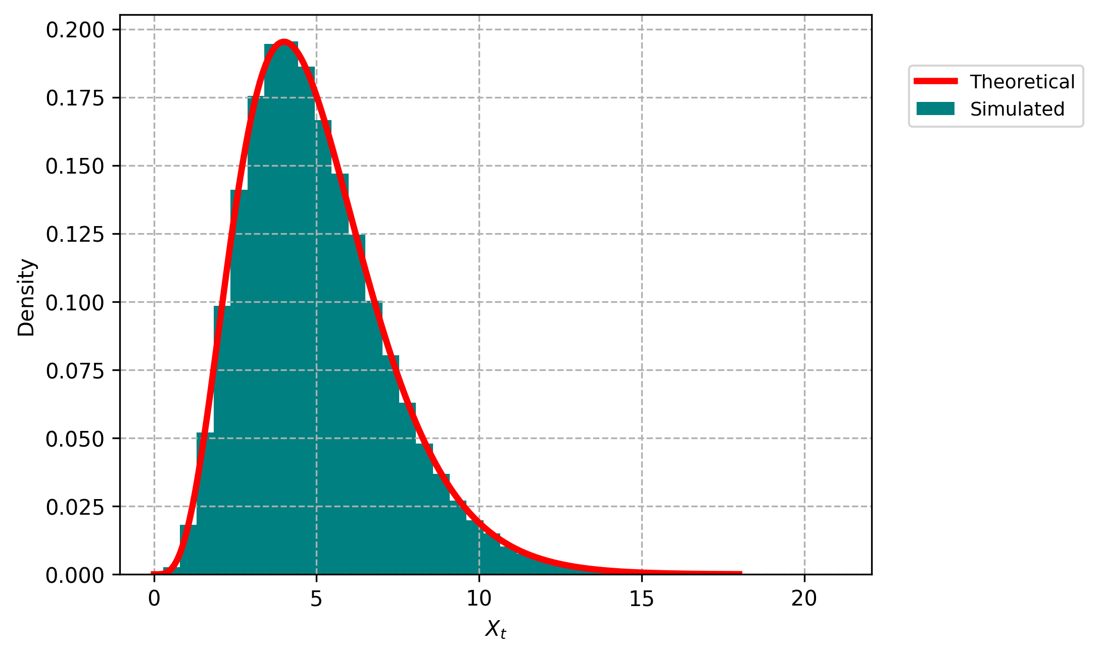
Figure 3: Markov chain density generated with HMC, considering burn-in and lag.

Table 2 shows the main differences when simulating the $Gamma(5,1)$ distribution with the HMC, RWMH and t-walk. As can be seen, the HMC algorithm presents better results since, from the chain of 100,000 states, 99,934 were used as samples of the target distribution, while in RWMH, only 16,620 and with t-walk 4,337. Although the HMC algorithm took longer to execute, it is faster because it generated approximately 2,272 samples per second, while RWMH generated 1,578 and t-walk 804.

Table 2: Comparison between HMC, optimized RWMH and t-walk when simulating from Gamma(5,1) distribution.

	HMC	RWMH	t-walk
Burn-in	65	280	250
IAT	0.9818	5.2574	22.596
Acceptance rate	99.96%	44.03%	59.84%
Efective sample	99,935	16,620	4,337
Execution time (s)	43.99	10.53	5.3927
Seconds per sample (s)	0.0004	0.0006	0.0012

The Python code for this example can be found in link.

4.2 Bivariate normal distribution

In order to facilitate a comparative analysis of the behaviour exhibited by a Markov chain when subjected to the HMC, RWMH and t-walk, a Markov chain was simulated with a bivariate normal distribution designated as the target distribution, with a vector of means $\mu=\left(0,0\right)$ and a variances and covariances matrix

$$\Sigma=\begin{pmatrix}1&-0.85\\ -0.85&1\end{pmatrix},$$ (36)

wich kernel is given by

$$S\left(q\right)=\exp\left(-\frac{q^{T}\Sigma^{-1}q}{2}\right).$$ (37)

To simulate this distribution with the HMC algorithm, we have to define the potential energy of the Hamiltonian as

$$U\left(q\right) = -\log\left(S\left(q\right)\right)$$ (38)

$$= -\log\left(\exp\left(-\frac{q^{T}\Sigma^{-1}q}{2}\right)\right)$$

$$= \frac{q^{T}\Sigma^{-1}q}{2}.$$

Moreover, note that

$$\frac{\partial U}{\partial q}=\Sigma^{-1}q,$$ (39)

this equality is proved in [29].

In this example, the functions (38) and (39) have been employed to implement the HMC algorithm, with $\epsilon=0.15$ and $L=35$ as calibration parameters. In RWMH, a multivariate normal distribution $N(\mu,I_{2}\sigma^{2})$, with $\mu=\left(0,0\right)$ and $\sigma^{2}=0.15^{2}$, was selected as the proposal distribution for the new states in the random walk. Additionally, a lag of 35 was applied to ensure that the length of the chain trajectory was comparable to that of HMC. For both methods, $q=\left(-7,-7\right)$ was taken as the initial point. In the case of the t-walk algorithm, we used starting points $\left(-7,-7\right)$ and $\left(-6.5,-6.5\right)$ to be closer to the starting points of HMC and RWMH. Similarly, in this case we used a lag of 35 to make the computational cost more comparable to the HMC and RWMH.

Graph 4 depicts the trajectories of the chains generated with HMC, RWMH, and t-walk. As can be observed, the initial transitions of the chains generated with HMC and t-walk proceed directly to the region with the highest associated density. In contrast, due to the random nature of RWMH, it is not possible to discern a similar behaviour that would lead the chain to the region of interest. On the other hand, with HMC and t-walk, it is possible to explore a large part of the zone with high density, while the chain generated with RWMH does not seem to have traveled through it. The acceptance rate of the three methods for this simulation is shown in Table 3.

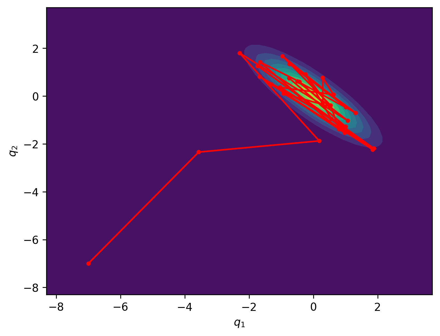
(a) HMC

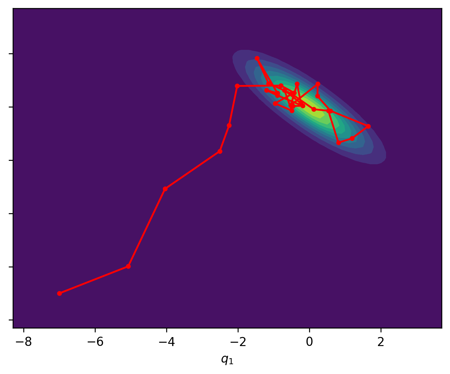
(b) RWMH

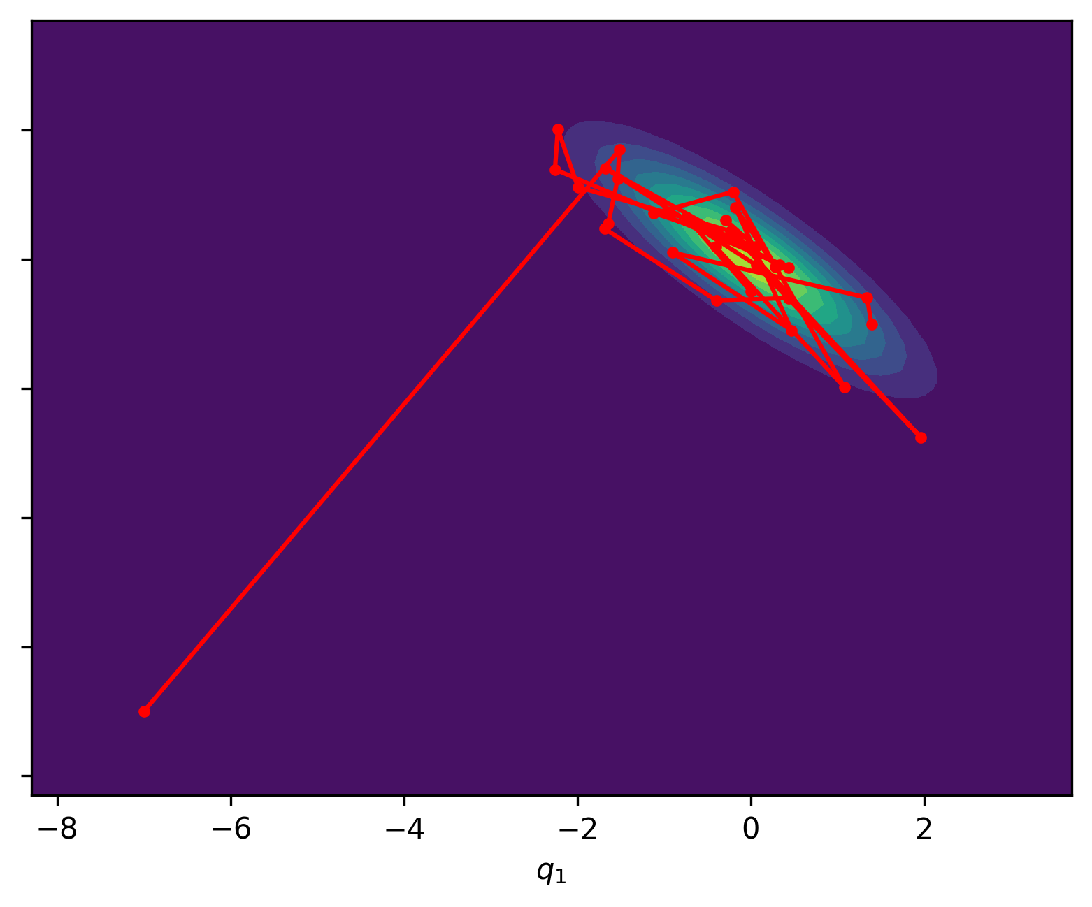
(c) t-walk

Figure 4: Trajectories of the simulated Markov chains.

Table 3: Acceptance rate of HMC, RWMH and t-walk algorithms when simulating from the bivariate normal distribution.

HMC	RWMH	t-walk
100%	83%	42%

The Python code for this example can be found in this link.

4.3 Gaussian mixture

It is known that RWMH presents difficulties when simulating multimodal distributions. In order to show whether HMC or t-walk share this same limitation, in this section, we will simulate a Markov Chain, considering as the target distribution the Gaussian mixture with density

$$S\left(q\right)=0.4f\left(x\mid\mu_{1},\Sigma_{1}\right)+0.6f\left(x\mid\mu_{2},\Sigma_{2}\right),$$ (40)

where $f$ is the density function of the multivariate normal distribution given in (43) and

$$\mu_{1} = \left(-4,-4\right),\hskip 28.45274pt\Sigma_{1}=\begin{pmatrix}1&0.5\\ 0.5&1\end{pmatrix},$$ (41)

$$\vskip 28.45274pt\mu_{2} = \left(5,5\right),\hskip 42.67912pt\Sigma_{2}=\begin{pmatrix}1&-0.3\\ -0.3&1\end{pmatrix}.$$ (42)

$$f\left(x\mid\mu,\Sigma\right)=\frac{1}{\left(2\pi\right)^{\frac{n}{2}}\det\left(\Sigma\right)^{\frac{1}{2}}}\exp\left(-\frac{1}{2}\left(x-\mu\right)^{t}\sideset{}{{}^{-1}}{\sum}\left(x-\mu\right)\right).$$ (43)

To simulate this distribution using the HMC algorithm, we must define the potential energy $U$ as

$$U\left(q\right) = -\log\left(0.4f\left(q\mid\mu_{1},\Sigma_{1}\right)+0.6f\left(q\mid\mu_{2},\Sigma_{2}\right)\right).$$ (44)

Note also that

$$\frac{\partial U}{\partial q} = \frac{\partial}{\partial q}\left(-\log\left(0.4f\left(q\mid\mu_{1},\Sigma_{1}\right)+0.6f\left(q\mid\mu_{2},\Sigma_{2}\right)\right)\right)$$ (45)

$$= -\frac{0.4\frac{\partial}{\partial q}f\left(q\mid\mu_{1},\Sigma_{1}\right)+0.6\frac{\partial}{\partial q}f\left(q\mid\mu_{2},\Sigma_{2}\right)}{0.4f\left(q\mid\mu_{1},\Sigma_{1}\right)+0.6f\left(q\mid\mu_{2},\Sigma_{2}\right)}.$$

In [29] it is proved that

$$\frac{\partial}{\partial q}f\left(q\mid\mu,\Sigma\right)=f\left(q\mid\mu,\Sigma\right)\Sigma^{-1}\left(q-\mu\right),$$

so (45) can be rewritten as

$$\frac{\partial U}{\partial q}=-\frac{0.4f\left(q\mid\mu_{1},\Sigma_{1}\right)\Sigma_{1}^{-1}\left(q-\mu_{1}\right)+0.6f\left(q\mid\mu_{2},\Sigma_{2}\right)\Sigma_{2}^{-1}\left(q-\mu_{2}\right)}{0.4f\left(q\mid\mu_{1},\Sigma_{1}\right)+0.6f\left(q\mid\mu_{2},\Sigma_{2}\right)}.$$ (46)

In this example, to generate the simulations with the HMC algorithm the functions (44) and (46) are required. In addition, we used as calibration parameters $\epsilon=0.2$ and $L=30$. In RWMH, a multivariate normal distribution $N(\mu,I_{2}\sigma^{2})$ was used for the proposed random walk, with $\mu=\left(0,0\right)$ and $\sigma^{2}=0.2^{2}$, and a lag of 30 was applied to make the chain length comparable to that of HMC. We executed HMC and RWMH twice one considering the initial point $\left(-9,-9\right)$ and the other $\left(2.5,2,5\right)$. In the case of t-walk we used as initial points $\left(-9,-9\right)$ and $\left(-8,-8\right)$ for the first execution and $\left(2.5,2.5\right)$ and $\left(3.5,3.5\right)$ for the second, moreover we also used a lag $l=30$ to make more comparable with the number of iterations of RWMH. In each execution we generated chains of 5,000 states.

The simulations obtained in this example are illustrated in Image 5. As can be observed, the t-walk algorithm was the only one capable of adequately simulating the bimodal distribution due to its four movements. In contrast, the trajectories of HMC and RWMH exhibited a propensity to become trapped within a distribution mode dependent on the initial point employed.

It is established that certain MCMC methods encounter difficulties when simulating multimodal distributions. Nevertheless, it is feasible to simulate such distributions using these methods. The article [25] proposes potential solutions for the practical simulation of multimodal distributions using MCMC methods.

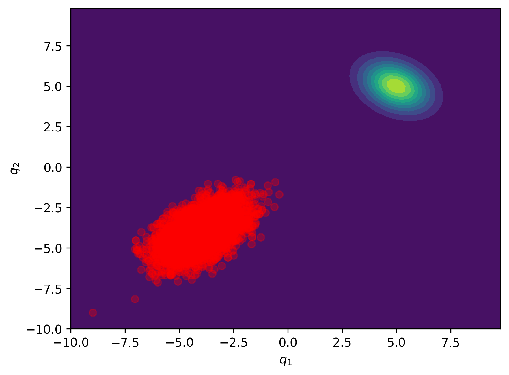
(a) HMC

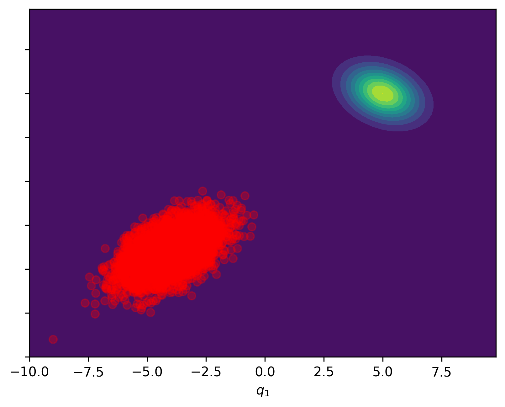
(b) RWMH

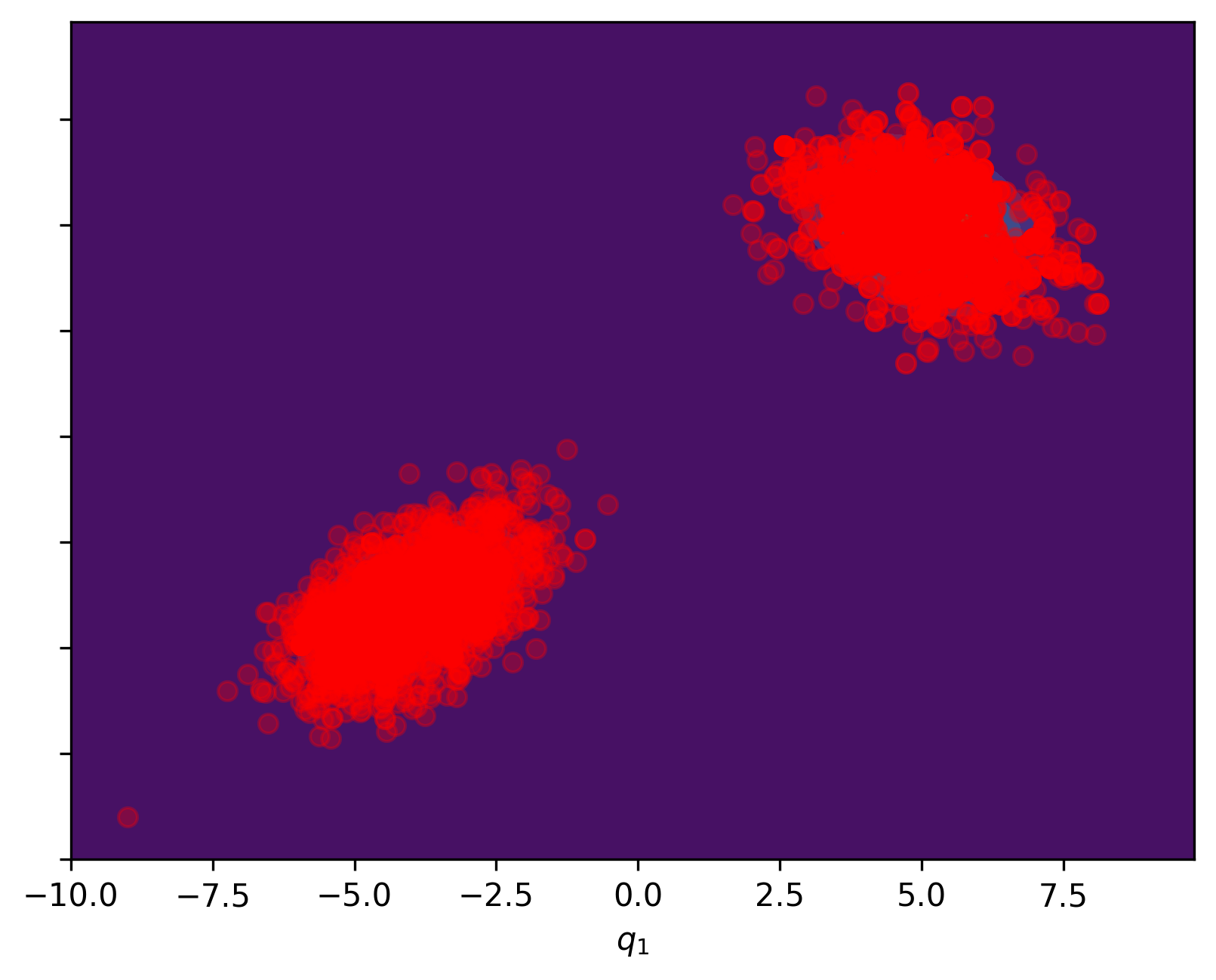
(c) t-walk

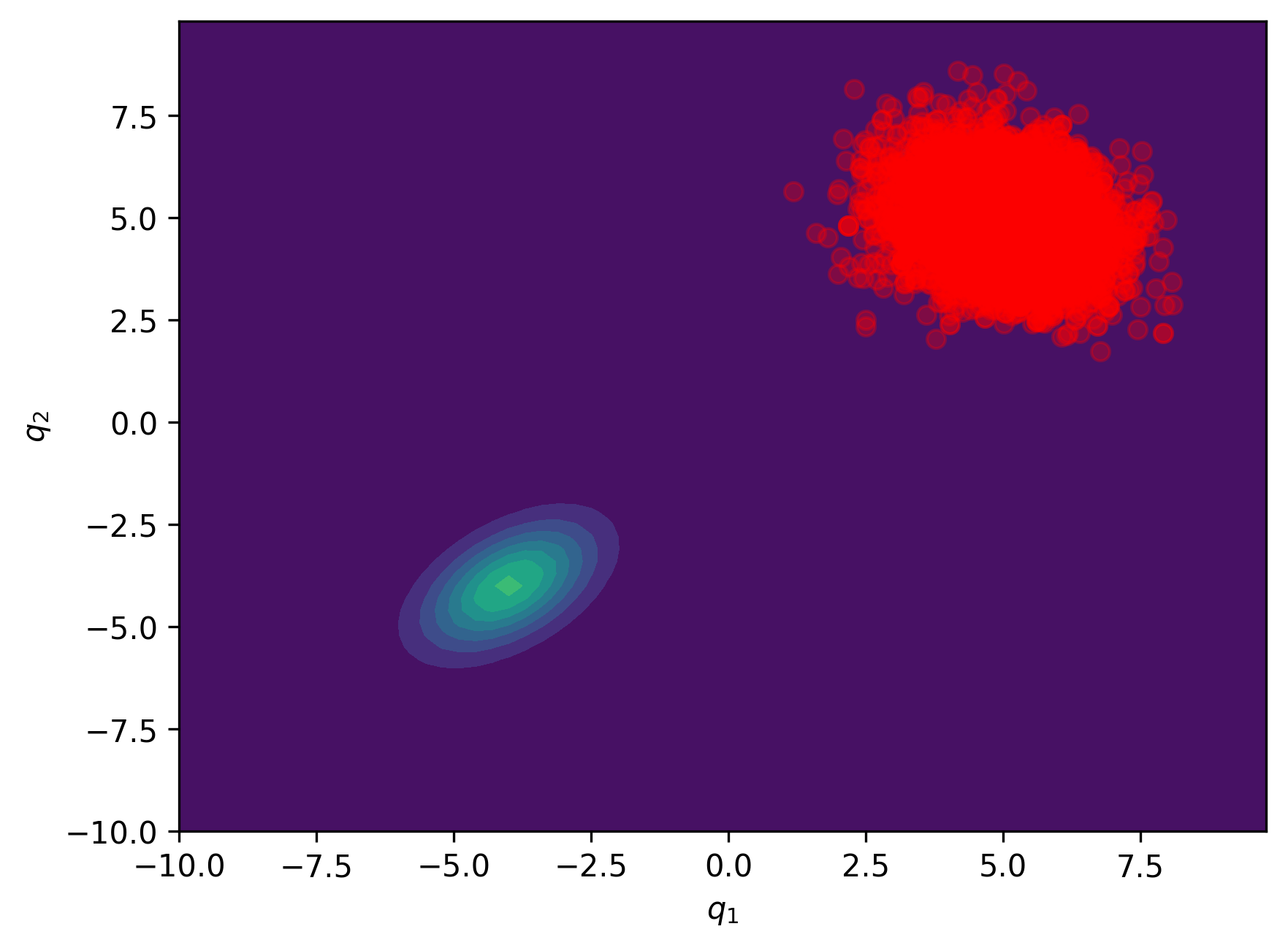
(d) HMC

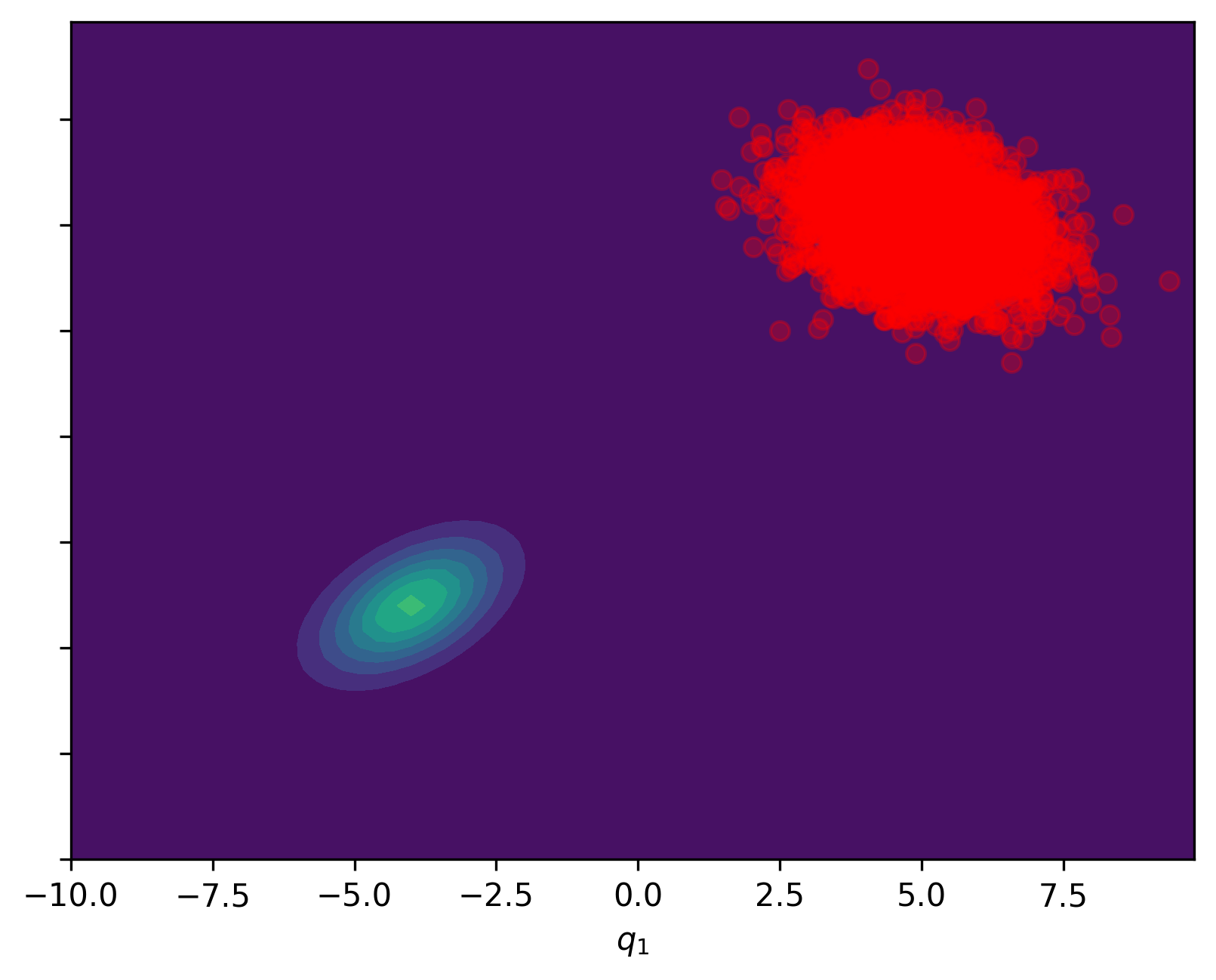
(e) RWMH

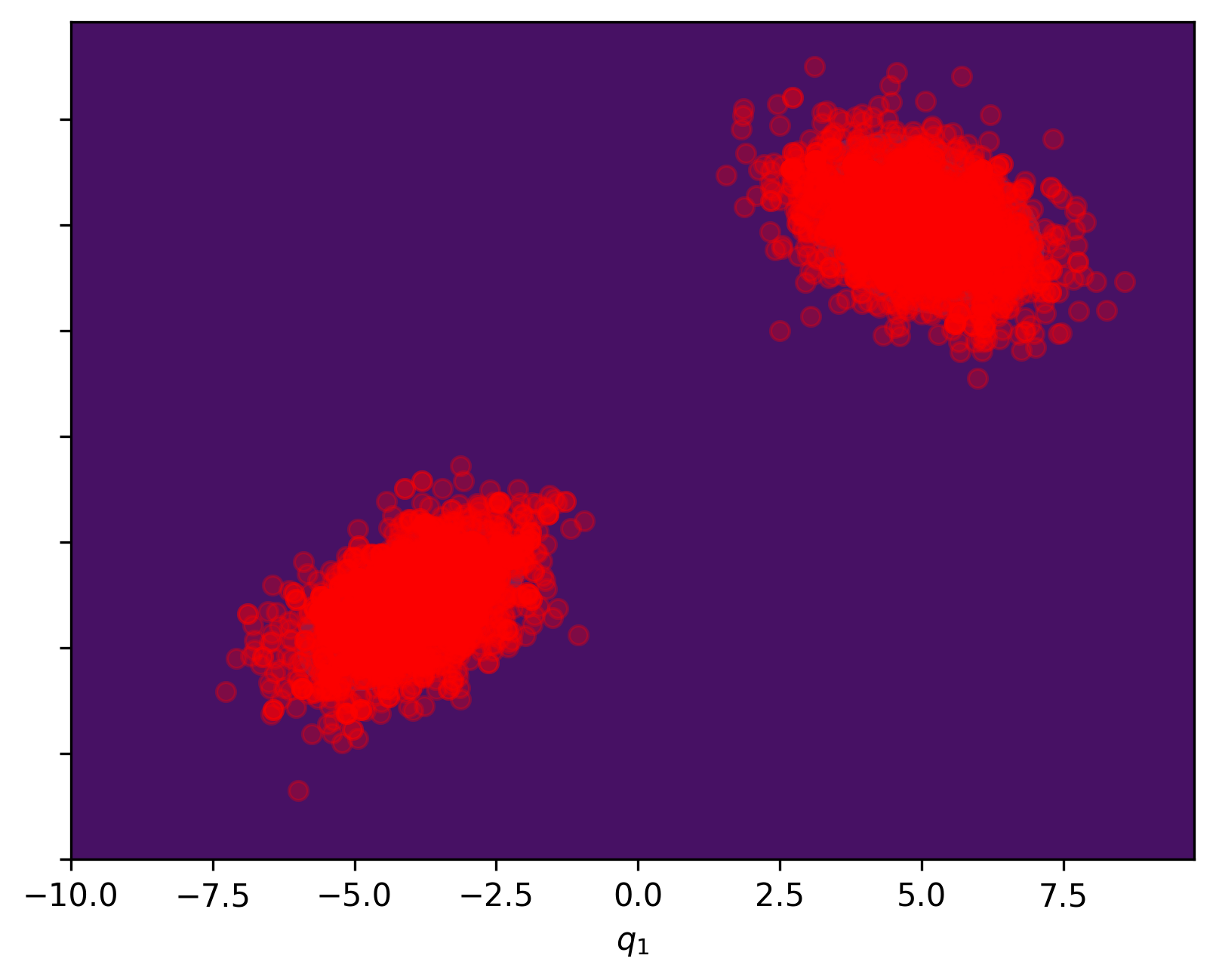
(f) t-walk

Figure 5: Simulation of Gaussian mixture: for (a) and (b), (-9, -9) was taken as the starting point; for (c), (-9, -9) and (-8, -8); for (d) and (e), (2.5, 2.5); and for (f), (2.5, 2.5) and (3.5, 3.5).

Tables 4 and 5 illustrate the execution time and acceptance rate of the algorithms employed to simulate the chains in this example. It can be observed that, irrespective of the initial condition, HMC exhibits the highest acceptance rate and is more rapid than RWMH. Nevertheless, in this specific instance, it is not an optimal choice to utilise HMC, as it will not yield an accurate simulation of the target distribution.

Table 4: Execution times and acceptance rates of the Markov chain simulations with starting points $(-9,-9)$ for HMC and RWMH, and $(-9,-9)$, $(-8,-8)$ for t-walk.

	HMC	RWMH	t-walk
Acceptance rate	93.9% s	88.9%	17.1%
Execution time (s)	115.8	171.4	119.8

Table 5: Execution times and acceptance rates of the Markov chain simulations with starting points $(2.5,2.5)$ for HMC and RWMH, and $(2.5,2.5)$, $(3.5,3.5)$ for t-walk.

	HMC	RWMH	t-walk
Acceptance rate	91.5%	90.0%	29.5%
Execution time (s)	120.7	170.5	109.2

The Python code for this example can be found in this link.

4.4 Hierarchical Normal model (Eight Schools model)

The example of the eight schools is a Bayesian model presented in [14], where the effect of eight schools’ training programmes for the SAT (Scholastic Aptitude Test) is studied. This test is used by universities in the USA as a means of assessing the aptitude of applicants, with the objective of making informed decisions regarding their admission. The SAT is designed to reflect the knowledge acquired over several years of education; therefore, it is anticipated that late efforts to enhance test scores will be ineffective. The objective of the eight-school model is to ascertain the impact of the training programmes on the test scores. Table 6 presents the estimated difference in test scores between students who participated in the training programme and those who did not, along with the respective sample deviations.

Table 6: Training effects on SAT and their sample deviation. The data were obtained from [26].

School	Effect $y_{i}$	Sample standard
		deviation $\kappa_{i}^{2}$
1	2.8	0.8
2	0.8	0.5
3	-0.3	0.8
4	0.7	0.6
5	-0.1	0.5
6	0.1	0.6
7	1.8	0.5
8	1.2	0.4

For the purposes of modeling, the proposed framework assumes that the training impact of the schools, $y_{i}\mid\theta_{i},\kappa_{i}$, is conditionally independent and satisfies

$$y_{i}\mid\theta_{i},\kappa_{i}\sim N\left(\theta_{i},\kappa^{2}\right)\text{ for i$\in\left\{1,2,...,8\right\}$},$$ (47)

where $\kappa_{i}$ is known and is given by the sample deviation of the $i$-th school presented in table 6, and

$$\theta_{i}=\mu+\tau\eta_{i}.$$ (48)

In this exercise, we will make inferences on the parameters $\mu,\tau\text{ and }\eta_{i}$ with $i\in\left\{1,2,...,8\right\}$, following the approach presented in the paper [26], where independent distributions $N(0,1)$ are assigned as the a priori distributions for the variables $\mu,\tau\text{ and }\eta_{i}$ such that the a priori join density $p$ satisfies that

$$p\left(\eta,\mu,\tau\right)\propto\exp\left(-\frac{\mu^{2}}{2}\right)\exp\left(-\frac{\tau^{2}}{2}\right)\stackrel{{\scriptstyle[}}{{i}}=1]{8}{\prod}\exp\left(-\frac{\eta_{i}^{2}}{2}\right),$$ (49)

where $\eta=\left(\eta_{1},\eta_{2},...,\eta_{8}\right)$.

Note that the likelihood, $\mathcal{L}\left(y\mid\eta,\mu,\tau\right)$, satisfies that

$$\mathcal{L}\left(y\mid\eta,\mu,\tau\right)\propto\stackrel{{\scriptstyle[}}{{i}}=1]{8}{\prod}\exp\left(-\frac{\left(y_{i}-\left(\mu+\tau\eta_{i}\right)\right)^{2}}{2\kappa_{i}^{2}}\right),$$ (50)

and the posterior density is given by

$$S^{\prime}\left(y\mid\eta,\mu,\tau\right)=\frac{p\left(\eta,\mu,\tau\right)\mathcal{L}\left(y\mid\eta,\mu,\tau\right)}{\int_{(\eta,\mu,\tau)\in\mathbb{R}^{10}}\mathcal{L}\left(y\mid\eta,\mu,\tau\right)p\left(\eta,\mu,\tau\right)d\eta d\mu d\tau}.$$ (51)

Substituting (49) and (50) in (51), we can observe that the posterior density is proportional to the function

In order to simulate the posterior distribution using HMC, the potential energy of the Hamiltonian is defined as

$$U=-\log\left(S\left(y\mid\eta,\mu,\tau\right)\right)=\frac{\mu^{2}}{2}+\frac{\tau^{2}}{2}+\sum_{i=1}^{8}\frac{\eta_{i}^{2}}{2}+\sum_{i=1}^{8}\left(\frac{\left(y_{i}-\left(\mu+\tau\eta_{i}\right)\right)^{2}}{2\kappa_{i}^{2}}\right),$$ (53)

and its gradient vector, $\left(\frac{\partial U}{\partial\eta_{1}},\dots,\frac{\partial U}{\partial\eta_{8}},\frac{\partial U}{\partial\mu},\frac{\partial U}{\partial\tau}\right)$, must be computed, with its entries given by

$$\frac{\partial U}{\partial\eta_{i}} = \eta_{i}-\left(\frac{\left(y_{i}-\left(\mu+\tau\eta_{i}\right)\right)}{\kappa_{i}^{2}}\right)\tau\text{ for i$\in\left\{1,2,...,8\right\}$},$$ (54)

$$\frac{\partial U}{\partial\mu} = \mu-\stackrel{{\scriptstyle[}}{{i}}=1]{8}{\sum}\left(\frac{\left(y_{i}-\left(\mu+\tau\eta_{i}\right)\right)}{\kappa_{i}^{2}}\right),$$ (55)

$$\frac{\partial U}{\partial\tau} = \tau-\stackrel{{\scriptstyle[}}{{i}}=1]{8}{\sum}\left(\frac{\left(y_{i}-\left(\mu+\tau\eta_{i}\right)\right)}{\kappa_{i}^{2}}\right)\eta_{i}.$$ (56)

In this example, a chain of 500,000 was simulated, having (51) as the target density, with the HMC, RWMH, and t-walk methods. To generate the simulation with the HMC method, the gradient $\left(\frac{\partial U}{\partial\eta_{1}},...,\frac{\partial U}{\partial\eta_{8}},\frac{\partial U}{\partial\mu},\frac{\partial U}{\partial\tau}\right)$ and the function (53) were used as inputs, as initial point we took $\left(2,2,...,2\right)$ and as calibration parameters $\epsilon=0.08$ and $L=60$, which although not selected under an optimality criterion, these were chosen with consideration of a small $\epsilon$ and a large $L$, ensuring adequate transitions in the chain and favourable outcomes.

To simulate the target distribution with RWMH, we used the initial point $\left(2,2,...,2\right)$ arbitrarily, and for the proposals of the new states, a multivariate normal distribution $N(\mu,I_{10}\sigma^{2})$, with $\mu=\left(0,0,...,0\right)$ and $\sigma^{2}=0.32^{2}$, achieving an acceptance rate of 24.6%. The choice of $\sigma^{2}$ was made looking for the acceptance rate to be close to the optimal rate of 23.4% stated in [31].

The t-walk algorithm does not necessitate the calibration of parameters; however, its execution does require the input of two initial points. In this instance, $\left(2,2,...,2\right)$ and $\left(3,3,...,3\right)$ were used.

To visualize the results, we will present the joint densities $\left(\mu,\tau\right)$ and $\left(\tau,\eta_{1}\right)$; for this, it is necessary to determine the burn-in and lag period of the simulated chains. Figure 6 shows the burn-in period of the simulated chains. As can be observed, the chain generated by the HMC is the first to reach zones with high density.

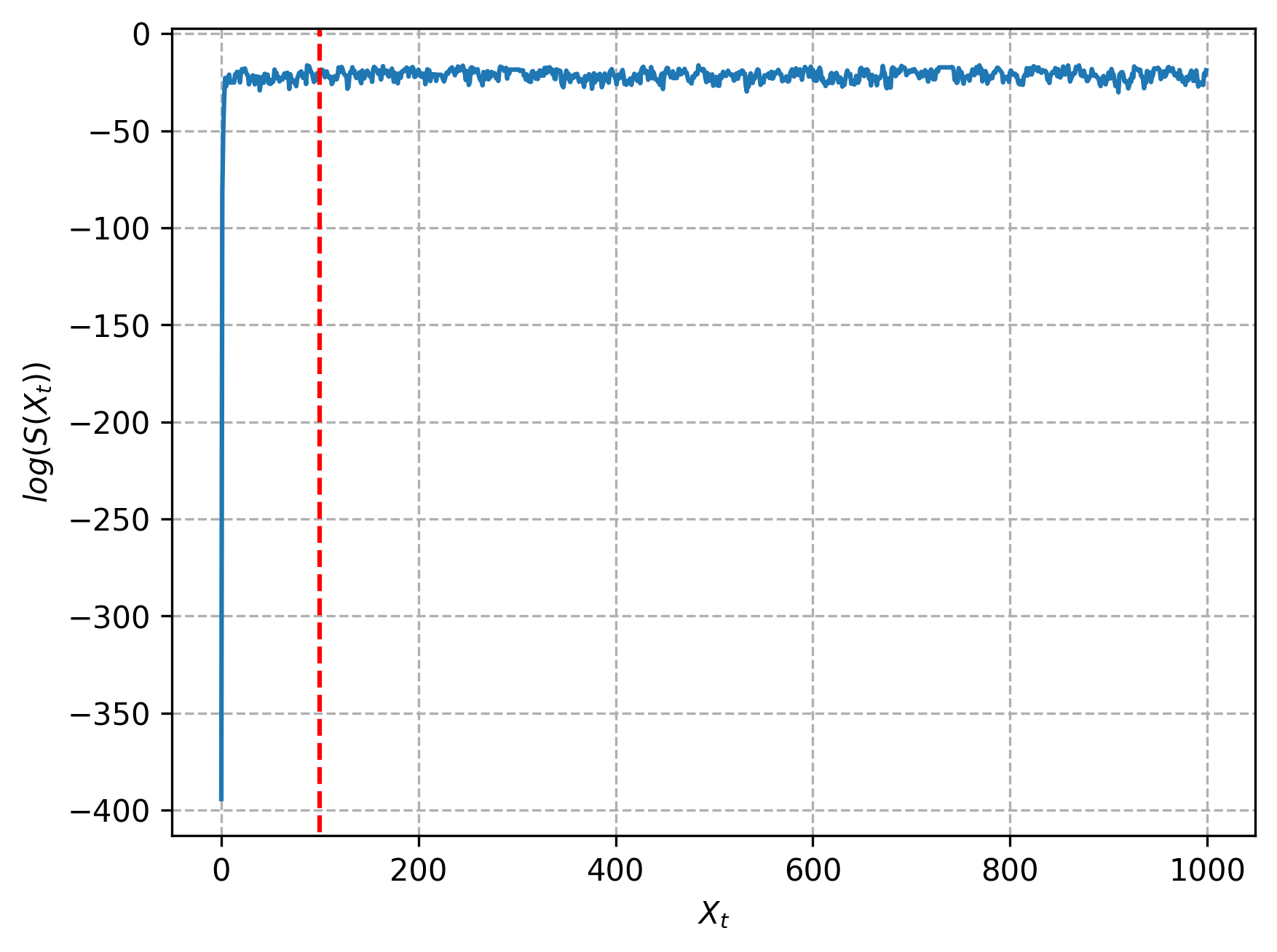
(a) HMC

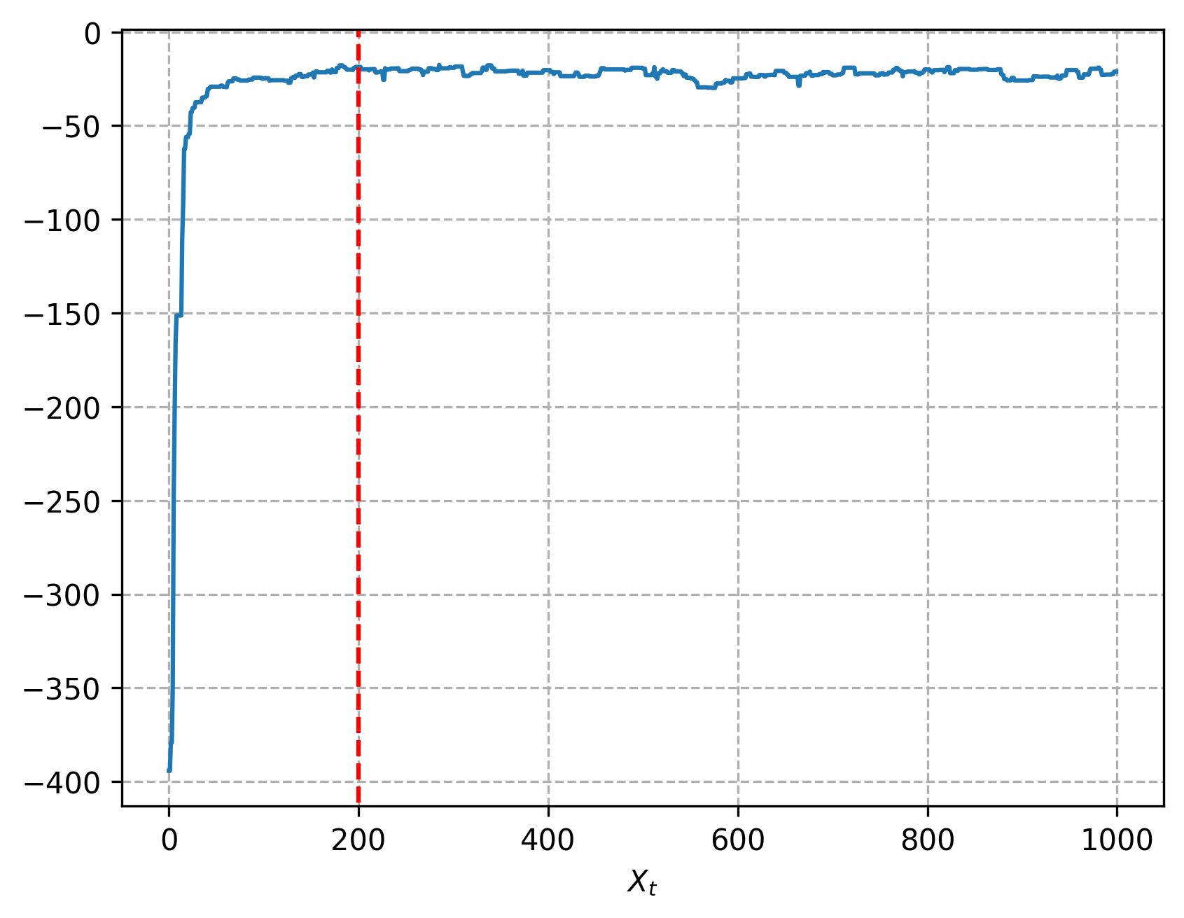
(b) RWMH

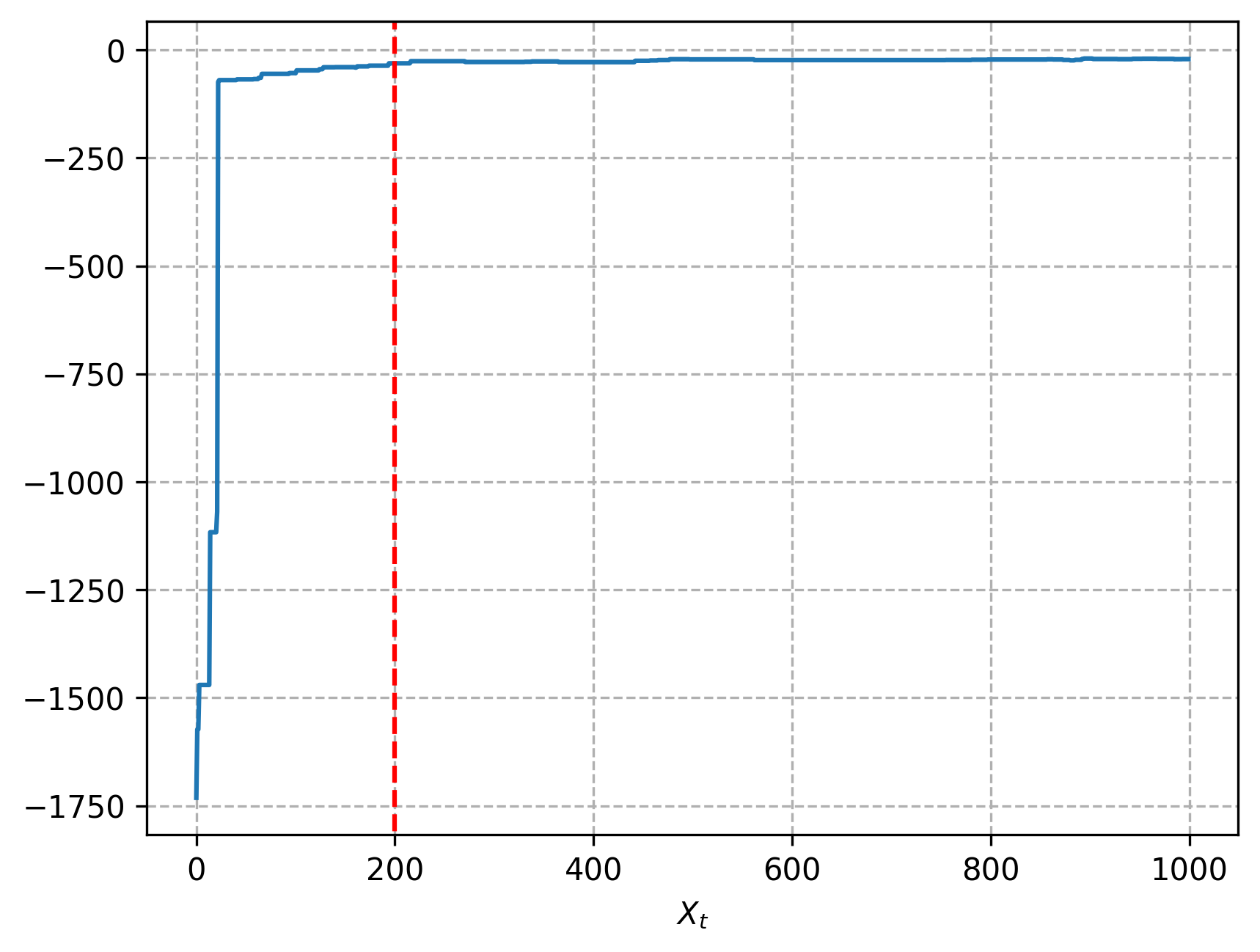
(c) t-walk

Figure 6: Burn-in period in simulated chains with target density $S^{\prime}$. The dashed red line represents the number of chain states at which the log densities cease to have increasing behavior.

In order to select the lag $l$ that would yield pseudo-independent samples of each chain, the autocorrelations of the marginal variables were analysed, and with the three methods, the one with the highest autocorrelation was $\tau$, so $l$ was chosen as the lag in which the autocorrelations of $\tau$ were not statistically significant. Figure 7 shows the autocorrelations of $\tau$, as can be seen, the chain generated with HMC has a lower dependence in the previous states than those of the chains generated by RWMH and t-walk.

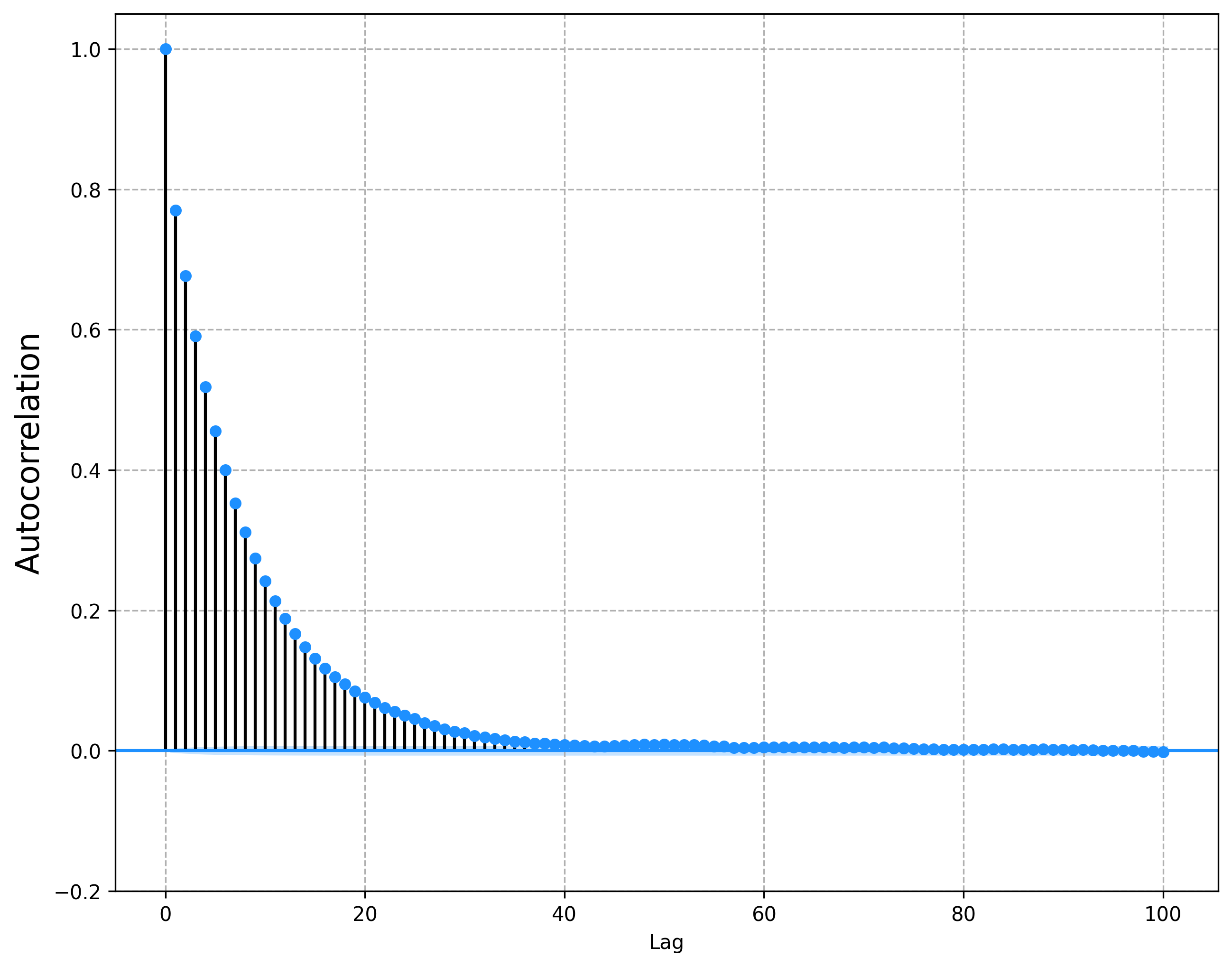
(a) HMC

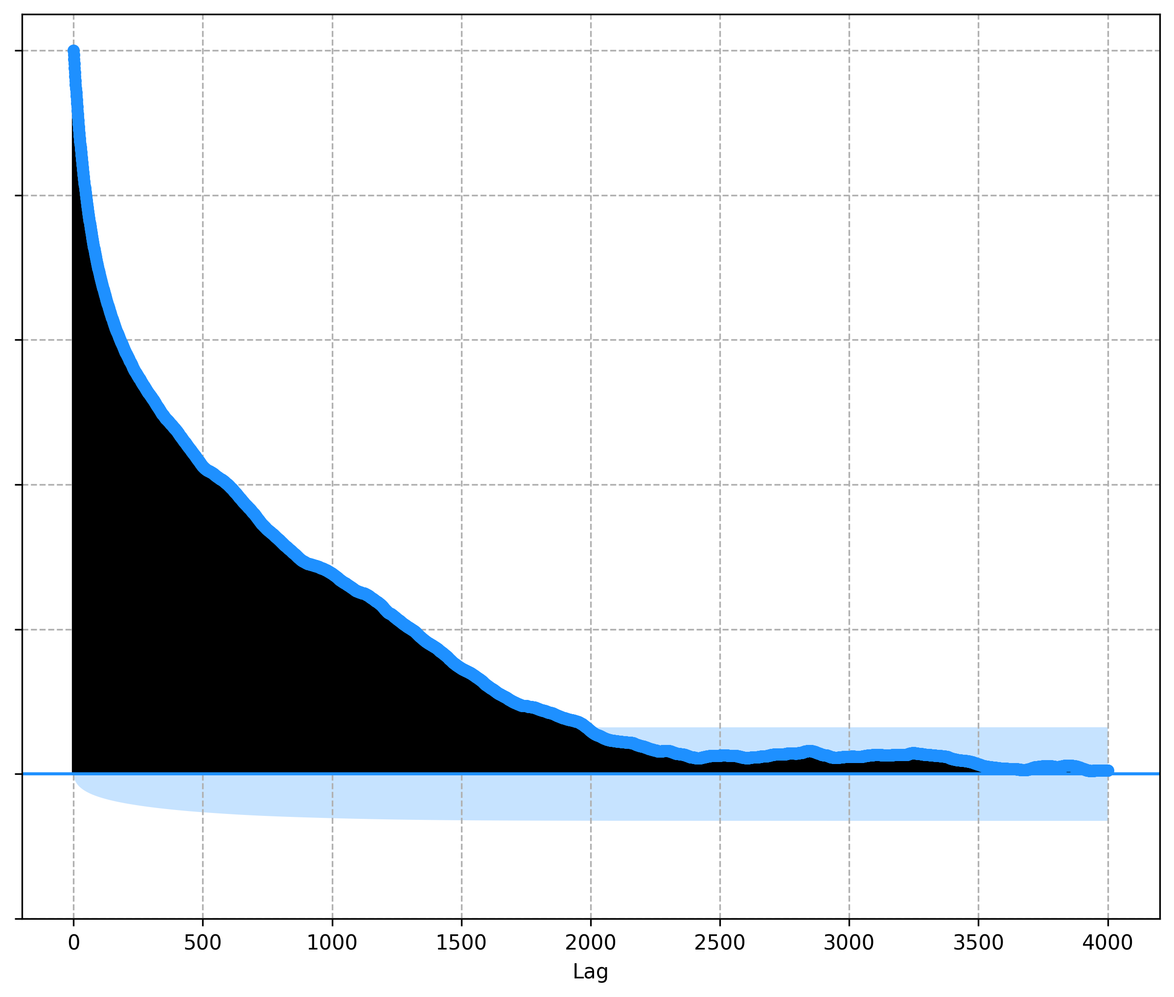
(b) RWMH

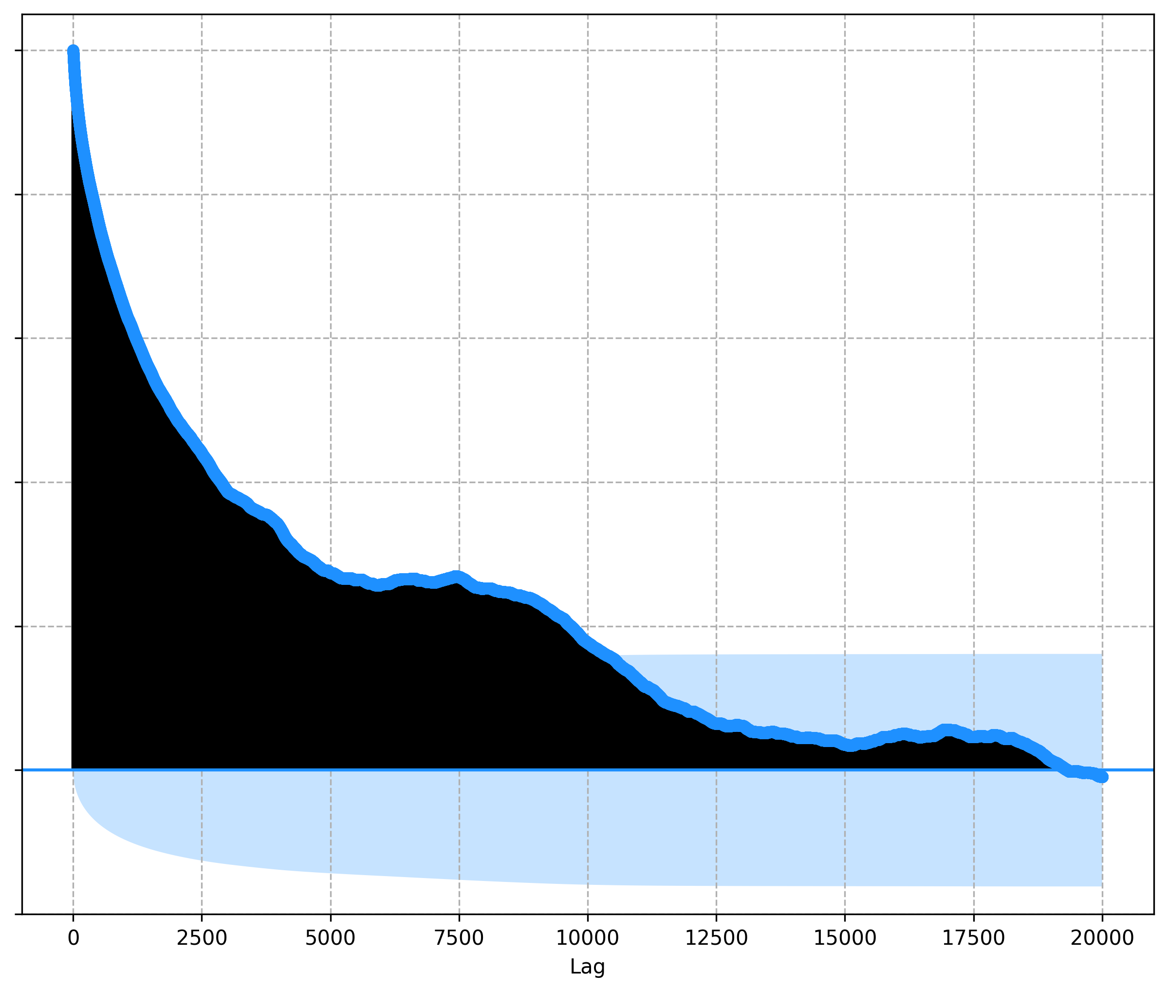
(c) t-walk

Figure 7: Autocorrelations of the marginal distribution of $\tau$ in the simulated chains with target density $S^{\prime}$.

Table 7 illustrates the principal discrepancies between the HMC, RWMH, and t-walk algorithms when simulating the Markov chain with target density $S^{\prime}$. As demonstrated, the HMC is more time-efficient than the RWMH and t-walk, as it requires less time to generate a sample. This is primarily due to the fact that the states of the chains simulated with RWMH and t-walk exhibit a high degree of correlation. Consequently, a significant proportion of the simulations must be discarded in order to obtain a pseudo-independent sample. Figure 8 illustrates the joint densities of the effective sample obtained from the simulated chains with HMC, RWMH, and t-walk.

HMC

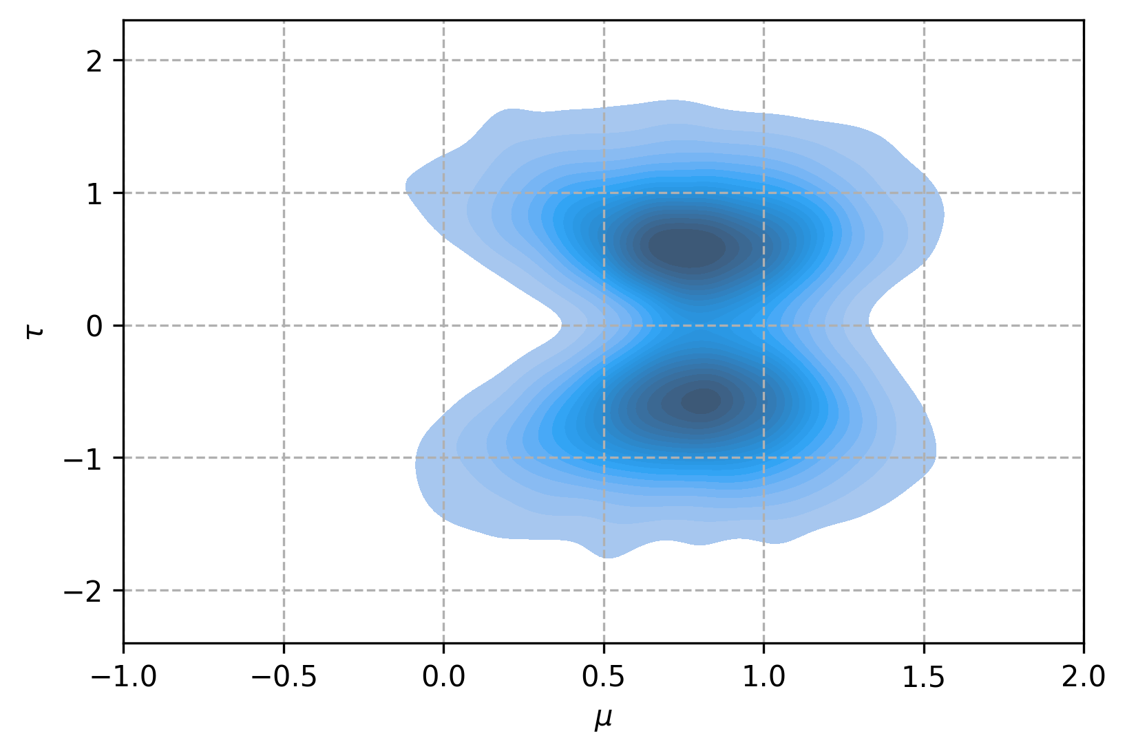
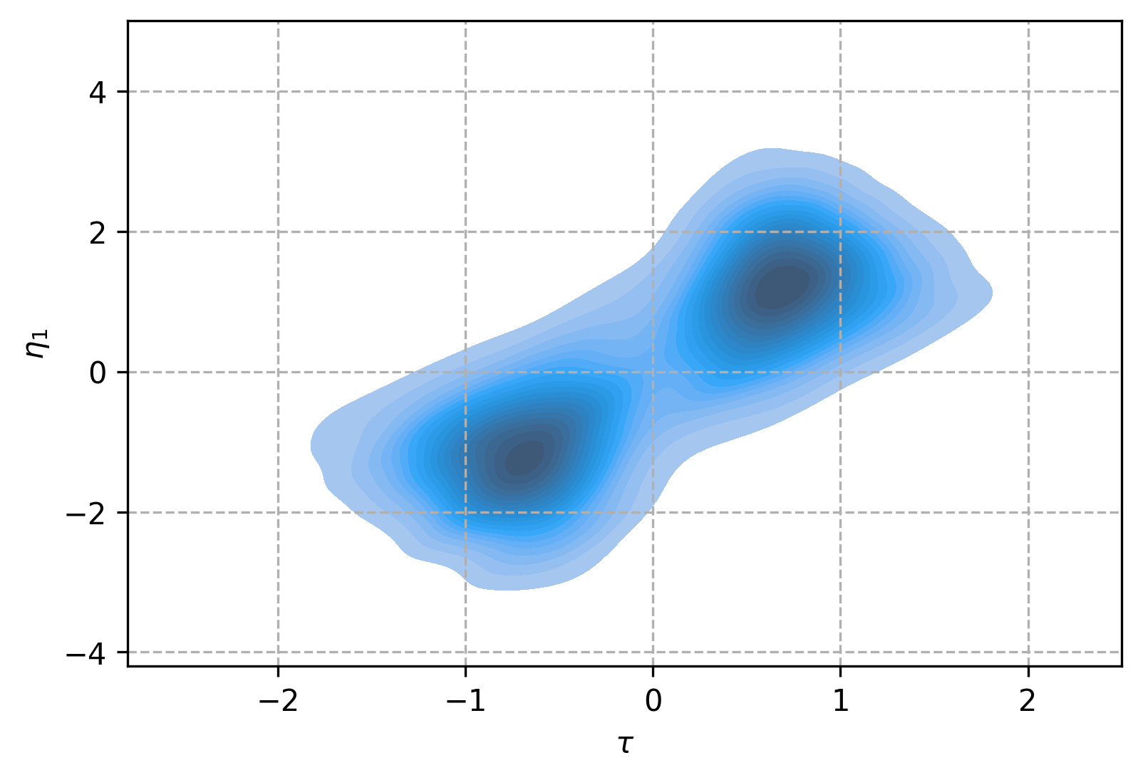
RWMH

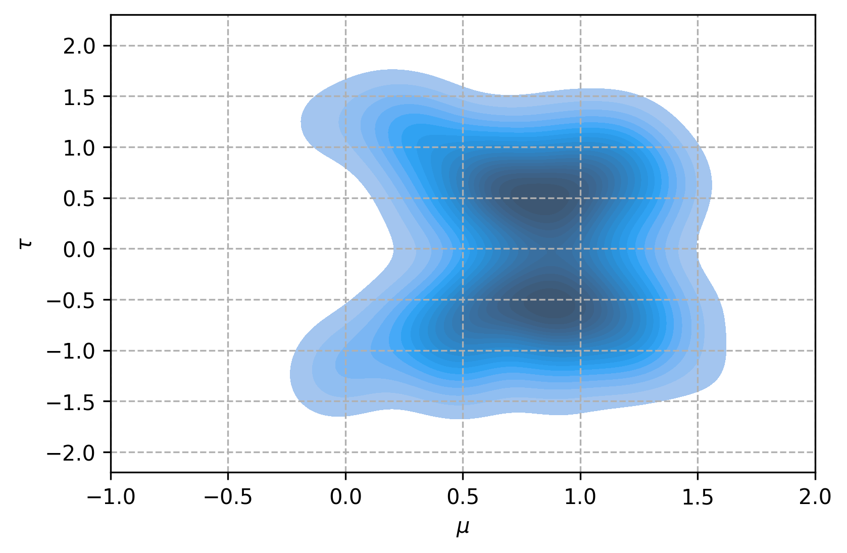
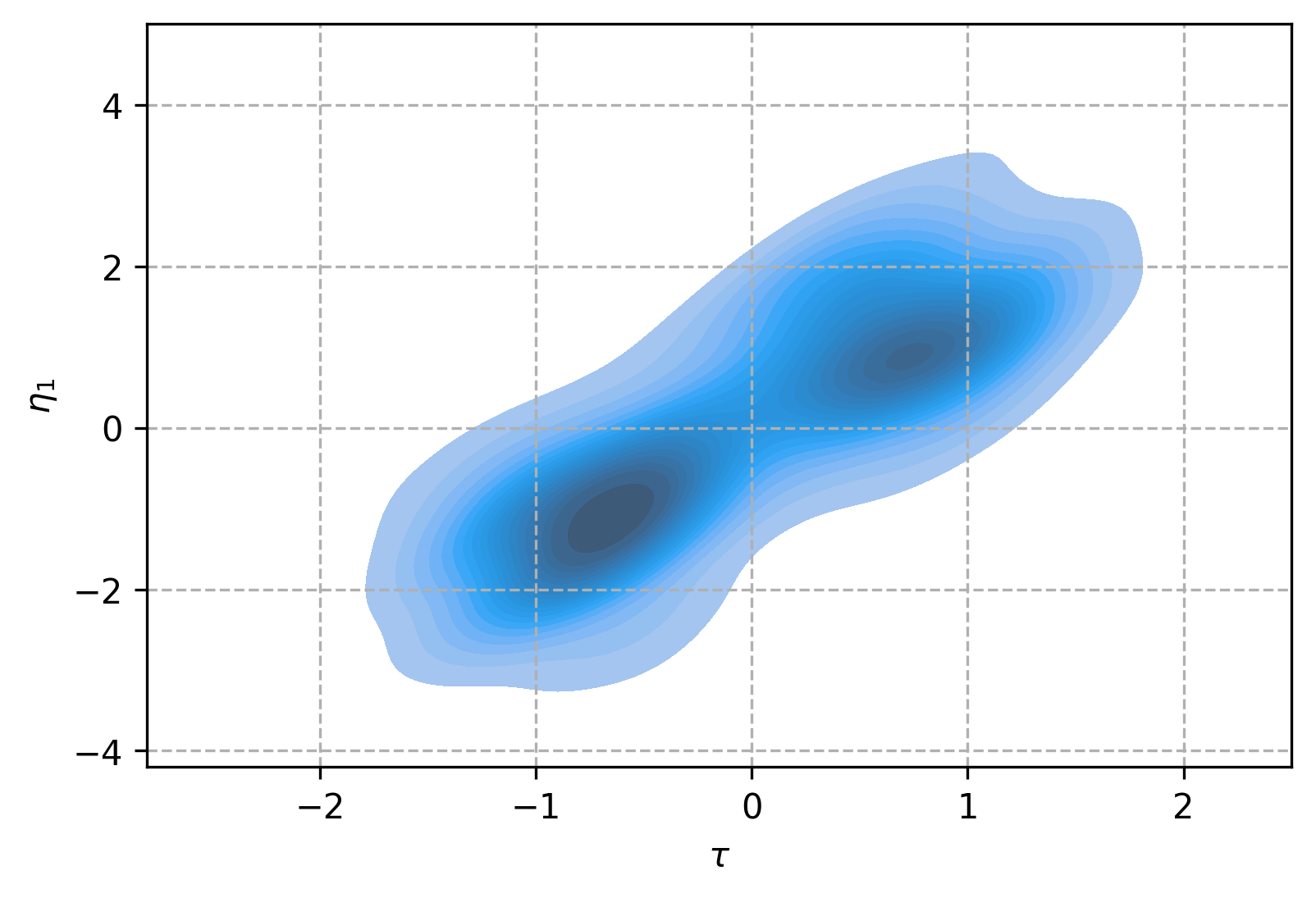
t-walk

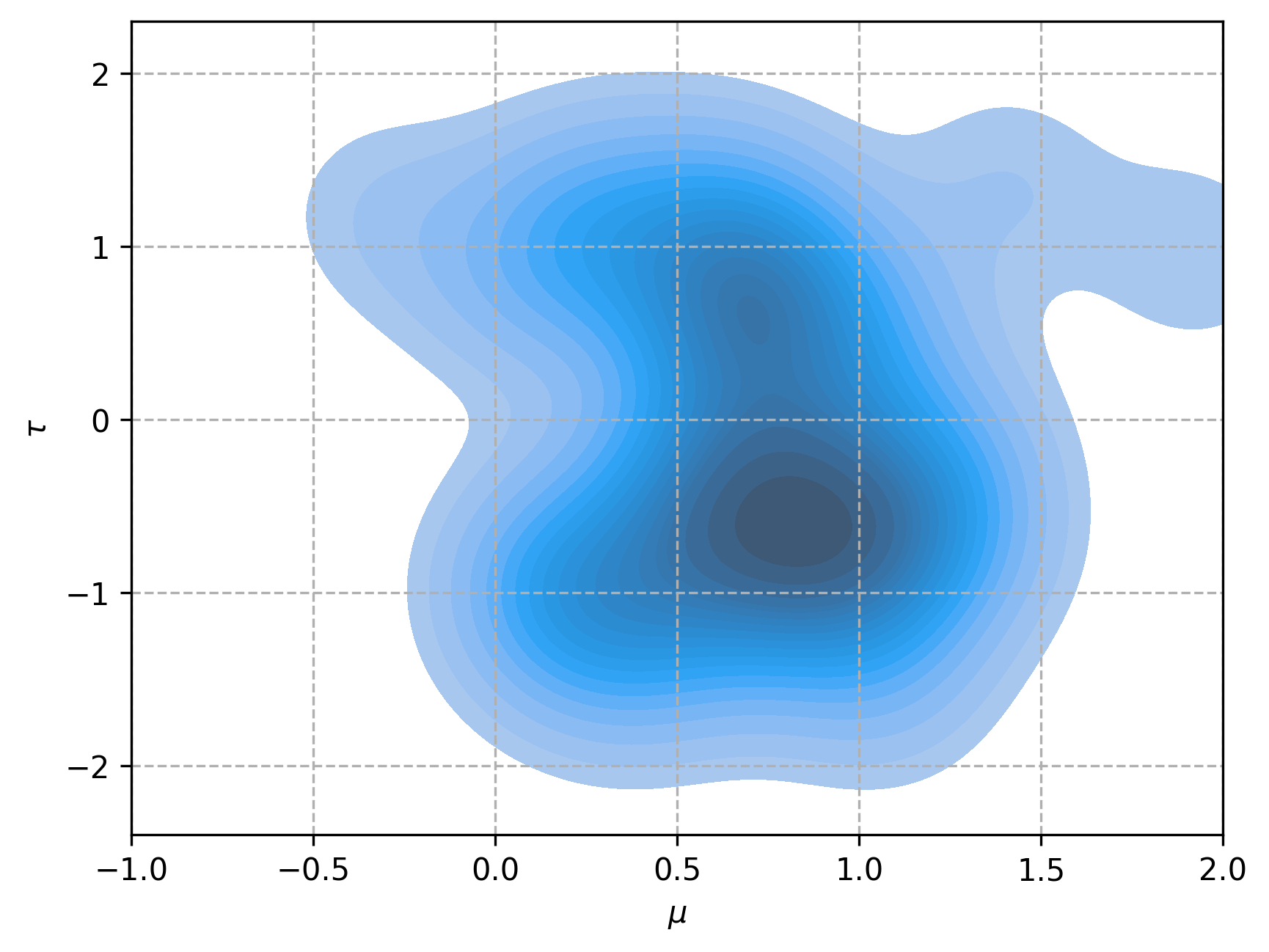
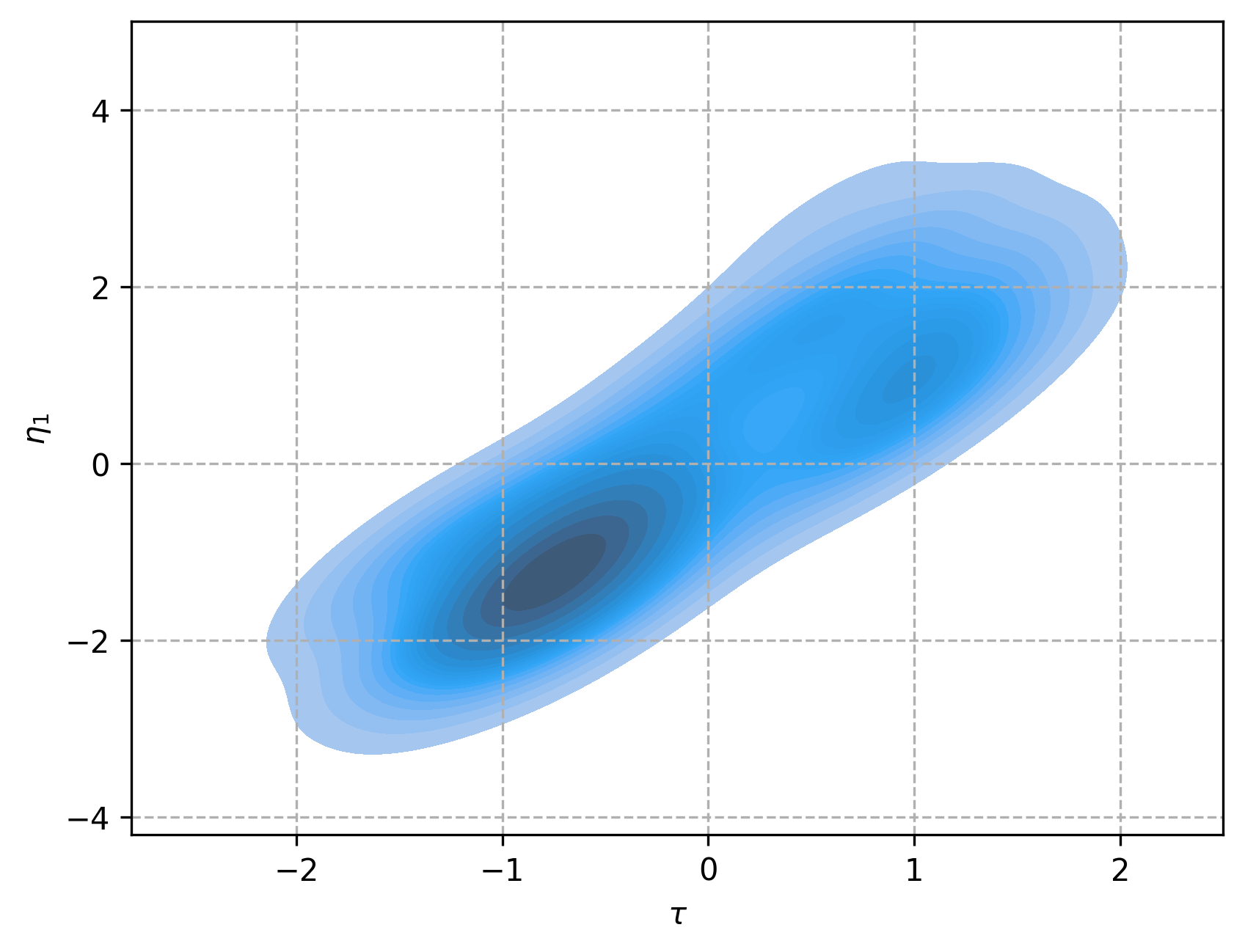
Figure 8: Densities of the marginal distributions $\left(\mu,\tau\right)$ and $\left(\tau,\eta_{1}\right)$ simulated from the Markov chain with target density $S^{\prime}$, for a chain of the size of 500,000 states with an effective sample of 14238, 218, and 46 generated with HMC, RWM, and t-walk, respectively.

Table 7: Comparison between HMC, RWMH, and t-walk, when simulating the target distribution with density $S^{\prime}$.

	HMC	RWMH	t-walk
Burn-in	100	200	200
lag	35	2300	11000
Acceptance rate	93.05%	24.68%	18.06%
Effective sample	14283	218	46
Execution time (s)	9968	4345	1070
Seconds per sample	0.698	19.93	23.36

As a final example, an effective sample of size 500 was generated with the HMC, RWMH, and t-walk methods, with the burn-in and lag periods determined for each method as outlined in the table 7. Figure 9 shows the densities of the marginal distributions $\left(\mu,\tau\right)$ and $\left(\tau,\eta_{1}\right)$ obtained in these simulations. Table 8 presents the differences between HMC, RWMH, and t-walk in terms of execution time, acceptance rates, and the number of iterations required. It is noteworthy that the time required for HMC to generate simulations is significantly less than that required for RWMH and t-walk.

HMC

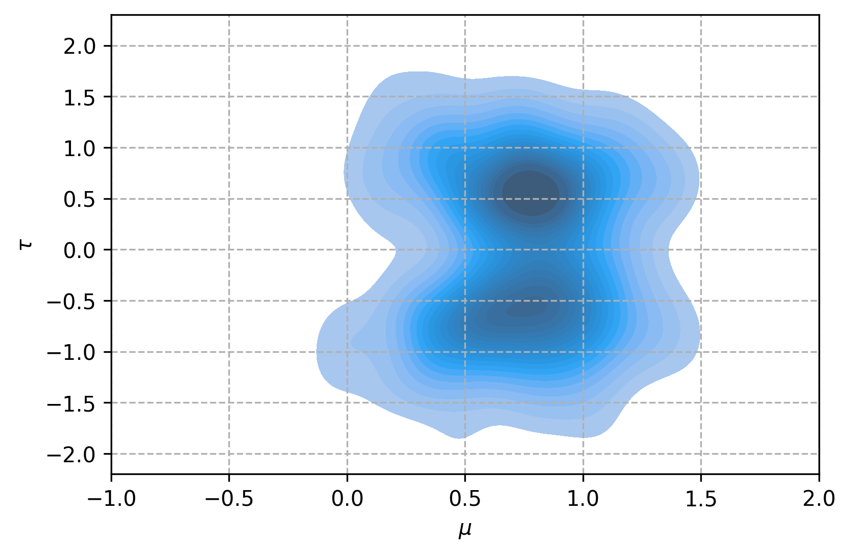
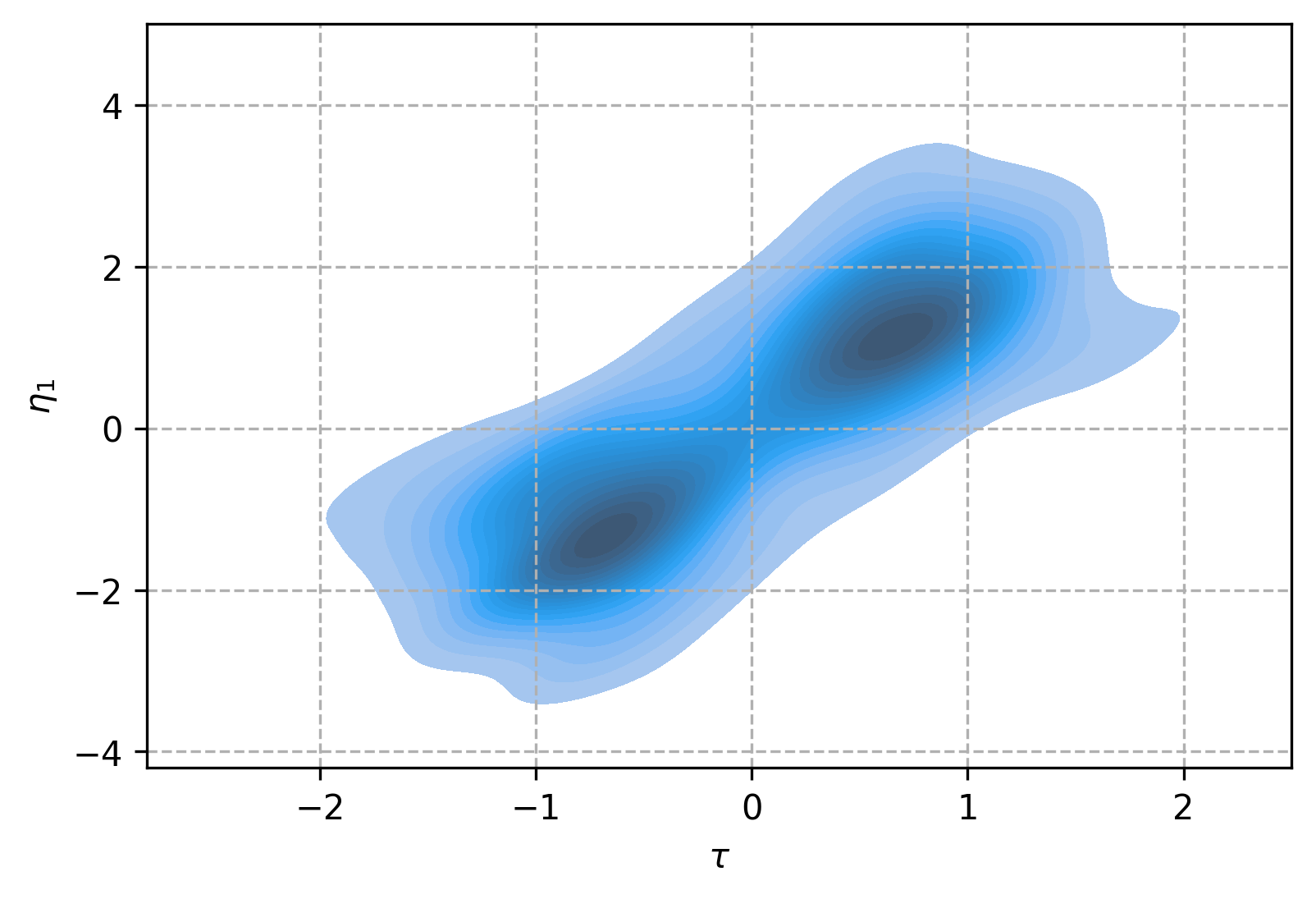
RWMH

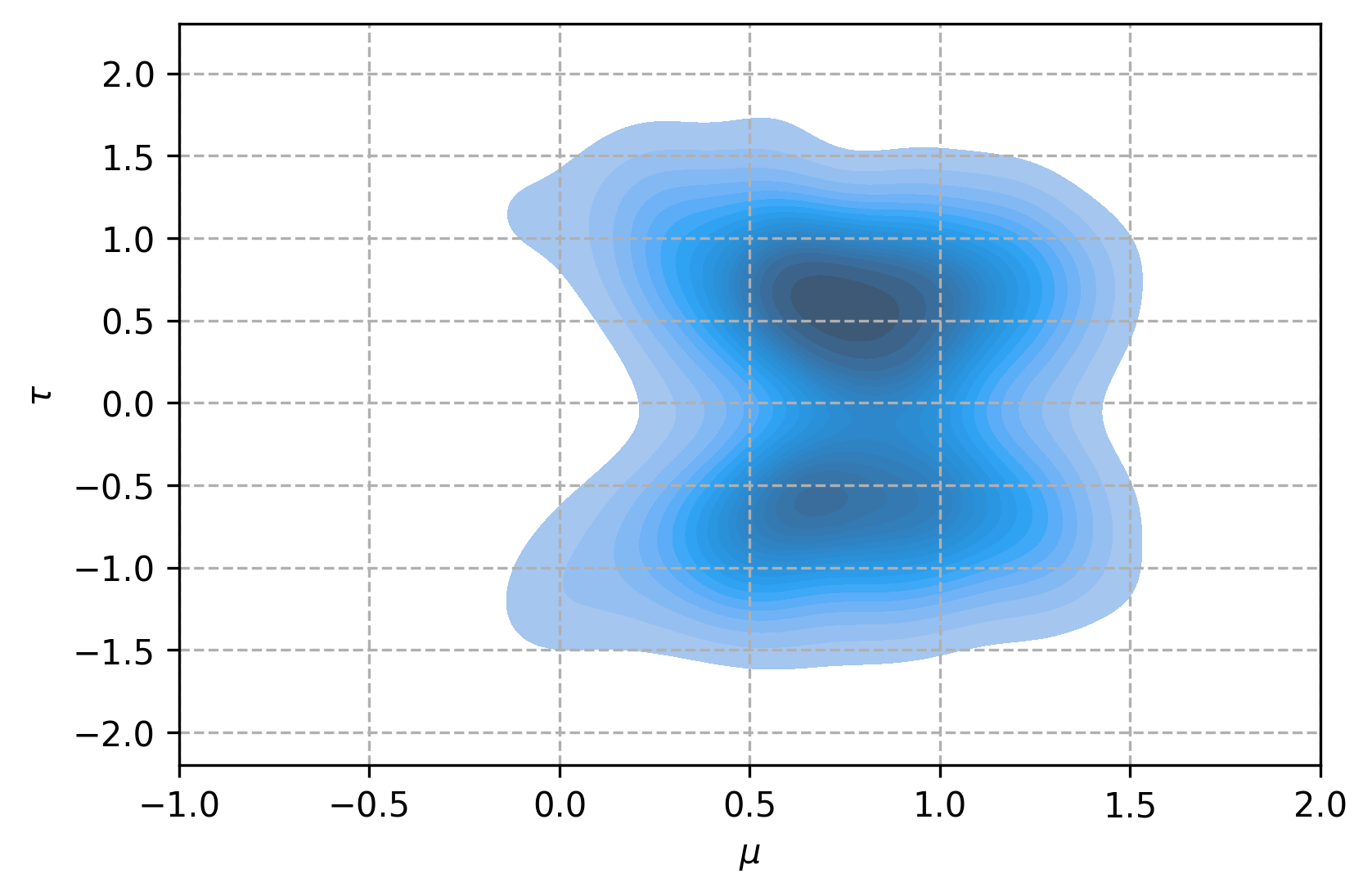
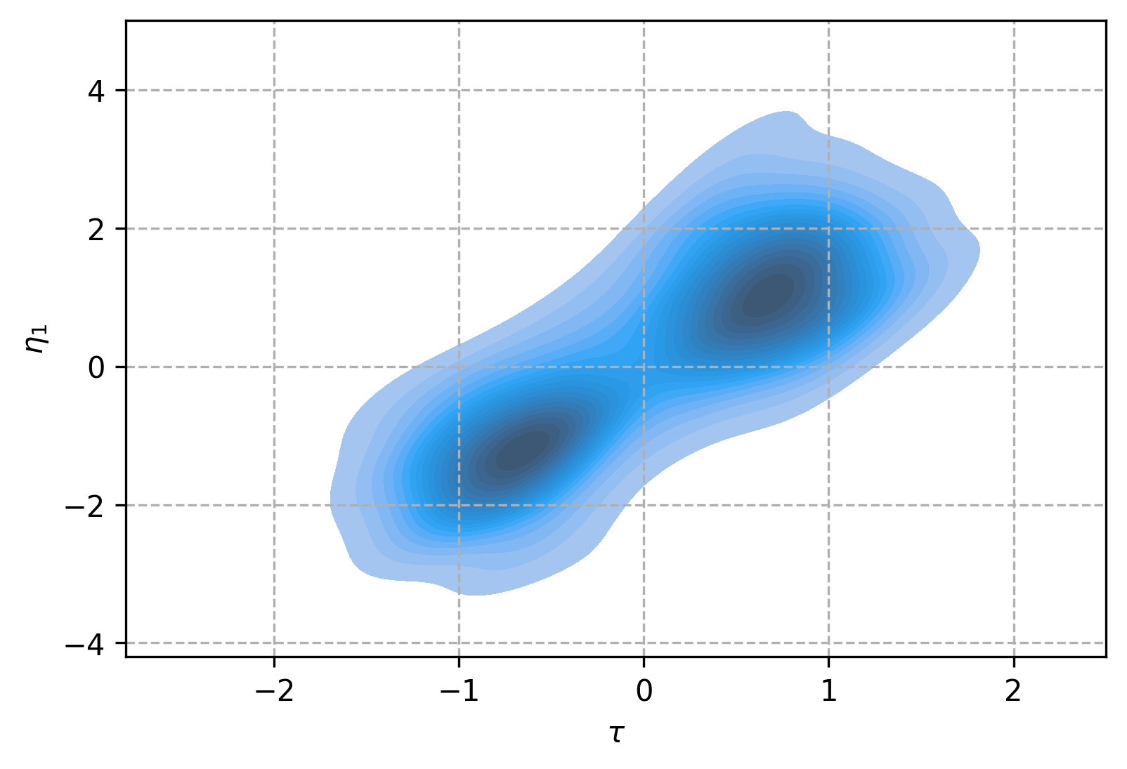
t-walk

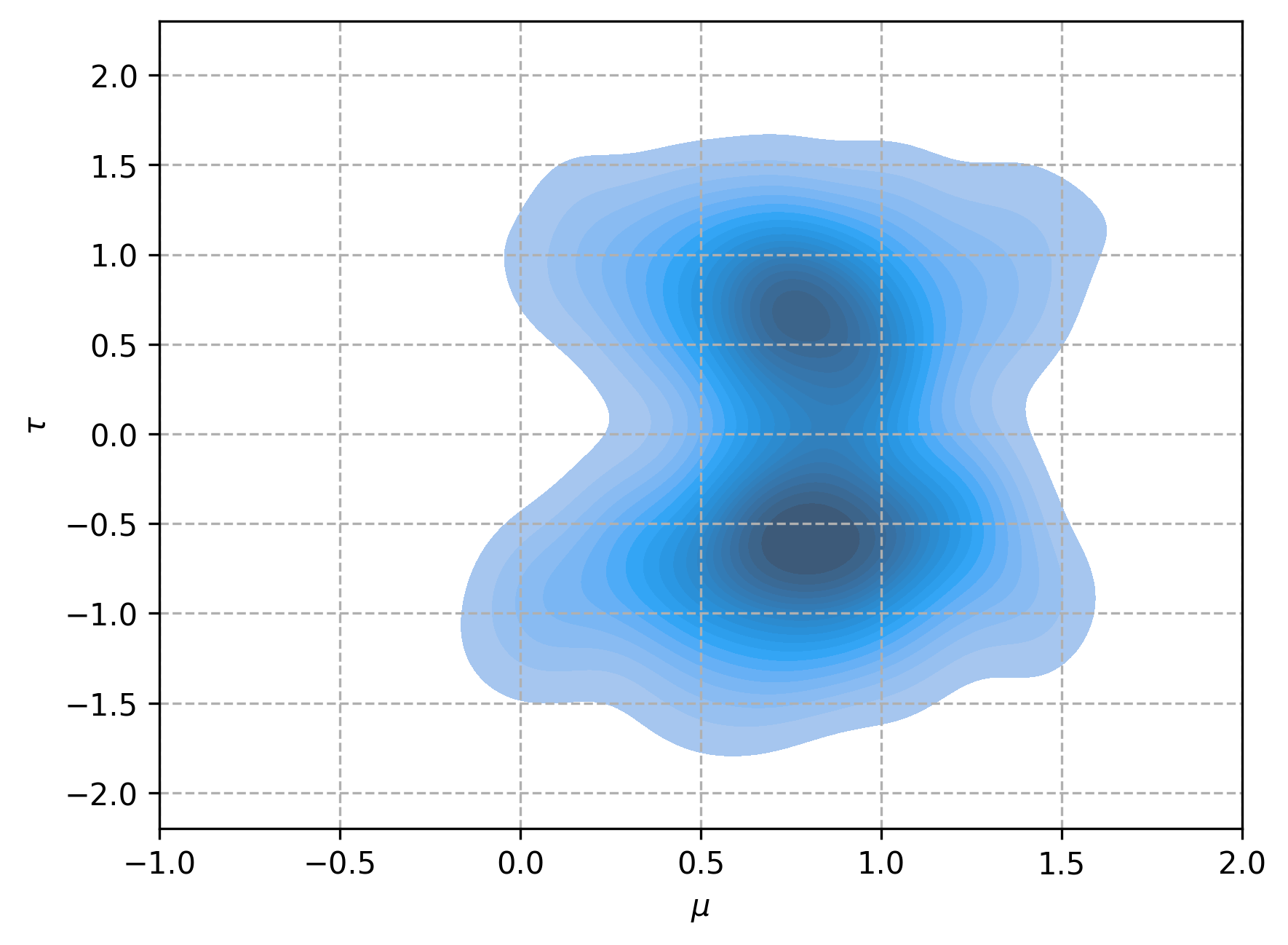
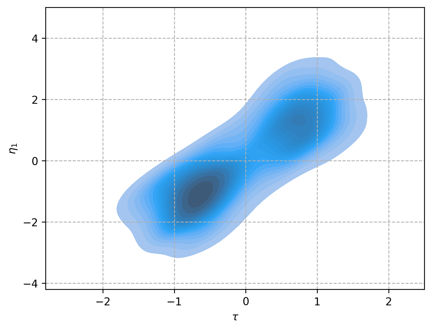
Figure 9: Density of the 500 samples simulated of the marginal distributions $\left(\mu,\tau\right)$ and $\left(\tau,\eta_{1}\right)$ with target density $S^{\prime}$.

Table 8: Comparison when simulating 500 samples of the target distribution with density $S^{\prime}$.

	HMC	RWMH	t-walk
Acceptance rate	92.49%	24.77%	18.25%
Execution time (s)	166	16861	11766
Simulations required	17,600	1,150,200	5,500,200

The Python code for this example can be found here.

5 Conclusions

In the comparative analysis of the HMC, RWMH and t-walk methods presented in Section 4, it can be observed that the HMC method exhibits superior efficiency in terms of time. The advantage of this method is due to the information it utilises regarding the gradient of the target density and the application of Hamiltonian dynamics, which renders the chain transitions suitable for exploring the target distribution.

Each iteration of the HMC method is more costly than those of the RWMH and t-walk algorithm due to the necessity of solving or approximating Hamilton’s equations. However, it is more efficient since HMC typically requires fewer iterations to obtain an effective sample of the target distribution, due to the shorter burn-in period. Furthermore, the autocorrelation of the states of the chain is typically significantly lower in HMC than in RWMH and t-walk.

A further crucial distinction between the HMC algorithm and RWMH is the optimal acceptance rates that they exhibit. As previously stated in section 3.1.1, the HMC has an optimal acceptance rate of 0.651 under specific assumptions. In the case of RWMH, an equivalent result is presented in [31], where it is mentioned that under certain assumptions, the optimal acceptance rate is 0.234. This is also a reason why the HMC algorithm is capable of retaining a greater number of simulations as an effective sample of the target distribution than RWMH.

It is important to note that HMC is not a definitive solution to the limitations of MCMC methods since, as shown in the example of section 4.3, it also encounters challenges when simulating distributions with multiple modes. In this instance, the t-walk algorithm demonstrated superior performance, as it was capable of simulating bimodal distributions.

Moreover, the time efficiency of the HMC method when making inferences of the model presented in Section 4.4 is noteworthy. As demonstrated in this example, it generates the simulations at a considerably faster rate than RWMH and t-walk.

It is crucial to underscore that the HMC method is constrained by a significant limitation: it necessitates knowledge of the gradient of the target density, which is frequently unavailable, thereby precluding its implementation.

Appendix A Classical Mechanics

Classical mechanics, also known as Newtonian mechanics, are generally considered to have been initiated in [28], where the foundations of classical mechanics are established by three laws of motion and the law of universal gravitation that unifies terrestrial and celestial mechanics. The object of study of Newtonian mechanics is to model the motion of particles, which are a mathematical abstraction representing bodies as points in space to which physical properties, such as mass, can be attributed in real and complete three-dimensional vector spaces.

According to [12] the motion of a particle can be described by a vectorial function $r\left(t\right)=\left(x(t),y(t),z(t)\right)$ which indicates the position of the particle at time $t$, as a function of each coordinate axis. The infinitesimal change of the position with respect to time is called velocity, is denoted by $v(t)$, and is calculated as the derivative of the position vector with respect to time, in mathematical notation

$$v(t)=\dfrac{dr\left(t\right)}{dt}=\left(\frac{dx(t)}{dt},\frac{dy(t)}{dt},\frac{dz(t)}{dt}\right).$$ (57)

The acceleration at time $t$ is defined as the infinitesimal change of velocity with respect to time. It is calculated as the derivative of the velocity vector and is denoted by $a\left(t\right)$, where

$$a(t)=\dfrac{dv\left(t\right)}{dt}=\left(\frac{d^{2}x(t)}{dt^{2}},\frac{d^{2}y(t)}{dt^{2}},\frac{d^{2}z(t)}{dt^{2}}\right).$$ (58)

A.1 Newton’s laws of motion

Newton’s laws of motion describe the movement of objects and how forces interact with them. In this section, we will introduce the three Newton’s laws consulted in [32].

The first law, also called the law of inertia, states that “A body continues to remain in a state of rest or moves with a uniform speed along a straight line unless subjected to an external force.”. This law, therefore, states that for a body to alter its motion, there must be some force that causes it to move, or in mathematical terms, where $F_{i}$ denotes the $i$-th force applied to a body,

$$\stackrel{{\scriptstyle[}}{{i}}=1]{n}{\sum}F_{i}\left(x(t),y(t),z(t)\right)=\left(0,0,0\right)\text{ \hskip 1.42271ptif \hskip 1.42271pt and \hskip 1.42271pt only \hskip 1.42271pt if \hskip 1.42271pt}\frac{dv}{dt}=\left(0,0,0\right),$$ (59)

that is, the resultant force applied to a particle is zero if and only if its velocity is not changed.

The second law mentions that in an inertial frame, i.e. a reference frame in which the first law is satisfied, “The rate of change of linear momentum of a body is proportional to the magnitude of the external force acting on it and takes place in the direction of that force.” Thus, Newton’s second law states that in an inertial frame, it is true that for any time $t$,

$$F\left(x(t),y(t),z(t)\right)=\dfrac{dv\left(t\right)}{dt}m\left(t\right),$$ (60)

where $m\left(t\right)$ and $F\left(t\right)$ represent the inertial mass and force at time $t$, respectively. From (60) follows the equation relating force to mass and acceleration

$$F\left(x(t),y(t),z(t)\right)=m\left(t\right)a\left(t\right).$$ (61)

Newton’s third law says that: “The forces exerted by two bodies on each other are equal in magnitude and opposite in direction.” This law is also known as the principle of action and reaction. It states that if one body applies a force on another, the latter will exert a force of equal magnitude and in the opposite direction on the former, i.e.,

$$f_{ij}=-f_{ji},$$ (62)

where $f_{ij}$ is the force produced by the action of body $i$ on body $j$.

A.2 Work and Kinetic Energy

In mechanics, a force applied to a particle is said to work when it can move it from one point to another. The definition of work is based on a line integral which is defined in [24].

The work, denoted by $W_{ab}$, in the case of a particle of mass $m$, moving according to a trajectory $C$ under the action of a resultant force $F$ dependent on the particle’s position, it is given by

$$W_{ab}=\int_{C}F\left(r\left(t\right)\right)\cdotp dr=\sideset{}{{}_{a}^{b}}{\int}F\left(r\left(t\right)\right)\cdotp\frac{dr\left(t\right)}{dt}dt,$$ (63)

where $r(t)$ is the parameterization of the curve $C$ along which the particle moves and $\frac{dr\left(t\right)}{dt}$ as defined in (57) is the velocity vector. Using Newton’s second law and assuming constant mass, $F=ma\left(t\right)$, it follows that

$$W_{ab} = \frac{m}{2}(v(b)^{2}-v(a)^{2}).$$ (64)

If a velocity-dependent function $T$ is defined, with the correspondence rule given by $T\left(v\left(t\right)\right)=\frac{1}{2}mv(t)^{2}$, we can rewrite (64) as

$$W_{ab}=T\left(v\left(b\right)\right)-T\left(v\left(a\right)\right).$$ (65)

$T\left(v\left(t\right)\right)$ is known as the particle’s kinetic energy at time $t$, so (65) states that the work done by a force is equal to the change in kinetic energy in time $b-a$. In mechanics, energy refers to the capacity of bodies to do work, and kinetic energy is that which a body possesses by the fact of being in motion.

A.3 Conservative Forces and Potential Energy

A conservative force field is one in which the work done by a force to move a particle from point A to point B is independent of the trajectory. By definition, in conservative force fields, for any trajectories $v$ and $w$ from point A to point B, it will be fulfilled that

$$\int_{w}F\left(r(t)\right)dr=\int_{v}F\left(r(t)\right)dr$$ (66)

or

$$\int_{w}F\left(r(t)\right)dr-\int_{v}F\left(r(t)\right)dr=0.$$ (67)

The left-hand side of the equality (67) can be rewritten as a line integral over a curve Z, defined as a closed path starting and ending at A and passing through point B, that is

$$\int_{Z}F\left(r(t)\right)dr=0.$$ (68)

To find the forces $F$ that satisfy the equality (68), Stokes’ theorem is used, which relates surface integrals to line integrals. Its proof can be found in [24]. Supported by Stokes’ theorem and equation (68), it follows that the conservative forces are those which, for some surface $S$,

$$\int_{S}(\nabla\times F)dS=0.$$ (69)

Let us note that $F=-\nabla U(r(t))$, where $U$ is a scalar function that depends on the position of the particle, satisfies the equation (69), because $\nabla\times(-\nabla U)=0$ as proved in [23]. Therefore, the conservative forces are those that can be written in the form

$$F=\left(-\frac{\partial U}{\partial x},-\frac{\partial U}{\partial y},-\frac{\partial U}{\partial z}\right)=-\nabla U\left(r\left(t\right)\right).$$ (70)

The value $U\left(r\left(t\right)\right)$ in (70) is known as the potential energy and refers to the energy a particle possesses due to its position.

The mechanical energy of a system of particles at a time $t$, denoted by $E\left(t\right)$, is defined as the sum of the kinetic energy and the potential energy of the system, which is formulated as

$$E\left(t\right)=T\left(v\left(t\right)\right)+U\left(r\left(t\right)\right).$$ (71)

The mechanical energy is conserved, i.e., does not change over time since $~\frac{dE\left(t\right)}{dt}=0$ as shown in [27]. This result is known as the law of conservation of energy.

References

- [1] {barticle}[author] \bauthor\bsnmAndrieu, \bfnmC\binitsC., \bauthor\bsnmDoucet, \bfnmA\binitsA. and \bauthor\bsnmRobert, \bfnmCP\binitsC. (\byear2004). \btitleComputational advances for and from Bayesian analysis. \bjournalStatistical science \bpages118–127. \endbibitem
- [2] {barticle}[author] \bauthor\bsnmApte, \bfnmMohit\binitsM. (\byear2024). \btitleRefining Credit Risk Analysis-Integrating Bayesian MCMC with Hamiltonian Monte Carlo. \bjournalInternational Journal of Innovative Research in Computer Science & Technology \bvolume12 \bpages88–91. \endbibitem
- [3] {barticle}[author] \bauthor\bsnmBeskos, \bfnmAlexandros\binitsA., \bauthor\bsnmPillai, \bfnmNatesh\binitsN., \bauthor\bsnmRoberts, \bfnmGareth\binitsG., \bauthor\bsnmSanz-Serna, \bfnmJesus-Maria\binitsJ.-M., \bauthor\bsnmStuart, \bfnmAndrew\binitsA. \betalet al. (\byear2013). \btitleOptimal tuning of the hybrid Monte Carlo algorithm. \bjournalBernoulli \bvolume19 \bpages1501–1534. \endbibitem
- [4] {bbook}[author] \bauthor\bsnmBorzì, \bfnmAlfio\binitsA. (\byear2020). \btitleModelling with Ordinary Differential Equations: A Comprehensive Approach. \bpublisherCRC Press. \endbibitem
- [5] {bbook}[author] \bauthor\bsnmBrooks, \bfnmSteve\binitsS., \bauthor\bsnmGelman, \bfnmAndrew\binitsA., \bauthor\bsnmJones, \bfnmGalin\binitsG. and \bauthor\bsnmMeng, \bfnmXiao-Li\binitsX.-L. (\byear2011). \btitleHandbook of markov chain monte carlo. \bpublisherCRC press. \endbibitem
- [6] {barticle}[author] \bauthor\bsnmChristen, \bfnmJ Andrés\binitsJ. A. and \bauthor\bsnmFox, \bfnmColin\binitsC. (\byear2010). \btitleA general purpose sampling algorithm for continuous distributions (the t-walk). \bjournalBayesian Analysis \bvolume5 \bpages263–281. \endbibitem
- [7] {barticle}[author] \bauthor\bsnmCordeiro, \bfnmCEZ\binitsC., \bauthor\bsnmStutz, \bfnmLT\binitsL., \bauthor\bsnmKnupp, \bfnmDC\binitsD. and \bauthor\bsnmMatt, \bfnmCFT\binitsC. (\byear2022). \btitleGeneralized integral transform and Hamiltonian Monte Carlo for Bayesian structural damage identification. \bjournalApplied Mathematical Modelling \bvolume104 \bpages243–258. \endbibitem
- [8] {bbook}[author] \bauthor\bparticledel \bsnmCastillo, \bfnmGerardo F Torres\binitsG. F. T. (\byear2018). \btitleAn Introduction to Hamiltonian Mechanics. \bpublisherSpringer. \endbibitem
- [9] {barticle}[author] \bauthor\bsnmDelina, \bfnmMutia\binitsM., \bauthor\bsnmMajid, \bfnmIrsyad Tio\binitsI. T. and \bauthor\bsnmFauzan, \bfnmAhmad\binitsA. (\byear2022). \btitleThe Simulation of Covid-19 Droplet Transmission with Hamiltonian Monte Carlo Method. \bjournalIndo. J. Appl. Phys \bvolume12 \bpages12. \endbibitem
- [10] {barticle}[author] \bauthor\bsnmDurmus, \bfnmAlain\binitsA., \bauthor\bsnmMoulines, \bfnmÉric\binitsÉ. and \bauthor\bsnmSaksman, \bfnmEero\binitsE. (\byear2020). \btitleIrreducibility and geometric ergodicity of Hamiltonian Monte Carlo. \bjournalThe Annals of Statistics \bvolume48 \bpages3545–3564. \endbibitem
- [11] {barticle}[author] \bauthor\bsnmFreedman, \bfnmGabriel E\binitsG. E., \bauthor\bsnmJohnson, \bfnmAaron D\binitsA. D., \bauthor\bparticlevan \bsnmHaasteren, \bfnmRutger\binitsR. and \bauthor\bsnmVigeland, \bfnmSarah J\binitsS. J. (\byear2023). \btitleEfficient gravitational wave searches with pulsar timing arrays using Hamiltonian Monte Carlo. \bjournalPhysical Review D \bvolume107 \bpages043013. \endbibitem
- [12] {barticle}[author] \bauthor\bsnmGallavotti, \bfnmG.\binitsG. (\byear2006). \btitleIntroductory Article: Classical Mechanics. \bpages1-33. \endbibitem
- [13] {bbook}[author] \bauthor\bsnmGarrigós, \bfnmJosep Español\binitsJ. E., \bauthor\bsnmMaestro, \bfnmMaría del Mar Serrano\binitsM. d. M. S. and \bauthor\bsnmLópez, \bfnmIgnacio Zúñiga\binitsI. Z. (\byear2012). \btitleMecánica clásica. \bpublisherEditorial UNED. \endbibitem
- [14] {bbook}[author] \bauthor\bsnmGelman, \bfnmAndrew\binitsA., \bauthor\bsnmCarlin, \bfnmJohn B\binitsJ. B., \bauthor\bsnmStern, \bfnmHal S\binitsH. S., \bauthor\bsnmDunson, \bfnmDavid B\binitsD. B., \bauthor\bsnmVehtari, \bfnmAki\binitsA. and \bauthor\bsnmRubin, \bfnmDonald B\binitsD. B. (\byear2013). \btitleBayesian data analysis. \bpublisherCRC press. \endbibitem
- [15] {bmisc}[author] \bauthor\bsnmGilks, \bfnmRichardson\binitsR. and \bauthor\bsnmRichardson, \bfnmS\binitsS. (\byear1996). \btitleSpiegelhalter. Markov Chain Monte Carlo in practice. \endbibitem
- [16] {bbook}[author] \bauthor\bsnmGreiner, \bfnmWalter\binitsW. (\byear2009). \btitleClassical mechanics: systems of particles and Hamiltonian dynamics. \bpublisherSpringer Science & Business Media. \endbibitem
- [17] {bbook}[author] \bauthor\bsnmHairer, \bfnmErnst\binitsE., \bauthor\bsnmLubich, \bfnmChristian\binitsC. and \bauthor\bsnmWanner, \bfnmGerhard\binitsG. (\byear2006). \btitleGeometric numerical integration: structure-preserving algorithms for ordinary differential equations \bvolume31. \bpublisherSpringer Science & Business Media. \endbibitem
- [18] {barticle}[author] \bauthor\bsnmHaq, \bfnmMuhammad Tahmidul\binitsM. T., \bauthor\bsnmZlatkovic, \bfnmMilan\binitsM. and \bauthor\bsnmKsaibati, \bfnmKhaled\binitsK. (\byear2022). \btitleOccupant injury severity in passenger car-truck collisions on interstate 80 in Wyoming: a Hamiltonian Monte Carlo Markov Chain Bayesian inference approach. \bjournalJournal of Transportation Safety & Security \bvolume14 \bpages498–522. \endbibitem
- [19] {barticle}[author] \bauthor\bsnmHastings, \bfnmW Keith\binitsW. K. (\byear1970). \btitleMonte Carlo sampling methods using Markov chains and their applications. \endbibitem
- [20] {barticle}[author] \bauthor\bsnmJarner, \bfnmSøren Fiig\binitsS. F. and \bauthor\bsnmHansen, \bfnmErnst\binitsE. (\byear2000). \btitleGeometric ergodicity of Metropolis algorithms. \bjournalStochastic processes and their applications \bvolume85 \bpages341–361. \endbibitem
- [21] {bbook}[author] \bauthor\bsnmLiang, \bfnmFaming\binitsF., \bauthor\bsnmLiu, \bfnmChuanhai\binitsC. and \bauthor\bsnmCarroll, \bfnmRaymond\binitsR. (\byear2011). \btitleAdvanced Markov chain Monte Carlo methods: learning from past samples \bvolume714. \bpublisherJohn Wiley & Sons. \endbibitem
- [22] {barticle}[author] \bauthor\bsnmLivingstone, \bfnmSamuel\binitsS., \bauthor\bsnmBetancourt, \bfnmMichael\binitsM., \bauthor\bsnmByrne, \bfnmSimon\binitsS., \bauthor\bsnmGirolami, \bfnmMark\binitsM. \betalet al. (\byear2019). \btitleOn the geometric ergodicity of Hamiltonian Monte Carlo. \bjournalBernoulli \bvolume25 \bpages3109–3138. \endbibitem
- [23] {bbook}[author] \bauthor\bsnmMann, \bfnmPeter\binitsP. (\byear2018). \btitleLagrangian and Hamiltonian dynamics. \bpublisherOxford University Press. \endbibitem
- [24] {bbook}[author] \bauthor\bsnmMarsden, \bfnmJerrold E\binitsJ. E., \bauthor\bsnmTromba, \bfnmAnthony J\binitsA. J. and \bauthor\bsnmMuñiz, \bfnmPatricio Cifuentes\binitsP. C. (\byear1991). \btitleCálculo vectorial \bvolume69. \bpublisherAddison-Wesley Iberoamericana. \endbibitem
- [25] {barticle}[author] \bauthor\bsnmMedina-Aguayo, \bfnmFelipe J\binitsF. J. and \bauthor\bsnmChristen, \bfnmJ Andrés\binitsJ. A. (\byear2020). \btitlePenalised t-walk MCMC. \bjournalarXiv preprint arXiv:2012.02293. \endbibitem
- [26] {binproceedings}[author] \bauthor\bsnmMescheder, \bfnmLars\binitsL., \bauthor\bsnmNowozin, \bfnmSebastian\binitsS. and \bauthor\bsnmGeiger, \bfnmAndreas\binitsA. (\byear2017). \btitleAdversarial variational bayes: Unifying variational autoencoders and generative adversarial networks. In \bbooktitleInternational Conference on Machine Learning \bpages2391–2400. \bpublisherPMLR. \endbibitem
- [27] {bbook}[author] \bauthor\bsnmMorin, \bfnmDavid\binitsD. (\byear2008). \btitleIntroduction to classical mechanics: with problems and solutions. \bpublisherCambridge University Press. \endbibitem
- [28] {bbook}[author] \bauthor\bsnmNewton, \bfnmIsaac\binitsI. (\byear1833). \btitlePhilosophiae naturalis principia mathematica \bvolume1. \bpublisherG. Brookman. \endbibitem
- [29] {barticle}[author] \bauthor\bsnmPetersen, \bfnmKaare Brandt\binitsK. B. and \bauthor\bsnmPedersen, \bfnmMichael Syskind\binitsM. S. (\byear2012). \btitleThe matrix cookbook, nov 2012. \bjournalURL http://www2. imm. dtu. dk/pubdb/p. php \bvolume3274 \bpages14. \endbibitem
- [30] {barticle}[author] \bauthor\bsnmPonce, \bfnmVictor Hugo\binitsV. H. (\byear2010). \btitleMecánica clásica. \bjournalMendoza: EDIUNC. \endbibitem
- [31] {barticle}[author] \bauthor\bsnmRoberts, \bfnmGareth O\binitsG. O., \bauthor\bsnmRosenthal, \bfnmJeffrey S\binitsJ. S. \betalet al. (\byear2001). \btitleOptimal scaling for various Metropolis-Hastings algorithms. \bjournalStatistical science \bvolume16 \bpages351–367. \endbibitem
- [32] {bbook}[author] \bauthor\bsnmRoy, \bfnmNikhil Ranjan\binitsN. R. (\byear1990). \btitleIntroduction to classical mechanics. \bpublisherVikas Publishing House. \endbibitem
- [33] {barticle}[author] \bauthor\bsnmSusik, \bfnmMateusz\binitsM., \bauthor\bsnmSchönborn, \bfnmHolger\binitsH. and \bauthor\bsnmSbalzarini, \bfnmIvo F\binitsI. F. (\byear2022). \btitleHamiltonian Monte Carlo with strict convergence criteria reduces run-to-run variability in forensic DNA mixture deconvolution. \bjournalForensic Science International: Genetics \bvolume60 \bpages102744. \endbibitem
- [34] {barticle}[author] \bauthor\bsnmSusik, \bfnmMateusz\binitsM., \bauthor\bsnmSchönborn, \bfnmHolger\binitsH. and \bauthor\bsnmSbalzarini, \bfnmIvo F\binitsI. F. (\byear2022). \btitleHamiltonian Monte Carlo with strict convergence criteria reduces run-to-run variability in forensic DNA mixture deconvolution. \bjournalForensic Science International: Genetics \bvolume60 \bpages102744. \endbibitem
- [35] {barticle}[author] \bauthor\bsnmTierney, \bfnmLuke\binitsL. (\byear1994). \btitleMarkov chains for exploring posterior distributions. \bjournalthe Annals of Statistics \bpages1701–1728. \endbibitem
- [36] {barticle}[author] \bauthor\bsnmZhao, \bfnmYidong\binitsY., \bauthor\bsnmTourais, \bfnmJoao\binitsJ., \bauthor\bsnmPierce, \bfnmIain\binitsI., \bauthor\bsnmNitsche, \bfnmChristian\binitsC., \bauthor\bsnmTreibel, \bfnmThomas A\binitsT. A., \bauthor\bsnmWeingärtner, \bfnmSebastian\binitsS., \bauthor\bsnmSchweidtmann, \bfnmArtur M\binitsA. M. and \bauthor\bsnmTao, \bfnmQian\binitsQ. (\byear2024). \btitleBayesian Uncertainty Estimation by Hamiltonian Monte Carlo: Applications to Cardiac MRI Segmentation. \bjournalarXiv preprint arXiv:2403.02311. \endbibitem