Recurrence Plots for the Analysis of Complex Systems

, , ,

List of Abbreviations and Symbols

$\langle x\rangle$	mean of series $x$, expectation value of $x$
$\bar{x}$	series $x$ normalised to zero mean and standard deviation of one
$\hat{x}$	estimator for $x$
$\delta(\cdot)$	delta function ($\delta(x)=\{1\,|\,x=0;\ 0\,|\,x\not=0\}$)
$\delta(\cdot,\cdot)$	Kronecker delta function ($\delta(x,y)=\{1\,|\,x=y;\ 0\,|\,x\not=y\}$)
$\partial_{t}(\cdot)$	derivative with respect to time ($\partial_{t}(x)=\frac{d}{dt}$)
$\Delta t$	sampling time
$\varepsilon$	radius of neighbourhood (threshold for RP computation)
$\lambda$	Lyapunov exponent
$\mu(\cdot)$	probability measure
$\Omega$	frequency
$\pi$	order pattern
$\Phi$	phase
$\sigma$	standard deviation
$\Theta(\cdot)$	Heaviside function ($\Theta(x)=\{1\,|\,x>0;\ 0\,|\,x\leq 0\}$)
$\tau$	time delay (index-based units)
$\xi$	white noise
$\mathcal{A}$	a measurable set
$B_{\vec{x}_{i}}(\varepsilon)$	the $\varepsilon$-neighbourhood around the point $\vec{x}_{i}$ on the trajectory
$\mathrm{cov}(\cdot)$	(auto)covariance function
$C_{d}(\varepsilon)$	correlation sum for a system of dimension $d$ and by using a threshold $\varepsilon$
$CC(\varepsilon)$	cross correlation sum for two systems using a threshold $\varepsilon$
$\mathbf{CR}(\varepsilon)$	cross recurrence matrix between two phase space trajectories
	by using a neighbourhood size $\varepsilon$
$CPR$	synchronisation index based on recurrence probabilities
CRP	cross recurrence plot
CS	complete synchronisation
$\mathbf{D}$	distance matrix between phase space vectors
$D$	distance
$D_{1}$	information dimension
$D_{2}$	correlation dimension
$D_{P}$	point-wise dimension
$DET$	measure for recurrence quantification: determinism
$DET_{\tau}$	measure for recurrence quantification: determinism of the $\tau^{\text{th}}$
	diagonal in the RP
$DIV$	measure for recurrence quantification: divergence
$d$	dimension of the system
$ENTR$	measure for recurrence quantification: entropy
FAN	fixed amount of nearest neighbours (neighbourhood criterion)
FNN	false nearest neighbour
GS	generalised synchronisation
$H_{q}$	Renyi entropy of order $q$
$h_{D}$	topological dimension
$I_{q}$	generalised mutual information (redundancy) of order $q$
$i,j,k$	indices
$JC(\varepsilon_{1},\varepsilon_{2})$	joint correlation sum for two systems using thresholds $\varepsilon_{1}$ and $\varepsilon_{2}$
$JK_{2}$	joint Renyi entropy of 2${}^{\text{nd}}$ order
$JPR$	joint probability of recurrence
JRP	joint recurrence plot
$K_{2}$	Renyi entropy of 2${}^{\text{nd}}$ order (correlation entropy)
$L$	measure for recurrence quantification: average line length of
	diagonal lines
$L_{\tau}$	measure for recurrence quantification: average line length of
	diagonal lines of the $\tau^{\text{th}}$ diagonal in the RP
$L_{\text{max}}$	measure for recurrence quantification: length of the longest
	diagonal line
$L_{p}$-norm	vector norm, e.g. the Euclidean norm ($L_{2}$-norm), Maximum
	norm ($L_{\infty}$-norm)
$l_{\text{min}}$	predefined minimal length of a diagonal line
$LAM$	measure for recurrence quantification: laminarity
LOI	line of identity (the main diagonal line in a RP, $\mathbf{R}_{i,\,i}=1$)
LOS	line of synchronisation (the distorted main diagonal line in a CRP)
$MFNN$	Mutual false nearest neighbours
$m$	embedding dimension
$N$	length of a data series
$N_{\text{l}}$, $N_{\text{v}}$	number of diagonal/vertical lines
$N_{\text{n}}$	number of (nearest) neighbours
$\mathds{N}$	set of natural numbers
OPRP	order patterns recurrence plot
$\mathbf{P}_{i,j}$	probability to find a recurrence point at $(i,j)$
$P(\cdot)$	histogram
$P(\varepsilon,l)$	histogram or frequency distribution of line lengths
$p(\cdot)$	probability
$p(\varepsilon,\tau)$	probability that the trajectory recurs after $\tau$ time steps
$p(\varepsilon,l)$	probability to find a line of exactly length $l$
$p_{c}(\varepsilon,l)$	probability to find a line of at least length $l$
PS	phase synchronisation
$Q(\tau)$	CRP symmetry measure
$q(\tau)$	CRP asymmetry measure
$q$	order
$\mathds{R}$	set of real numbers
$\mathcal{R}$	set of recurrence points
$\mathbf{R}(\varepsilon)$	recurrence matrix of a phase space trajectory by using
	a neighbourhood size $\varepsilon$
$R$	mean resultant length of phase vectors (synchronisation measure)
RATIO	measure for recurrence quantification: ratio between $DET$ and $RR$
RP	recurrence plot
RQA	recurrence quantification analysis
$RR$, $REC$	measure for recurrence quantification: recurrence rate (percent
	recurrence)
$RR_{\tau}$	measure for recurrence quantification: recurrence rate of the $\tau^{\text{th}}$
	diagonal in the RP
$S$	synchronisation index based on joint recurrence
$T^{(1)}$	recurrence time of $1^{st}$ type
$T^{(2)}$	recurrence time of $2^{nd}$ type
$T_{\text{ph}}$	phase period
$T_{\text{rec}}$	recurrence period
$TREND$	measure for recurrence quantification: trend
$TT$	measure for recurrence quantification: trapping time
$V_{\text{max}}$	measure for recurrence quantification: length of the longest vertical line
$v_{\text{min}}$	predefined minimal length of a vertical line
$\mathcal{X}$	a measurable set

1 Introduction

El poeta tiene dos obligaciones sagradas: partir y regresar.
(The poet has two holy duties: to set out and to return.)

Pablo Neruda

If we observe the sky on a hot and humid day in summer, we often “feel” that a thunderstorm is brewing. When children play, mothers often know instinctively when a situation is going to turn out dangerous. Each time we throw a stone, we can approximately predict where it is going to hit the ground. Elephants are able to find food and water during times of drought. These predictions are not based on the evaluation of long and complicated sets of mathematical equations, but rather on two facts which are crucial for our daily life:

1. similar situations often evolve in a similar way;

2. some situations occur over and over again.

The first fact is linked to a certain determinism in many real world systems. Systems of very different kinds, from very large to very small time-space scales can be modelled by (deterministic) differential equations. On very large scales we might think of the motions of planets or even galaxies, on intermediate scales of a falling stone and on small scales of the firing of neurons. All of these systems can be described by the same mathematical tool of differential equations. They behave deterministically in the sense that in principle we can predict the state of such a system to any precision and forever once the initial conditions are exactly known. Chaos theory has taught us that some systems – even though deterministic – are very sensitive to fluctuations and even the smallest perturbations of the initial conditions can make a precise prediction on long time scales impossible. Nevertheless, even for these chaotic systems short-term prediction is practicable.

The second fact is fundamental to many systems and is probably one of the reasons why life has developed memory. Experience allows remembering similar situations, making predictions and, hence, helps to survive. But remembering similar situations, e. g., the hot and humid air in summer which might eventually lead to a thunderstorm, is only helpful if a system (such as the atmospheric system) returns or recurs to former states. Such a recurrence is a fundamental characteristic of many dynamical systems.

They can indeed be used to study the properties of many systems, from astrophysics (where recurrences have actually been introduced) over engineering, electronics, financial markets, population dynamics, epidemics and medicine to brain dynamics. The methods described in this review are therefore of interest to scientists working in very different areas of research.

The formal concept of recurrences was introduced by Henri Poincaré in his seminal work from 1890 [1], for which he won a prize sponsored by King Oscar II of Sweden and Norway on the occasion of his majesty’s 60${}^{\text{th}}$ birthday. Therein, Poincaré did not only discover the “homoclinic tangle” which lies at the root of the chaotic behaviour of orbits, but he also introduced (as a by-product) the concept of recurrences in conservative systems. When speaking about the restricted three body problem he mentioned: “In this case, neglecting some exceptional trajectories, the occurrence of which is infinitely improbable, it can be shown, that the system recurs infinitely many times as close as one wishes to its initial state.” (translated from [1]) Even though much mathematical work was carried out in the following years, Poincaré’s pioneering work and his discovery of recurrence had to wait for more than 70 years for the development of fast and efficient computers to be exploited numerically. The use of powerful computers boosted chaos theory and allowed to study new and exciting systems. Some of the tedious computations needed to use the concept of recurrence for more practical purposes could only be made with this digital tool.

In 1987, Eckmann et al. introduced the method of recurrence plots (RPs) to visualise the recurrences of dynamical systems. Suppose we have a trajectory $\{\vec{x}_{i}\}_{i=1}^{N}$ of a system in its phase space [2]. The components of these vectors could be, e. g., the position and velocity of a pendulum or quantities such as temperature, air pressure, humidity and many others for the atmosphere. The development of the systems is then described by a series of these vectors, representing a trajectory in an abstract mathematical space. Then, the corresponding RP is based on the following recurrence matrix

$$\mathbf{R}_{i,j}=\begin{cases}1:\vec{x}_{i}\approx\vec{x}_{j}\\ 0:\vec{x}_{i}\not\approx\vec{x}_{j}\end{cases}\quad i,j=1,\ldots,N.$$ (1)

where $N$ is the number of considered states and $\vec{x}_{i}\approx\vec{x}_{j}$ means equality up to an error (or distance) $\varepsilon$. Note that this $\varepsilon$ is essential as systems often do not recur exactly to a formerly visited state but just approximately. Roughly speaking, the matrix compares the states of a system at times $i$ and $j$. If the states are similar, this is indicated by a one in the matrix, i. e. $\mathbf{R}_{i,j}=1$. If on the other hand the states are rather different, the corresponding entry in the matrix is $\mathbf{R}_{i,j}=0$. So the matrix tells us when similar states of the underlying system occur. This report shows that much more can be concluded from the recurrence matrix, Eq. (1). But before going into details, we use Eckmann’s representation of the recurrence matrix, to give the reader a first impression of the patterns of recurrences which will allow studying dynamical systems and their trajectories.

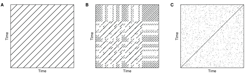
Figure 1: Recurrence plots of (A) a periodic motion with one frequency, (B) the chaotic Rössler system (Eq. (• ‣ A) with parameters $a=b=0.2$ and $c=5.7$) and (C) of uniformly distributed noise.

Let us consider the RPs of three prototypical systems, namely of a periodic motion on a circle (Fig. 1A), of the chaotic Rössler system (Fig. 1B), and of uniformly distributed, independent noise (Fig. 1C). In all systems recurrences can be observed, but the patterns of the plots are rather different. The periodic motion is reflected by long and non-interrupted diagonals. The vertical distance between these lines corresponds to the period of the oscillation. The chaotic Rössler system also leads to diagonals which are seemingly shorter. There are also certain vertical distances, which are not as regular as in the case of the periodic motion. However, on the upper right, there is a small rectangular patch which rather looks like the RP of the periodic motion. We will see later (Sec. 3.11) that this structure really is a (nearly) periodic motion on the attractor of the Rössler system, which is called an unstable periodic orbit (UPO). The RP of the uncorrelated stochastic signal consists of many single black points. The distribution of the points in this RP looks rather erratic. Reconsidering all three cases, we might conjecture that the shorter the diagonals in the RP, the less predictable the system. This conjecture was already made by Eckmann et al., who suggested that the inverse of the longest diagonal (except the main diagonal for which $i=j$) is proportional to the largest Lyapunov exponent of the system [2]. Later it will be shown how the diagonal lines in the RP are related to the predictability of the system more precisely (Subsec. 3.6). This very first visual inspection indicates that the structures found in RPs are closely linked to the dynamics of the underlying system.

Scientists working in various fields have made use of RPs. Applications of RPs can be found in numerous fields of research such as astrophysics [3, 4, 5], earth sciences [6, 7, 8], engineering [9, 10], biology [11, 12], cardiology or neuroscience [13, 14, 15, 16, 17, 18].

This report will summarise recent developments of how to exploit recurrences to gain understanding of dynamical systems and measured data. We believe that much more can be learned from recurrences and that the full potential of this approach is not yet tapped. This overview can by no means be complete, but we hope to introduce this powerful tool to a broad readership and to enthuse scientists to apply it to their data and systems.

Most of the described methods and procedures are available in the CRP toolbox for Matlab^® (provided by TOCSY: http://tocsy.agnld.uni-potsdam.de).

2 Theory

Recurrence is a fundamental characteristic of many dynamical systems and was introduced by Poincaré in 1890 [1], as mentioned in Sec. 1. In the following century, much progress has been made in the theory of dynamical systems. Especially, in the last decades of the 20${}^{\text{th}}$ century, triggered by the development of fast and efficient computers, new and deep-rooted mathematical structures have been discovered in this field. It has been recognised that in a larger context recurrences are part of one of three broad classes of asymptotic invariants [19]:

1. growth of the number of orbits of various kinds and of the complexity of orbit families (an important invariant of the orbit growth is the topological entropy);

2. types of recurrences; and

3. asymptotic distribution and statistical behaviour of orbits.

The first two classes are of purely topological nature; the last one is naturally related to ergodic theory.

Of the different types of recurrences which form part of the second class of invariants, the Poincaré recurrence is of particular interest to this work. It is based on the Poincaré Recurrence Theorem [19] (Theorem 4.1.19):

Let $T$ be a measure-preserving transformation of a probability space $(\mathcal{X},\mu)$ and let $\mathcal{A}\subset\mathcal{X}$ be a measurable set. Then for any natural number $N\in\mathds{N}$

$$\mu\Bigl{(}\bigl{\{}x\in\mathcal{A}\,|\ \{T^{n}(x)\}_{n\geq N}\subset\mathcal{X}\backslash\mathcal{A}\bigr{\}}\Bigr{)}=0.$$ (2)

Here we give the rather short proof of this theorem:

Replacing $T$ by $T^{N}$ in Eq. (2), we find that it is enough to prove the statement for $N=1$. The set

$$\tilde{\mathcal{A}}:=\left\{x\in\mathcal{A}\,|\ \{T^{n}(x)\}_{n\in\mathds{N}}\subset\mathcal{X}\backslash\mathcal{A}=\mathcal{A}\cap\left(\bigcap\limits_{n=1}^{\infty}T^{-n}(\mathcal{X}\backslash\mathcal{A})\right)\right\}$$

is measurable. $T^{-n}(\tilde{\mathcal{A}})\cap\tilde{\mathcal{A}}=\emptyset$ for every $n$ and hence

$$T^{-n}(\tilde{\mathcal{A}})\cap T^{-m}(\tilde{\mathcal{A}})=\emptyset\quad\forall\,m,n\in\mathds{N}.$$

$\mu(T^{-n}(\tilde{\mathcal{A}}))=\mu(\tilde{\mathcal{A}})=0$ since $T$ preserves $\mu$. Thus $\mu(\tilde{\mathcal{A}})=0$ since

$$1=\mu(\mathcal{X})\geq\mu\left(\bigcup^{\infty}_{n=0}T^{-n}(\tilde{\mathcal{A}})\right)=\sum^{\infty}_{n=0}\mu\left(T^{-n}(\tilde{\mathcal{A}})\right)=\sum^{\infty}_{n=0}\mu(\tilde{\mathcal{A}}).$$

That means, that if we have a measure preserving transformation, the trajectory will eventually come back to the neighbourhood of any former point with probability one.

However, the theorem only guarantees the existence of recurrence but does not tell how long it takes the system to recur. Especially for high dimensional complex systems the recurrence time might be extremely long. For the Earth’s atmosphere the recurrence time has been estimated to be about $10^{30}$ years, which is many orders of magnitude longer than the time the universe exists so far [20].

Moreover, the first return of a set is defined as follows: if $\mathcal{A}\subset\mathcal{X}$ is a measurable set of a measurable (probability) dynamical system $\left\{\mathcal{X},\mu,T\right\}$, the first return of the set $\mathcal{A}$ is given by

$$\tau(\mathcal{A})=\min\left\{n>0:T^{n}\mathcal{A}\cap\mathcal{A}\not=\emptyset\right\}.$$ (3)

Generically, for hyperbolic systems the recurrence or first return time appears to exhibit certain universal properties [21]:

1. the recurrence time has an exponential limit distribution;

2. successive recurrence times are independently distributed;

3. as a consequence of (1) and (2), the sequence of successive recurrence times has a limit law that is a Poisson distribution.

These properties, which are also well-known characteristics of certain stochastic systems, such as finite aperiodic Markov chains [22, 23, 24], have been rigourously established for deterministic dynamical systems exhibiting sufficiently strong mixing [25, 26, 27]. They have also been shown valid for a wider class of systems that remains, however, hyperbolic [28].

Recently, recurrences and return times have been studied with respect to their statistics [29, 30] and linked to various other basic characteristics of dynamical systems, such as the Pesin’s dimension [31], the point-wise and local dimensions [32, 33, 34] or the Hausdorff dimension [35]. Also the multi-fractal properties of return time statistics have been studied [36, 37]. Furthermore, it has been shown that recurrences are related to Lyapunov exponents and to various entropies [38, 39]. They have been linked to rates of mixing [40], and the relationship between the return time statistics of continuous and discrete systems has been investigated [41]. It is important to emphasise that RPs, Eq. (1), can help to understand and also provide a visual impression of these fundamental characteristics.

However, for the study of RPs also the first class of the asymptotic invariants is important, namely invariants which are linked to the growth of the number of orbits of various kinds and of the complexity of orbit families. In this report we consider the return times and especially focus on the times at which these recurrences occur, and for how long the trajectories evolve close to each other (the length of diagonal structures in recurrence plots will be linked to these times): a central question will concern the interval of time, that a trajectory stays within an $\varepsilon$-tube around another section of the trajectory after having recurred to it (Fig. 2). This time interval depends on the divergence of trajectories or orbit growth of the respective system.

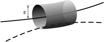
Figure 2: A diagonal line in a RP corresponds with a section of a trajectory (dashed) which stays within an $\varepsilon$-tube around another section (solid).

The most important numerical invariant related to the orbit growth is the topological entropy $h_{D}$. It represents the exponential growth rate for the number of orbit segments distinguishable with arbitrarily fine but finite precision. The topological entropy $h_{D}$ describes, roughly speaking, the total exponential complexity of the orbit structure with a single number. We just present the discrete case here (see also [19]).

Let $F:\mathcal{X}\rightarrow\mathcal{X}$ be a continuous map of a compact metric space $X$ with distance function $D$. We define an increasing sequence of metrics $D^{F}_{n},\;n=1,2,3,\ldots$, starting from $D^{F}_{1}=D$ by

$$D^{F}_{n}(x,y)=\max_{0\leq i\leq n-1}D\left(F^{i}(x),F^{i}(y)\right).$$ (4)

In other words, $D^{F}_{n}$ measures the distance between the orbit segments $I^{n}_{x}=\left\{x,\ldots,F^{n-1}x\right\}$ and $I^{n}_{y}=\left\{y,\ldots,F^{n-1}y\right\}$. We denote the open ball around $x$ by $B_{F}(x,\varepsilon,n)=\left\{y\in\mathcal{X}\mid D^{F}_{n}(x,y)<\varepsilon\right\}$.

A set $\mathcal{E}\subset\mathcal{X}$ is said to be $(n,\varepsilon)$-spanning if $\mathcal{X}\subset\bigcup_{x\in\mathcal{E}}B_{F}(x,\varepsilon,n)$. Let $S_{D}(F,\varepsilon,n)$ be the minimal cardinality of an $(n,\varepsilon)$-spanning set, or equivalently the cardinality of a minimal $(n,\varepsilon)$-spanning set. This quantity gives the minimal number of initial conditions whose behaviour approximates up to time $n$ the behaviour of any initial condition up to $\varepsilon$. Consider the exponential growth rate for that quantity

$$h_{D}(F,\varepsilon)=\overline{\lim\limits_{n\to\infty}}\frac{1}{n}\log S_{D}(F,\varepsilon,n),$$ (5)

where $\overline{\lim\limits_{n\to\infty}}$ denotes the supremum limit. Note that $h_{D}(F,\varepsilon)$ does not decrease with $\varepsilon$. Hence, the topological entropy $h_{D}(F)$ is defined as

$$h_{D}(F)=\lim\limits_{\varepsilon\to 0}h_{D}(F,\varepsilon).$$ (6)

It has been shown that if $D^{\prime}$ is another metric on $X$, which defines the same topology as $D$, then $h_{D^{\prime}}(F)=h_{D}(F)$ and the topological entropy will be an invariant of topological conjugacy [19]. Roughly speaking, this shows that a change of the coordinate system does not change the entropy. This is highly relevant, as it suggests that some of the structures in RPs do not depend on the special choice of the metric. The entropy $h_{D}$ allows characterising of dynamical systems with respect to their “predictability”, e g., periodic systems are characterised by $h_{D}=0$. If the system becomes more irregular, $h_{D}$ increases. Chaotic systems typically yield $0<h_{D}<\infty$, whereas time series of stochastic systems have infinite $h_{D}$.

Recurrences are furthermore related to UPOs and the topology of the attractor [42]. In Subsec. 3.11 we will describe this relationship in detail.

These considerations show that recurrences are deeply rooted in the theory of dynamical systems. Much of the efforts have been dedicated to the study of recurrence times. Additionally, in the late 1980’s Eckmann et al. have introduced RPs and the recurrence matrix. This matrix contains much information about the underlying dynamical system and can be exploited for the analysis of measured time series. Much of this report is devoted to the analysis of time series based on this matrix. We show how these methods are linked to theoretical concepts and show their respective applications.

3 Methods

Now we will use the concept of recurrence for the analysis of data and to study dynamical systems. Nonlinear data analysis is based on the study of phase space trajectories. At first, we introduce the concept of phase space reconstruction (Subsec. 3.1) and then give a technical and brief historical review on recurrence plots (Subsec. 3.2). This part is followed by the bivariate extension to cross recurrence plots (Subsec. 3.3) and the multivariate extension to joint recurrence plots (Subsec. 3.4). Then we describe measures of complexity based on recurrence/cross recurrence plots (Subsec. 3.5) and how dynamical invariants can be derived from RPs (Subsec. 3.6). Moreover, the potential of RPs for the analysis of spatial data, the detection of UPOs, detection and quantification of different kinds of synchronisation and the creation of surrogates to test for synchronisation is presented (Subsecs. 3.7–3.11). Before we describe several applications, we end the methodological section considering the influence of noise (Subsec. 3.12).

Most of the described methods and procedures are available in the CRP toolbox for Matlab^® (provided by TOCSY: http://tocsy.agnld.uni-potsdam.de).

3.1 Trajectories in phase space

The states of natural or technical systems typically change in time, sometimes in a rather intricate manner. The study of such complex dynamics is an important task in numerous scientific disciplines and their applications. Understanding, describing and forecasting such changes is of utmost importance for our daily life. The prediction of the weather, earthquakes or epileptic seizures are only three out of many examples.

Formally, a dynamical system is given by (1) a (phase) space (2) a continuous or discrete time and (3) a time-evolution law. The elements or “points” of the phase space represent possible states of the system. Let us assume that the state of such a system at a fixed time $t$ can be specified by $d$ components (e. g., in the case of a harmonic oscillator, these components could be its position and velocity). These parameters can be considered to form a vector

$$\vec{x}(t)=\left(x_{1}(t),\,x_{2}(t),\ldots,\,x_{d}(t)\right)^{\text{T}}$$ (7)

in the $d$-dimensional phase space of the system. In the most general setting, the time-evolution law is a rule that allows determining the state of the system at each moment of time $t$ from its states at all previous times. Thus the most general time-evolution law is time dependent and has infinite memory. However, we will restrict to time-evolution laws which enable calculating all future states given a state at any particular moment. For time-continuous systems the time evolution is given by a set of differential equations

$$\dot{\vec{x}}(t)=\frac{d\vec{x}(t)}{dt}=\vec{F}(\vec{x}(t)),\quad F:\mathds{R}^{d}\rightarrow\mathds{R}^{d}.$$ (8)

The vectors $\vec{x}(t)$ define a trajectory in phase space.

In experimental settings, typically not all relevant components to construct the state vector are known or cannot be measured. Often we are confronted with a time-discrete measurement of only one observable. This yields a scalar and discrete time series $u_{i}=u(i\Delta t)$, where $i=1,\ldots,N$ and $\Delta t$ is the sampling rate of the measurement. In such a case, the phase space has to be reconstructed [43, 44]. A frequently used method for the reconstruction is the time delay method:

$$\hat{\vec{x}}_{i}=\sum_{j=1}^{m}u_{i+(j-1)\tau}\,\vec{e}_{j},$$ (9)

where $m$ is the embedding dimension and $\tau$ is the time delay. The vectors $\vec{e}_{i}$ are unit vectors and span an orthogonal coordinate system ($\vec{e}_{i}\cdot\vec{e}_{j}=\delta_{i,j}$). If $m\geq 2D_{2}+1$, where $D_{2}$ is the correlation dimension of the attractor, Takens’ theorem and several extensions of it, guarantee the existence of a diffeomorphism between the original and the reconstructed attractor [44, 45]. This means that both attractors can be considered to represent the same dynamical system in different coordinate systems.

For the analysis of time series, both embedding parameters, the dimension $m$ and the delay $\tau$, have to be chosen appropriately. Different approaches for the estimation of the smallest sufficient embedding dimension (e. g. the false nearest neighbours algorithm [46]), as well as for an appropriate time delay $\tau$ (e. g. the auto-correlation function, the mutual information function; cf. [47, 46]) have been proposed.

Recurrences take place in a systems phase space. In order to analyse (univariate) time series by RPs, Eq. (1), we will reconstruct in the following the phase space by delay embedding, if not stated otherwise.

3.2 Recurrence plot (RP)

3.2.1 Definition

As our focus is on recurrences of states of a dynamical system, we define now the tool which measures recurrences of a trajectory $\vec{x}_{i}\in\mathds{R}^{d}$ in phase space: the recurrence plot, Eq. (1) [2]. The RP efficiently visualises recurrences (Fig. 3A) and can be formally expressed by the matrix

$$\mathbf{R}_{i,j}(\varepsilon)=\Theta\left(\varepsilon-\left\|\vec{x}_{i}-\vec{x}_{j}\right\|\right),\quad i,j=1,\ldots,N,$$ (10)

where $N$ is the number of measured points $\vec{x}_{i}$, $\varepsilon$ is a threshold distance, $\Theta(\cdot)$ the Heaviside function (i. e. $\Theta(x)=0$, if $x<0$, and $\Theta(x)=1$ otherwise) and $\left\|\cdot\right\|$ is a norm. For $\varepsilon$-recurrent states, i. e. for states which are in an $\varepsilon$-neighbourhood, we introduce the following notion

$$\vec{x}_{i}\approx\vec{x}_{j}\quad\Longleftrightarrow\quad\mathbf{R}_{i,j}\equiv 1.$$ (11)

The recurrence plot (RP) is obtained by plotting the recurrence matrix, Eq. (10), and using different colours for its binary entries, e. g., plotting a black dot at the coordinates $(i,j)$, if $\mathbf{R}_{i,j}\equiv 1$, and a white dot, if $\mathbf{R}_{i,j}\equiv 0$. Both axes of the RP are time axes and show rightwards and upwards (convention). Since $\mathbf{R}_{i,i}\equiv 1\,|_{i=1}^{N}$ by definition, the RP has always a black main diagonal line, the line of identity (LOI). Furthermore, the RP is symmetric by definition with respect to the main diagonal, i. e. $\mathbf{R}_{i,j}\equiv\mathbf{R}_{j,i}$ (see Fig. 3).

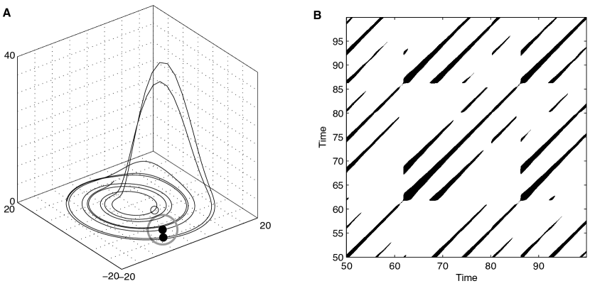
Figure 3: (A) Segment of the phase space trajectory of the Rössler system, Eqs. (• ‣ A), with $a=0.15$, $b=0.20$, $c=10$, by using its three components and (B) its corresponding recurrence plot. A phase space vector at $j$ which falls into the neighbourhood (grey circle in (A)) of a given phase space vector at $i$ is considered as a recurrence point (black point on the trajectory in (A)). This is marked with a black point in the RP at the position $(i,j)$. A phase space vector outside the neighbourhood (empty circle in (A)) leads to a white point in the RP. The radius of the neighbourhood for the RP is $\varepsilon=5$; $L_{2}$-norm is used.

In order to compute an RP, an appropriate norm has to be chosen. The most frequently used norms are the $L_{1}$-norm, the $L_{2}$-norm (Euclidean norm) and the $L_{\infty}$-norm (Maximum or Supremum norm). Note that the neighbourhoods of these norms have different shapes (Fig. 4). Considering a fixed $\varepsilon$, the $L_{\infty}$-norm finds the most, the $L_{1}$-norm the least and the $L_{2}$-norm an intermediate amount of neighbours. To compute RPs, the $L_{\infty}$-norm is often applied, because it is computationally faster and allows to study some features in RPs analytically.

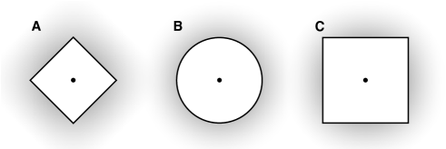
Figure 4: Three commonly used norms for the neighbourhood with the same radius around a point (black dot) exemplarily shown for the two-dimensional phase space: (A) $L_{1}$-norm, (B) $L_{2}$-norm and (C) $L_{\infty}$-norm.

3.2.2 Selection of the threshold $\varepsilon$

A crucial parameter of an RP is the threshold $\varepsilon$. Therefore, special attention has to be required for its choice. If $\varepsilon$ is chosen too small, there may be almost no recurrence points and we cannot learn anything about the recurrence structure of the underlying system. On the other hand, if $\varepsilon$ is chosen too large, almost every point is a neighbour of every other point, which leads to a lot of artefacts. A too large $\varepsilon$ includes also points into the neighbourhood which are simple consecutive points on the trajectory. This effect is called tangential motion and causes thicker and longer diagonal structures in the RP as they actually are. Hence, we have to find a compromise for the value of $\varepsilon$. Moreover, the influence of noise can entail choosing a larger threshold, because noise would distort any existing structure in the RP. At a higher threshold, this structure may be preserved (see Subsec. 3.12).

Several “rules of thumb” for the choice of the threshold $\varepsilon$ have been advocated in the literature, e. g., a few per cent of the maximum phase space diameter has been suggested [48]. Furthermore, it should not exceed 10% of the mean or the maximum phase space diameter [49, 50].

A further possibility is to choose $\varepsilon$ according to the recurrence point density of the RP by seeking a scaling region in the recurrence point density [51]. However, this may not be suitable for non-stationary data. For this case it was proposed to choose $\varepsilon$ such that the recurrence point density is approximately 1% [51].

Another criterion for the choice of $\varepsilon$ takes into account that a measurement of a process is a composition of the real signal and some observational noise with standard deviation $\sigma$ [52]. In order to get similar results as for the noise-free situation, $\varepsilon$ has to be chosen such that it is five times larger than the standard deviation of the observational noise, i. e. $\varepsilon>5\,\sigma$ (cf. Subsec. 3.12). This criterion holds for a wide class of processes.

For (quasi-)periodic processes, the diagonal structures within the RP can be used in order to determine an optimal threshold [53]. For this purpose, the density distribution of recurrence points along the diagonals parallel to the LOI is considered (which corresponds to the diagonal-wise defined $\tau$-recurrence rate $RR_{\tau}$, Eq. (50)). From such a density plot, the number of significant peaks $N_{\text{p}}$ is counted. Next, the average number of neighbours $N_{\text{n}}$, Eq. (44), that each point has, is computed. The threshold $\varepsilon$ should be chosen in such a way that $N_{p}$ is maximal and $N_{\text{n}}$ approaches $N_{\text{p}}$. Therefore, a good choice of $\varepsilon$ would be to minimise the quantity

$$\beta(\varepsilon)=\frac{|N_{\text{n}}(\varepsilon)-N_{\text{p}}(\varepsilon)|}{N_{\text{n}}(\varepsilon)}.$$ (12)

This criterion minimises the fragmentation and thickness of the diagonal lines with respect to the threshold, which can be useful for de-noising, e. g., of acoustic signals. However, this choice of $\varepsilon$ may not preserve the important distribution of the diagonal lines in the RP if observational noise is present (the estimated threshold can be underestimated).

Other approaches use a fixed recurrence point density. In order to find an $\varepsilon$ which corresponds to a fixed recurrence point density $RR$ (or recurrence rate, Eq. (41)), the cumulative distribution of the $N^{2}$ distances between each pair of vectors $P_{c}(D)$ can be used. The $RR^{\text{th}}$ percentile is then the requested $\varepsilon$ (e. g. for $RR=0.1$ the threshold $\varepsilon$ is given by $\varepsilon=D$ with $P_{c}(D)=0.1$). An alternative is to fix the number of neighbours for every point of the trajectory. In this case, the threshold is actually different for each point of the trajectory, i. e. $\varepsilon=\varepsilon(\vec{x}_{i})=\varepsilon_{i}$ (cf. Subsec. 3.2.5). The advantage of the latter two methods is that both of them preserve the recurrence point density and allow to compare RPs of different systems without the necessity of normalising the time series beforehand.

The choice of $\varepsilon$ depends strongly on the considered system under study. However, all kinds of dynamical invariants derived from RPs (cf. Subsec. 3.6) can only be obtained in the limit $\varepsilon\rightarrow 0$.

3.2.3 Structures in RPs

As already mentioned, the initial purpose of RPs was to provide a visual inspection of trajectories especially in a higher dimensional phase space. RPs yield important insights into the time evolution of these trajectories, because typical patterns in RPs are linked to a specific behaviour of the system. Large scale patterns in RPs, designated in [2] as typology, can be classified in homogeneous, periodic, drift and disrupted ones [2, 54]:

• Homogeneous RPs are typical of stationary systems in which the relaxation times are short in comparison with the time spanned by the RP. An example of such an RP is that of a stationary random time series (Fig. 5A).

• Periodic and quasi-periodic systems have RPs with diagonal oriented, periodic or quasi-periodic recurrent structures (diagonal lines, checkerboard structures). Fig. 5B shows the RP of a periodic system with two harmonic frequencies and with a frequency ratio of four (two and four short lines lie between the continuous diagonal lines). Irrational frequency ratios cause more complex quasi-periodic recurrent structures (the distances between the diagonal lines are different). However, even for oscillating systems whose oscillations are not easily recognisable, RPs can be useful (cf. unstable periodic orbits, Subsec. 3.11).

• A drift is caused by systems with slowly varying parameters, i. e. non-stationary systems. The RP pales away from the LOI (Fig. 5C).

• Abrupt changes in the dynamics as well as extreme events cause white areas or bands in the RP (Fig. 5D). RPs allow finding and assessing extreme and rare events easily by using the frequency of their recurrences.

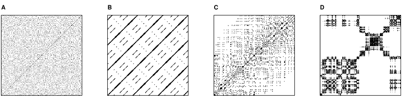
Figure 5: Characteristic typology of recurrence plots: (A) homogeneous (uniformly distributed white noise), (B) periodic (super-positioned harmonic oscillations), (C) drift (logistic map corrupted with a linearly increasing term $x_{i+1}=4x_{i}(1-x_{i})+0.01\,i$, cf. Fig. 23D) and (D) disrupted (Brownian motion). These examples illustrate how different RPs can be. The used data have the length 400 (A, B, D) and 150 (C), respectively; RP parameters are $m=1$, $\varepsilon=0.2$ (A, C, D) and $m=4$, $\tau=9$, $\varepsilon=0.4$ (B); $L_{2}$-norm.

A closer inspection of the RPs reveals also small-scale structures, the texture [2], which can be typically classified in single dots, diagonal lines as well as vertical and horizontal lines (the combination of vertical and horizontal lines obviously forms rectangular clusters of recurrence points); in addition, even bowed lines may occur [2, 54]:

• Single, isolated recurrence points can occur if states are rare, if they persist only for a very short time, or fluctuate strongly. However, they are not a unique sign of randomness or noise (e. g. in maps).

• A diagonal line $\mathbf{R}_{i+k,j+k}\equiv 1\,|_{k=0}^{l-1}$ (where $l$ is the length of the diagonal line) occurs when a segment of the trajectory runs almost in parallel to another segment (i. e. through an $\varepsilon$-tube around the other segment, Fig. 2) for $l$ time units:

  $$\vec{x}_{i}\approx\vec{x}_{j},\ \vec{x}_{i+1}\approx\vec{x}_{j+1},\ \ldots\,,\ \vec{x}_{i+l-1}\approx\vec{x}_{j+l-1}.$$ (13)

  A diagonal line of length $l$ is then defined by

  $$\left(1-\mathbf{R}_{i-1,j-1}\right)\left(1-\mathbf{R}_{i+l,j+l}\right)\prod_{k=0}^{l-1}\mathbf{R}_{i+k,j+k}\equiv 1.$$ (14)

  The length of this diagonal line is determined by the duration of such similar local evolution of the trajectory segments. The direction of these diagonal structures is parallel to the LOI (slope one, angle $\pi/4$). They represent trajectories which evolve through the same $\varepsilon$-tube for a certain time. Since the definition of the Rényi entropy of second order $K_{2}$ uses the time how long trajectories evolve in an $\varepsilon$-tube, the existence of a relationship between the length of the diagonal lines and $K_{2}$ (and even the sum of the positive Lyapunov exponents, Eq. (67)) is plausible (cf. invariants, Subsec. 3.6). Note that there might be also diagonal structures perpendicular to the LOI, representing parallel segments of the trajectory running with opposite time directions, i. e. $\vec{x}_{i}\approx\vec{x}_{j},\vec{x}_{i+1}\approx\vec{x}_{j-1},\ldots$ (mirrored segments). This is often a hint for an inappropriate embedding.

• A vertical (horizontal) line $\mathbf{R}_{i,j+k}\equiv 1\,|_{k=0}^{v-1}$ (with $v$ the length of the vertical line) marks a time interval in which a state does not change or changes very slowly:

  $$\vec{x}_{i}\approx\vec{x}_{j},\ \vec{x}_{i}\approx\vec{x}_{j+1},\ \ldots\,,\ \vec{x}_{i}\approx\vec{x}_{j+v-1}.$$ (15)

  The formal definition of a vertical line is

  $$\left(1-\mathbf{R}_{i,j-1}\right)\left(1-\mathbf{R}_{i,j+v}\right)\prod_{k=0}^{v-1}\mathbf{R}_{i,j+k}\equiv 1.$$ (16)

  Hence, the state is trapped for some time. This is a typical behaviour of laminar states (intermittency) [14].

• Bowed lines are lines with a non-constant slope. The shape of a bowed line depends on the local time relationship between the corresponding close trajectory segments (cf. Eq. (17)).

Diagonal and vertical lines are the base for a quantitative analysis of RPs (cf. Subsec. 3.5).

More generally, the line structures in RPs exhibit locally the time relationship between the current close trajectory segments [55]. A line structure in an RP of length $l$ corresponds to the closeness of the segment $\vec{x}(T_{1}(t))$ to another segment $\vec{x}(T_{2}(t))$, where $T_{1}(t)$ and $T_{2}(t)$ are two local and in general different time scales which preserves $\vec{x}(T_{1}(t))\approx\vec{x}(T_{2}(t))$ for some (absolute) time $t=1,\dots,l$. Under some assumptions (e. g., piece-wise existence of an inverse of the transformation $T(t)$, the two segments visit the same area in the phase space), a line in the RP can simply be expressed by the time-transfer function (Fig. 6)

$$\vartheta(t)=T_{2}^{-1}\left(T_{1}(t)\right).$$ (17)

Particularly, we find that the local slope $b(t)$ of a line in an RP represents the local time derivative of the inverse second time scale $T_{2}^{-1}(t)$ applied to the first time scale $T_{1}(t)$

$$b(t)=\partial_{t}T_{2}^{-1}\left(T_{1}(t)\right)=\partial_{t}\vartheta(t).$$ (18)

This is a fundamental relation between the local slope $b(t)$ of line structures in an RP and the time scaling of the corresponding trajectory segments. As special cases, we find that the slope $b=1$ (diagonal lines) corresponds to $T_{1}=T_{2}$, whereas $b=\infty$ (vertical lines) corresponds to $T_{2}\rightarrow 0$, i. e. the second trajectory segment evolves infinitely slow through the $\varepsilon$-tube around first trajectory segment. From the slope $b(t)$ of a line in an RP we can infer the relation $\vartheta(t)$ between two segments of $\vec{x}(t)$ ($\vartheta(t)=\int b(t)dt$). Note that the slope $b(t)$ depends only on the transformation of the time scale and is independent of the considered trajectory $\vec{x}(t)$ [55].

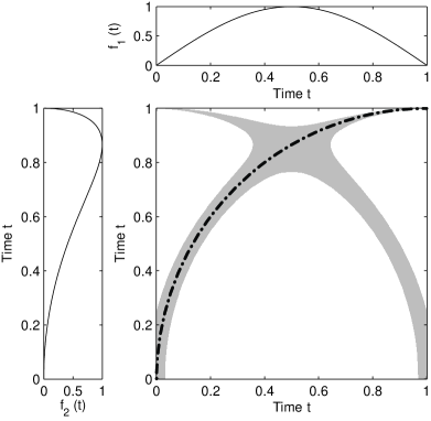
Figure 6: Detail of a recurrence plot for a trajectory $f(t)=\sin(\pi\,t)$ whose sub-sections $f_{1}(t)$ and $f_{2}(t)$ undergo different transformations in the time scale: $T_{1}(t)=t$ and $T_{2}(t)=1-\sqrt{1-t^{2}}$. The resulting bowed line (dash-dotted line) has the slope $b(t)=\frac{1-t}{\sqrt{1-(1-t)^{2}}}$, which corresponds with a segment of a circle.

This feature is, e. g., used in the application of CRPs as a tool for the adjustment of time scales of two data series [56, 55] and will be discussed in Subsec. 3.3.

Summarising the explanations about typology and texture, we establish the following list of features and give the corresponding qualitative interpretation (Tab. 1).

Table 1: Typical patterns in RPs and their meanings.

	Pattern	Meaning
(1)	Homogeneity	the process is stationary
(2)	Fading to the upper left and lower right corners	non-stationary data; the process contains a trend or a drift
(3)	Disruptions (white bands)	non-stationary data; some states are rare or far from the normal; transitions may have occurred
(4)	Periodic/quasi-periodic patterns	cyclicities in the process; the time distance between periodic patterns (e. g. lines) corresponds to the period; different distances between long diagonal lines reveal quasi-periodic processes
(5)	Single isolated points	strong fluctuation in the process; if only single isolated points occur, the process may be an uncorrelated random or even anti-correlated process
(6)	Diagonal lines (parallel to the LOI)	the evolution of states is similar at different epochs; the process could be deterministic; if these diagonal lines occur beside single isolated points, the process could be chaotic (if these diagonal lines are periodic, unstable periodic orbits can be observed)
(7)	Diagonal lines (orthogonal to the LOI)	the evolution of states is similar at different times but with reverse time; sometimes this is an indication for an insufficient embedding
(8)	vertical and horizontal lines/clusters	some states do not change or change slowly for some time; indication for laminar states
(9)	Long bowed line structures	the evolution of states is similar at different epochs but with different velocity; the dynamics of the system could be changing

Another problem is the LOI; some authors exclude it from the RP. This may be useful for the quantification of RPs, which we will discuss later. It can also be motivated by the definition of the Grassberger-Procaccia correlation sum [57] (or generalised 2${}^{\text{nd}}$ order correlation integral) which was introduced for the determination of the correlation dimension $D_{2}$ and is closely related to RPs:

$$C_{2}(\varepsilon)=\frac{1}{N^{2}}\sum_{\begin{subarray}{c}i,j=1\\ i\not=j\end{subarray}}^{N}\Theta\left(\varepsilon-\left\|\vec{x}_{i}-\vec{x}_{j}\right\|\right),\qquad\vec{x}\in\mathds{R}^{d}.$$ (19)

Eq. (19) excludes the comparisons of $\vec{x}_{i}$ with itself. Nevertheless, since the threshold value $\varepsilon$ is finite (and normally about $10$% of the mean phase space radius), further long diagonal lines can occur directly below and above the LOI for smooth or high resolution data. Therefore, the diagonal lines in a small corridor around the LOI correspond to the tangential motion of the phase space trajectory, but not to different orbits. Thus, for the estimation of invariants of the dynamical system, it is better to exclude this entire corridor and not only the LOI. This step corresponds to suggestions to exclude the tangential motion as it is done for the computation of the correlation dimension (known as Theiler correction or Theiler window [58]) or for the alternative estimators of Lyapunov exponents [59, 60] in which only those phase space points are considered that fulfil the constraint $|j-i|\geq w$. Theiler has suggested using the auto-correlation time as an appropriate value for $w$ [58], and Gao and Zheng state that $w=(m-1)\tau$ would be sufficient [60]. However, in a representation of an RP it is better to picture the LOI. This LOI has also importance when applications of cross recurrence plots will be discussed (Sec. 4.4).

The visual interpretation of RPs requires some experience. RPs for paradigmatic systems provide an instructive introduction into characteristic typology and texture (e. g. Fig. 5). However, a quantification of the obtained structures is necessary for a more objective investigation of the considered system (see Subsec. 3.5).

The previous statements hold for systems, whose characteristic frequencies are much lower than the sampling frequency of their observation. If the sampling frequency is only one magnitude higher than the system’s frequencies, and their ratio is not a multiple of an integer, and consequently some recurrences will not be found although they should be there [61]. This discretisation effect yields in extended characteristic gaps in the recurrence plot, those appearances depend on the modulations of the systems frequencies (Fig. 7).

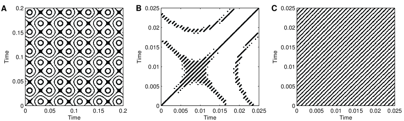
Figure 7: (A) Characteristic patterns of gaps (all white areas) in a recurrence plot of a modulated harmonic oscillation $\cos(2\pi 1000t+0.5\sin(2\pi 25t))$, which is sampled with a sampling frequency of 1 kHz. (B) Magnified detail of the RP presented in (A), which obtains the actual periodic line structure due to the oscillation, but disturbed by extended white areas. (C) Corresponding RP as shown in (B), but for a higher sampling rate of 10 kHz. The periodic line structure due to the oscillation covers now the entire RP. Used RP parameters: $m=3$, $\tau=1$, $\varepsilon=0.05\sigma$, $L_{\infty}$-norm.

3.2.4 Influence of embedding on the structures in RPs

In the case that only a scalar time series has been measured, the phase space has to be reconstructed, e. g., by means of the delay embedding technique. However, the embedding can cause a considerable amount of spurious correlations in the regarded system, which are then reflected in the RP (Fig. 8). This effect can even yield distinct diagonally oriented structures in an RP of a time series of uncorrelated values if the embedding is high, although diagonal structures should be extremely rare for such uncorrelated data.

Figure 8: Correlation between a single recurrence point at $(15,30)$ (marked with grey circle) and other recurrence points in an RP for an uncorrelated Gaussian noise (estimated from 2,000 realisations). The embedding parameters are (A) $m=1$, $\tau=1$, $\varepsilon=0.38$, (B) $m=3$, $\tau=5$, $\varepsilon=1.22$ and (C) $m=5$, $\tau=2$, $\varepsilon=1.62$, which preserve an approximately constant recurrence point density (0.2).

In order to understand this, we consider uncorrelated Gaussian noise $\xi_{i}$ with standard deviation $\sigma$ and compute analytically correlations that are induced by a non-appropriate embedding. Because the considered process is uncorrelated, the correlations detected afterwards must be due to the method of embedding.

Using time delay embedding, Eq. (9), with embedding dimension $m$ and delay $\tau$, a vector in the reconstructed phase space is given by

$$\vec{x}_{i}=\sum\limits_{k=0}^{m-1}\xi_{i+k\tau}\vec{e}_{k}.$$ (20)

The distance between each pair of these vectors is $\mathbf{D}_{i,j}=\left\|\vec{x}_{i}-\vec{x}_{j}\right\|$. Moving $h$ steps ahead in time (i. e. along a diagonal line in the RP) the respective distance is $\mathbf{D}_{i+h,j+h}=\left\|\vec{x}_{i+h}-\vec{x}_{j+h}\right\|$. For convenience, the auto-covariance function of $\mathbf{D}_{i,j}^{2}$ will be computed instead of computing the auto-covariance function of $\mathbf{D}_{i,j}$. Using the $L_{2}$-norm, the auto-covariance function is

$$\mathrm{cov}_{\mathbf{D}^{2}}(h,j-i) = \left<\left(\sum\limits_{k=0}^{m-1}\left(\xi_{i+k\tau}-\xi_{j+k\tau}\right)^{2}-E\right)\right.$$ (21)

$$\left.\left(\sum\limits_{k=0}^{m-1}\left(\xi_{i+h+k\tau}-\xi_{j+h+k\tau}\right)^{2}-E\right)\right>,$$

where

$$E=\left<\sum\limits_{k=0}^{m-1}\left(\xi_{i+k\tau}-\xi_{j+k\tau}\right)^{2}\right>=2\sigma^{2}m\left(1-\delta_{0,j-i}\right)$$ (22)

is the expectation value and $\delta_{i,j}$ is the Kronecker delta ($\delta_{i,j}=1$ if $i=j$, and $\delta_{i,j}=0$ if $i\neq j$). Setting $p=j-i$ and assuming $p>0$ and $h>0$ to avoid trivial cases, we find [62]

$$\mathrm{cov}_{\mathbf{D}^{2}}(h,p)=\sum\limits_{k=0}^{m-1}(m-k)\left(8\delta_{k\tau,h}+2\delta_{k\tau,p+h}+\delta_{k\tau,p-h}\right).$$ (23)

This equation shows that there will be peaks in the auto-covariance function if $h$, $p+h$ or $p-h$ are equal to one of the first $m-1$ multiples of $\tau$. These peaks are not present when no embedding is used ($m=1$). Such spurious correlations induced by embedding lead to modified small-scale structures in the RP: an increase of the embedding dimension cleans up the RP from single recurrence points (representatives for the uncorrelated states) and emphasises the diagonal structures as diagonal lines (representatives for the correlated states). This, of course, influences any quantification of RPs, which is based on diagonal lines. Hence, we should be careful in interpreting and quantifying structures in RPs of measured systems. If the embedding dimension is, e. g., inappropriately high, spurious long diagonal lines will appear in the RP. In order to avoid this problem, the embedding parameters have to be chosen carefully, or alternatively quantification measures which are independent of the embedding dimension have to be used (cf. Subsec. 3.6).

The spurious correlations in RPs due to embedding can also be understood from the fact that an RP computed with any embedding dimension can be derived from an RP computed without embedding ($m=1$). Consider, e. g., $m=2$ with certain $\tau$ and the maximum norm. A recurrence point at $(i,j)$ will occur if

$$\vec{x}_{i}\approx\vec{x}_{j}\quad\Longleftrightarrow\quad\max\left(|x_{i}-x_{j}|,|x_{i+\tau}-x_{j+\tau}|\right)<\varepsilon.$$ (24)

This is the same as $x_{i}\approx x_{j}$ and $x_{i+\tau}\approx x_{j+\tau}$ and corresponds to two recurrence points at $(i,j)$ and $(i+\tau,j+\tau)$ in an RP without embedding. Thus, a recurrence point for a reconstructed trajectory with an embedding dimension $m$ is

$$\mathbf{R}_{i,j}^{(m)}=\mathbf{R}_{i,j}^{(1)}\cdot\mathbf{R}_{i+\tau,j+\tau}^{(1)}\cdot\ldots\cdot\mathbf{R}_{i+(m-1)\tau,j+(m-1)\tau}^{(1)},$$ (25)

where $\mathbf{R}^{(1)}$ is the RP without embedding (or parent RP) and $\mathbf{R}^{(m)}$ is the RP for embedding dimension $m$ [8]. The entry at $(i,j)$ in the recurrence matrix $\mathbf{R}^{(m)}$ consists of information at times $(i+\tau,j+\tau),\ldots,(i+(m-1)\tau,j+(m-1)\tau)$. If the threshold $\varepsilon$ is large enough, spurious recurrence points along the line $(i+k,j+k)$ for $k=0\,\ldots,(m-1)\tau$ can appear. It is clear that, e. g., in the case of a stochastic signal which is embedded in a high-dimensional space, such diagonal lines in an RP may feign a non-existing determinism.

3.2.5 Modifications and extensions

In the original definition of RPs, the neighbourhood is a ball (i. e. $L_{2}$-norm is used) and its radius is chosen in such a way that it contains a fixed amount $N_{\text{n}}$ of states $\vec{x}_{j}$ [2]. With such a neighbourhood, the radius $\varepsilon=\varepsilon_{i}$ changes for each $\vec{x}_{i}$ and $\mathbf{R}_{i,j}\not=\mathbf{R}_{j,i}$ because the neighbourhood of $\vec{x}_{i}$ is in general not the same as that of $\vec{x}_{j}$. This leads to an asymmetric RP, but all columns of the RP have the same recurrence density (Fig. 11D). Using this neighbourhood criterion, $\varepsilon_{i}$ can be adjusted in such a way that the recurrence point density has a fixed predetermined value (i. e. $RR=N_{\text{n}}/N$). This neighbourhood criterion is denoted as fixed amount of nearest neighbours (FAN). However, the most commonly used neighbourhood is that with a fixed radius $\varepsilon_{i}=\varepsilon,\forall i$. For RPs this neighbourhood was firstly used in [13]. A fixed radius means that $\mathbf{R}_{i,j}=\mathbf{R}_{j,i}$ resulting in a symmetric RP. The type of neighbourhood that should preferably be used depends on the purpose of the analysis. Especially for the later introduced cross recurrence plots (Subsec. 3.3) and the detection of generalised synchronisation (Subsec. 3.8.4), the neighbourhood with a FAN will play an important role.

In the literature further variations of RPs have been proposed (henceforth we assume $\vec{x}\in\mathds{R}^{d}$):

• Instead of plotting the recurrence matrix (Eq. 10), the distances

  $$\mathbf{D}_{i,j}=\|\vec{x}_{i}-\vec{x}_{j}\|$$ (26)

  can be plotted (Fig. 11H). Although this is not an RP, it is sometimes called global recurrence plot [63] or unthresholded recurrence plot [64]. The name distance plot would be perhaps more appropriate.

  A practical modification is the unthresholded recurrence plot defined in terms of the correlation sum $C_{2}$, Eq. (19),

  $$\mathbf{U}_{i,j}=C_{2}\left(\|\vec{x}_{i}-\vec{x}_{j}\|\right),$$ (27)

  where the values of the correlation sum with respect to the distance $\|\vec{x}_{i}-\vec{x}_{j}\|$ are used [8]. Applying a threshold $\varepsilon$ to such an unthresholded RP reveals an RP with a recurrence point density which is exactly $\varepsilon$.

  These representations can also help in studying phase space trajectories. Moreover, they may help to find an appropriate threshold value $\varepsilon$.

• Iwanski and Bradley defined a variation of an RP with a corridor threshold $[\varepsilon_{\text{in}},\varepsilon_{\text{out}}]$ (Fig. 11E) [64],

  $$\mathbf{R}_{i,j}([\varepsilon_{\text{in}},\,\varepsilon_{\text{out}}])=\Theta\left(\left\|\vec{x}_{i}-\vec{x}_{j}\right\|-\varepsilon_{\text{in}}\right)\cdot\Theta\left(\varepsilon_{\text{out}}-\left\|\vec{x}_{i}-\vec{x}_{j}\right\|\right).$$ (28)

  Those points $\vec{x}_{j}$ are considered to be recurrent that fall into the shell with the inner radius $\varepsilon_{\text{in}}$ and the outer radius $\varepsilon_{\text{out}}$. An advantage of such a corridor thresholded recurrence plot is its increased robustness against recurrence points coming from the tangential motion. However, the threshold corridor removes the inner points in broad diagonal lines, which results in two lines instead of one. These RPs are, therefore, not directly suitable for a quantification analysis. The shell as a neighbourhood was used in an attempt to compute Lyapunov exponents from experimental time series [65].

• Choi et al. introduced the perpendicular recurrence plot (Fig. 11F) [66]

  $$\mathbf{R}_{i,j}(\varepsilon)=\Theta\left(\varepsilon-\left\|\vec{x}_{i}-\vec{x}_{j}\right\|\right)\cdot\delta\left(\dot{\vec{x}}_{i}\cdot(\vec{x}_{i}-\vec{x}_{j})\right),$$ (29)

  with $\delta$ denoting the Delta function ($\delta(x)=1$ if $x=0$, and $\delta(x)=0$ otherwise). This RP contains only those points $\vec{x}_{j}$ that fall into the neighbourhood of $\vec{x}_{i}$ and lie in the $(d-1)$-dimensional subspace of $\mathds{R}^{d}$ that is perpendicular to the phase space trajectory at $\vec{x}_{i}$. These points correspond locally to those lying on a Poincaré section. This criterion cleans up the RP more effectively from recurrence points based on the tangential motion than the previous corridor thresholded RPs. This kind of RP is more efficient for estimating invariants and is more robust for the detection of UPOs (if they exist).

• The iso-directional recurrence plot, introduced by Horai and Aihara [67],

  $$\mathbf{R}_{i,j}(\varepsilon,T)=\Theta\left(\varepsilon-\left\|\left(\vec{x}_{i+T}-\vec{x}_{i}\right)-\left(\vec{x}_{j+T}-\vec{x}_{j}\right)\right\|\right),$$ (30)

  is another variant which takes the direction of the trajectory evolution into account. Here a recurrence is related to neighboured trajectories which run parallel and in the same direction. The authors introduced an additional iso-directional neighbours plot, which is simply the product between the common RP and the iso-directional RP [67]

  $$\mathbf{R}_{i,j}(\varepsilon,T)=\Theta\left(\varepsilon-\left\|\vec{x}_{i}-\vec{x}_{j}\right\|\right)\cdot\Theta\left(\varepsilon-\left\|\left(\vec{x}_{i+T}-\vec{x}_{i}\right)-\left(\vec{x}_{j+T}-\vec{x}_{j}\right)\right\|\right).$$ (31)

  The computation of this special recurrence plot is simpler than that of the perpendicular RP. Although the cleaning of the RP from false recurrences is better than in the common RP, it does not reach the quality of a perpendicular RP. A disadvantage is the additional parameter $T$ which has to be determined carefully in advance (however, it seems that this parameter can be related to the embedding delay $\tau$).

• It is also possible to test each state with a pre-defined amount $k$ of subsequent states [68, 13, 49]

  $$\mathbf{R}_{i,j}(\varepsilon)=\Theta\left(\varepsilon-\left\|\vec{x}_{i}-\vec{x}_{i+i_{0}+j-1}\right\|\right),\quad i=1,\ldots,N-k,\ j=1,\ldots,k.$$ (32)

  This reveals an $(N-k)\times k$-matrix which does not have to be square (Fig. 11J). The $y$-axis represents the time distances to the following recurrence points but not their absolute time. All diagonally oriented structures in the common RP are now projected to the horizontal direction. For $i_{0}=0$, the LOI, which was the main diagonal line in the original RP, is now the horizontal line which coincides with the $x$-axis. With non-zero $i_{0}$, the RP contains recurrences of a certain state only in the pre-defined time interval after time $i_{0}$ [49].

  This representation of recurrences may be more intuitive than that of the original RP because the consecutive states are not oriented diagonally. However, such an RP represents only the first $(N-k)$ states. Mindlin and Gilmore proposed the close returns plot [48] which is, in fact, such an RP exactly for dimension one. Using this definition of RP, a first quantification approach of RPs (or “close returns plots”) was introduced (“close returns histogram”, recurrence times; cf. Subsec. 3.5.2). It has been used for the investigation of periodic orbits and topological properties of strange attractors [69, 70, 48].

• The windowed and meta recurrence plots have been suggested as tools to investigate an external force or non-stationarity in a system [71, 72]. The first ones are obtained by covering an RP with $w\times w$-sized squares (windows) and by averaging the recurrence points that are contained in these windows [72]. Consequently, a windowed recurrence plot is an $N_{w}\times N_{w}$-matrix, where $N_{w}$ is the floor-rounded $N/w$, and consists of values which are not limited to zero and one (this suggests a colour-encoded representation). These values correspond to the cross correlation sum, Eq. (42),

  $$\mathbf{C}_{I,J}(\varepsilon)=\frac{1}{w^{2}}\sum_{i,j=1}^{w}\mathbf{R}_{i+(I-1)w,j+(J-1)w}(\varepsilon)\,,\quad I,J=1,\ldots,\frac{N}{w}$$ (33)

  between sections in $\vec{x}$ with length $w$ and starting at $(I-1)w+1$ and $(J-1)w+1$ (for cross correlation integral cf. [73]). Windowed RPs can be useful for the detection of transitions or large-scale patterns in RPs of very long data series.

  The meta recurrence plot, as defined in [72], is a distance matrix derived from the cross correlation sum, Eq. (33),

  $$\mathbf{D}_{I,J}(\varepsilon)=\frac{1}{\varepsilon^{d}}\left(\mathbf{C}_{I,I}(\varepsilon)+\mathbf{C}_{J,J}(\varepsilon)-2\,\mathbf{C}_{I,J}(\varepsilon)\right).$$ (34)

  By applying a further threshold value to $\mathbf{D}_{I,J}(\varepsilon)$ (analogous to Eq. (10)), a black-white dotted representation is also possible.

  Manuca and Savit have gone one step further by using quotients from the cross correlation sum to form a meta phase space [71]. From this meta phase space a recurrence or non-recurrence plot is created, which can be used to characterise non-stationarity in time series.

• Instead of using the spatial closeness between phase space trajectories, order patterns recurrence plots (OPRP) are based on order patterns $\pi$ for the definition of a recurrence. An order pattern $\pi$ of dimension $d$ is defined by the discrete order sequence of the data series $x_{i}$ and has the length $d$. For $d=3$ we get, e. g., six different order patterns (Fig. 9). Using these order patterns, the data series $x_{i}$ is symbolised by order patterns:

  $$x_{i},x_{i-\tau_{1}},\ldots,x_{i-\tau_{d}-1}\ \rightarrow\ \pi_{i}.$$

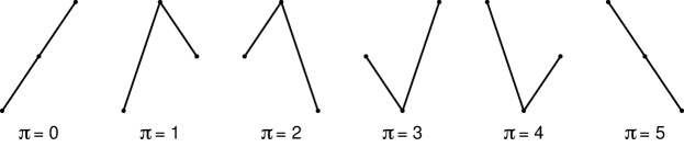
Figure 9: Order patterns for dimension $d=3$. They describe a specific rank order of three data points and can be used to exhibit a recurrence by means of local rank order sequence.

The order patterns recurrence plot (Fig. 11G) is then defined by the pair-wise test of order patterns [74]:

$$\mathbf{R}_{i,j}(d)=\delta\left(\pi_{i},\ \pi_{j}\right).$$ (35)

Such an RP represents those times, when specific rank order sequences in the system recur. Its main advantage is its robustness with respect to non-stationary data. Moreover, it increases the applicability of cross recurrence plots (cf. Subsec. 3.3).

A hybrid between a common RP and an OPRP is the ordinal recurrence plot (Fig. 11I) [75]:

$$\mathbf{R}_{i,j}(d) = \Theta\left(s(x_{i+\tau}-x_{i})\right)\Theta\left(s(x_{j+\tau}-x_{j})\right)\cdot$$ (36)

$${}\Theta\left(s(x_{i+\tau}-x_{j})\right)\Theta\left(s(x_{j+\tau}-x_{i})\right),\ \text{for}\ s\in\{-1,+1\}.$$

It looks whether two states are close and, additionally, whether such both states grow or shrink simultaneously (Fig. 10).

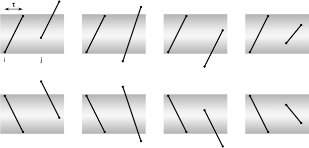
Figure 10: Ordinal cases which are considered to be a recurrence in an ordinal recurrence plot.

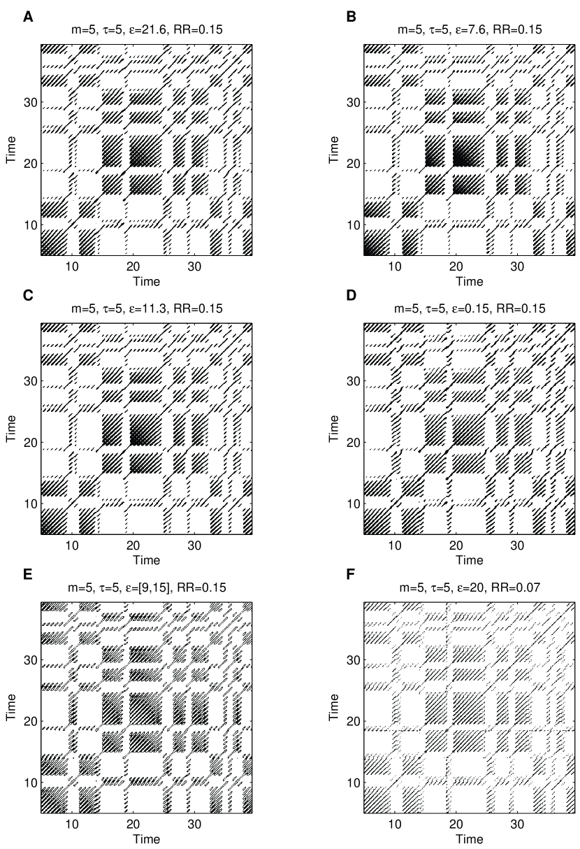
Figure 11: Continued on p. 11.

Furthermore, the term recurrent plots can be found for RPs in the literature (e. g. [76]). However, this term should not be used for RPs (it is sometimes used for return time plots). Finally, it should be mentioned that the term recurrence plots is sometimes used for another representation not related to RPs (e. g. [77]).

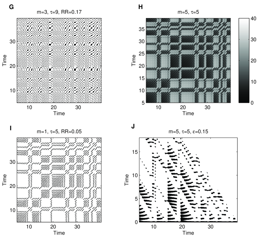
Figure 11: Examples of various definitions of RPs for a section of the $x$-component of the Lorenz system, Eqs. (• ‣ A), $r=28$, $\sigma=10$, $b=\frac{8}{3}$, sampling time $\Delta t=0.03$ [78]: (A) RP by using the $L_{\infty}$-norm, (B) RP by using the $L_{1}$-norm, (C) RP by using the $L_{2}$-norm, (D) RP by using a fixed amount of nearest neighbours (FAN), (E) RP by using a threshold corridor $[\varepsilon_{\text{in}},\varepsilon_{\text{out}}]$, (F) perpendicular RP ($L_{2}$-norm), (G) order patterns RP ($m=3$, $\tau_{1,\,2,\,3}=9$), (H) distance plot (unthresholded RP, $L_{2}$-norm), (I) ordinal RP ($m=1$, $\tau=5$), (J) RP where the $y$-axis represents the relative time distances to the next recurrence points but not their absolute time (“close returns plot”, $L_{2}$-norm). Except for (F), (G), (H) and (I), the parameter $\varepsilon$ is chosen in such a way that the recurrence point density (RR) is approximately the same. The embedding parameters ($m=5$ and $\tau=5$) correspond to an appropriate time delay embedding.

The selection of a specific definition of the RP depends on the problem and on the kind of system or data. Perpendicular RPs are highly recommended for the quantification analysis based on diagonal structures, whereas corridor thresholded RPs are not suitable for this task. Windowed RPs are appropriate for the visualisation of the long-range behaviour of rather long data sets. If the recurrence behaviour for the states $\vec{x}_{i}$ within a pre-defined section $\{\vec{x}_{i+i_{0}},\,\ldots,\,\vec{x}_{i+i_{0}+k}\}$ of the phase space trajectory is of special interest, an RP with a horizontal LOI will be suitable. We will use the standard definition of RP, Eq. (10), according to [2] in this report.

It should be emphasised again that the recurrence of states is a fundamental concept in the analysis of dynamical systems. Besides RPs, there are some other methods that use recurrences: e. g. recurrence time statistics [41, 34, 79], first return map [69], space time separation plot [80] or recurrence based measures for the detection of non-stationarity (closely related to the recurrence time statistics, [81, 82]).

The pair-wise test between all elements of a series or of two different series, can also be found in other methods much earlier than 1987. There are some methods rather similar to RPs developed in several fields. To our knowledge, first ideas go back to the 70ies, where the dynamic time warping was developed for speech recognition. The purpose was to match or align two sequences [83, 84]. For a similar purpose, but for genome sequence alignment, the dot matrix, similarity plot or sequence matrix (several terms for the same thing) were introduced [e. g. 85, 86, 87]. Remarkable variations thereof are dot plots and link plots, which were developed to detect structures in text and computer codes [88], and similarity plots, developed for the analysis of changing images [89]. The self-similarity matrix and the ixegram represent similarities or distances of features in long data series, like frequencies, histograms or specific descriptors. They are used to recognise specific structures in music and the ixegram is part of the MPEG-7 standard [90, 91]. Contact maps are used to visualise the complex structures of folded proteins and to reconstruct them (e. g. by measuring the distances between C atoms) and go back to the early 70ies (e. g. [92, 93, 94]). We have already mentioned the close returns plots as a special case of the RPs for $m=1$, but they should be listed here too. They were introduced to recognise periodic orbits and topological properties of attractors and differ from RPs in the use of consecutive states as the $y$-axis instead of all states [48].

3.3 Cross recurrence plot (CRP)

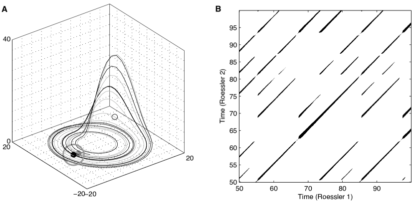
Figure 12: (A) Phase space trajectories of two coupled Rössler systems, Eqs. (• ‣ A) and (• ‣ A), with $a=0.15$, $b=0.20$, $c=10$, $\nu=0.015$ and $\mu=0.01$ by using their three components (black and grey line correspond to the first and second oscillator). In (B) the corresponding CRP is shown ($L_{2}$ norm and $\varepsilon=3$ is used). (A) If a phase space vector of the second Rössler system at $j$ (grey point on the grey line) falls into the neighbourhood (grey circle) of a phase space vector of the first Rössler system at $i$, in the CRP (B) at the location $(i,j)$ a black point will occur.

The cross recurrence plot (CRP) is a bivariate extension of the RP and was introduced to analyse the dependencies between two different systems by comparing their states [95, 96]. They can be considered as a generalisation of the linear cross-correlation function. Suppose we have two dynamical systems, each one represented by the trajectories $\vec{x}_{i}$ and $\vec{y}_{i}$ in a $d$-dimensional phase space (Fig. 12A). Analogously to the RP, Eq. (10), the corresponding cross recurrence matrix (Fig. 12B) is defined by

$$\mathbf{CR}^{\vec{x},\vec{y}}_{i,j}(\varepsilon)=\Theta\left(\varepsilon-\|\vec{x}_{i}-\vec{y}_{j}\|\right),\qquad i=1,\ldots,N,\ j=1,\ldots,M,$$ (37)

where the length of the trajectories of $\vec{x}$ and $\vec{y}$ is not required to be identical, and hence the matrix $\mathbf{CR}$ is not necessarily square. Note that both systems are represented in the same phase space, because a CRP looks for those times when a state of the first system recurs to one of the other system. Using experimental data, it is sometimes difficult to reconstruct the phase space. If the embedding parameters are estimated from both time series, but are not equal, the higher embedding should be chosen. However, the data under consideration should be from the same (or a very comparable) process and, actually, should represent the same observable. Therefore, the reconstructed phase space should be the same. An exception is the order patterns cross recurrence plot, where the values of the states are not directly compared but the local rank order sequence of the two systems [97]. Then both systems can be represented by different observables (or time series of very different amplitudes).

This bivariate extension of the RP was introduced for the cross recurrence quantification [95]. Independently, the concept of CRPs also surfaces in an approach to study interrelations between time series [98]. The components of $\vec{x}_{i}$ and $\vec{y}_{i}$ are usually normalised before computing the cross recurrence matrix. Other possibilities are to use a fixed amount of neighbours (FAN) for each $\vec{x}_{i}$ or to use order patterns [74]. This way the components of $\vec{x}_{i}$ and $\vec{y}_{i}$ do not need to be normalised. The latter choices of the neighbourhood have the additional advantage of working well for slowly changing trajectories (e. g. drift).

Since the values of the main diagonal $\mathbf{CR}_{i,i}\,|_{i=1}^{N}$ are not necessarily one, there is usually not a black main diagonal (Fig. 12B). Apart from that, the statements given in the subsection about all the structures in RPs (Subsec. 3.2.3, Tab. 1) hold also for CRPs. The lines which are diagonally oriented are here of major interest too. They represent segments on both trajectories, which run parallel for some time. The frequency and length of these lines are obviously related to a certain similarity between the dynamics of both systems. A measure based on the lengths of such lines can be used to find nonlinear interrelations between two systems (cf. Subsecs. 3.5 and  4.5), which cannot be detected by the common cross-correlation function [96].

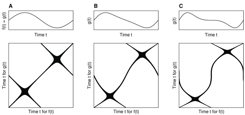
Figure 13: CRPs of sine functions $f(t)=\sin(\varphi t)$ and $g(t)=\sin(\varphi t+a\sin(\psi t))$ with fixed frequencies $\varphi$ and $\psi$, whereas (A) $a=0$, (B) $a=0.5$ and (C) $a=1$. The variation in the time domain leads to a deformation of the synchronisation line. The CRPs are computed without embedding.

An important advantage of CRPs is that they reveal the local difference of the dynamical evolution of close trajectory segments, represented by bowed lines. A time dilatation or time compression of one of the trajectories causes a distortion of the diagonal lines (cf. remarks about the relationship between the slope of RP lines and local time transformations in Subsec. 3.2.3). Assuming two identical trajectories, the CRP coincides with the RP of one trajectory and contains the main black diagonal or line of identity (LOI). If the values of the second trajectory are slightly modified, the LOI will become somewhat disrupted and is called line of synchronisation (LOS). However, if we do not modify the amplitudes but stretch or compress the second trajectory slightly, the LOS will still be continuous but not a straight line with slope one (angle of $\pi/4$). This line can rather become bowed (Fig. 13). As we have already seen in the Subsec. 3.2.3, the local slope of lines in an RP as well as in a CRP corresponds to the transformation of the time axes of the two considered trajectories, Eq. (18) [55]. A time shift between the trajectories causes a dislocation of the LOS. Hence, the LOS may lie rather far from the main diagonal of the CRP. As we will see in the following example, the LOS allows finding the non-parametric rescaling function between different time series.

Example: Time scale alignment of two harmonic functions with changing frequencies

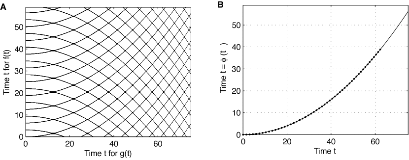
Figure 14: (A) Cross recurrence plot of two sine functions $f(t)=\sin(\varphi t)$ and $g(t)=\sin(\psi t^{2})$, which is the base for the determination of the rescaling function between both data series. The CRP was created without embedding and using FAN $\varepsilon=0.1$ (constant recurrence density of 10 %). (B) Time-transfer function (black) determined from the CRP. It has the expected parabolic shape of the squared coherence in the time domain (dotted line: square function).

We consider two sine functions $f(t)=\sin(\varphi t)$ and $g(t^{\prime})=\sin(\psi t^{\prime})=\sin(\psi t^{2})$, where the time scale of the second sine differs from the first by a quadratic transformation ($t^{\prime}=t^{2}$) and has a frequency of $\psi=0.01\,\varphi$. Such a nonlinear changing of time scales can be found in nature, e. g., with increasing depth, sediments in a lake undergo an increasing amount of pressure resulting in compression (cf. Subsec. 4.4). It can be assumed that both data series come from the same process and were subjected to different deposital compressions (e. g. a squared or exponential increasing of the compression). Hence, their CRP contains a bowed LOS (Fig. 14A). We have used no embedding and a varying threshold $\varepsilon$, such that the CRP contains a constant recurrence density of 10 % (FAN). In order to find the non-parametrical time-transfer function $t=\phi(t^{\prime})$, the LOS has to be resolved from the CRP. The resulting rescaling function has the expected squared shape $t=\phi(t^{\prime})=0.01\,t^{\prime 2}$ (grey dashed curve in Fig. 14B). Substituting the time scale $t^{\prime}$ in the second data series $g(t^{\prime})$ by this rescaling function $t=\phi(t^{\prime})$, we get a set of aligned data $f(t)$ and $g(t)$ with the non-parametric rescaling function $t=\phi(t^{\prime})$ (Fig. 15). The aligned data series are now approximately the same.

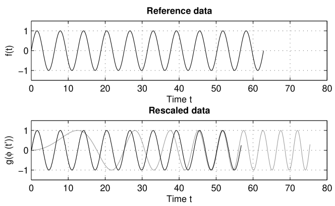
Figure 15: Reference data series (upper panel) and rescaled data series before (grey) and after (black) rescaling by using the time-transfer function presented in Fig. 14 (lower panel).

3.4 Joint recurrence plot (JRP)

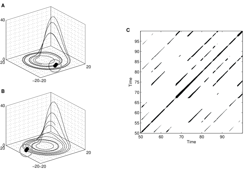
Figure 16: (A, B) Phase space trajectories of two coupled Rössler systems, Eqs. (• ‣ A) and (• ‣ A), with $a=0.15$, $b=0.20$, $c=10$, $\nu=0.015$ and $\mu=0.01$. In (C) the corresponding JRP is shown ($L_{2}$ norm and $\varepsilon=5$ is used for both systems). If two phase space vectors of the second Rössler system at $i$ and $j$ are neighbours (black points in (B)) and if two phase space vectors of the first Rössler system at same $i$ and $j$ are also neighbours (black points in (A)), a black point in the JRP at the location $(i,j)$ will occur.

As we have seen in the previous section, the bivariate extension of RPs to CRPs allows studying the relationship between two different systems by examining the occurrence of similar states. However, CRPs cannot be used for the analysis of two physically different time series, because the difference between two vectors with different physical units or even different phase space dimension does not make sense.

Another possibility to compare different systems is to consider the recurrences of their trajectories in their respective phase spaces separately and look for the times when both of them recur simultaneously, i. e. when a joint recurrence occurs. By means of this approach, the individual phase spaces of both systems are preserved. Formally, this corresponds to an extension of the phase space to $\mathds{R}^{d_{x}+d_{y}}$, where $d_{x}$ and $d_{y}$ are the phase space dimensions of the corresponding systems, which are in general different (i. e. it corresponds to the direct product of the individual phase spaces). Furthermore, two different thresholds for each system, $\varepsilon^{\vec{x}}$ and $\varepsilon^{\vec{y}}$, are considered, so that the criteria for choosing the threshold (Subsec. 3.2.2) can be applied separately, respecting the natural measure of both systems. Hence, it is intuitive to introduce the joint recurrence matrix (Fig. 16) for two systems $\vec{x}$ and $\vec{y}$

$$\mathbf{JR}^{\vec{x},\vec{y}}_{i,j}(\varepsilon^{\vec{x}},\varepsilon^{\vec{y}})=\Theta\left(\varepsilon^{\vec{x}}-\|\vec{x}_{i}-\vec{x}_{j}\|\right)\Theta\left(\varepsilon^{\vec{y}}-\|\vec{y}_{i}-\vec{y}_{j}\|\right),\quad i,j=1,\ldots,N,$$ (38)

or, more generally, for $n$ systems $\vec{x}_{(1)}$, $\vec{x}_{(2)}$, …, $\vec{x}_{(n)}$ and using Eq. (10), the multivariate joint recurrence matrix can be introduced

$$\mathbf{JR}^{\vec{x}_{(1,\ldots,n)}}_{i,j}(\varepsilon^{\vec{x}_{(1)}},\ldots,\varepsilon^{\vec{x}_{(n)}})=\prod_{k=1}^{n}\mathbf{R}^{\vec{x}_{(k)}}_{i,j}(\varepsilon^{\vec{x}_{(k)}}),\qquad i,j=1,\ldots,N.$$ (39)

In this approach, a recurrence will take place if a point $\vec{x}_{j}$ on the first trajectory returns to the neighbourhood of a former point $\vec{x}_{i}$, and simultaneously a point $\vec{y}_{j}$ on the second trajectory returns to the neighbourhood of a former point $\vec{y}_{i}$. That means, that the joint probability that both recurrences (or $n$ recurrences, in the multidimensional case) happen simultaneously in their respective phase spaces are studied. In such a definition of a recurrence it is not necessary that the recurrence occurs at same states of the considered systems.

The graphical representation of the matrix $\mathbf{JR}_{i,j}$ is called joint recurrence plot (JRP). The definition of the RP, Eq. (10), is a special case of the definition of the JRP for only one system.

This way, if the systems are physically different (e. g. they may have different phase space dimensions $d_{1}$, …, $d_{n}$ or may be reconstructed from different physical observables), the joint recurrences are still well-defined, in contrast to the cross recurrences, Eq. (37). Additionally, the JRP is invariant under permutation of the coordinates in one or both of the considered systems.

Moreover, a delayed version of the joint recurrence matrix can be introduced

$$\mathbf{JR}^{\vec{x},\vec{y}}_{i,j}(\varepsilon^{\vec{x}},\varepsilon^{\vec{y}},\tau)=\mathbf{R}^{\vec{x}}_{i,j}(\varepsilon^{\vec{x}})\mathbf{R}^{\vec{y}}_{i+\tau,j+\tau}(\varepsilon^{\vec{y}}),\qquad i,j=1,\ldots,N-\tau,$$ (40)

which is very useful for the analysis of interacting delayed systems (e. g. for lag synchronisation) [99, 100], or even for systems with feedback (cf. Subsec. 3.8).

The JRP can also be computed by using a fixed amount of nearest neighbours. Then, each single RP which contributes to the final JRP is computed by using the same number of nearest neighbours.

Example: Comparison between CRPs and JRPs

In order to illustrate the difference between CRPs and JRPs, we consider the phase space trajectory of the Rössler system in three different situations: the original trajectory (Fig. 17A), the trajectory rotated on the $z$-axis (Fig. 17B) and the trajectory under a parabolic stretching/compression of the time scale (Fig. 17C). These three trajectories look very similar; one of them is rotated and the other one contains another time parametrisation (but looks identical to the original trajectory in phase space).

At first, let us look at the RPs of these three trajectories. The RP of the original trajectory is identical to the RP of the rotated one, as expected (Fig. 18A and B). The RP of the stretched/compressed trajectory looks different than the RP of the original trajectory (Fig. 18C): it contains bowed lines, as the recurrent structures are shifted and stretched in time with respect to the original RP.

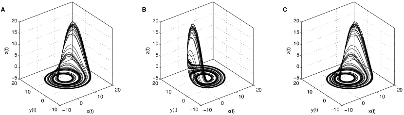
Figure 17: (A) Phase space trajectory of the Rössler system (Eqs. • ‣ A, with $a=0.15$, $b=0.2$ and $c=10$). (B) Same trajectory as in (A) but rotated on the $z$-axis by $\frac{3}{5}\pi$. (C) Same trajectory as in (A) but time scale transformed by $\tilde{t}=t^{2}$.

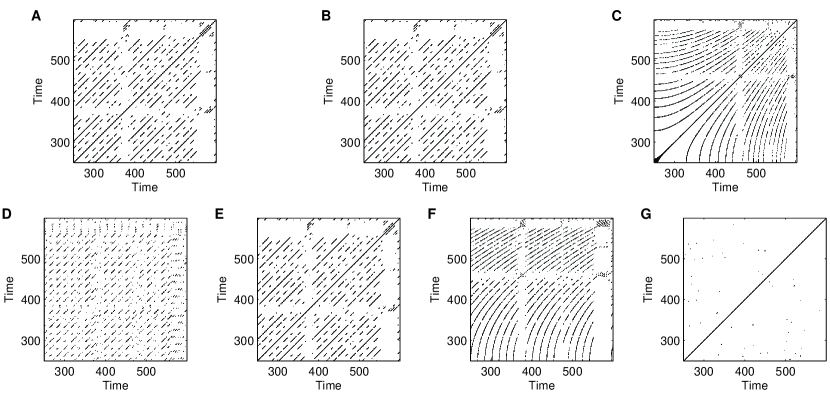
Figure 18: RPs of the (A) original trajectory of the Rössler system, (B) of the rotated trajectory and (C) of the stretched/compressed trajectory. (D) CRP and (E) JRP of the original and rotated trajectories and (F) CRP and (G) JRP of the original and stretched/compressed trajectories. The threshold for recurrence is $\varepsilon=1$.

Now we calculate the CRP between the original trajectory and the rotated one (Fig. 18D) and observe, that it is rather different from the RP of the original trajectory (Fig. 18A). This is because in the CRP the difference between each pair of vectors is computed, and this difference is not invariant under rotation of one of the systems. Hence, a rotation of the reference system of one trajectory changes the CRP. Therefore, the CRP cannot detect that both trajectories are identical up to a rotation. In contrast, the JRP of the original trajectory and the rotated one (Fig. 18E) is identical to the RP of the original trajectory (Fig. 18A). This is because the JRP considers joint recurrences, i. e. recurrences which occur simultaneously in both systems, and they are invariant under affine transformations.

The CRP between the original trajectory and the stretched/compressed one contains the bowed LOS, which reveals the functional shape of the parabolic transformation of the time scale (Fig. 18F). Note that the CRP represents the times at which both trajectories visit the same region of the phase space. On the other hand, the JRP of these trajectories is almost empty (Fig. 18G) because the recurrence structure of both systems is now different. Both trajectories have different time scales, and hence, there are almost no joint recurrences. Therefore, the JRP is not able to detect the time transformation applied to the trajectory, even though the shape of the phase space trajectories is very similar.

To conclude we can state that CRPs are more appropriate to investigate relationships between the parts of the same system which have been subjected to different physical or mechanical processes, e. g., two borehole cores in a lake subjected to different compression rates (see Subsec. 4.4). On the other hand, JRPs are more appropriate for the investigation of two interacting systems which influence each other, and hence, adapt to each other, e. g., in the framework of phase and generalised synchronisation (see Subsecs. 3.8, 4.7).

3.5 Measures of complexity (recurrence quantification analysis, RQA)

In order to go beyond the visual impression yielded by RPs, several measures of complexity which quantify the small-scale structures in RPs (Subsec. 3.2.2), have been proposed in [50, 101, 14] and are known as recurrence quantification analysis (RQA). These measures are based on the recurrence point density and the diagonal and vertical line structures of the RP. A computation of these measures in small windows (sub-matrices) of the RP moving along the LOI yields the time dependent behaviour of these variables. Some studies based on RQA measures show that they are able to identify bifurcation points, especially chaos-order transitions [102]. The vertical structures in the RP are related to intermittency and laminar states. Those measures quantifying the vertical structures enable also to detect chaos-chaos transitions [14].

In the following, we focus on the application of the RQA to RPs, but it is important to emphasise that the RQA can also be analogously applied to CRPs and JRPs. However, some of the interpretations of the RQA given below are not valid for CRPs. Henceforth, we assume that the RP is calculated by using a fixed threshold $\varepsilon$ (hence the RP is symmetric).

First, we introduce several such measures and then their potentials and limits for the identification of changes are discussed.

3.5.1 Measures based on the recurrence density

The simplest measure of the RQA is the recurrence rate ($RR$) or per cent recurrences

$$RR(\varepsilon)=\frac{1}{N^{2}}\sum_{i,j=1}^{N}\mathbf{R}_{i,j}(\varepsilon),$$ (41)

which is a measure of the density of recurrence points in the RP. Note that it corresponds to the definition of the correlation sum, Eq. (19), except that the LOI is usually not included. Furthermore, in the limit $N\to\infty$, $RR$ is the probability that a state recurs to its $\varepsilon$-neighbourhood in phase space. On the other hand, the $RR$ of CRPs corresponds to the cross correlation sum [73]

$$CC_{2}(\varepsilon)=\frac{1}{N^{2}}\sum_{i,j=1}^{N}\mathbf{CR}_{i,j}(\varepsilon),$$ (42)

and the $RR$ of JRPs of $n$ systems to the joint correlation sum

$$JC_{2}(\varepsilon^{(1)},\dots,\varepsilon^{(n)})=\frac{1}{N^{2}}\sum_{i,j=1}^{N}\prod_{k=1}^{n}\mathbf{R}^{\vec{x}_{(k)}}_{i,j}(\varepsilon^{(k)}).$$ (43)

The value

$$N_{\text{n}}(\varepsilon)=\frac{1}{N}\sum_{i,j=1}^{N}\mathbf{R}_{i,j}(\varepsilon)$$ (44)

is simply the average number of neighbours that each point on the trajectory has in its $\varepsilon$-neighbourhood.

3.5.2 Measures based on diagonal lines

The next measures are based on the histogram $P(\varepsilon,l)$ of diagonal lines of length $l$, i. e.

$$P(\varepsilon,l)=\sum_{i,j=1}^{N}\bigl{(}1-\mathbf{R}_{i-1,j-1}(\varepsilon)\bigr{)}\bigl{(}1-\mathbf{R}_{i+l,j+l}(\varepsilon)\bigr{)}\prod_{k=0}^{l-1}\mathbf{R}_{i+k,j+k}(\varepsilon).$$ (45)

In the following subsections we omit the symbol $\varepsilon$ from the RQA measures for the sake of simplicity (i. e. $P(l)=P(\varepsilon,l)$).

Processes with uncorrelated or weakly correlated, stochastic or chaotic behaviour cause none or very short diagonals, whereas deterministic processes cause longer diagonals and less single, isolated recurrence points. Therefore, the ratio of recurrence points that form diagonal structures (of at least length $l_{\min}$) to all recurrence points

$$DET=\frac{\sum_{l=l_{\min}}^{N}l\,P(l)}{\sum_{l=1}^{N}l\,P(l)}$$ (46)

is introduced as a measure for determinism (or predictability) of the system. The threshold $l_{\min}$ excludes the diagonal lines which are formed by the tangential motion of the phase space trajectory. For $l_{\min}=1$ the determinism is one. The choice of $l_{\min}$ could be made in a similar way as the choice of the size for the Theiler window [58], but we have to take into account that the histogram $P(l)$ can become sparse if $l_{\min}$ is too large, and, thus, the reliability of $DET$ decreases.

A diagonal line of length $l$ means that a segment of the trajectory is rather close during $l$ time steps to another segment of the trajectory at a different time; thus these lines are related to the divergence of the trajectory segments. The average diagonal line length

$$L=\frac{\sum_{l=l_{\min}}^{N}l\,P(l)}{\sum_{l=l_{\min}}^{N}P(l)}$$ (47)

is the average time that two segments of the trajectory are close to each other, and can be interpreted as the mean prediction time.

Another RQA measure considers the length $L_{\text{max}}$ of the longest diagonal line found in the RP, or its inverse, the divergence,

$$L_{\max}=\max\left(\left\{l_{i}\right\}_{i=1}^{N_{l}}\right)\quad\text{respectively}\quad DIV=\frac{1}{L_{\max}}.$$ (48)

where $N_{l}=\sum_{l\geq l_{\min}}P(l)$ is the the total number of diagonal lines. These measures are related to the exponential divergence of the phase space trajectory. The faster the trajectory segments diverge, the shorter are the diagonal lines and the higher is the measure $DIV$.

Eckmann et al. have stated that “the length of the diagonal lines is related to the largest positive Lyapunov exponent” if there is one in the considered system [2]. Different approaches have been suggested in order to use these lengths, Eqs. (47) and (48), to estimate the largest positive Lyapunov exponent, such as computing the $DIV$ [102] or the average of the inverse of the half lengths of the diagonals (using perpendicular RPs) [66]. However, the relationship between these measures and the positive Lyapunov exponent is not as simple as it was mostly stated in the literature. As already mentioned, the $K_{2}$ entropy is related with the (cumulative) frequency distribution of the lengths of the diagonal lines and, therefore, with the lower limit of the sum of the positive Lyapunov exponents. In Subsec. 3.6 we explain this relationship in detail and show how $L_{\max}$ can be used as an estimator for $K_{2}$ (and, hence, for the lower limit of the sum of the positive Lyapunov exponents).

The measure entropy refers to the Shannon entropy of the probability $p(l)=\frac{P(l)}{N_{l}}$ to find a diagonal line of exactly length $l$ in the RP,

$$ENTR=-\sum_{l=l_{\min}}^{N}p(l)\ln p(l).$$ (49)

$ENTR$ reflects the complexity of the RP in respect of the diagonal lines, e. g. for uncorrelated noise the value of $ENTR$ is rather small, indicating its low complexity.

The measures introduced up to now, $RR$, $DET$, $L$ etc. can also be computed separately for each diagonal parallel to the LOI. Henceforth, RQA measures for a certain line parallel to the LOI and with distance $\tau$ from the LOI are called $\tau$-recurrence rate, $\tau$-determinism etc., and the measures are marked with a subscribed index, like $RR_{\tau}$, $DET_{\tau}$, $L_{\tau}$ etc. Following this procedure, we need to define the number of diagonal lines $P_{\tau}(l)$ of length $l$ on each diagonal $\mathbf{RR}_{i,i+\tau}$ parallel to the LOI. $\tau=0$ corresponds to the main diagonal, $\tau>0$ to diagonals above and $\tau<0$ diagonals below the LOI (i. e. $\mathbf{RR}_{i+|\tau|,i}$), which represent positive and negative time delays, respectively.

The $\tau$-recurrence rate for those diagonal lines with distance $\tau$ from the LOI is then

$$RR_{\tau}=\frac{1}{N-\tau}\sum_{i=1}^{N-\tau}\mathbf{R}_{i,i+\tau}=\frac{1}{N-\tau}\sum_{l=1}^{N-\tau}l\,P_{\tau}(l).$$ (50)

This measure corresponds to the close returns histogram introduced for quantifying close returns plots [69]. It can be considered as a generalised auto-correlation function, as it also describes higher order correlations between the points of the trajectory in dependence on $\tau$. A further advantage with respect to the linear auto-correlation function is that $RR_{\tau}$ can be determined for a trajectory in phase space and not only for a single observable of the system’s trajectory. It can be interpreted as the probability that a state recurs to its $\varepsilon$-neighbourhood after $\tau$ time steps.

Analogous to the RQA, the $\tau$-determinism

$$DET_{\tau}=\frac{\sum_{l=l_{min}}^{N-\tau}l\,P_{\tau}(l)}{\sum_{l=1}^{N-\tau}l\,P_{\tau}(l)}$$ (51)

is the proportion of recurrence points forming diagonal lines longer than $l_{min}$ to all recurrence points, and the $\tau$-average diagonal line length

$$L_{\tau}=\frac{\sum_{l=l_{min}}^{N-\tau}l\,P_{\tau}(l)}{\sum_{l=l_{min}}^{N-\tau}P_{\tau}(l)}$$ (52)

is the mean length of the diagonal structures on the considered diagonal parallel to the LOI. The $\tau$-entropy can be applied to the diagonal-wise consideration as well.

These diagonal-wise computed measures, $RR_{\tau}$, $DET_{\tau}$ and $L_{\tau}$, over time distance $\tau$ from the LOI can be used, e. g., to determine the Theiler window. This diagonal-wise determination of the RQA measures plays an important role in the analysis of CRPs as well. Long diagonal structures in the CRP reveal a similar time evolution of the trajectories of both processes. It is obvious that a progressively increased similarity between both processes causes an increase of the recurrence point density along the main diagonal $\mathbf{CR}_{i,i}\,|_{i=1}^{N}$ until finally the LOI appears and the CRP becomes an RP. Thus, the occurrence of diagonal lines in a CRP can be used in order to benchmark the similarity between the considered processes. Using this approach it is possible to assess the similarity in the dynamics of two different systems in dependence on a certain time delay.

The $\tau$-recurrence $RR_{\tau}$ of a CRP reveals the probability of the occurrence of similar states in both systems with a certain delay $\tau$. $RR_{\tau}$ has a high value for systems whose trajectories often visit the same phase space regions.

As already mentioned, stochastic as well as strongly fluctuating processes cause none or only short diagonals, whereas deterministic processes cause longer diagonals. If two deterministic processes have the same or similar time evolution, i. e. parts of the phase space trajectories visit the same phase space regions for certain times, the amount of longer diagonals increases and the amount of shorter diagonals decreases. The $\tau$-determinism $DET_{\tau}$ of a CRP is related to the similar time evolution of the systems’ states. The measure $L_{\tau}$ quantifies the duration of the similarity in the dynamics of both systems. A high coincidence of both trajectories increases the length of these diagonals.

Considering CRPs, smooth trajectories with long auto-correlation times will result in a CRP with long diagonal structures, even if the trajectories are not linked to each other (this effect corresponds to the tangential motion of one trajectory). In order to avoid counting such “false” diagonals, the lower limit for the diagonal line length $l_{min}$ should be of the order of the auto-correlation time.

By applying a measure of symmetry and asymmetry on the $\tau$-RQA measures (for a small range $0\leq\tau\ll N$), e. g. on $RR_{\tau}$,

$$Q(\tau)=\frac{RR_{\tau}+RR_{-\tau}}{2},\quad\text{and}\quad q(\tau)=\frac{RR_{\tau}-RR_{-\tau}}{2},$$ (53)

we can simply quantify interrelations between two systems and are able to determine which system leads the other (Fig. 19; this is similar to an approach for the detection of event synchronisation proposed in [103]).

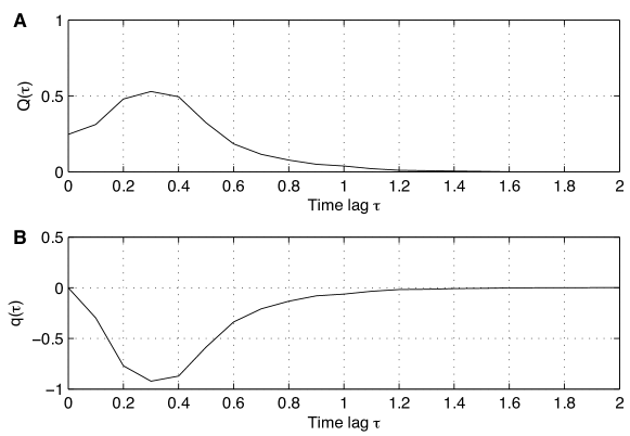
Figure 19: Measure of symmetry (A) and asymmetry (B) applied on the diagonal-wise computed recurrence rate $RR_{\tau}$ of the CRP of two mutually coupled Rössler systems in the funnel regime, Eqs. (• ‣ A) and (• ‣ A), for $a=0.2925$, $b=0.1$, $c=8.5$, $\nu=0.02$, with a slight time lag. (A) The maxima for the symmetry measure $Q(\tau)$ at a time lag of $k=0.3$ reveals the synchronisation between both systems after the detected lag. (B) The negative value of the asymmetry measure $q(\tau)$ at this lag reveals that the second Rössler oscillator leads the first one.

Summarising, we can state that high values of $RR_{\tau}$ indicate a high probability of occurrence of the same state in both systems, and high values of $DET_{\tau}$ and $L_{\tau}$ indicate a long time span, in which both systems visit the same region of phase space. Therefore, $DET_{\tau}$ and $L_{\tau}$ are sensitive to fast and strongly fluctuating data. It is important to emphasise that these parameters are statistical measures and that their validity increases with the size of the CRP, i. e. with the length of the regarded trajectory.

The consideration of an additional CRP

$$\mathbf{CR}^{-}_{i,j}=\Theta\left(\varepsilon-\left\|\vec{x}_{i}+\vec{y}_{j}\right\|\right)$$ (54)

with a negative signed second trajectory $-\vec{y}_{j}$ allows distinguishing correlation and anti-correlation between the considered trajectories [96]. In order to recognise the measures for both possible CRPs, the superscript index $+$ is added to the measures for the positive linkage and the superscript index $-$ for the negative linkage, e. g. $RR^{+}_{\tau}$ and $RR^{-}_{\tau}$.

Another approach used to study positive and negative relations between the considered trajectories involves the composite measures for the $\tau$-recurrence rate

$$RR^{c}_{\tau}=\frac{1}{N-k}\sum_{j-i=k}\left(\mathbf{CR}^{+}_{i,j}-\mathbf{CR}^{-}_{i,j}\right),$$ (55)

the $\tau$-determinism

$$DET^{c}_{\tau}=DET^{+}_{\tau}-DET^{-}_{\tau},$$ (56)

and the $\tau$-average diagonal length

$$L^{c}_{\tau}=L^{+}_{\tau}-L^{-}_{\tau},$$ (57)

as it was used in [7]. This presentation is similar to the time-dependent presentation of the cross correlation function (but with the important difference that the $\tau$-RQA measures consider also higher order moments) and is more intuitive than the separate representation of $RR_{\tau}^{+}$, $RR_{\tau}^{-}$ etc. However, for the investigation of interrelations based on even functions, these composite measures are not suitable.

A further substantial advantage of applying the $\tau$-RQA on CRPs is the capability to find also nonlinear similarities in short and non-stationary time series with high noise levels as they typically occur, e. g., in life or earth sciences. In these cases, using a fixed amount of nearest neighbours is more appropriate than a fixed threshold $\varepsilon$. Also the use of OPRPs or JRPs is appropriate for the analysis of this kind of data.

Note that the $\tau$-RQA measures as functions of the distance $\tau$ to the main diagonal are also important for the quantification of RPs. For example, the measure $RR_{\tau}$ can be used to find UPOs in low-dimensional chaotic systems [104, 69, 48]. Since periodic orbits are more closely related to the occurrence of longer diagonal structures, the measures $DET_{\tau}$ and $L_{\tau}$ are more suitable candidates for this kind of study. The measure $RR_{\tau}$ has been already used in [2] for the study of non-stationarity in the data. Beyond this, $RR_{\tau}$ can be applied to analyse synchronisation between oscillators (Subsec. 3.8).

Another RQA measure is the trend, which is a linear regression coefficient over the recurrence point density $RR_{\tau}$ of the diagonals parallel to the LOI as a function of the time distance between these diagonals and the LOI

$$TREND=\frac{\sum_{\tau=1}^{\tilde{N}}(\tau-\tilde{N}/2)(RR_{\tau}-\langle RR_{\tau}\rangle)}{\sum_{\tau=1}^{\tilde{N}}(\tau-\tilde{N}/2)^{2}}.$$ (58)

It provides information about non-stationarity in the process, especially if a drift is present in the analysed trajectory. The computation excludes the edges of the RP ($\tilde{N}<N$) because of the lack of a sufficient number of recurrence points. The choice of $\tilde{N}$ depends on the studied system. Whereas $N-\tilde{N}>10$ should be sufficient for noise, this difference should be much larger for a system with some auto-correlation length (ten times the order of magnitude of the auto-correlation time should be enough). It should be noted that if the time dependent RQA (measures computed in sliding windows) is used, $TREND$ will depend strongly on the size of the window and may yield ambiguous results for different window sizes.

A further measure, the ratio, has been defined as the ratio between $DET$ and $RR$ [101]. It can be computed based on the number $P(l)$ of diagonal lines of length $l$ as follows

$$RATIO=N^{2}\,\frac{\sum_{l=l_{min}}^{N}l\,P(l)}{\left(\sum_{l=1}^{N}l\,P(l)\right)^{2}}.$$ (59)

A heuristic study of physiological time series has revealed that this ratio can be used to uncover transitions in the dynamics; during certain types of qualitative transitions $RR$ decreased, whereas $DET$ remained constant [101].

The RQA measures discussed so far, are based on diagonal structures in the RP. In Subsec. 3.5.3, this quantitative view is extended to vertical (horizontal) structures and further measures of complexity based on the distribution of the vertical lines are proposed.

Example: Finding nonlinear interrelations by applying RQA on CRPs

This example shows the ability of CRPs to find nonlinear interrelations between two processes, which cannot be detected by means of linear tests [96]. We consider linear correlated noise (auto-regressive process) which is nonlinearly coupled with the $x$-component of the Lorenz system (for standard parameters $\sigma=10$, $r=28$, $b=8/3$ and a time resolution of $\Delta t=0.01$ [78, 105]):

$$y_{i}=0.86\,y_{i-1}+0.500\,\xi_{i}+\kappa\,x_{i}^{2},$$ (60)

where $\xi$ is Gaussian white noise and $x_{i}$ ($x(t)\rightarrow x_{i}$, $t=i\,\Delta t$) is normalised with respect to the standard deviation. The data length is 8,000 points and the coupling $\kappa$ is realised without any lag.

As expected, due to the nonlinear linkage the cross correlation analysis between $x$ and $y$ does not reveal a significant linear correlation between these data series (Fig. 20A). However, the mutual information as a well-established measure to detect nonlinear dependencies [46] shows a strong dependence between $x$ and $y$ at a delay of $0.05$ (Fig. 20B). The CRP based $\tau$-recurrence rate $RR_{\tau}$ and $\tau$-average diagonal length $L_{\tau}$ exhibit maxima at a lag of about $0.05$ for $RR^{+}$/$L^{+}$ and $RR^{-}_{\tau}$/$L^{-}_{\tau}$ and additionally at $0.45$ and $-0.32$ for $RR^{-}_{\tau}$/$L^{-}_{\tau}$ (Fig. 20C, D). The maxima around $0.05$ for the $+$ and $-$ measures are a strong indication of a nonlinear relationship between the data. The delay of approximately $0.05$ stems from the auto-correlation of $y$ and approximately corresponds to its correlation time $\Delta t/\ln{0.86}=0.066$. The maxima at $0.45$ and $-0.32$ correspond to the half mean period of the Lorenz system. Since the result is rather independent of the sign of the second data, the found interrelation is of the kind of an even function. 500 realisations of the AR model have been used in order to estimate the distributions of the measures. The $2\sigma$ margins of these distributions can be used to assess the significance of the results.

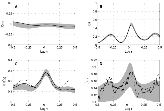
Figure 20: (A) Cross correlation $C(\tau)$, (B) mutual information $I(\tau)$, (C) $\tau$-recurrence rate $RR_{\tau}$ and (D) $\tau$-average line length $L_{\tau}$ for the forced auto-regressive process and the forcing function; the curves represent the measures for one realisation as functions of the delay $\tau$ for a coupling $\kappa=0.2$. In (C) and (D) the solid lines show positive relation; the dashed lines show negative relation. The grey bands mark the $2\sigma$ margin of the distributions of the measures gained from 500 realisations. The lag $\tau$ and the average line length $L_{\tau}$ have units of time [96].

Due to the rapid fluctuation of $y$, the number of long diagonal lines in the CRP decreases. Therefore, measures based on these diagonal structures, especially $DET_{\tau}$, do not work well with such heavily fluctuating data. However, we can infer that the measures $RR_{\tau}$ as well as $L_{\tau}$ (though less significant for rapidly fluctuating data) are suitable for finding a nonlinear relation between the considered data series $x$ and $y$, where the linear analysis is not able to detect such a relation. Furthermore, this technique is applicable to rather short and non-stationary data compared to the mutual information.

3.5.3 Measures based on vertical lines

A vertical line of length $v$ starting at the coordinates $(i,j)$ of a RP is given by the condition (16). In continuous time systems discretised with sufficiently high time resolution and with an appropriate large threshold $\varepsilon$, a large part of these vertical lines usually correspond to the tangential motion of the phase space trajectory (Fig. 21). However, not all elements of these sets belong to the tangential motion. For example, even though there is no tangential motion in maps, we find vertical lines in their RPs, e. g. in the presence of laminar states in intermittent regimes. Furthermore, in systems with two different time scales, we might find vertical lines because of the finite size of the threshold $\varepsilon$, and not because of tangential motion. Sometimes, the points belonging to the tangential motion are called sojourn points [34]. But we will not use this term, because it is a bit misleading, and actually those points forming vertical lines but which do not belong to the tangential motion would be the sojourn points.

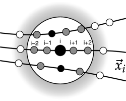
Figure 21: States of subsequent time may fall into the neighbourhood of the state at time $i$, pretending artificial recurrences (grey dots). This is called tangential motion and such points are referred to as sojourn points.

The total number of vertical lines of the length $v$ in the RP is then given by the histogram

$$P(v)=\sum_{i,j=1}^{N}\bigl{(}1-\mathbf{R}_{i,j}\bigr{)}\bigl{(}1-\mathbf{R}_{i,j+v}\bigr{)}\prod_{k=0}^{v-1}\mathbf{R}_{i,j+k}.$$ (61)

Analogous to the definition of the determinism, Eq. (46), the ratio between the recurrence points forming the vertical structures and the entire set of recurrence points can be computed,

$$LAM=\frac{\sum_{v=v_{min}}^{N}vP(v)}{\sum_{v=1}^{N}vP(v)},$$ (62)

and is called laminarity. The computation of $LAM$ is realised for those $v$ that exceed a minimal length $v_{min}$ in order to decrease the influence of the tangential motion. For maps, $v_{min}=2$ is an appropriate value. $LAM$ represents the occurrence of laminar states in the system without describing the length of these laminar phases. $LAM$ will decrease if the RP consists of more single recurrence points than vertical structures.

The average length of vertical structures is given by (cf. Eq. (47))

$$TT=\frac{\sum_{v=v_{min}}^{N}vP(v)}{\sum_{v=v_{min}}^{N}P(v)},$$ (63)

and is called trapping time. Its computation requires also the consideration of a minimal length $v_{min}$, as in the case of $LAM$. $TT$ estimates the mean time that the system will abide at a specific state or how long the state will be trapped.

Finally, the maximal length of the vertical lines in the RP

$$V_{\max}=\max\left(\left\{v_{l}\right\}_{l=1}^{N_{v}}\right)$$ (64)

can be regarded, analogously to the standard measure $L_{\max}$ ($N_{v}$ is the absolute number of vertical lines).

In contrast to the RQA measures based on diagonal lines, these measures are able to find chaos-chaos transitions [14]. Hence, they allow for the investigation of intermittency, even for rather short and non-stationary data series. Furthermore, since for periodic dynamics the measures quantifying vertical structures are zero, chaos-order transitions can also be identified.

Example: Comparison of measures based on diagonal and vertical lines

Next, we illustrate the application of the RQA for the logistic map, Eq. (127), and compare the measures based on diagonal with the ones based one vertical structures. We generate for each value of the control parameter $a\in[3.5,4]$, with $\Delta a=0.0005$ a separate time series (Fig. 22) of the rather short length $1,000$. In the analysed range of $a$, various dynamical regimes and transitions between them occur, e. g., accumulation points, periodic and chaotic states, band merging points, period doublings, inner and outer crises, i. e. system (127) generates various order-chaos, chaos-order as well as chaos-chaos transitions. [106].

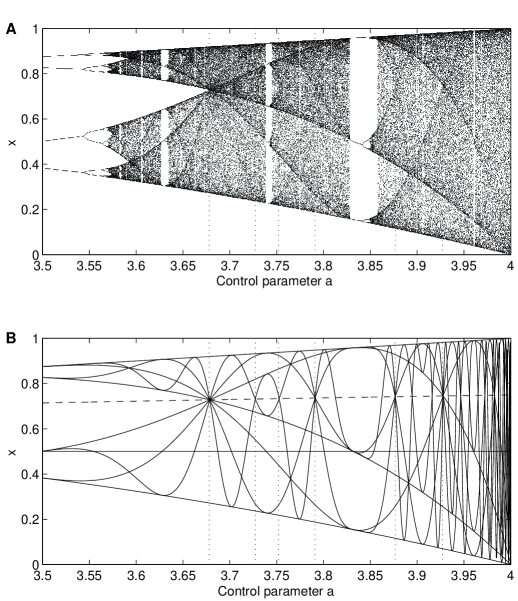
Figure 22: (A) Bifurcation diagram of the logistic map. (B) Low ordered supertrack functions $s_{i}(a)\,|_{i=1}^{10}$ and the fixed point of the logistic map $1-1/a$ (dashed). Their intersections represent periodic windows, band merging and laminar states. The dotted lines show a choice of points, which represent band merging and laminar phases ($a=3.678$, $3.727$, $3.752$, $3.791$, $3.877$, $3.927$) [14].

Useful tools for studying the chaotic behaviour of the logistic map are the supertrack functions, which are recursively generated from

$$s_{i+1}(a)=a\,s_{i}(a)\bigl{(}1-s_{i}(a)\bigr{)},\quad s_{0}(a)=\frac{1}{2},\quad i=1,\,2,\,\ldots$$ (65)

$s_{i}(a)$ represent the functional dependence of stable states at a given iteration number $i$ on the control parameter $a$ [107]. The intersection of $s_{i}(a)$ with $s_{i+j}(a)$ indicates the occurrence of a $j$-period cycle, and the intersection of $s_{i}(a)$ with the fixed-point $(1-1/a)$ of the logistic map indicates the point of an unstable singularity, i. e. laminar behaviour (Fig. 22, intersection points are marked with dotted lines).

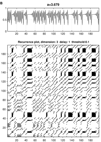
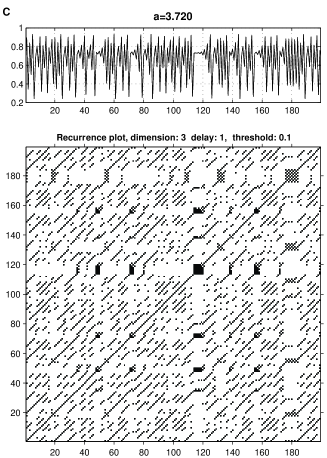
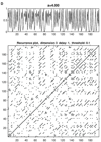
Figure 23: RPs of the logistic map for various values of the control parameters $a$: (A) periodic-3-window $a=3.830$, (B) band merging $a=3.679$, (C) supertrack intersection $a=3.720$ and (D) chaos (exterior crisis) $a=4$; with embedding dimension $m=3$, time delay $\tau=1$ and threshold $\varepsilon=0.1\sigma$ [14].

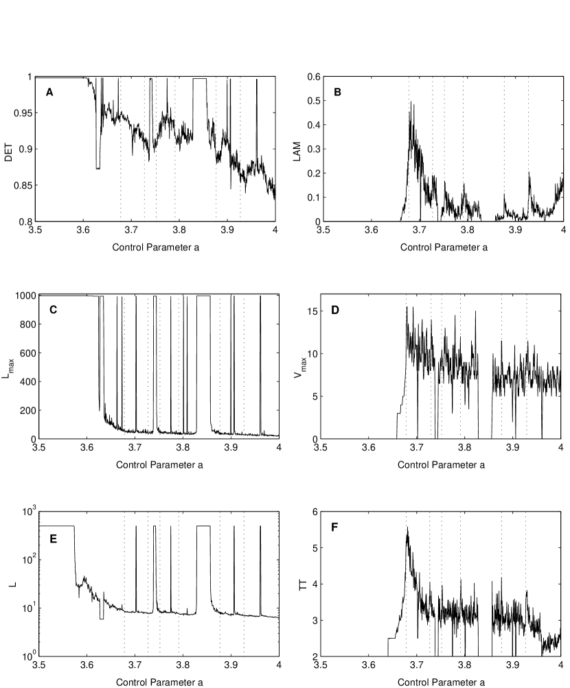
Figure 24: Selected RQA measures $DET$, $L_{\max}$ and $L$ and the measures $LAM$, $V_{\max}$ and $TT$. The vertical dotted lines indicate some of the points, at which band merging and laminar behaviour occur (cf. Fig. 22), whereby not all of them have been marked. Whereas (A) $DET$, (C) $L_{\max}$ and (E) $L$ show periodic-chaos/chaos-periodic transitions (maxima), (B) $LAM$, (D) $V_{\max}$ and (F) $TT$ exhibit in addition to those transitions (minima) chaos-chaos transitions (maxima). The differences between $LAM$ and $V_{\max}$ are caused by the fact that $LAM$ measures only the amount of laminar states, whereas $V_{\max}$ measures the maximal duration of the laminar states. Although some peaks of $V_{\max}$ and $TT$ are not at the dotted lines, they correspond to laminar states (not all can be marked) [14].

Although an embedding is not necessary for maps (i. e. $m=1$), we use here an embedding of $m=3$ and $\tau=1$ in order to compare the results with [102]. The cut-off distance $\varepsilon$ is selected to be 10% of the standard deviation of the data series. Smaller values would lead to a better distinction of small variations (e. g. the range before the accumulation point consists of small variations), but the recurrence point density would decrease and hence, the statistics of continuous structures in the RP would become poor.

RPs for various values of the control parameter $a$ exhibit already visually specific characteristics (Fig. 23). Periodic states cause continuous and periodic diagonal lines in the RP, but no vertical or horizontal lines (Fig. 23A). On the other hand, chaos-chaos transitions, as band merging points, inner crises or regions of intermittency represent states with short laminar behaviour and cause vertically and horizontally spread black areas in the RP (Fig. 23B, C). Moreover, diagonal lines occur. The fully developed chaotic state ($a=4$) causes a rather homogeneous RP with numerous single points and some short (in comparison to the length of the LOI), diagonal or vertical lines (Fig. 23D). Vertical (and horizontal) lines occur much more frequently at supertrack crossing points (chaos-chaos transitions) than in other chaotic regimes (Fig. 22).

The measures $DET$, $L$ and $L_{\max}$, which are basing on the diagonal lines, show clear maxima at the periodic-chaos/chaos-periodic transitions. The measure $L_{\max}$ finds all of such transitions, but $DET$ and $L$ do not detect all of them (Fig. 24A, C, E and Tab. 2). However, they all are not able to detect chaos-chaos transitions. But, the chaos-chaos transitions to the laminar states are identified by the measures $LAM$, $TT$ and $V_{\max}$, which are based on the vertical structures (Fig. 24B, D, F and Tab. 2). These measures show distinct maxima or peaks at the chaos-chaos transitions. Furthermore, the measures fall to zero within the period windows, hence, the chaos-order transitions can also be identified. Since vertical lines occur much more frequently at inner crisis, band merging points and in regions of intermittency (i. e. laminar states) than in other chaotic regimes, $TT$ and $V_{\max}$ grow up significantly at those points. This can also be seen by looking at the supertrack functions (Fig. 22B). Although $LAM$ also reveals laminar states, it is quite different from the other two measures because it does not increase at inner crises (Tab. 2). Noise, of course, influences these results. For small noise levels, the transitions can still be identified. Moreover, $LAM$ is more robust against noise than $TT$ and $V_{\max}$ [14].

The behaviour of these measures regarding the control parameter $a$ is similar to some of formerly proposed measures of complexity [108, 109]. The Rényi dimension $D_{q}$ of order $q<0$, the fluctuation complexity as well as the re-normalised entropy exhibit local maxima in regions of intermittency, a rapid increase at inner crises and a rapid decrease and increase at the transitions between chaos and periodic windows. The difference between the formerly proposed measures and $LAM$, $TT$ and $V_{\max}$ is the amount of data points needed. It is important to emphasise that for the methods proposed in [108] and [109], more than 100,000 data points are needed, whereas 1,000 data points are enough for the measures based on RPs.

Table 2: Comparison of RQA measures based on diagonal ($DET$, $L$ and $L_{\max}$) and vertical structures ($LAM$, $TT$ and $V_{\max}$) regarding periodic-chaos/chaos-periodic transitions (PC/CP), chaos-chaos transitions (band merging – BM and inner crisis – IC) and laminar states.

measure	PC/CP transitions	BM and IC	laminar states
$DET$	increases	–	–
$L$	increases	–	–
$L_{\max}$	increases	–	–
$LAM$	drops to zero	–	increases
$TT$	drops to zero	increases	increases
$V_{\max}$	drops to zero	increases	increases

3.6 Dynamical invariants derived from RPs

The RQA measures introduced in Subsec. 3.5 are rather heuristic but describe RPs quantitatively and are especially helpful to find various transitions in dynamical systems. However, their major drawback is that they are typically not invariant with respect to the embedding used to reconstruct the phase space trajectory, i. e. the values of the RQA measures depend rather strongly on the embedding parameters. Therefore, it is important to know, whether typical invariants in nonlinear dynamics, like entropies or dimensions, can be inferred from the recurrence matrix, too.

Let us start with the generalised correlation sum (the generalisation of Eq. (19)),

$$C_{q}(\varepsilon)=\left\{\frac{1}{N}\sum_{i=1}^{N}\left[\frac{1}{N}\sum_{j=1}^{N}\Theta\left(\varepsilon-\|\vec{x}_{i}-\vec{x}_{j}\|\right)\right]^{q-1}\right\}^{\frac{1}{q-1}},$$ (66)

which can be used to estimate generalised entropies, dimensions, mutual information and redundancies (e. g. [110, 111, 112, 59, 113]). From Eq. (66) it is obvious that the density of recurrence points in an RP can also be used to estimate these invariants. However, some of these invariants, such as the mutual information and the generalised entropies, are related to further features of RPs and not just the density of recurrence points.

As we have mentioned in Subsec. 3.5, an important ingredient for the computation of the RQA measures is the length-distribution of diagonal lines $P(\varepsilon,l)$ in the RP, Eq. (45), because it encodes main properties of the system, such as predictability and measures of complexity. Diagonal lines in the RP represent co-moving segments of different parts of the trajectory $\vec{x}_{i+k}$ and $\vec{x}_{j+k}$ for some $k=1,\ldots,l$, Eqs. (13) and (14). The longer the trajectories move within an $\varepsilon$-tube (cf. Fig. 2), the longer the diagonal lines in the RP will be. As the time for which trajectories starting at close initial conditions move within an $\varepsilon$-tube is related to the inverse of the largest Lyapunov exponent, it can be supposed that also the length of the diagonal lines in an RP can be linked to the predictability of the underlying system. Since the introduction of RPs a relationship between the length of the diagonal lines and the maximal Lyapunov exponent has been stated [2]. As already mentioned, several attempts have been tried to heuristically fix this relationship as a direct inverse relation between the maximal or averaged line length and the Lyapunov exponent [102, 68]. Choi et al. introduced a measure based on the width and the absolute number of diagonal lines and related this measure to the largest Lyapunov exponent [66]. However, we show next that the distribution of diagonal lines is not directly related to the maximal Lyapunov exponent but to the correlation entropy [114, 115, 116, 8]. The formal relationship between the correlation entropy and the Lyapunov exponents [117, 118] is

$$K_{2}\leq\sum_{\lambda_{i}>0}\lambda_{i},$$ (67)

where $\lambda_{i}$ denote the Lyapunov exponents. Moreover, the algorithm for the estimation of these invariants gives some justification for the ad hoc measures of the RQA.

3.6.1 Correlation entropy and correlation dimension

At first, the definition of the Rényi entropy of second order is recalled in order to deduce how it is linked to the distribution of diagonal lines in the RP. Let us consider a trajectory $\vec{x}(t)$ in the basin of an attractor in a $d$-dimensional phase space. We divide the phase space into $d$-dimensional hyper-cubes of size $\varepsilon$. Then $p_{i_{1},\ldots,i_{l}}(\varepsilon)$ denotes the joint probability that $\vec{x}(t=1\,\Delta t)$ is in the $\varepsilon$-box $i_{1}$, $\vec{x}(t=2\,\Delta t)$ is in the box $i_{2}$, …, and $\vec{x}(t=l\,\Delta t)$ is in the box $i_{l}$. The second order Rényi entropy (correlation entropy) [111, 119] is then defined by

$$K_{2}=-\lim_{\Delta t\to 0}\lim_{\varepsilon\to 0}\lim_{l\to\infty}\frac{1}{l\Delta t}\ln\sum_{i_{1},\ldots,i_{l}}p^{2}_{i_{1},\dots,i_{l}}(\varepsilon).$$ (68)

Assuming that the system is ergodic, which is always the case for chaotic systems as they are mixing, we obtain

$$\sum_{i_{1},\ldots,i_{l}}p^{2}_{i_{1},\ldots,i_{l}}(\varepsilon)=\frac{1}{N}\sum_{t=1}^{N}p_{i_{1}(t),\ldots,i_{l}(t+(l-1)\Delta t)}(\varepsilon),$$ (69)

where $i_{1}(t)$ is the box that the $t^{th}$ data point is in, $i_{2}(t+\Delta t)$ is the box that the $(t+\Delta t)^{th}$ data point is in, etc. [113]. Furthermore, approximating $p_{i_{1}(t),\ldots,i_{l}(t+(l-1)\Delta)}(\varepsilon)$ by the probability $p_{t}(\varepsilon,l)$ of finding a sequence of $l$ points in boxes of size $\varepsilon$ centred at the points $\vec{x}(t),\dots,\vec{x}(t+(l-1)\Delta t)$, we can state

$$\frac{1}{N}\sum_{t=1}^{N}p_{i_{1}(t),\ldots,i_{l}(t+(l-1)\Delta t)}(\varepsilon)\approx\frac{1}{N}\sum_{t=1}^{N}p_{t}(\varepsilon,l).$$ (70)

Moreover, $p_{t}(\varepsilon,l)$ can be expressed by means of the recurrence matrix

$$p_{t}(\varepsilon,l)=\lim_{N\to\infty}\frac{1}{N}\sum_{s=1}^{N}\prod_{k=0}^{l-1}\mathbf{R}_{t+k,s+k}(\varepsilon).$$ (71)

Based on Eqs. (68)–(71), an estimator for the second order Rényi entropy can be found by means of the RP

$$\hat{K_{2}}(\varepsilon,l)=-\frac{1}{l\,\Delta t}\ln\left(p_{c}(\varepsilon,l)\right)=-\frac{1}{l\,\Delta t}\ln\left(\frac{1}{N^{2}}\sum_{t,s=1}^{N}\prod_{k=0}^{l-1}\mathbf{R}_{t+k,s+k}(\varepsilon)\right),$$ (72)

where $p_{c}(\varepsilon,l)$ is the probability to find a diagonal of at least length $l$ in the RP. Therefore, if we plot $p_{c}(\varepsilon,l)$ in a logarithmic scale versus $l$, we should obtain a straight line with slope $-\hat{K}_{2}(\varepsilon)\Delta t$ for large $l$.

On the other hand, the $l$-dimensional 2${}^{\text{nd}}$-order correlation sum

$$C_{2}(\varepsilon,l)=\lim_{N\to\infty}\frac{1}{N^{2}}\sum_{i,j=1}^{N}\Theta\left(\varepsilon-\sqrt{\sum_{k=0}^{l-1}\left\|\vec{x}_{i+k}-\vec{x}_{j+k}\right\|^{2}}\right).$$ (73)

can be used in the definition for $K_{2}$ [110]

$$K_{2}(\varepsilon,l)=-\lim_{\Delta t\to 0}\lim_{\varepsilon\to 0}\lim_{l\to\infty}\frac{1}{l\Delta t}\ln C_{2}(\varepsilon,l).$$ (74)

Due to the exponential divergence of the trajectories, the condition in Eq. (73)

$$\sum_{k=0}^{l-1}\left|\left|\vec{x}_{i+k}-\vec{x}_{j+k}\right|\right|^{2}\leq\varepsilon^{2}$$

is essentially equivalent to

$$\left|\left|\vec{x}_{i+k}-\vec{x}_{j+k}\right|\right|<\varepsilon\quad\text{for}\quad k=1,\ldots,l,$$

and, therefore, equivalent to the product in Eq. (71).

If only a scalar time series is available, embedding is used, Eq. (9). Taking the embedding dimension $l$ (here $l$ is used for the embedding dimension instead of $m$ for didactical reasons) and time delay $\tau=1$, the $l$-dimensional correlation sum can be estimated by

$$\tilde{C}_{2}(\varepsilon,l)=\lim_{N\to\infty}\frac{1}{N^{2}}\sum_{i,j=1}^{N}\Theta\left(\varepsilon-\sqrt{\sum_{k=0}^{l-1}\left|x_{i+k}-x_{j+k}\right|^{2}}\right).$$ (75)

Then, an estimator of $K_{2}$ (Grassberger-Procaccia (G-P) algorithm) can be obtained by

$$\tilde{K}_{2}(\varepsilon,l)=\frac{1}{\Delta t}\ln\frac{\tilde{C}_{2}(\varepsilon,l)}{\tilde{C}_{2}(\varepsilon,l+1)}.$$ (76)

Moreover, $C_{2}(\varepsilon,l)$ scales like $C_{2}(\varepsilon,l)\sim\varepsilon^{D_{2}}$ [120], what leads with Eq. (74) to

$$C_{2}(\varepsilon,l)\sim\varepsilon^{D_{2}}\e^{-l\,\Delta t\,K_{2}}.$$ (77)

Due to the similarity between the approaches using RPs and the correlation sum, we state the basic relation

$$p_{c}(\varepsilon,l)\approx\sum_{i_{1},\ldots,i_{l}}p^{2}(i_{1},\ldots,i_{l})\approx\tilde{C}_{2}(\varepsilon,l)\sim\varepsilon^{D_{2}}\e^{-l\,\Delta t\,K_{2}}.$$ (78)

The difference between both approaches is that in $p_{c}(\varepsilon,l)$ we include information about $l$ vectors, whereas in $\tilde{C}_{2}(\varepsilon,l)$ we have just information about $l$ coordinates. Besides this, in the RP approach $l$ is a length in the plot, whereas in the G-P algorithm $l$ means the embedding dimension.

The relationship (78) also allows to estimate $D_{2}$ from $p_{c}(\varepsilon,l)$. Considering Eq. (78) for two different thresholds $\varepsilon$ and $\varepsilon+\Delta\varepsilon$ and dividing both of them, we get

$$\hat{D}_{2}(\varepsilon)=\ln\left(\frac{p_{c}(\varepsilon,l)}{p_{c}(\varepsilon+\Delta\varepsilon,l)}\right)/\ln\left(\frac{\varepsilon}{\varepsilon+\Delta\varepsilon}\right),$$ (79)

which is an estimator of the correlation dimension $D_{2}$ [111].

Analogously to Eq. (72), the joint Rényi entropy of second order can be estimated using the probability to find a diagonal of at least length $l$ in the JRP instead of the RP of a single system. This extension of the estimator of Eq. (72) is useful for the analysis of two or more interacting systems, as will be shown in Subsec. 3.8. The joint Rényi entropy of second order is defined as

$$JK_{2}=-\lim_{\Delta t\to 0}\lim_{\varepsilon\to 0}\lim_{l\to\infty}\frac{1}{l\Delta t}\ln\sum_{\begin{subarray}{c}i_{1},\ldots,i_{l}\\ j_{1},\ldots,j_{l}\end{subarray}}p^{2}_{i_{1},\ldots,i_{l},j_{1},\ldots,j_{l}}(\varepsilon),$$ (80)

where $p_{i_{1},i_{2},\ldots,i_{l},j_{1},j_{2},\ldots,j_{l}}(\varepsilon)$ is the joint probability that $\vec{x}(t=\Delta t)$ is in box $i_{1}$, $\vec{x}(t=2\Delta t)$ is in box $i_{2}$, …, $\vec{x}(t=l\Delta t)$ is in box $i_{l}$ and simultaneously $\vec{y}(t=\Delta t)$ is in box $j_{1}$, $\vec{y}(t=2\Delta t)$ is in box $j_{2}$, …, and $\vec{y}(t=l\Delta t)$ is in box $j_{l}$. Using again the ergodicity of the system,

$$\sum_{\begin{subarray}{c}i_{1},\ldots,i_{l}\\ j_{1},\ldots,j_{l}\end{subarray}}p^{2}_{i_{1}(t),\ldots,i_{l}(t+(l-1)\Delta t),j_{1}(t),\ldots,j_{l}(t+(l-1)\Delta t)}=\frac{1}{N}\sum_{t=1}^{N}p_{i_{1},\ldots,i_{l},j_{1},\ldots,j_{l}}$$ (81)

can be stated. On the other hand, the following approximation

$$p_{i_{1}(t),\ldots,i_{l}(t+(l-1)\Delta t),j_{1}(t),\ldots,j_{l}(t+(l-1)\Delta t)}\approx{}$$

$${}\frac{1}{N}\sum_{s=1}^{N}\prod_{m=0}^{l-1}\Theta(\varepsilon^{\vec{x}}-\|\vec{x}_{t+m}-\vec{x}_{s+m}\|)\Theta(\varepsilon^{\vec{y}}-\|\vec{y}_{t+m}-\vec{y}_{s+m}\|)$$

can be made (cf. Eqs. (69) and (71)). Then, substituting this expression in Eq. (80), the estimator for the joint Rényi entropy of second order is

$$\widehat{JK_{2}}(\varepsilon^{\vec{x}},\varepsilon^{\vec{y}},l)=-\frac{1}{l\Delta t}\ln\underbrace{\left(\frac{1}{N^{2}}\sum_{t,s=1}^{N}\prod_{k=0}^{l-1}\mathbf{JR}_{t+k,s+k}(\varepsilon^{\vec{x}},\varepsilon^{\vec{y}})\right)}_{\ast}.$$ (83)

Note, that $\ast$ is the probability $p_{c}(\varepsilon^{\vec{x}},\varepsilon^{\vec{y}},l)$ to find a diagonal of at least length $l$ in the JRP. Hence, the logarithmic representation of $p_{c}(\varepsilon^{\vec{x}},\varepsilon^{\vec{y}},l)$ versus $l$ reveals a straight line for small thresholds $\varepsilon^{\vec{x}},\varepsilon^{\vec{y}}$ and long lines, whose slope is equal the joint Rényi entropy multiplied with the sampling time interval $\Delta t$.

Example: Estimation of invariants by recurrences in chaotic systems

We illustrate the algorithm based on RPs to estimate $K_{2}$ and $D_{2}$ by applying it to two prototypical nonlinear systems: the Bernoulli map, Eq. (128), and the Rössler system, Eqs. (• ‣ A), with parameters $a=b=0.2$, $c=5.7$ and sampling rate 0.2. The RPs are computed without using embedding, i. e. taking the original components.

The distribution of the diagonal lines with at least length $l$ in the RP of the Bernoulli map is computed for 100 different values of the threshold $\varepsilon=[0.000436,0.0247]$. The plot of the logarithm of this length distribution reveals straight parallel lines for the different values of $\varepsilon$ (Fig. 25A). The slope of these lines is an estimate for $K_{2}$ (Fig. 25B). The obtained estimate is $\hat{K}_{2}=0.6929\pm 0.0016$, which is very close to the theoretical value $K_{2}=\ln 2\approx 0.6931$. For $\hat{D}_{2}$ we obtain a value of $0.9930\pm 0.0098$, which is also close to the theoretical value of $D_{2}=1$. These results confirm numerically the relationships presented in Subsec. 3.6.1.

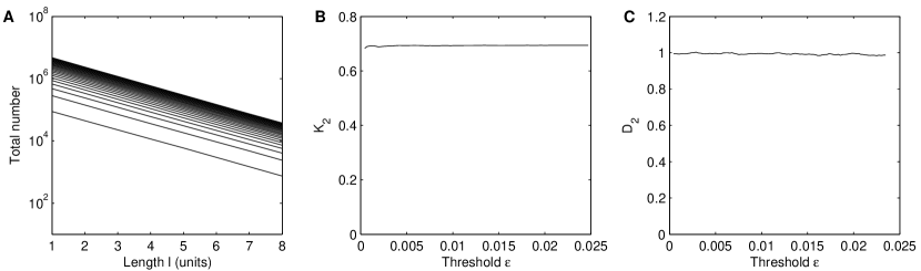
Figure 25: (A) Total number of diagonal lines of at least length $l$ in the RP of the Bernoulli map. Each histogram is computed for a different threshold $\varepsilon$, from 0.000436 (bottom) to 0.0247 (top). 10,000 data points have been used for the computation. (B) Estimate of $K_{2}$ in dependence on $\varepsilon$. (C) Estimate of $D_{2}$ in dependence on $\varepsilon$.

In the case of the Rössler system (Fig. 1B), the most remarkable finding is the existence of two well differentiated scaling regions for the distribution of diagonal lines of at least length $l$ (Fig. 26A): for $1\leq l\leq 84$ the slope is about 3–4 times larger than the slope for $l>84$ (the time interval between two points of the integrated trajectory is 0.2, hence $l=84$ corresponds to 16.8). As $K_{2}$ is defined for $l\to\infty$ the second slope yields the estimation of the entropy, which is $\hat{K}_{2}=0.069\pm 0.003$ (Fig. 26B). Note, that $K_{2}$ is a lower bound for the sum of the positive Lyapunov exponents and the estimated value of $K_{2}$ is close to the largest Lyapunov exponent of the Rössler system, which is approximately 0.072 [121].

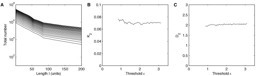
Figure 26: (A) Total number of diagonal lines of at least length $l$ in the RP of the Rössler system. Each histogram is computed for a different threshold $\varepsilon$, from 0.862 (bottom) to 6.465 (top). (B) Estimate of $K_{2}$ in dependence on $\varepsilon$ ($K_{2}=0.069\pm 0.003$). 10,000 data points have been used for the computation. (C) Estimate of $D_{2}$ in dependence on $\varepsilon$ ($D_{2}=2.03\pm 0.03$). 200,000 data points have been used for the computation.

However, the slope of the first part of the curve is interesting too, as it is also independent of $\varepsilon$. The region $1\leq l\leq 84$ characterises the short term dynamics of the system up to three cycles around the attractor and corresponds in absolute units to a time of $t=16.8$. These three cycles reflect a characteristic period of the Rössler system that is called recurrence period $T_{\text{rec}}$. It is different from the dominant phase period $T_{\text{ph}}$, which is given by the dominant frequency of the power spectrum. $T_{\text{rec}}$, however, is given by the recurrences to the same state in phase space.

For predictions on time scales below the recurrence period, the second slope of $\ln(\hat{p}_{c}(\varepsilon,l))$ versus $l$ gives a better predictability than the first slope (more than three times better), which means that there exist two time scales that characterise the attractor. The first slope is greater than the second one because it is more difficult to predict the next step if we have only information about a piece of the trajectory for less than one recurrence period. Once we have scanned the trajectory for more than $T_{\text{rec}}$, the predictability increases and hence, the slope of $p_{c}(\varepsilon,l)$ in the logarithmic plot decreases. Hence the first slope, as well as the time at which the second slope begins, reveal important characteristics of the attractor. Note that even though the first slope is not a dynamical invariant (it changes if one uses embedding coordinates), most of the initial conditions “diverge” at a rate given by the first slope and not by the second one.

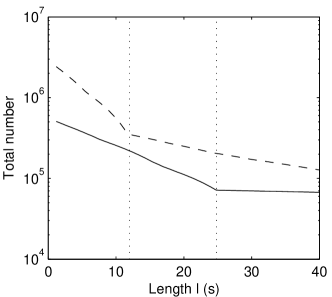
Figure 27: Total number of diagonal lines of at least length $l$ in the RP of the Rössler system with $c=9$ (solid) and $c=30$ (dashed). The two scaling regions are separated at approximately 12 and 24.8, which corresponds to $T_{\text{rec}}=2T_{\text{ph}}$ and $T_{\text{rec}}=4T_{\text{ph}}$, respectively.

The relationship between the transition of the scaling regions and the phase period can also be seen in attractors of different shape. For a Rössler system with fixed $a=b=0.1$, but varied parameter $c$, the form of the attractor as well as $T_{\text{rec}}$ and $T_{\text{ph}}$ change. For example, $c=9$ yields $T_{\text{rec}}=2T_{\text{ph}}$ (with $T_{\text{ph}}\approx 6$), and $c=30$, gives $T_{\text{rec}}=4T_{\text{ph}}$ (with $T_{\text{ph}}\approx 6.2$). In both cases the length of the first scaling region ($T_{\text{rec}}=12$ and $24.8$, resp.) corresponds as expected to $2T_{\text{ph}}$ and $4T_{\text{ph}}$, respectively (Fig. 27). The existence of two scaling regions in the Rössler system is a new and striking point of the recurrence analysis that cannot be observed with the method proposed by Grassberger and Procaccia to estimate $K_{2}$ [110]. The existence of the two different scaling regions can also be found in other non-hyperbolic systems, such as the Lorenz oscillator, Eqs. (• ‣ A). This is an indication of the non-hyperbolic nature of such systems and fits well with results obtained by other approaches [122].

Next, we estimate $D_{2}$ for the Rössler system for various choices of the threshold $\varepsilon$ (Fig. 26D) using Eq. (79) and the average over lines of length $l$ which correspond to the first scaling region. The estimated value using 200,000 data points is $\hat{D}_{2}=1.86\pm 0.04$. This result is in accordance with the estimation of $D_{2}$ by the G-P algorithm given in [123], where the value $1.81$ was obtained. Restricting the average in $l$ to the second scaling region, we obtain the slightly higher value $\hat{D}_{2}=2.03\pm 0.03$, which is in accordance with the value $D_{2}=2.06\pm 0.02$ obtained in [110, 124]. Note that the extent and the onset of a scaling region in $D_{2}(\varepsilon)$ may lead to problems in the $D_{2}$ estimation [125]. Furthermore, the number of points needed to estimate $D_{2}$ accurately is much larger than the one needed for the estimation of $K_{2}$ (in the examples shown here, we used 10,000 data points for the estimation of $K_{2}$ and 200,000 data points for the estimation of $D_{2}$).

Therefore, it is interesting to investigate the dependence of the estimated value for $D_{2}$ on the number of points of the trajectory used for the computation. Let us consider the Bernoulli map and the Rössler system (Fig. 28). We estimate $D_{2}$ by the mean value over 50 different values of the threshold $\varepsilon$ in the same range as in Figs. 25 and  26, respectively. For the Bernoulli map, the estimation of $D_{2}$ is rather accurate for already 10,000 data points. On the other hand, for the Rössler system, at least 50,000 data points are necessary for a more precise estimation. This result confirms the expectation that the higher the dimension or the more complex a system is, the more data points are necessary for its characterisation [46].

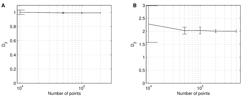
Figure 28: Estimation of $D_{2}$ by means of RPs in dependence on the number of points of the trajectory used for the computation for (A) the Bernoulli map and (B) the Rössler system (second scaling region used). The error bars indicate the standard deviation of $\hat{D}_{2}(\varepsilon)$.

As mentioned at the beginning of this section, it is also possible to estimate the generalised dimensions [111] from the recurrence matrix by

$$D_{q}=\lim_{\varepsilon\to 0}\frac{\log(C_{q}(\varepsilon))}{\log\varepsilon},$$ (84)

with $C_{q}$ given by Eq. (66). The estimation of $D_{q}$ for the simple case of the Bernoulli map reveals $D_{q}\approx 1\ \,\forall\,q$ (Fig. 29), which corresponds to the theoretical value $D_{q}=1\ \,\forall\,q$. However, it must be noted that the problems that arise for the estimation of $D_{q}$ for $q\leq 1$ are also present in the recurrence approach. In order to improve the accuracy of the estimation more sophisticated methods, such as the Enlarged Box Algorithm [126] should be used.

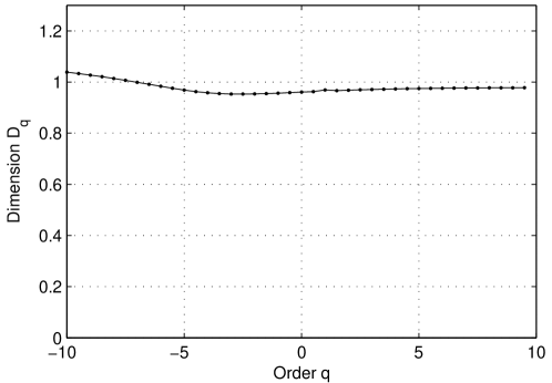
Figure 29: Estimation of $D_{q}$ by means of RPs for the Bernoulli map (20,000 data points have been used for the computation).

3.6.2 Recurrence times and point-wise dimension

Another invariant characteristic, the point-wise dimension, can be also estimated by using recurrence times [34]. Recurrence times can be directly picked up from the RP. First, we denote the set of points of the trajectory $\vec{x}$ which fall into the $\varepsilon$-neighbourhood $B_{\vec{x}_{i}}(\varepsilon)$ of an arbitrary chosen point at $i$ with

$$\mathcal{R}_{i}=\{\vec{x}_{j_{1}},\vec{x}_{j_{2}},\,\dots\,|\ \mathbf{R}_{i,j_{k}}=1\}.$$ (85)

The elements of this set correspond to the recurrence points of the $i^{\text{th}}$ column $\{{\mathbf{R}}_{i,j}\}_{j=1}^{N}$ of an RP. The corresponding recurrence times between these recurrence points (recurrence times of first type, according to the notation given in [34]) are $\{T_{k}^{(1)}=j_{k+1}-j_{k}\}_{k\in\mathds{N}}$. Due to possible tangential motion, some of the recurrence points in $\mathcal{R}_{i}$ correspond to recurrence times $T_{k}^{(1)}=1$ (Fig. 21). However, in order to obtain the real recurrence times (Poincaré recurrence times), such points must be discarded. One approach is to remove all consecutive recurrence points with $T_{k}^{(1)}=1$ from the set $\mathcal{R}_{i}$. This results in a new set $\mathcal{R}^{\prime}_{i}=\{\vec{x}_{j^{\prime}_{1}},\vec{x}_{j^{\prime}_{2}},\dots\}$. Then, the recurrence times (recurrence times of second type according to [34]) $\{T_{k}^{(2)}=j^{\prime}_{k+1}-j^{\prime}_{k}\}_{k\in\mathds{N}}$ are calculated from the remaining recurrence points (i. e. from $\mathcal{R}^{\prime}_{i}$). Hence, $T^{(2)}$ measures vertically the time distance between the beginning of (vertically) subsequent recurrence structures in the RP. An alternative estimator for the recurrence times $T^{(2)}$ is the average of the lengths of the white vertical lines at a specific column of the RP. For systems with less laminar structures in the RP (i. e. $LAM$ and $TT$ tend to zero), the distribution of such an average almost coincides with the distribution of $T^{(2)}$ as defined by [34]. However, for systems with laminar states (e. g. logistic map for certain values of the control parameter), $T^{(2)}$ as defined by [34] over-estimates the recurrence times and $T^{(2)}$ computed from the white vertical lines under-estimates the recurrence times.

Based on the recurrence times $T^{(1)}$ and $T^{(2)}$, it is possible to estimate the point-wise dimension $D_{P}(i)$, which is defined by

$$\mu\left(B_{\vec{x}_{i}}(\varepsilon)\right)\sim\varepsilon^{D_{P}(i)},$$ (86)

where $\mu\left(\cdot\right)$ is the probability measure (cf. Eq. (2)). The measure $\mu\left(B_{\vec{x}_{i}}(\varepsilon)\right)$ can be estimated by the frequency at which the neighbourhood of the point at $i$ is visited by the trajectory, which is the reciprocal of the mean recurrence time $\langle T^{(1)}\rangle$, i. e. $\mu\left(B_{\vec{x}_{i}}(\varepsilon)\right)=\mu\left(\mathcal{R}_{i}\right)\approx 1/\langle T^{(1)}\rangle$ and thus [34]

$$\langle T^{(1)}(\varepsilon)\rangle\sim\varepsilon^{-D_{P}(i)}.$$ (87)

This measure depends on the chosen point $\vec{x}_{i}$, because some parts of the attractor are visited more frequently than others.

Analogously, we can state that the measure of the set of neighbours of $\vec{x}_{i}$ without points belonging to the tangential motion $\mathcal{R}^{\prime}_{i}$ is $\mu(\mathcal{R}^{\prime}_{i})\approx 1/\langle T^{(2)}\rangle$. When the points belonging to the tangential motion represent a zero-dimensional set, $\mu(\mathcal{R}^{\prime}_{i})=\mu(\mathcal{R}_{i})\sim\varepsilon^{D_{P}(i)}$. When these points represent a one-dimensional set, $\mu(\mathcal{R}^{\prime}_{i})\sim\varepsilon^{D_{P}(i)-1}$. Hence, for discrete maps and continuous systems with small $\varepsilon$,

$$\langle T^{(2)}(\varepsilon)\rangle\sim\varepsilon^{-D_{P}(i)},$$ (88)

and for continuous systems with large $\varepsilon$,

$$\langle T^{(2)}(\varepsilon)\rangle\sim\varepsilon^{-(D_{P}(i)-1)}.$$ (89)

Furthermore, the mean recurrence times can be used to analyse transient and non-stationary dynamics, computing them in sliding windows and monitoring how $\langle T^{(1)}(\varepsilon)\rangle$ and $\langle T^{(2)}(\varepsilon)\rangle$ change in different blocks of sub-data sets. When analysing experimental data, often only scalar time series are available. Hence, the time delay embedding technique must be used. In this case, the disadvantage of using $\langle T^{(1)}(\varepsilon)\rangle$ to analyse the non-stationarity, is that it sensitively depends on the used embedding parameters. Hence, in this case $\langle T^{(2)}(\varepsilon)\rangle$ yields more robust results.

3.6.3 Generalised mutual information (generalised redundancies)

The mutual information quantifies the amount of information that we obtain from the measurement of one variable on another. It has become a widely applied measure to quantify dependencies within or between time series (auto and cross mutual information). The time delayed generalised mutual information (redundancy) $I_{q}(\tau)$ of a system $\vec{x}_{i}$ is defined by [119]

$$I_{q}^{\vec{x}}(\tau)=2H_{q}-H_{q}(\tau).$$ (90)

$H_{q}$ is the $q^{\text{th}}$-order Rényi entropy of $\vec{x}_{i}$ and $H_{q}(\tau)$ is the $q^{\text{th}}$-order joint Rényi entropy of $\vec{x}_{i}$ and $\vec{x}_{i+\tau}$

$$H_{q}=-\ln\sum\limits_{k}p_{k}^{q},\qquad H_{q}(\tau)=-\ln\sum\limits_{k,l}p_{k,l}^{q}(\tau),$$ (91)

where $p_{k}$ is the probability that $\vec{x}_{i}$ is in the $k^{\text{th}}$ box and $p_{k,l}(\tau)$ is the joint probability that $\vec{x}_{i}$ is in box $k$ and $\vec{x}_{i+\tau}$ is in box $l$ (note that we use here the same neighbourhood definition as for Eq. (68)). Assuming that the system under consideration is ergodic and approximating the probability that $\vec{x}_{i}$ is in the $k^{\text{th}}$ box of the partition by the probability to find a point of the trajectory in a box of size $\varepsilon$ centred at $\vec{x}_{i}$, the recurrence matrix can be used to estimate Eq. (91) in the case $q=2$,

$$\hat{H}_{2}=-\ln\left(\frac{1}{N^{2}}\sum_{i,j=1}^{N}\mathbf{R}_{i,j}\right)$$ (92)

and

$$\hat{H}_{2}(\tau)=-\ln\left(\frac{1}{N^{2}}\sum_{i,j=1}^{N}\mathbf{R}_{i,j}\mathbf{R}_{i+\tau,j+\tau}\right)=-\ln\left(\frac{1}{N^{2}}\sum_{i,j=1}^{N}\mathbf{JR}^{\vec{x},\vec{x}}_{i,j}(\tau)\right),$$ (93)

where $\mathbf{JR}^{\vec{x},\vec{x}}_{i,j}(\tau)$ denotes the delayed joint recurrence matrix, Eq. (40). The second order generalised mutual information can be estimated then by means of RPs [115]

$$\hat{I}_{2}^{\vec{x}}(\tau)=\ln\left(\frac{1}{N^{2}}\sum\limits_{i,j=1}^{N}\mathbf{JR}_{i,j}^{\vec{x},\vec{x}}(\tau)\right)-2\ln\left(\frac{1}{N^{2}}\sum\limits_{i,j=1}^{N}\mathbf{R}_{i,j}\right).$$ (94)

As mentioned in the introduction of this section, the mutual information can be estimated by means of the correlation sum [127]. The joint distribution can be considered as the distribution in a two-dimensional embedding space [73]. Hence,

$$\tilde{I}_{2}^{\vec{x}}(\tau)=\ln C_{2}^{\tau}(\varepsilon)-2\ln C_{2}(\varepsilon),$$ (95)

where $C_{2}^{\tau}(\varepsilon)$ is the correlation dimension of the embedded two dimensional vectors $\vec{x}_{i}(\tau)=(u_{i},u_{i+\tau})^{T}$, and $C_{2}(\varepsilon)$ is the correlation sum of the scalar time series $u_{i}$. This corresponds to Eq. (94) in the special case that the dimension of $\vec{x}$ is equal to one (i. e. that it is a scalar time series) and for the maximum norm (Fig. 30A). The advantage using the RP approach is that we can compute the mutual information for an entire phase space vector and not only for a single component.

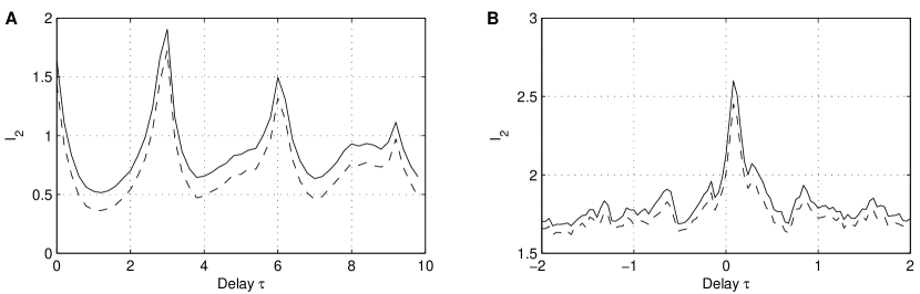
Figure 30: (A) Mutual information for the $x$-component of the Rössler system, Eqs. (• ‣ A), with $a=0.15$, $b=0.2$ and $c=10$, and time step $\Delta t=0.2$, computed by the RP method (solid line) and the correlation sum approach (dashed line). (B) Cross mutual information between the $x$ and $y$-components of the Lorenz system, Eqs. (• ‣ A), for $\sigma=10$, $b=\frac{5}{3}$ and $r=28$ and time step $\Delta t=0.04$, computed by the RP method (solid line) and the correlation sum approach (dashed line). The difference between the two estimations is due to the used Euclidean norm; using the maximum norm, both curves coincide.

Moreover, the generalised cross mutual information of second order of two different systems $\vec{x}$ and $\vec{y}$

$$I_{2}^{\vec{x},\vec{y}}=H_{2}^{\vec{x}}+H_{2}^{\vec{y}}-H_{2}^{\vec{x},\vec{y}}.$$ (96)

can be estimated by means of RPs as well:

$$\hat{I}_{2}^{\vec{x},\vec{y}}=-\ln\frac{1}{N^{2}}\sum_{i,j=1}^{N}\mathbf{R}_{i,j}^{\vec{x}}-\ln\frac{1}{N^{2}}\sum_{i,j=1}^{N}\mathbf{R}_{i,j}^{\vec{y}}+\ln\frac{1}{N^{2}}\sum_{i,j=1}^{N}\mathbf{JR}^{\vec{x},\vec{y}}_{i,j}.$$ (97)

However, $\hat{I}_{2}^{\vec{x},\vec{y}}$ depends on the special choices of the thresholds $\varepsilon^{\vec{x}}$ and $\varepsilon^{\vec{y}}$. If, e. g., the phase space diameter of $\vec{x}$ is very large in comparison with the one of $\vec{y}$, then the value for $\varepsilon^{\vec{x}}$ should be chosen larger than the value for $\varepsilon^{\vec{y}}$. One possibility to equilibrate the difference between the sizes of both phase spaces is to choose the thresholds in such a way that the recurrence rate of $\vec{x}$ is equal to the recurrence rate of $\vec{y}$ (as described in Subsec. 3.2.2), i. e.

$$\frac{1}{N^{2}}\sum_{i,j=1}^{N}\mathbf{R}_{i,j}^{\vec{x}}=\frac{1}{N^{2}}\sum_{i,j=1}^{N}\mathbf{R}_{i,j}^{\vec{y}}=RR.$$ (98)

Then, the estimate of $I_{2}^{\vec{x},\vec{y}}$ can be written as

$$\tilde{I}_{2}^{\vec{x},\vec{y}}=\ln\frac{1}{N^{2}}\sum_{i,j=1}^{N}\mathbf{JR}_{i,j}-2\ln RR.$$ (99)

Using the delayed joint recurrence matrix, Eq. (40), the cross mutual information can be computed as a function of the time delay (Fig. 30B). The cross mutual information is also called cross redundancy [113].

3.6.4 Influence of embedding on the invariants estimated by RPs

We have seen in the last subsections, that it is possible to estimate basic dynamical invariants by means of RPs. As usually in nonlinear time series analysis, if the time evolution of only one component of the state vector is observed, the trajectory in the phase space has to be reconstructed by means of an appropriate embedding before computing the dynamical invariants (cf. Subsec. 3.1). However, we show in this section, that this additional step is not necessary for the estimation of $K_{2}$ and $D_{2}$ by means of RPs.

As we have shown in Subsec. 3.6.1, the estimation of $K_{2}$ and $D_{2}$ is based on the probability $p_{c}(\varepsilon,l)$ to find a diagonal of at least length $l$ in an RP. Using embedded vectors, Eq. (9), with embedding dimension $m$ and delay $\tau$, and considering the maximum norm for the estimation of $p_{c}(\varepsilon,l)$, we get

$$p_{c}^{(m,\tau)}(\varepsilon,l)=\frac{1}{N^{2}}\sum\limits_{i,j=1}^{N}\prod\limits_{k=0}^{l-1}\Theta\left(\varepsilon-\max\limits_{s=0,\ldots,m-1}\left|x_{i+k+s\tau}-x_{j+k+s\tau}\right|\right).$$ (100)

The product in Eq. (100) can be written as

$$\begin{split}\prod\limits_{k=0}^{l-1}\Theta\bigl{(}\varepsilon-\max\limits_{s=0,\ldots,m-1}\left|x_{i+k+s\tau}-x_{j+k+s\tau}\right|\bigr{)}=\\ \Theta\bigl{(}\varepsilon-\max\limits_{m=0,\cdots,l-1\atop s=0,\ldots,m-1}\left|x_{i+k+s\tau}-x_{j+k+s\tau}\right|\bigr{)}.\end{split}$$ (101)

Hence, substituting this into Eq. (100), we obtain

$$p_{c}^{(m,\tau)}(\varepsilon,l)=\frac{1}{N^{2}}\sum\limits_{i,j=1}^{N}\Theta\left(\varepsilon-\max\limits_{k=0,\ldots,\atop l-1+(m-1)\tau}\left|x_{i+k}-x_{j+k}\right|\right).$$ (102)

From this equation it follows that for different embedding $(m,\tau)$ and $(m^{\prime},\tau^{\prime})$ the following relationship holds

$$p_{c}^{(m,\tau)}(\varepsilon,l)=p_{c}^{(m^{\prime},\tau^{\prime})}(\varepsilon,l^{\prime})\quad\text{if}\quad l+(m-1)\tau=l^{\prime}+(m^{\prime}-1)\tau^{\prime},$$ (103)

provided that $l,l^{\prime}>\tau,\tau^{\prime}$ and $m,m^{\prime}\geq 1$ [116]. Hence, the decay of $p_{c}^{(m,\tau)}(\varepsilon,l)$ is the same for different embedding. The curve is only shifted to larger $l$’s if the dimension is decreased. Since the slope of $\ln p_{c}^{(m,\tau)}(\varepsilon,l)$ for large $l$’s is used in order to the estimate $K_{2}$ (see Subsec. 3.6.1), the estimated value is independent of the choice of the embedding parameters.

Analogously, substituting

$$\ln\left(\frac{p_{c}^{(d,\tau)}(\varepsilon_{1},l)}{p_{c}^{(d,\tau)}(\varepsilon_{2},l)}\right)=\ln\left(\frac{p_{c}^{(d^{\prime},\tau)}(\varepsilon_{1},l^{\prime})}{p_{c}^{(d^{\prime},\tau)}(\varepsilon_{2},l^{\prime})}\right)$$ (104)

in Eq. (79), we see that the estimation of $D_{2}$ by means of RPs is also independent of the choice of the embedding parameters. Hence, this is one important advantage of the RPs method compared to others.

3.7 Extension to spatial data

The concept of recurrence is not only restricted to univariate time series. It is clear that recurrence is also a basic phenomenon in spatio-temporal dynamical systems. But even for snapshots of such high-dimensional dynamics, such as images, we can expect recurrent structures. However, RPs cannot be directly applied to spatial data. One possibility to study the recurrences of spatial data is to separate these objects into many one-dimensional data series, and to apply the recurrence analysis separately to each of these series [128]. Another possibility, suggested in this section, is the extension of the temporal approach of RPs to a spatial one [129]. With this step we focus on the RPs’ potential to determine similar (recurrent) epochs in data.

For a $d$-dimensional (Cartesian) space, we define a spatial recurrence plot by

$$\mathbf{R}_{\vec{\imath},\vec{\jmath}}=\Theta\left(\varepsilon-\left\|\vec{x}_{\vec{\imath}}-\vec{x}_{\vec{\jmath}}\right\|\right),\quad\vec{x}_{\vec{\imath}}\in\mathds{R}^{m},\ \vec{\imath},\,\vec{\jmath}\in\mathds{N}^{d},$$ (105)

where $\vec{\imath}$ is the $d$-dimensional coordinate and $\vec{x}_{\vec{\imath}}$ is the phase-space vector at the location given by coordinate $\vec{\imath}$. This means, we consider each direction in space as a single embedding vector of dimension $m$, but compare each of them with all others. The resulting RP has now the dimension $2\times d$ and cannot be visualised anymore. However, its quantification is still possible.

Analogously to the one-dimensional case, where the LOI is a one-dimensional line (Subsec. 3.2.1), a similar diagonal-oriented, $d$-dimensional structure in the $n$-dimensional recurrence plot ($n=2\,d$), the hyper-surface of identity (HSOI), can be defined:

$$\mathbf{R}_{\vec{\imath},\vec{\jmath}}\equiv 1\quad\forall\ \vec{\imath}=\vec{\jmath}.$$ (106)

In the special case of a two-dimensional image with scalar values instead of phase-space vectors, i. e. $m=1$, we have

$$\mathbf{R}_{i_{1},i_{2},j_{1},j_{2}}=\Theta\left(\varepsilon-\left|x_{i_{1},i_{2}}-x_{j_{1},j_{2}}\right|\right),$$ (107)

which is in fact a four-dimensional recurrence plot, and its HSOI is a two-dimensional plane.

In two-dimensional RPs, the recurrence quantification is based on line structures. Thus, the definition of equivalent structures in higher-dimensional RPs is crucial for their quantification analysis.

Analogously to the definition of diagonal lines, Eq. (14), a diagonal hyper-surface of size $l$ ($\vec{l}=(l,\dots,l),\vec{l}\in\mathds{N}^{d}$) is then defined by

$$\left(1-\mathbf{R}_{\vec{\imath}-\vec{1},\vec{\jmath}-\vec{1}}\right)\left(1-\mathbf{R}_{\vec{\imath}+\vec{l},\vec{\jmath}+\vec{l}}\right)\prod_{\begin{subarray}{c}k_{1},\dots,k_{d}=0\end{subarray}}^{l-1}\mathbf{R}_{\vec{\imath}+\vec{k},\vec{\jmath}+\vec{k}}\equiv 1,$$ (108)

and a vertical hyper-surface of size $v$ ($\vec{v}=(v,\dots,v),\vec{v}\in\mathds{N}^{d}$) is given by

$$\left(1-\mathbf{R}_{\vec{\imath},\vec{\jmath}-\vec{1}}\right)\left(1-\mathbf{R}_{\vec{\imath},\vec{\jmath}+\vec{v}}\right)\prod_{\begin{subarray}{c}k_{1},\dots,k_{d}=0\end{subarray}}^{v-1}\mathbf{R}_{\vec{\imath},\vec{\jmath}+\vec{k}}\equiv 1.$$ (109)

Using these definitions, we can compute the frequency distributions of the sizes of diagonal and vertical hyper-surfaces in the spatial RP. The recurrence quantification measures, as defined in Subsec. 3.5, can be applied to these distributions, and hence, these quantification measures are now suitable for characterising spatial data as well.

Example: RQA of spatial data

To illustrate the extension of temporal RPs to higher-dimensional spatial RPs, we consider three prototypical examples in 2D (i. e. images). The first image (A) is uniformly distributed white noise, the second image (B) is the result of a static two-dimensional auto-regressive process (2${}^{\text{nd}}$ order, AR2), Eq. (126), and the third image (C) represents periodically recurrent structures (Fig. 31). All these examples have a geometric size of $200\times 200$ pixels, and the values of the spatial series are normalised to a mean of zero and a standard deviation of one.

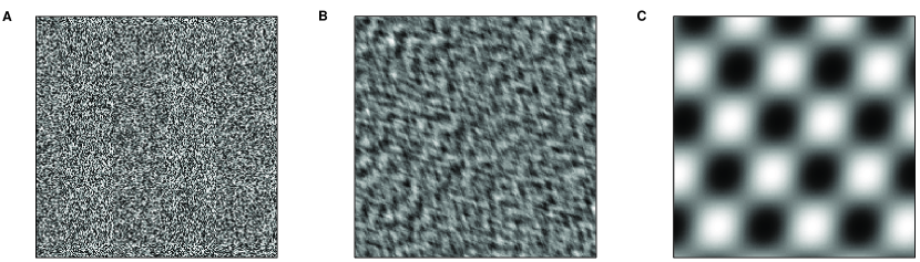
Figure 31: Two-dimensional examples representing (A) uniformly distributed white noise, (B) a two-dimensional auto-regressive process and (C) periodically recurring structures.

The resulting RPs are four-dimensional matrices of size $200\times 200\times 200\times 200$, and can hardly be visualised. However, we can reduce their dimension by one in order to visualise these RPs: we consider only that part of the RP, where $i_{2}=j_{2}$ (the resulting $200\times 200\times 200$ cube is a hyper-surface of the four-dimensional RP along the LOI).

The features obtained in higher-dimensional RPs can be interpreted analogously to the case of two-dimensional RPs. Single points correspond to strongly fluctuating, uncorrelated data, as it is typical for noise (Fig. 32A). Correlations in the data cause extended structures, which can be lines, planes or even cuboids (Fig. 32B). Periodically recurrent patterns in data induce periodic line and plane structures in the spatial RP (Fig. 32C).

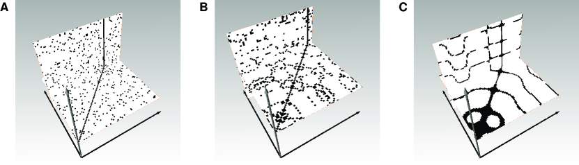
Figure 32: Slices through three-dimensional subsections of four-dimensional RPs of the two-dimensional examples shown in Fig. 31. As known from one-dimensional data, (A) random data causes homogeneous RPs consisting of single points, (B) correlations in data cause extended structures and (C) periodic data causes periodically occurring structures in the RPs ($\varepsilon=0.2$)

The recurrence quantification of these 4D RPs confirms these observations. Except from the recurrence rate $RR$, the other recurrence quantification measures discriminate clearly between the three features (Tab. 3). Because all images were normalised to the same standard deviation, the recurrence rate $RR$ is roughly the same for all examples. For the random image (A) the determinism $DET_{HS}$ and laminarity $LAM_{HS}$ tend to zero, what is expected, because the values in the image heavily fluctuate even between adjacent pixels. For the 2D-AR2 image (B), $DET_{HS}$ and $LAM_{HS}$ are slightly above zero, revealing the correlation between adjacent pixels. The last example (C) has, as expected, the highest values in $DET_{HS}$ and $LAM_{HS}$, because same structures occur several times in this image and the image is rather smooth. Although the variation in $DET_{HS}$ and $LAM_{HS}$ seems to be similar, there is a significant difference between both measures. Whereas $LAM_{HS}$ represents the probability that a specific value will not change over spatial variation (what results in extended same-coloured areas in the image), $DET_{HS}$ measures the probability that similar changes in the image recur. The value obtained for $LAM_{HS}$ is twice the one obtained for $DET_{HS}$ in the 2D-AR2 image. Hence, there are more areas without changes in the image than such with typical, recurrent changes. In contrast, $DET_{HS}$ is higher than $LAM_{HS}$ for the periodic image, because it contains characteristic changing structures which recur several times but do not have a constant value.

Table 3: Recurrence quantification measures for prototypical examples in 2D. For the minimal size of the diagonal and vertical planes $l_{min}=3$ and $v_{min}=4$ is used.

Example	$RR$	$DET$	$LAM$
(A) noise	0.218	0.007	0.006
(B) 2D-AR2	0.221	0.032	0.065
(C) periodic	0.219	0.322	0.312

3.8 Synchronisation analysis by means of recurrences

In this section, the relationship between recurrences and synchronisation of complex systems will be discussed. This relationship can be used in order to detect different transitions to synchronisation and also to detect synchronisation in cases where known methods fail.

There are three basic types of synchronisation in coupled complex systems: if the trajectories of the systems evolve due to coupling on the same trajectory, they are completely synchronised. If there exists a functional relationship between the systems, they are generalised synchronised, and if their phases adapt to each other so that they evolve in the same manner, the systems are phase synchronised.

If two systems synchronise in some way, their recurrences in phase space are not independent from each other. Hence, comparing the recurrences of each single system with the joint recurrences of the entire system, we can expect to get indications about their synchronisation type and degree.

On the other hand, RPs reflect the different time scales which play a crucial role in the dynamics of a system. For example, the RP of a periodic trajectory (Fig. 1A) consists of uninterrupted diagonal lines equally spaced. The distance between the diagonal lines is the period of the trajectory. In the case of white noise (Fig. 1C), the RP consists of mostly isolated points uniformly distributed, thus, the distances between the recurrence points are uniformly distributed, indicating that there is no predominant time scale in the series. Hence, there is an equivalence between the distances which separate the recurrent points in the RP and the characteristic time scales of the considered system. This correspondence is crucial in order to analyse phase synchronisation, where the phases or time scales of the interacting systems are locked.

In this section, we give first a brief overview about synchronisation of chaotic systems. Then, the detection of different kinds of transitions to synchronisation by means of joint recurrences is presented. At last, some indices for the detection of phase and generalised synchronisation based on recurrences are introduced.

3.8.1 Synchronisation of chaotic systems

Chaotic systems defy the concept of synchronisation due to the high sensitivity to slightly different initial conditions. However, it has been demonstrated that this kind of systems can synchronise.

The first studies about synchronisation of chaotic systems consider complete synchronisation (CS). In this case, coupled identical chaotic systems which start at different initial conditions evolve onto the same trajectory [130, 131, 132]. However, under experimental conditions it is difficult and mostly impossible to have two fully identical systems. Usually, there is some mismatch between the parameters of the systems under consideration. Hence, it is important to study synchronisation between non-identical systems. Starting with two uncoupled non-identical oscillators and increasing the coupling strength, a rather weak degree of synchronisation may occur, where the phases and frequencies of the chaotic oscillators become locked, whereas their amplitudes often remain almost uncorrelated. This behaviour is denoted by phase synchronisation (PS).

The phase of a chaotic autonomous oscillator is closely related to its zero Lyapunov exponent because it corresponds to the translation along the chaotic trajectory. Hence, a perturbation in this direction neither decays nor grows. This property makes the adjustment of the phases of two chaotic oscillators (or of one oscillator and a force) possible. If two chaotic oscillators are not coupled, the two zero Lyapunov exponents will be linked to the individual phases. Increasing the coupling strength, PS can be obtained by the transition of one of the zero Lyapunov exponents to negative values, indicating the establishment of a relationship between the phases [133].

If the coupling strength between non-identical chaotic oscillators is further increased, a strong dependence between the amplitudes will then be established, so that the states of both oscillators become almost identical but shifted in time, i. e. $\vec{x}(t)\approx\vec{y}(t+\tau)$ [99]. This regime is called lag synchronisation (LS). The transition to LS has also been related to the transition of a positive Lyapunov exponent to negative values. Actually, LS sets in after the zero crossing of the Lyapunov exponent. After the onset of LS, a further increase of the coupling strength leads to a decrease of the time lag $\tau$ between the trajectories of the oscillators. Hence, the oscillators tend to be almost synchronised, i. e. $\vec{x}(t)\approx\vec{y}(t)$.

Note that the above descriptions of synchronisation transitions and their connection with the changes in the Lyapunov spectrum is valid for phase coherent oscillators, for which a phase can be defined as a monotonously increasing function of time. However, for non-phase coherent chaotic oscillators, this definition may not be possible and the crossing of the zero Lyapunov exponent to negative values may not be an indicator for the onset of PS [134].

The question about synchronisation of coupled systems which are essentially different has been addressed first in [131, 135]. In this case, there is in general no trivial manifold in phase space which attracts the systems’ trajectories. It has been shown, that these systems can synchronise in a more general way, namely $\vec{y}=\vec{f}(\vec{x})$, where $\vec{f}$ is a transformation which maps asymptotically the trajectories of $\vec{x}$ into the ones of the attractor $\vec{y}$, leading to generalised synchronisation (GS). The properties of the function $\vec{f}$ depend on the features of the systems $\vec{x}$ and $\vec{y}$, as well as on the attraction properties of the synchronisation manifold $\vec{y}=\vec{f}(\vec{x})$. In most cases, evidence of GS has been provided for unidirectional coupling schemes. However, examples of bidirectionally coupled systems that undergo GS also exist, as e. g. shown in [136, 137].

All these different types of synchronisation between complex systems have been demonstrated in numerous laboratory experiments [132, 138, 139, 140, 141, 142, 143] and in natural systems [144, 145, 146].

3.8.2 Detection of synchronisation transitions

As we have seen in Subsec. 3.6, it is possible to estimate the joint Rényi entropy by means of JRPs (cf. Eq. (83)). In this section, the transitions to PS and LS will be characterised by means of the joint Rényi entropy. To exemplify this, we consider the prototypical chaotic system of two mutually coupled Rössler oscillators, Eqs. (• ‣ A) and (• ‣ A) with $a=0.15$, $b=0.20$, $c=10$, for the coupling parameters $\nu\in[-0.04,0.04]$ and $\mu\in[0.0,0.12]$, for which the two oscillators undergo transitions to PS. The difference of the mean frequencies $\Delta\Omega=\Omega_{1}-\Omega_{2}$ of both oscillators reveals the well-known Arnold tongue (Fig. 33; the mean frequencies $\Omega_{1}$ and $\Omega_{2}$ are calculated as proposed in [133]).

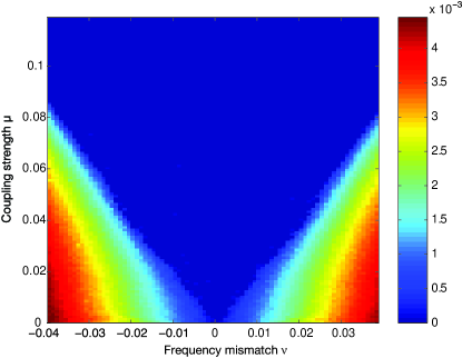
Figure 33: The difference $|\Delta\Omega|$ between the mean frequencies of two Rössler oscillators in dependence on the frequency mismatch $\nu$ and coupling strength $\mu$ shows the well-known Arnold tongue [147].

Next, we estimate $JK_{2}$ based on JRPs, Eq. (83), in the same parameter range for both oscillators. The results also reflect the Arnold tongue (Fig. 34A), but exhibit more details than $\Delta\Omega$ (Fig. 33).

• First, two “borders” in the upper part of the plot can be observed ($\mu>0.04$): the outer one corresponds to the border of the Arnold tongue, i. e. inside this border the oscillators are in PS, whereas outside they are not. Both borders have very low values of $\widehat{JK_{2}}$, i. e. the behaviour of the system is rather regular there, even periodic in small regions on both borders. This is a remarkable fact, because it means that for relatively high coupling strengths the transition to PS is chaos-period-chaos, since inside the tongue is $\widehat{JK}_{2}>0$, indicating a chaotic regime.

• Inside the Arnold tongue, for coupling strengths $\mu$ between approximately $0.025$ and $0.04$, a region can be found (which looks like two eyes), where the value of $\widehat{JK}_{2}$ is (almost) zero, i. e. the region is periodic or quasi-periodic.

• For $\mu\geq 0.03$ the region inside the Arnold tongue is “more chaotic” (larger $\widehat{JK}_{2}$) than outside the tongue. This is surprising, as we would expect that if both oscillators are synchronised, the behaviour of the whole system becomes more and more regular for increasing coupling.

Hence, by means of $JK_{2}$ estimated by recurrences, new characteristics of the transition to PS can be found.

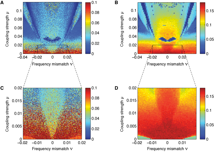
Figure 34: (A) Estimate of the joint Rényi entropy $\widehat{JK}_{2}$ of two Rössler oscillators in dependence on the frequency mismatch $\nu$ and coupling strength $\mu$. (B) Sum of the positive Lyapunov exponents of the two Rössler oscillators in dependence on the frequency mismatch $\nu$ and coupling strength $\mu$. (C) and (D) magnifications of the joint Rényi entropy (C) and the sum of the positive Lyapunov exponents (B) for low values of the coupling strength: The tip of the Arnold tongue cannot be clearly distinguished by the sum of the positive Lyapunov exponents, but by the joint Rényi entropy [147].

In order to validate these results, the formal relationship between $K_{2}$ and the Lyapunov exponents, Eq. (67), can be used. As two coupled systems can be regarded as a single system, the joint Rényi entropy corresponds to the Rényi entropy of the whole system. Therefore, Eq. (67) is also valid for $JK_{2}$, considering the sum over the positive Lyapunov exponents of both sub-systems.

We calculate the Lyapunov spectrum of the whole system defined by Eqs. (• ‣ A) and (• ‣ A), by using the equations (i. e. not estimated from the time series). As $JK_{2}$ is bounded from above by the sum of the positive Lyapunov exponents, Eq. (67), the plot of $\sum_{\lambda_{i}>0}\lambda_{i}$ shows qualitatively the same structures as the plot of $\widehat{JK}_{2}$ (Fig. 34A, B). It is noteworthy, that $JK_{2}$ was estimated from the time series of both oscillators, consisting of $10,000$ data points and with a sampling rate corresponding to $30$ data points per oscillation, whereas for the computation of the sum of the positive Lyapunov exponents, Eqs. (• ‣ A) and (• ‣ A) were used [147]. Hence, the technique to estimate the predictability of the system in parameter space based on JRPs is quite appropriate and yields robust and reliable results even in cases, where the equations governing the system are not known.

However, there is one qualitative difference between both approaches: for $\mu\in[0,0.006]$ the tip of the Arnold tongue can be clearly identified by $\widehat{JK}_{2}$, but it cannot be distinguished by considering the sum of the positive Lyapunov exponents (Fig. 34C, D). This is due to the fact, that the equality $K_{2}=\sum_{\lambda_{i}>0}\lambda_{i}$ holds only for hyperbolic systems, but the 6-dimensional system, Eqs. (• ‣ A) and (• ‣ A), is not hyperbolic, and hence only the relation (67) holds. Hence, $JK_{2}$ provides important complementary information to the sum of the positive Lyapunov exponents.

3.8.3 Detection of PS by means of recurrences

In order to detect phase synchronisation (PS), now we use the relationship between the (vertical) distances which separate diagonal lines in an RP, and the time scales which characterise the dynamical system.

The straightforward procedure to detect PS in complex oscillators is to estimate explicitly their phases. If the system has a dominant peak in the power spectrum, there are several methods to define the phase. One possibility is to project the trajectory on an appropriate plane, so that the projection looks like a smeared limit cycle with well-defined rotations around a centre (Fig. 35A). Then the phase can be identified with the angle of rotation [148, 133]

$$\Phi(t)=\arctan\frac{y(t)}{x(t)}.$$ (110)

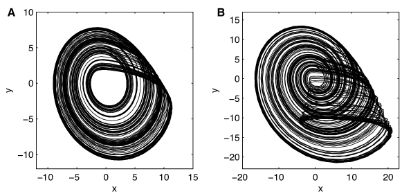
Figure 35: (A) Projection of the Rössler attractor, Eqs. (• ‣ A), with $a=0.15$, $b=0.2$ and $c=10$, on the $(x,y)$-plane. It looks like a smeared limit cycle. Hence, a phase can be assigned to the chaotic oscillator just by means of the angle of rotation around the fixed point, Eq. (110). (B) Projection of the Rössler attractor in the funnel regime, Eqs. (• ‣ A), with $a=0.3$, $b=0.4$ and $c=7.5$, on the $(x,y)$-plane. There is no point around which the trajectory oscillates. Hence, the definition of the phase by Eq. (110) is not appropriate in this case.

But a pre-requisite for the appropriate application of these techniques is that the trajectory in a certain projection plane moves around an origin. This condition may not be met if the signal has a broad-band spectrum, which is typical for non-coherent signals (Fig. 35B) [148, 133, 149].

One approach to overcome this problem is to use an ensemble of well-defined oscillators which act as a filter to find out the frequency of the complex signal [149]. However, depending on which coordinate used to couple the complex system to the ensemble of oscillators, the value obtained for the frequency can vary. Another definition of the phase, based on the general idea of the curvature, has recently been proposed to treat such systems, e. g., the Rössler system in the non-coherent funnel regime [150]. However, this approach is in general limited to lower dimensional systems and is rather sensitive to high levels of noise.

Alternatively, the concept of recurrence can be used to detect indirectly PS in a wide class of chaotic systems and even for time series corrupted by noise, where other methods fail [151]. As demonstrated in Subsec. 3.5.2, diagonal lines in the RP indicate the existence of some determinism in the system under consideration. The vertical distances between these diagonal lines reflect the characteristic time scales of the system. In contrast to periodic dynamics, for a chaotic oscillator the diagonal lines are interrupted due to the divergence of nearby trajectories. Furthermore, the distances between the diagonal lines are not constant, i. e. we find a distribution of distances, reflecting the different time scales present in the chaotic system (Fig. 36).

If two oscillators are in PS, the distances between diagonal lines in their respective RPs coincide, because their phases, and hence their time scales adapt to each other. However, the amplitudes of oscillators, which are only PS but not in GS or CS, are in general uncorrelated. Therefore, their RPs are not identical. However, if the probability that the first oscillator recurs after $\tau$ time steps is high, then the probability that the second oscillator recurs after the same time interval will be also high, and vice versa. Therefore, looking at the probability $p(\varepsilon,\tau)$ that the system recurs to the $\varepsilon$-neighbourhood of a former point $\vec{x}_{i}$ of the trajectory after $\tau$ time steps and comparing $p(\varepsilon,\tau)$ for both systems allows detecting and quantifying PS properly. $p(\varepsilon,\tau)$ can be estimated directly from the RP by using the diagonal-wise calculated $\tau$-recurrence rate, Eq. (50),

$$\hat{p}(\varepsilon,\tau)=RR_{\tau}(\varepsilon)=\frac{1}{N-\tau}\sum_{i=1}^{N-\tau}\Theta(\varepsilon-\|\vec{x}_{i}-\vec{x}_{i+\tau}\|).$$ (111)

As already stated in Subsec. 3.5.2, $\hat{p}(\varepsilon,\tau)$ can be considered as a generalised auto-correlation function, revealing also higher order correlations between the points of the trajectory in dependence on $\tau$. In order to simplify the notation, henceforth we will use $p(\tau)$ instead of $\hat{p}(\varepsilon,\tau)$.

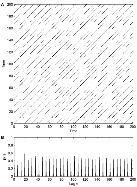
Figure 36: (A) RP of the Rössler system, Eqs. (• ‣ A), for $a=0.15$, $b=0.2$ and $c=10$. (B) Corresponding probability of recurrence $p(\tau)$, i. e. $RR_{\tau}$.

Studying the coincidence of the positions of the maxima of $p_{\tau}$ for two coupled systems $\vec{x}$ and $\vec{y}$, PS can be identified. More precisely, the correlation coefficient between $p_{\tau}^{\vec{x}}$ and $p^{\vec{y}}(\tau)$

$$CPR=\langle\bar{p}^{\vec{x}}(\tau)\bar{p}^{\vec{y}}(\tau)\rangle,$$ (112)

can be used in order to quantify PS, where $\bar{p}^{\vec{x}}(\tau)$ and $\bar{p}^{\vec{y}}(\tau)$ are the probabilities normalised to zero mean and standard deviation of one. If both systems are in PS, the probability of recurrence will be maximal at the same time and $CPR\approx 1$. On the other hand, if the systems are not in PS, the maxima of the probability of recurrence will not occur simultaneously. Then we observe a drift and hence expect low values of $CPR$.

Example: Detection of PS in mutually coupled Rössler oscillators

In order to exemplify how this method works, we consider two mutually coupled Rössler systems, Eqs. (• ‣ A) and (• ‣ A), in the phase coherent regime ($a=0.16$, $b=0.1$, $c=8.5$). According to [150], for $\nu=0.02$ and $\mu=0.05$ both systems are in PS. We observe that the local maxima of $p_{\vec{x}}(\tau)$ and $p_{\vec{y}}(\tau)$ occur at $\tau=n\,T$, where $T$ is the mean period of both Rössler systems and $n$ is an integer (Fig. 37A).

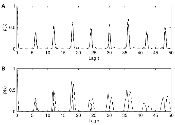
Figure 37: Recurrence probability $p(\tau)$ for two mutually coupled Rössler systems, Eqs. (• ‣ A) and (• ‣ A), for $a=0.16$, $b=0.1$, $c=8.5$, in (A) phase synchronised and (B) non-phase synchronised regime. Solid line: oscillator $\vec{x}$, dashed line: oscillator $\vec{y}$.

It is important to emphasise that the heights of the local maxima are in general different for both systems if they are only in PS and not in GS, as we will see later. But the positions of the local maxima of $p(\tau)$ coincide, and the correlation coefficient is $CPR=0.998$. For $\mu=0.02$ the systems are not in PS and the positions of the maxima of $p(\tau)$ do not coincide anymore (Fig. 37B), clearly indicating that the frequencies are not locked. In this case, the correlation coefficient is $CPR=0.115$.

It is important to emphasise that this method is highly efficient even for non-phase coherent oscillators, such as two mutually coupled Rössler systems in the funnel regime, Eqs. (• ‣ A) and (• ‣ A), for $a=0.2925$, $b=0.1$, $c=8.5$, $\nu=0.02$. We analyse again two different coupling strengths: $\mu=0.2$ and $\mu=0.05$. The peaks in $p(\tau)$ (Fig. 38) are not as well-pronounced and regular as in the coherent regime, reflecting the different time scales that play a relevant role and the broad band power spectrum of these systems. However, for $\mu=0.2$ the positions of the local maxima coincide for both oscillators (Fig. 38A), indicating PS, whereas for $\mu=0.05$ the positions of the local maxima do not coincide anymore (Fig. 38B), indicating non-PS. These results are in accordance with [150].

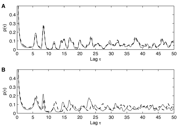
Figure 38: Recurrence probability $t(\tau)$ for two mutually coupled Rössler systems in funnel regime, Eqs. (• ‣ A) and (• ‣ A), for $a=0.2925$, $b=0.1$, $c=8.5$. (A) $\mu=0.2$ (PS) and (B) $\mu=0.05$ (non-PS). Solid line: oscillator $\vec{x}$, dashed line: oscillator $\vec{y}$.

In the PS case of this latter example, the correlation coefficient is $CPR=0.988$, and in the non-PS case, $CPR=0.145$. Note that the positions of the first peaks in $p(\tau)$ coincide (Fig. 38B), although the oscillators are not in PS. This is due to the small frequency mismatch ($2\nu=0.04$). However, by means of the index $CPR$ we can distinguish rather well between both regimes.

Furthermore, the index $CPR$ is able to detect PS even in time series which are strongly corrupted by noise [151]. Additionally, $CPR$ indicates clearly the onset of PS. In [151], the results obtained for $CPR$ in dependence on the coupling strength were compared with the Lyapunov exponents, as they theoretically indicate the onset of PS (in the phase-coherent case). The results obtained with $CPR$ coincide with the ones obtained by means of the Lyapunov exponents.

The results obtained with $CPR$ are very robust with respect to the choice of the threshold $\varepsilon$. Simulations show that the outcomes are almost independent of the choice of $\varepsilon$ corresponding to a percentage of black points in the RP between $1\%$ and $90\%$, even for non-coherent oscillators. The patterns obtained in the RP of course depend on the choice of $\varepsilon$. But choosing $\varepsilon$ for both interacting oscillators in such a way that the percentage of black points in both RPs is the same, the relationship between their respective recurrence structures does not change for a broad range of values of $\varepsilon$.

3.8.4 Detection of GS by means of recurrences

Now we demonstrate that it is also possible to detect generalised synchronisation (GS) by means of RPs [151]. When the equations of the system are known, GS can be characterised by the conditional stability of the driven chaotic oscillator [152]. However, when analysing measured time series, the model equations are usually not known. Hence, several methods based on the technique of delay embedding and on conditional neighbours have been developed to characterise GS, such as the method of mutual false nearest neighbours (MFNN) [135, 137, 153]. But systems exhibiting non-invertibility or wrinkling hamper the detection of GS by such techniques [154]. Further techniques, such as the $\delta^{p}$ and $\delta^{p,q}$ method, have been developed to overcome these problems [155].

We develop an index for GS based on RPs which can also deal with such problems. It is based on the results presented in Subsec. 3.9: the recurrence matrix of a system contains the whole information necessary to reconstruct it topologically, i. e. the recurrence matrix contains all “essential” dynamical information about the system. On the other hand, two systems connected by a homeomorphism are said to be topologically equivalent. Hence, two such systems should have a very similar recurrence matrix.

Let us consider the average probability of recurrence over time for systems $\vec{x}$ and $\vec{y}$, i. e. the recurrence rate, Eq. (41), $RR^{\vec{x}}$ and $RR^{\vec{y}}$. The average probability of joint recurrence over time is then given by $RR^{\vec{x},\vec{y}}$, which is the recurrence rate of the JRP of systems $\vec{x}$ and $\vec{y}$ [147]. If both systems are independent, the average probability of the joint recurrence will be $RR^{\vec{x},\vec{y}}=RR^{\vec{x}}RR^{\vec{y}}$. On the other hand, for both systems in GS, we expect approximately the same recurrences, and hence $RR^{\vec{x},\vec{y}}\approx RR^{\vec{x}}=RR^{\vec{y}}.$ For the computation of the recurrence matrices in the case of essentially different systems that undergo GS, it is more appropriate to use a fixed amount of nearest neighbours $N_{\text{n}}$ for each column in the matrix than using a fixed threshold (FAN, cf. Subsec. 3.2.5) [153], which corresponds, as already stated, to the original definition of RPs by Eckmann et al. [2]. $RR^{\vec{x}}$ and $RR^{\vec{y}}$ are then equal and fixed by $N_{\text{n}}$, because of Eq. (44) $RR^{\vec{x}}=RR^{\vec{y}}=N_{\text{n}}/N$. Now we call $RR=N_{\text{n}}/N$ and define the coefficient

$$S=\frac{RR^{\vec{x},\vec{y}}}{RR}$$

as an index for GS that varies from $RR$ (independent) to $1$ (GS). Furthermore, in order to be able to detect also lag synchronisation (LS) [99] with this index, a time lag is included by using the time delayed JRP, Eq. (40),

$$S(\tau)=\frac{\frac{1}{N^{2}}\sum_{i,j}^{N}\mathbf{JR}^{\vec{x},\vec{y}}_{i,j}(\tau)}{RR},$$ (113)

where $JRP$ is computed by using FAN. Then, we introduce an index for GS based on the average joint probability of recurrence $JPR$ by choosing the maximum value of $S(\tau)$ and normalising it,

$$JPR=\max\limits_{\tau}\frac{S(\tau)-RR}{1-RR}.$$ (114)

The index $JPR$ ranges from $0$ to $1$. $RR$ is a free parameter. However, simulations show that the $JPR$ index is rather independent of the choice of $RR$.

Example: Detection of GS in a driven Lorenz system

To illustrate the application of $JPR$, we analyse an interaction of two rather different chaotic oscillators, the Lorenz system (Eqs. (• ‣ A) with $\sigma=10$, $r=28$ and $b=\frac{8}{3}$) driven by a Rössler system (Eqs. (• ‣ A) with $a=0.45$, $b=2$ and $c=4$). Since the driven Lorenz system is asymptotically stable [152], the systems (• ‣ A) and (• ‣ A) are in GS. However, the shapes of both attractors in phase space are very different (Fig. 39A, B), and both are neither in LS nor in CS (Fig. 39C).

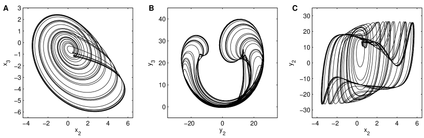
Figure 39: Projection of the (A) Rössler driving system, (B) the driven Lorenz system and (C) the plot of the second components of these systems $x_{2}$ vs. $y_{2}$.

To mimic typical experimental situations, we perform the analysis with just one component of each system. $10,000$ data points are used with a sampling time interval of $0.02$. Using $x_{3}$ and $y_{3}$ as observables, we reconstruct the phase space vectors using delay coordinates, Eq. (9), for $\vec{x}$: $m=3$, $\tau=85$ and for $\vec{y}$: $m=3$, $\tau=10$.

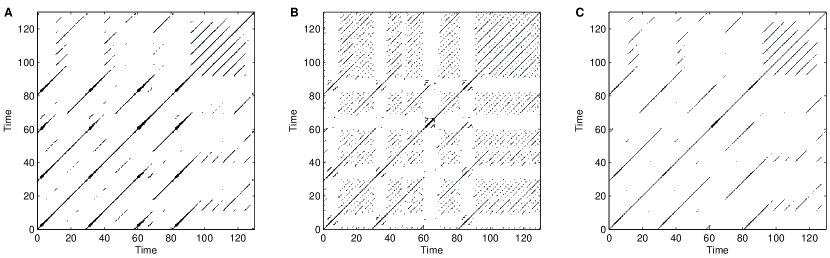
Figure 40: RPs of (A) the Rössler sub-system, (B) the driven Lorenz sub-system, and (C) the JRP of the whole system.

The RPs of both sub-systems $\vec{x}$ and $\vec{y}$ are rather similar despite of the essential difference between the shapes of the attractors (Fig. 40A, B). Therefore, the structures of each single RP are also reflected in the JRP (Fig. 40C) and consequently, its recurrence rate is rather high. With the choice $RR=0.02$ the JPR index is $JPR=0.64$ (the value of $JPR$ is similar for other choices of $RR$).

In contrast, the RPs of the independent systems ($u=y_{1}$ in Eqs. (• ‣ A), Fig. 41) look rather different (Fig. 42A and B; using embedding parameters $m=3$ and $\tau=5$ for both systems, and $RR=0.02$). Therefore, the JRP is almost empty (Fig. 42C), i. e. the mean probability over time for a joint recurrence is very small. In this case, the JRP index is $JPR=0.03$.

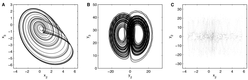
Figure 41: Projection of the (A) Rössler system, (B) the independent Lorenz system and (C) the plot of the second components of these systems $x_{2}$ vs. $y_{2}$.

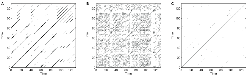
Figure 42: RPs of (A) the Rössler sub-system, (B) the independent Lorenz sub-system, and (C) the JRP of the whole system.

3.8.5 Comparison with other methods

As mentioned at the beginning of this section, there are several methods to detect GS. They might be divided in three main kinds: the conditional stability approach [152], the auxiliary system approach [156] and the mutual false nearest neighbours (MFNN) based approach [135, 137, 153].

In the case of the analysis of experimental time series, the conditional stability approach has the disadvantage that it requires the estimation of the Lyapunov exponents, which might be rather difficult by dealing with observed data. The auxiliary system approach requires an identical copy of the response system, which might be problematic to obtain in the case of measured data due to noise influences and inaccuracy in the parameters of the system. In contrast, the false nearest neighbours approach is more appropriate for the analysis of experimental data. However, if the systems to be analysed have more than one predominant time scale, some errors might occur. For example, if the systems have a slow and a fast time scale, even though the driver and the response systems are not in GS, the parameter MFNN might be of the order of one. This is because the distance between the nearest neighbours of points of the trajectory belonging to the fast time scale is of the order of the size of the attractor. For example, in the case of experimental data from electrochemical oscillators which are characterised by a non-phase coherent dynamics, the method of the false nearest neighbours does not work to detect GS. In contrast, the recurrence based method detects the onset of GS correctly (cf. Sec. 4.7). Note that the recurrence based method does not consider the distances between nearest neighbours to detect GS, but marginal and joint probabilities of recurrence for the driver and response systems. The recurrence based approach is close to the concept of transfer entropy [157] used for the detection of the direction of the coupling between systems.

Furthermore, there might be complications in the dynamics of the systems, such as non-invertibility and wrinkling, which hamper the detection of GS [154]. Some approaches, such as the time series based implementation of the auxiliary systems approach [158] and the $\delta^{p,q}$ method [155] have been introduced to overcome such problems. The $\delta^{p,q}$ method considers two points of the trajectory as neighbours, if they are neighbouring not only at one time instant, but during some longer interval of time. By means of this extension, it is possible to detect GS also in the complicated cases of non-invertibility and wrinkling. Introducing an analogous extension in the recurrence based approach, which can be accomplished increasing the embedding dimension, it is also possible to detect GS in such more intricated cases.

With respect to the computational demand, the recurrence based approach is comparable to the false nearest neighbour or $\delta^{p,q}$ approaches, as in all cases the distances between all pairs of points of the trajectories have to be computed, which is a $N^{2}$ problem.

3.8.6 Onset of different kinds of synchronisation

We have seen that the indices $CPR$ and $JPR$ clearly distinguish between oscillators in PS and oscillators which are not in PS, respectively GS. On the other hand, the synchronisation indices should not only distinguish between synchronized and not synchronised regimes, but also indicate clearly the onset of PS, respectively of GS.

In order to demonstrate that the recurrence based indices fulfill this condition, we exemplify their application with two mutually coupled Rössler systems in a phase coherent regime, Eqs. (• ‣ A), with $a=0.16$, $c=8.5$ and $\nu=0.02$. We increase the coupling strength $\mu$ continuously and compute for each value of $\mu$ the indices $CPR$, and $JPR$.

For a not too large but fixed frequency mismatch between both oscillators and increasing coupling strength, the transitions to PS and LS are reflected in the Lyapunov spectrum [133, 134]. If both oscillators are not in PS, there are two zero Lyapunov exponents, that correspond to the (almost) independent phases. Increasing the coupling strength, the fourth Lyapunov exponent $\lambda_{4}$ becomes negative (Fig. 43A), indicating the onset of PS. For higher coupling strengths, the second Lyapunov exponent $\lambda_{2}$ crosses zero, which indicates the establishment of a strong correlation between the amplitudes (Fig. 43A). This last transition occurs almost simultaneously with the onset of LS [99]. Therefore, $\lambda_{2}$ and $\lambda_{4}$ are considered in order to validate the results obtained with $CPR$ and $JPR$.

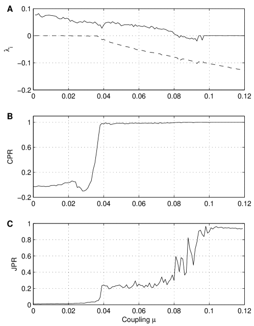
Figure 43: (A) $\lambda_{2}$ (solid line) and $\lambda_{4}$ (dashed line) as well as (B) $CPR$ and (C) $JPR$ indices in dependence of the coupling strength for two mutually coupled Rössler systems in the phase coherent regime.

Using the $CPR$ index, the transition to PS is detected when this index becomes of the order of one (Fig. 43B). The transition to PS occurs at approximately $\mu=0.037$, in accordance with the transition of the fourth Lyapunov exponent $\lambda_{4}$ to negative values. The $JPR$ index also exhibits the transition to PS, although it is an index for GS and LS. This index shows three plateaus in dependence on the coupling strength (Fig. 43C), indicating the onset of PS at the beginning of the second one. On the other hand, $JPR$ clearly indicates the onset of LS, because it becomes nearly one (third plateau) at approximately $\mu=0.1$ (Fig. 43C), after the transition from hyper-chaos to chaos, which takes place at approximately $\mu=0.08$ (Fig. 43A). Between $\mu=0.08$ and $\mu=0.1$, the values of $JPR$ have large fluctuations. This reflects the intermittent lag synchronisation [99, 159], where LS is interrupted by intermittent bursts of no synchronisation.

3.9 Information contained in RPs

In the preceding sections it has been shown that the recurrence matrix contains relevant information about the dynamics of the system under consideration. Quantifying the structures in the RP, chaos-period and even chaos-chaos transitions can be detected. Furthermore, it has been demonstrated that dynamical invariants, such as the correlation entropy, correlation dimension and mutual information can be estimated by means of RPs. On the one hand, all relevant dynamical information is fully preserved in the distance matrix $\mathbf{D}_{i,j}=\|\vec{x}_{i}-\vec{x}_{j}\|$ [160]. But on the other hand, the possibility to estimate dynamical invariants suggests that the RP contains much information about the underlying system, even though the trajectory is reduced to a matrix of zeros and ones. We next show that under some general conditions, it is possible to reconstruct the underlying attractor from the binary RP, at least topologically [161]. This is based on the fundamental property that from the RP of a scalar time series $\{x_{i}\}_{i=1}^{N}$, a new time series $\{x^{\prime}_{i}\}_{i=1}^{N}$ can be obtained, which has the same rank order as the original one. Then, from this $\{x^{\prime}_{i}\}_{i=1}^{N}$ we can reconstruct the attractor by, e. g., time delay embedding, Eq. (9). The so reconstructed manifold is topologically equivalent to the original one, i. e. there exists a homeomorphism between both attractors. However, $\varepsilon$ must be chosen appropriately to make this reconstruction possible.

The reconstruction algorithm uses the RP as input and yields the rank order $\{r_{i}\}_{i=1}^{N}$ of the underlying time series $\{x_{i}\}_{i=1}^{N}$, i. e. $x_{r_{1}}\leq x_{r_{2}}\leq\ldots\leq x_{r_{N}}$ as its output. The algorithm is based on the idea that two consecutive points $x_{r_{i}}$ and $x_{r_{i+1}}$ of this rank ordered time series can be supposed to have rather similar neighbourhoods $\mathcal{R}_{r_{i}}$ and $\mathcal{R}_{r_{i+1}}$ (cf. Eq. (85) and Fig. 44; $\mathcal{R}_{i}$ corresponds to the recurrence points in the column $i$ of the RP). Hence, the algorithm searches for columns in the RP which are “as similar as possible”, reconstructing iteratively the rank order of the time series.

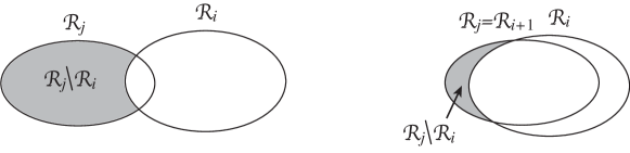
Figure 44: The rank order of a time series can be reconstructed from an RP by an algorithm which searches for the minimum $\mathcal{R}_{j}\setminus\mathcal{R}_{i}$, i. e. the set of neighbours of $x_{j}$ which are not neighbours of $x_{i}$. If $j=\min_{k}\{\mathcal{R}_{k}\setminus\mathcal{R}_{i}\}$, then $i=r_{k}$ and $j=r_{k+1}$ or vice versa, i. e. $i$ and $j$ are consecutive points in the rank ordered time series.

It is important to note that the reconstruction algorithm assumes that the maximum distance between two consecutive points in the rank ordered time series is smaller than $\varepsilon$. The reconstruction algorithm consists of three main phases and a total of nine steps which are described in detail in Appendix B.2.

To illustrate this reconstruction, we consider the Rössler attractor, Eqs. (• ‣ A), for $a=0.15$, $b=0.2$ and $c=10$. We compute the RP of the $x$-component and use it as input for the reconstruction algorithm. Then, we obtain the time series $x^{\prime}$, which has the same rank order as $x$. The both attractors derived from the delay embedded $x$ and $x^{\prime}$ are rather similar (Fig. 45). It is obvious that both attractors are homeomorphic.

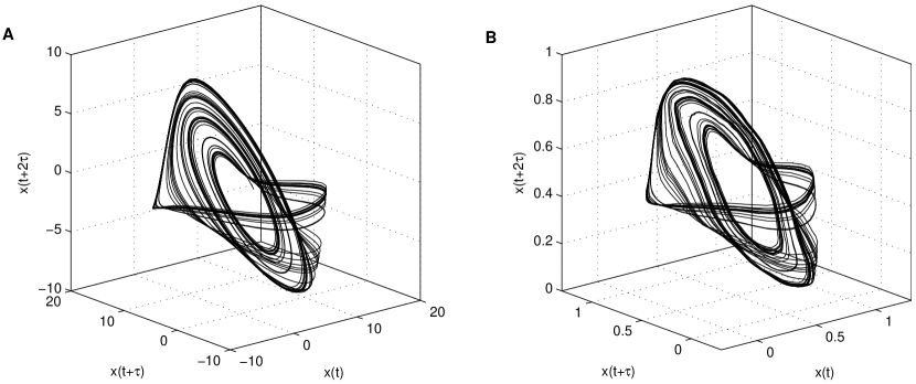
Figure 45: Embedded Rössler attractor based on the $x$-component of the original data (A) and from the reconstructed $x$-component (B) [161].

The needed number of points for the reconstruction for a given threshold $\varepsilon$ can be estimated, assuming that the values are uniformly distributed. The distance $D$ between two neighbouring points in the interval $[x_{\min},x_{\max}]$ is then exponentially distributed

$$P(D)=N\,e^{-N\,D},$$ (115)

where $N$ is the length of the time series. Assuming, without loss of generality, that $[x_{\min},x_{\max}]=[0,1]$, there are $N+1$ intervals, which have to be all smaller than $\varepsilon$. The probability that the maximal distance between two consecutive points in the interval is smaller than $\varepsilon$ is given by

$$p(\varepsilon)=\left(1-e^{-N\,\varepsilon}\right)^{N+1}.$$ (116)

Using relation (116), the minimal length of the time series necessary to reconstruct (with a probability of about 0.999) the time series (and the attractor) from an RP can be estimated. Using $\varepsilon=0.1$, only about 90 points are needed to reconstruct the time series. In general, the larger $\varepsilon$, the less points are needed to reconstruct the time series. However, if $\varepsilon$ is too large, the reconstruction algorithm works but cannot distinguish properly different points and possibly important fine structures of the system. This problem can be exemplified by choosing $\varepsilon=1/2+\delta$ in the case of the time series, which is uniformly distributed in the unit interval. Then, all points in the the band $[1/2-\delta,1/2+\delta]$ have the same neighbourhoods and hence cannot be distinguished.

Note that the reconstruction algorithm is only valid if we have the RP of a scalar time series, i. e. the reconstruction algorithm does not work for RPs of an $m$-dimensional trajectory with $m>1$. It is still an open question, whether it is possible to reconstruct the attractor from the RP of a higher dimensional trajectory. First results indicate that (under some conditions) it is possible.

3.10 Recurrence based surrogates to test for synchronisation

In Subsec. 3.8 we have considered the problems concerning the phase synchronisation analysis of complex systems when there is more than one narrowband time scale, i. e. when their power spectra are rather broad. As it was shown, RPs help to overcome this problem, allowing to extend the concept of phase synchronisation to rather complex systems.

Another important problem in the framework of synchronisation analysis is that even though the synchronisation measures may be normalised, experimental time series often yield values of these measures which are neither close to 0 nor to 1 but intermediate, e. g., 0.4 or 0.6 and hence are difficult to interpret. This problem can be overcome if the coupling strength between the interacting systems can be varied systematically and a rather large change in the measure can be observed, i. e. if it is an active experiment [133]. However, much more typical are passive experiments, in which it is not possible to change the coupling strength systematically, e. g., the possible synchronisation of the heart beats of a mother with those of her foetus [162]. In some cases, this problem has been tackled by interchanging the pairs of oscillators, i. e. testing the same foetus with a different (surrogate) mother, and using them as natural surrogates. These surrogates are independent and hence cannot be in phase synchronisation (PS) with the original system. Thus, if the synchronisation index, as Eq. (112), obtained from the original data is not significantly higher than the index obtained from the natural surrogates, there is not sufficient evidence to claim synchronisation. But even this natural surrogates approach via time series has some drawbacks. The natural variability and also the frequency of the natural surrogates are in general different from the original ones. Furthermore, the data acquisition can be expensive and at least in many cases problematic or even impossible (e. g. in the climatological interaction between the El Niño/Southern Oscillation and the North Atlantic Oscillation). In such cases it would be convenient to perform a hypothesis test based on surrogates generated by a mathematical algorithm. The null hypothesis, which the surrogates must be consistent with, is that they are independent realisations of the same underlying system, i. e. trajectories of the same underlying system starting at different initial conditions. In this section, we present a technique for the generation of surrogates, which is based on RPs. These surrogates mimic the dynamical behaviour of the system and are consistent with the null hypothesis mentioned above. Then, computing the synchronisation index between one sub-system of the original system and another sub-system of the surrogate, and comparing it with the synchronisation index obtained for the original system, we can test if an independent process can give the same index of PS.

As suggested in Subsec. 3.9, it is possible to reconstruct topologically the attractor of the system from its RP. Therefore, the RP contains all topological information about the underlying attractor. Hence, a first idea for the generation of surrogates is to change the structures in an RP consistently with the ones produced by the underlying dynamical system (the structures in the RP are linked to dynamical invariants of the underlying system, such as the correlation entropy and the correlation dimension, Subsec. 3.6) and then reconstruct the trajectory from the modified RP. Furthermore, we use the fact that there are identical columns in an RP, i. e. $R_{i,k}=R_{j,k}\ \forall k$. Thus, there are points which are not only neighbours (i. e. $\|\vec{x}_{i}-\vec{x}_{j}\|<\varepsilon$), but which also share the same neighbourhood. These points are called twins. Twins are special points of the time series as they are indistinguishable considering their neighbourhoods, but in general different and, hence, have different pasts and – more important – different futures. The key idea of how to introduce the randomness needed for the generation of surrogates of a deterministic system is that we can jump randomly to one of the possible futures of the existing twins. The generation of a twin surrogate trajectory $\{\vec{x}^{s}_{i}\}_{i=1}^{N}$ of $\{\vec{x}_{i}\}_{i=1}^{N}$ is described in detail in the Appendix B.3.

This RP based algorithm creates twin surrogates (TS) which are shadows of a (typical) trajectory of the system [163]. In the limit of an infinitely long trajectory, its TS are characterised by the same dynamical invariants and the same attractor. However, if the measure of the attractor can be estimated from the observed finite trajectory reasonably well, its surrogates share the same statistics. The trajectories of the TS are visually indistinguishable from the original ones (Fig. 46). Also their power spectra and correlation functions are consistent with the ones of the original system.

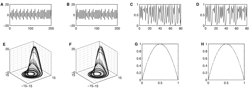
Figure 46: Segment of the $x$-component of the (A) original Rössler system, Eqs. (• ‣ A), for $a=0.15$, $b=0.2$ and $c=10$ and (B) of one twin surrogate (TS) of the Rössler system. Trajectory of the (C) Rössler system in phase space and (D) of one TS of the Rössler system. Segment of the trajectory of the (E) logistic map, Eq. (127), for $a=4.0$ and (F) of one TS of the logistic map. Phase portrait (G) of the logistic map and (H) of one TS of the logistic map (modified after [163]).

The idea behind TS to test for synchronisation consists in exchanging one original sub-system with one twin surrogate. Then, if the synchronisation index obtained for the original system is not significantly different from the one computed for the exchanged sub-systems, we have not sufficient evidence to claim synchronisation.

Suppose that we have two coupled self-sustained oscillators $\vec{x}_{i}$ and $\vec{y}_{i}$. Then, we generate $M$ pairs of TS of the joint system, i. e. $\{\vec{x}_{i}^{s_{j}}\}_{j=1}^{M}$ and $\{\vec{y}_{i}^{s_{j}}\}_{j=1}^{M}$ (for $i=1,\ldots,N$). These surrogates correspond to independent copies of the joint system, i. e. trajectories of the whole system beginning at different initial conditions. Note, that the coupling between $\vec{x}_{i}$ and $\vec{y}_{i}$ is also mimicked by the surrogates. Next, we compute the differences between the phases of the original system $\Delta\Phi_{i}=|\Phi_{x_{i}}-\Phi_{y_{i}}|$ applying, e. g., the analytical signal approach [133] and compare them with $\Delta\Phi^{s_{j}}_{i}=|\Phi_{x_{i}}-\Phi_{y_{i}}^{s_{j}}|$. Then, if $\Delta\Phi_{i}$ does not differ significantly from $\Delta\Phi^{s_{j}}_{i}$ with respect to some index for PS, the null hypothesis cannot be rejected and, thus, there is not enough evidence for PS.

Example: Statistical test of the synchronisation analysis of Rössler oscillators

We illustrate the TS technique to test for PS by considering two non-identical, mutually coupled Rössler oscillators, Eqs. (• ‣ A) and (• ‣ A), with $a=0.15$, $b=0.20$, $c=10$ and $\nu=0.015$. In this active experiment, the coupling strength $\mu$ is varied from 0 to 0.08, and a PS index for the original trajectory is calculated for each value of $\mu$. Next, we generate 200 TS and compute the PS index between the measured first oscillator and the surrogates of the second one. As PS index we use the mean resultant length $R$ of complex phase vectors [164], which is motivated by Kuramoto’s order parameter [165]

$$R=\left|\frac{1}{N}\sum\limits_{i=1}^{N}e^{j\Delta\Phi_{i}}\right|.$$ (117)

$R$ takes values in the interval from 0 (non PS) to 1 (perfect PS) [164]. Let $R^{s_{i}}$ denote the PS index between the first oscillator and the surrogate $i$ of the second one. To reject the null hypothesis at a significance value $\alpha$, $R$ must be larger than $(1-\alpha)\cdot 100$% of all $R^{s_{j}}$. This corresponds to computing the significance level from the cumultative histogram at the $(1-\alpha)$ level.

For $\mu<0.025$, $R$ of the original system is, as expected, below the significance level (Fig. 47A) and, hence, the difference is negative (Fig. 47B). For higher values of $\mu$, $R$ exceeds the significance level (the difference becomes positive). This is in agreement with the criterion for PS via Lyapunov exponents $\lambda_{i}$ [133]: $\lambda_{4}$ becomes negative at $\mu\approx 0.028$ (Fig. 47C), which approximately coincides with the intersection of the curve of $R$ for the original system and the significance level (zero-crossing of the curves in Fig. 47B). Therefore, the PS region can be successfully recognised by means of the TS.

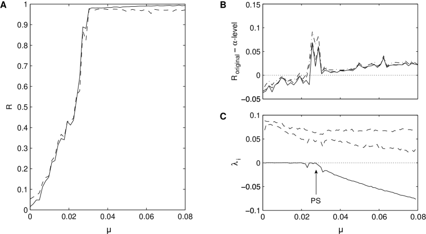
Figure 47: (A) Mean resultant length $R$ of the original two mutually coupled Rössler systems, Eqs. (• ‣ A) and (• ‣ A), with $a=0.15$, $b=0.20$, $c=10$, a frequency mismatch of $\nu=0.015$ (solid), and significance level of 1% (dashed). (B) Difference between $R$ of the original data and significance level of 1% (solid), 2% (dashed) and 5% (dashed-dotted). (C) The four largest Lyapunov exponents for the considered 6-dimensional system. $\lambda_{4}$ is highlighted (solid) and the arrow indicates the transition to PS.

Note that also the significance limit increases when the transition to PS occurs (Fig. 47A). As the TS mimic both the linear and nonlinear characteristics of the system, the surrogates of the second oscillator have the same mean frequency in the PS region as the first original oscillator. Therefore, $R^{s_{j}}$ is rather high (it can take on values of up to $0.97$). However, $\Phi_{x_{i}}$ and $\Phi_{y_{i}}^{s_{j}}$ do not adapt to each other as they are independent, thus, the value of $R$ for the original system is significantly higher than the $R^{s_{j}}$ and, hence, it indicates PS. We notice that even though the obtained value for a normalised PS index is higher than 0.97 (right side of Fig. 47A), this still does not provide conclusive evidence for PS. The knowledge of the PS index alone is not sufficient to infer PS. Especially in passive experiments, the synchronisation analysis should always be accompanied by a hypothesis test.

3.11 Localisation of unstable periodic orbits by RPs

The localisation and quantification of unstable periodic orbits (UPOs) in chaotic attractors is very important as an orbit on a chaotic attractor is the closure of the set of UPOs which build the skeleton of the attractor. Roughly speaking, a trajectory, therefore, can be regarded as jumping from one UPO to the next one. Furthermore, the set of UPOs in an attractor is a dynamical invariant of the system [166], as mentioned in Sec. 2.

RPs can be used to easily localise UPOs in chaotic time series [69, 48, 167]. The main idea is the following: when the trajectory of the system comes close to an UPO, it stays in its vicinity for a certain time interval, whose length depends on how unstable the UPO is. This is reflected in the RP, as the pattern corresponding to periodic movement consists of uninterrupted equally spaced diagonal lines (if we consider the RP of the original trajectory in phase space and not a projection). Hence, UPOs present in the underlying system can be localised by identifying such “windows” inside the RP, where the patterns correspond to a periodic movement.

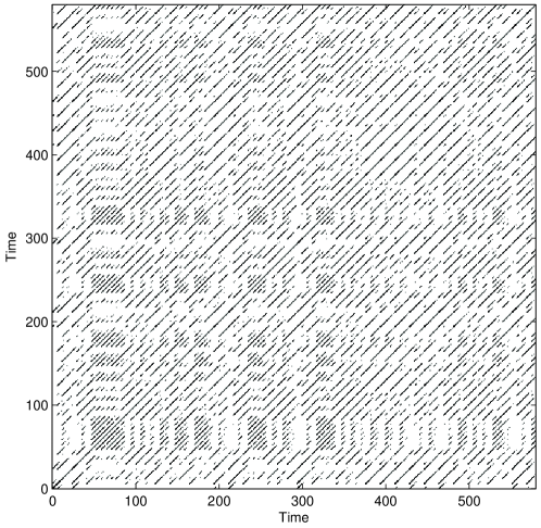
Figure 48: RP of the Rössler system, Eqs. (• ‣ A), with $a=0.15$, $b=0.2$ and $c=10$. The three components $x$, $y$, and $z$ were used for the computation, as well as the $L_{\infty}$-norm.

For example, we can consider the Rössler system, Eq. (• ‣ A), with $a=0.15$, $b=0.2$ and $c=10$. In its RP, many of such “periodic” windows can be identified (Fig. 48). Moreover, the distance between the diagonal lines can vary from window to window, indicating a different UPO with a different period. The period can be estimated by the vertical distances between the recurrence points (e. g. by $\langle T^{(2)}\rangle$ or the mean length of the white vertical lines) in the periodic window multiplied by the sampling time of the integrated trajectory. The UPO, which the trajectory of the Rössler system is close to, can easily be identified in the magnifications of three different windows of the RP as well as from the corresponding segments of the trajectory (Fig. 49).

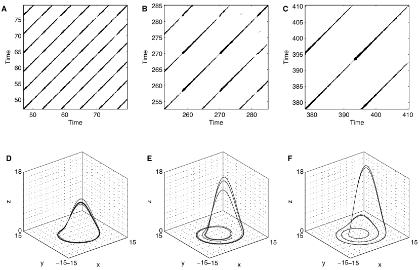
Figure 49: (A–C) Magnifications of different periodic windows of the RP presented in Fig. 48, and (D–F) the corresponding segments of the trajectory. The trajectories reveal the UPOs of period 1 (D), period 2 (E) and period 3 (F).

The problem of using this method to localise UPOs is that a finite-length trajectory cannot visit all UPOs embedded in the attractor. Hence, it is still an open problem how to localise all of them using RPs. However, first results indicate that there might be ways to overcome this difficulty. Furthermore, the authors in [167] claim that RPs are not appropriate to find UPOs of high periods or UPOs which are very unstable. Nevertheless, the other existing methods to detect UPOs based on time series have the same problem [168].

3.12 Influence of noise on RPs

In this section, an estimation of the errors due to observational noise on the quantification of RPs is derived. Based on this estimation it is possible to give a criterion to choose an optimal threshold $\varepsilon$ to minimise these errors [52].

Assume that we have a given scalar time series $x_{i}$ corrupted by observational independent Gaussian noise $\xi_{i}$, i. e. we have measured $y_{i}=x_{i}+\xi_{i}$. Then, in the simplest case of non-embedding, the recurrence matrix, Eq. (10), becomes

$$\mathbf{\tilde{R}}_{i,j}=\Theta\left(\varepsilon-\left|x_{i}-x_{j}+\xi_{i}-\xi_{j}\right|\right).$$ (118)

In order to estimate how the observational noise changes the structures in $\mathbf{\tilde{R}}_{i,j}$ with respect to $\mathbf{R}_{i,j}$, we consider the probability $\mathbf{P}_{i,j}$ to find a recurrence point at the coordinates $(i,j)$.

For an ensemble of realisations of the noise $\mathcal{W}(0,\sigma^{2})$, the observation $y_{i}$ is Gaussian distributed with mean $x_{i}$ and standard deviation $\sigma$. Furthermore, we assume without loss of generality that $x_{i}=0$ and $x_{j}=-\mathbf{D}_{i,j}$ (cf. Eq.(26)). Then the probability to find a recurrence point at the coordinates $i,j$ is given by

$$\mathbf{P}_{i,j} = \left(\frac{1}{\sqrt{2\pi}\sigma}\right)^{2}\int\limits_{-\infty}^{\infty}e^{-\frac{\xi_{i}^{2}}{2\sigma^{2}}}\int\limits_{\xi_{i}-\varepsilon}^{\xi_{i}+\varepsilon}e^{-\frac{(\xi_{j}-\mathbf{D}_{i,j})^{2}}{2\sigma^{2}}}d\xi_{j}\;d\xi_{i}$$ (119)

$$= \frac{1}{8}\Bigg{\{}\mathrm{erfc}^{2}\left(\frac{\mathbf{D}_{i,j}-\varepsilon}{2\sigma}\right)-\mathrm{erfc}^{2}\left(-\frac{\mathbf{D}_{i,j}-\varepsilon}{2\sigma}\right)+\mathrm{erfc}^{2}\left(-\frac{\mathbf{D}_{i,j}+\varepsilon}{2\sigma}\right)-$$

$$\quad\mathrm{erfc}^{2}\left(\frac{\mathbf{D}_{i,j}+\varepsilon}{2\sigma}\right)\Bigg{\}}$$

where $\text{erfc}(\cdot)=1-\text{erf}(\cdot)$. Eq. (119) maps the distance matrix $\mathbf{D}_{i,j}$ to the probability matrix $\mathbf{P}_{i,j}$ to find a recurrence point in the RP of $y_{i}=x_{i}+\xi_{i}$ at the coordinates $(i,j)$ for a fixed underlying process and an ensemble of realisations of the observational noise. The smaller the values of $\sigma$ the closer $\mathbf{P}$ comes to a Heaviside function (Fig. 50). In the presence of noise, recurrence points of the underlying system $x_{i}$ are recognised as such with probability less than one, and analogously for non-recurrence points.

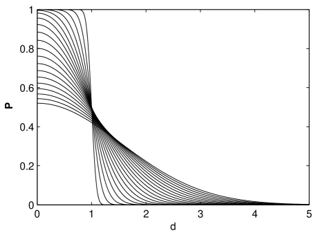
Figure 50: Dependence of $\mathbf{P}$ on $d=\mathbf{D}/\sigma$ for different $\sigma\in[0.05\varepsilon\ \varepsilon]$ in steps of $0.05\varepsilon]$ [52].

Already a small amount of noise reduces the reliability of the quantification of RPs, e. g. for a noise level of $4\%$ the probability that $\left|y_{i}-y_{j}\right|<\varepsilon$ for $\left|x_{i}-x_{j}\right|\approx\varepsilon$ is reduced from one to less than $0.6$, i. e. more than $40\%$ of the recurrence points are not recognised.

If the density $\varrho$ of the differences $x_{i}-x_{j}$ is given, the percentage of recurrence points $p_{b}(\varepsilon,\sigma)$ that are properly recognised in the presence of observational noise can be calculated

$$p_{b}(\varepsilon,\sigma)=\frac{\int\limits_{-\varepsilon}^{\varepsilon}\mathbf{P}(\mathbf{D},\varepsilon,\sigma)\varrho(\mathbf{D})dD}{\int\limits_{-\varepsilon}^{\varepsilon}\varrho(\mathbf{D})dD}.$$ (120)

Analogously, it is possible to compute the percentage of properly recognised non-recurrence points

$$p_{w}(\varepsilon,\sigma)=\frac{\int\limits_{-\infty}^{-\varepsilon}\left(1-\mathbf{P}(\mathbf{D},\varepsilon,\sigma)\right)\varrho(\mathbf{D})dD+\int\limits_{\varepsilon}^{\infty}\left(1-\mathbf{P}(\mathbf{D},\varepsilon,\sigma)\right)\varrho(\mathbf{D})dD}{1-\int\limits_{-\varepsilon}^{\varepsilon}\varrho(\mathbf{D})dD}$$ (121)

Hence, as usually, two types of errors can be distinguished:

1. false negative: a recurrence point is not recognised as such with probability $1-p_{b}$ and

2. false positive: a non-recurrence point is recognised as a recurrence point with probability $1-p_{w}$.

In order to minimise these errors, the threshold $\varepsilon$ should be chosen in such a way that $p_{b}$ and $p_{w}$ are maximised simultaneously. Even though the results depend on the distribution of the time series, numerical simulations show that the choice of the threshold should be at least five times the standard deviation of the observational noise $\varepsilon\approx 5\sigma$. This minimal choice is appropriate for a vast class of processes (e. g. maps) [52]; higher-dimensional systems may require even a higher threshold $\varepsilon>5\sigma$. If $\varepsilon$ is smaller, effects of the observational noise will have a dominant influence on the detection of recurrence points. On the other hand, if $\varepsilon$ is near the standard deviation of the underlying process, the density of recurrence points will be too high to detect detailed structures of the underlying process.

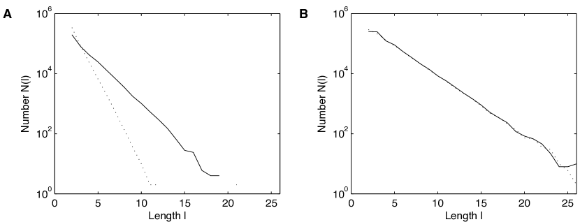
Figure 51: Cumulative distribution of diagonal lines for the logistic map, Eq. (127), for $a=4$ and 3,000 data points, using (A) the usual choice of $\varepsilon\approx\sigma$ and (B) optimal choice of $\varepsilon\approx 5\sigma$ (solid line: without noise, dashed line: with $10\%$ noise) [52].

The impact of the proper choice of the threshold can be demonstrated by studying the cumulative distribution of diagonal lines in the RP, e. g. for the logistic map, Eq. (127), contaminated with Gaussian white noise. For the choice of the threshold as the standard deviation of the observational noise, $\varepsilon=\sigma$, the distribution of the diagonal lines of the underlying process is biased when observational noise is present (Fig. 51A). In contrast, with the proper choice $\varepsilon=5\sigma$ the distribution of the diagonal lines in the presence of noise coincides with the distribution of the diagonal lines in the absence of noise (Fig. 51B).

Furthermore, noise has an influence on the estimation of the dynamical invariants. Using the knowledge about the relationship between the dynamical invariants and the noise as well as the threshold $\varepsilon$, the noise level can be estimated. Such a relationship has been developed for the correlation entropy [169], where a fit of the analytical function $K_{2}(\varepsilon)$ to the obtained entropy computed by RPs is used to estimate the noise-level $\sigma$.

4 Applications

The search for applications of RP based methods in the World Wide Web reveals numerous works (at present, the Scirus search engine finds over 1,000 different works). RPs and the RQA are most popular in physiology. However, various successful applications in other fields of life science, as neuroscience and genomics, but also in ecology, physics, chemistry, earth science and astrophysics, engineering and economy have also been published. In the following, some overview about the potentials of RPs for applications is presented by means of a few selected examples.

One of the first applications of RPs was the analysis of heart beat intervals [13]. This study has revealed typical features in RPs for cardiac transplant patients and cardiomyopathy patients who underwent volume loading. Applying the RPs, it was inferred that the dimensionality and entropy of the heart beat variations decrease during a significant cardiac event like myocardial infarction or ventricular tachycardia. The investigation of the cardiac system is one of the classical application fields of RPs and RQA. Numerous studies used, e. g., the RQA in order to monitor disease [15] or to detect predecessors of cardiac arrhythmia [14].

In further life science research RPs, OPRPs as well as RQA have been applied to, e. g., electromyography data [170], measurements based on eye movements [171], data of postural fluctuations [172], EEG data [173, 16, 17, 18, 97] or other neuronal signals [174], in order to study the interacting physiological processes. Characteristic patterns and rather fine frequency modulations in voice streams can be visualised by the means of RPs [61].

An RQA was applied to a DNA sequence of the genome Caenorhabditis elegans [175], which is a small (approximately 1 mm long) soil nematode found in temperate regions. This analysis has revealed long-range correlations in the introns and intergenic regions, which are caused by the frequent recurrence of oligonucleotides (a short sequence of some hundreds of nucleotides) in these regions. The recurrence of the oligonucleotides has been discovered by computing the recurrence rate for overlapping windows which cover the DNA sequence. Other studies confirm such long-range correlations in DNA sequences [176].

An analysis based on RPs has been used to study monopole giant resonance in atomic nuclei [177]. Due to the fact that a nucleus consists of protons and neutrons, the oscillations can be divided into two modes: (1) the densities of protons and neutrons oscillates in phase (isoscalar mode) and (2) the two densities have opposite phases (isovector mode). Both of these modes exhibit significantly different RPs. Where the oscillation of the isoscalar mode has an RP typical for regular oscillations, the RP for the isovector mode uncovers non-stationary and chaotic dynamics. Other applications in physics were performed in order to estimate the signal to noise ratio in laser systems [52], or to estimate dynamical invariants, as the dimensionality, of fluid flow systems [116].

In chemistry the RQA was applied to data from the Belousov-Zhabotinsky reaction especially to study the transitions during its chemical evolution in an unstirred batch reactor [178]. Using the RQA measures, the transitions between periodic, quasi-periodic and chaotic states could be observed. By means of JRPs, the synchronisation between electrochemical oscillators were studied [151]. Other applications in chemistry/molecular biology concern the dynamics of chemical processes, for example in molecular dynamics simulations of poly-peptides [11, 12] or to detect chaotic transitions of Nicotinamide adenine dinucleotide [179]. Applying the RQA to glycoproteins of a virus has uncovered the interaction between specific glycoprotein partners [180].

Applications in earth science are yet rare. CRPs have been used in order to compare similar dynamical evolutions in palaeo-climate and modern rainfall data in NW Argentina [7]. The ability of CRPs to align time scales of geophysical profiles were demonstrated on rock- and palaeo-magnetic data from marine sediments [6]. The estimation of $K_{2}$ by means of RPs was used to compare a general circulation model (GCM) with re-analysis data [181]. A recent study applied RPs on geomagnetic activity data represented by several measurements (proxies for eastward and westward flowing polar currents) and derived the mutual information from these RPs [8].

An astrophysical application of RPs has used radiocarbon data of the last 7,000 years [3]. The atmospheric radiocarbon is influenced by the variation of solar activity and exhibits century-scale variations of chaotic nature. The main findings based on the RP analysis and a surrogate test reveal that these variations are indeed different from linear processes and that there are different types of large events affecting their tendency to recur (e. g. the Maunder minimum seems to be unique, whereas the Oort and Dalton minima as well as the Medieval maximum tend to recur). Moreover, the authors have found that the present-day data are similar to the Medieval maximum. Besides, RPs were also used in order to investigate the synchronisation and phase difference in annual sunspot areas [182, 5].

The stability of the orbits of terrestrial planets in the habitable zone of five extra-solar systems were investigated by computing dynamical invariants derived from RPs [4]. By using the $K_{2}$ entropy, one full stable system, three systems with planets whose orbits are stable for a long time and one unstable system were detected.

In engineering, applications of RPs or RQA are yet also rather rare. One of the first has applied RPs to time series generated by models of the Twin-T, Wien-bridge and other chaos generating electronic oscillator circuits [9]. Through visual inspection of the RPs, the chaotic behaviour of the model results has been confirmed. RPs have been used to estimate optimal embedding parameters and vicinity threshold which are used for a noise reduction scheme in human speech signals [183]. A recent work proposed the method of JRPs as a very effective diagnosis tool in order to detect damage-induced changes in materials [10].

RPs have been used for research in economics. For example, RPs have been inspected visually in order to find chaos in economics time series [184, 185]. Whereas these visual inspections could not find chaos in the considered economic time series (e. g. unemployment rate, private domestic investment, foreign exchange rate), a combined “close returns” and surrogate test seems to reveal nonlinear dependencies among data of exchange rates. Other studies of foreign exchange data have used the RQA and have also found significant correlations between various currencies, which were not obvious in the raw exchange data [186]. In contrast to the results in [185], the research of others who used the RQA has revealed chaos in exchange data [187, 188]. Other applications on stock indices tried to predict “bubble bursts” on the stock market [189]. Moreover, the attempts to predict lottery numbers by the means of recurrences should also be mentioned here, even this work seems to be not really serious (numerous sites in the WWW).

In the following subsections, we show in detail some exemplary applications of RPs, CRPs, JRPs and their quantification (RQA and dynamical invariants) to different kinds of experimental data.

4.1 RQA analysis in neuroscience

First, we illustrate the capabilities of the RQA to detect transitions in measured physiological data.

The activity of rather large ensembles of neurons (which act like nonlinear devices) is macroscopically measurable in the electroencephalogram (EEG) of the human scalp, which results from a spatial integration of post-synaptic potentials. Applying nonlinear techniques like the estimation of the correlation dimension to EEG has a long tradition (e. g. [190, 191, 192, 193, 194]). However, most techniques are only well-defined for stationary time series generated by a low dimensional dynamical system, and, hence, they fail in investigating event-related brain potentials (ERPs) because they are non-stationary by definition [195]. Event-related potentials are characteristic changes in the EEG of a subject during and shortly after a certain (e. g. visual or acoustic) stimulus (surprising moment). The notation for an ERP is, e. g., N100 or P300, where N means a negative and P a positive potential and the number corresponds to the time of ERP onset after the stimulus in milliseconds.

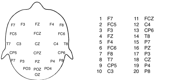
Figure 52: Localisation of the electrodes on the head.

Traditionally, ERP waveforms are determined by computing an ensemble average of a large collection of EEG trials that are stimulus time locked. By averaging the data points, which are time locked to the stimulus presentation, it is possible to filter out some signal (ERP) of the noise (spontaneous activity). This way, the P300 component of the ERP (i. e. brain activity 300 ms after the onset of the stimulus) was the first potential discovery to vary in dependence on subject internal factors, like attention and expectation, instead on physical characteristics [195]. The amplitude of the P300 component is highly sensitive to the novelty of an event and its relevance (surprising moment). So this component is assumed to reflect the updating of the environmental model of the information processing system (context updating) [196, 197]. There are two main disadvantages of the averaging method. On the one hand, the number of trials needed to reduce the signal-to-noise-ratio is rather high. This disadvantage is crucial for example in clinical studies, studies with children or studies in which repeating a task would influence the performance. On the other hand, several high frequency structures reflecting other important brain activities are filtered out by using the averaging method. It is, therefore, desirable to find new approaches for analysing event related activity on a single trial basis. Applying the concepts of the RQA to electro-physiological data could be one way of dealing with this problem.

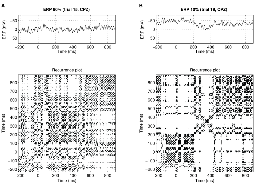
Figure 53: ERP data for event frequencies of 90% (A) and 10% (B), and their corresponding recurrence plots. For the lower event frequency (B) more clusters of recurrence points occur at 100 ms and 300 ms. Furthermore, a white band marks a transition in the process [17].

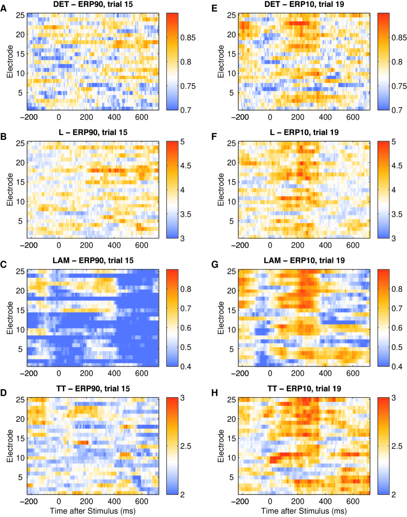
Figure 54: RQA measures for selected trials for event frequencies of 90% (A–D) and 10% (E–H). The P300 component reflects the surprising moment and can be detected in single trials by the measures $LAM$ (G) and $TT$ (H), which base on the vertical structures in the RP. The measures based on diagonal structures, $DET$ and $L$, are less apparent [17].

For this study, we analyse measurements of an Oddball experiment [17]. It studies brain potentials during a stimulus presentation; here acoustic stimuli are used. In the analysis of a set of 40 trials of ERP data for an event frequency of 90% (ERP90) and a second set of 31 trials for an event frequency of 10% (ERP10), the RQA measures $DET$ and $L$, and the vertical structures based measures $LAM$ and $TT$ are computed. The ERPs is measured at 25 electrodes (Fig. 52) with a sampling rate of 4 ms. Our aim is to study single trials in order to find transitions in the brain processes as a consequence of unexpected stimulation. Due to the N100 and the P300 components in the data, the RPs show varying structures changing in time (Fig. 53). Diagonal structures and clusters of black points occur. The non-stationarity of the data around the N100 and P300 causes extended white bands along these times in the RPs. However, the clustered black points around 300 ms occur in almost all RPs of the ERP10 data set. The application of the measures of complexity to these ERP data discriminates the single trials with a distinct P300 component resulting from a low surprise moment (high frequent events, ERP90 data) in favour of such trials with a high surprise moment (less frequent events, ERP10 data; Fig. 54). The $LAM$ is the most distinct parameter in this analysis. In the ERP data the $LAM$ reveals transitions from less to more laminar states after the occurrence of the event and a transition from more laminar states to less laminar ones after approximately 400 ms. These transitions occur inside bounded brain areas (parietal to frontal along the central axis). The comparable measures $DET$ and $LAM$ as well as $L$ and $TT$ are quite different in their amplitudes. There are also differences in time and brain location of the found transitions.

These results show that the measures based on vertical RP structures uncovers transitions, which are not found by the RQA measures based only on the diagonal RP lines. The RQA indicate transitions in the brain processes into laminar states due to the surprising moment of observed events.

4.2 RQA analysis of financial exchange rates

The study of economic systems by time series analysis is a challenging effort. Economic cycles are usually characterised by irregular variations in amplitude and period length, rising the discussion whether the economical dynamics is, e. g., stochastic or chaotic, and whether it is stationary. Several approaches from nonlinear data analysis have been applied in order to discern the type of dynamics in economic time series, like the BSD test [198] or the Kaplan’s test [199]. In the last years, RPs and their quantitative analysis have also become popular for testing for nonlinearity of economic dynamics [185, 187]. In the following example the RQA is applied to financial exchange rates in order to assess a nonlinearity in them [188].

Many open-economic theoretical models require the fulfilment of the purchasing power parity (PPP). This is an equilibrium assumption in the market for tradeable goods: a good in a country should sell for the same price as in any other country. One consequence is that the real exchange rate must be stationary. Using $P$ as the domestic price, $P^{*}$ as the foreign currency price and $S$ as the exchange rate, a formal description of this assumption is

$$P=SP^{*}.$$ (122)

The real exchange rate, i. e. the ratio of the price of the domestic to foreign goods, is

$$E=\frac{SP^{*}}{P},$$ (123)

and measures the price competitiveness. If the PPP assumption holds, this real exchange rate $E$ must be stationary. Therefore, it is important to test for stationarity of $E$. Several applied tests for stationarity are based on the assumption that the process driving the dynamics of the exchange rates is inherently linear. Hence, if the underlying process is nonlinear, these tests might erroneously reject the null-hypothesis that $E$ is a stationary process, even though it is stationary indeed. In order to assess nonlinearity in exchange rates, RQA in connection with a surrogate test can be used.

The analysed data are quarterly US Dollar based exchange rates for 16 foreign countries (Austria, Belgium, Canada, Denmark, Finland, France, Germany, Greece, Ireland, Italy, Japan, The Netherlands, Norway, Spain, Switzerland and United Kingdom) spanning the time from January 1957 to April 1998 (168 observations). First, the data are transformed with a stationary-in-mean series and then filtered in order to remove linear stochastic dependencies by fitting an AR model, Eq. (125). For details of the data aquisition and preprocessing, as well as a comprehensive explanation of all tests applied to these data, see [188].

Table 4: Used threshold $\varepsilon$ and RQA measures of exchange rates. RQA measures exceeding the 95${}^{\text{th}}$ percentiles of the empirical distribution based on surrogates (in parenthesis) are shown in bold font. $RR$ and $DET$ values are given in %.

Country	$\varepsilon$	$RR$		$DET$		$ENT$		$L_{\max}$
Austria	0.086	5.02	(2.77)	53.5	(44.7)	3.39	(2.01)	35	(26)
Belgium	0.048	4.62	(1.59)	60.6	(30.8)	2.98	(1.38)	33	(18)
Canada	0.066	5.10	(4.08)	72.9	(65.7)	3.03	(2.99)	32	(31)
Denmark	0.127	4.98	(5.91)	58.3	(84.1)	2.10	(3.59)	25	(35)
Finland	0.167	5.01	(8.33)	19.5	(79.2)	2.59	(4.25)	20	(38)
France	0.155	4.93	(3.59)	81.3	(68.3)	1.82	(2.63)	23	(25)
Germany	0.089	4.98	(3.22)	85.4	(60.6)	3.28	(2.50)	31	(26)
Greece	0.062	5.02	(4.86)	60.4	(67.6)	3.25	(3.22)	37	(36)
Ireland	0.177	5.02	(8.15)	46.4	(83.5)	1.14	(4.02)	20	(40)
Italy	4.350	4.86	(8.19)	46.0	(36.2)	2.65	(3.02)	35	(32)
Japan	0.079	5.08	(2.62)	56.7	(54.7)	3.52	(2.52)	35	(26)
The Netherlands	0.110	5.08	(3.21)	74.0	(60.8)	3.35	(2.55)	32	(28)
Norway	0.075	5.02	(2.74)	63.6	(50.6)	3.38	(2.32)	37	(25)
Spain	0.182	5.05	(5.60)	20.3	(72.7)	1.92	(3.46)	22	(31)
Switzerland	0.055	5.70	(1.33)	86.6	(24.3)	4.30	(0.05)	40	(17)
United Kingdom	0.166	5.11	(7.88)	42.4	(84.2)	0.62	(4.01)	17	(39)

The RQA measures $RR$, $DET$, $ENT$ and $L_{\max}$ (see Sec. 3.5) are calculated for each time series. The embedding parameters used are $m=20$ and $\tau=1$; the recurrence threshold $\varepsilon$ is determined such that it is the smallest value at which all RQA parameters are non-zero (Tab. 4). Then, 500 surrogate series for each currency are produced by simply shuffling the exchange data. This shuffling destroys dependencies in time but preserves the distribution of the original series. The same RQA measures are then calculated from these surrogates using the same embedding and RP parameters as for the corresponding original data series. This leads to an empirical distribution of the RQA measures under the null-hypothesis of independence in time and an identical distribution. The authors claim that if all RQA measures $RR$, $DET$, $ENT$ and $L_{\max}$ of the original data series exceed the 95${}^{\text{th}}$ percentile of the empirical distribution, the assumption of linearity must be rejected. This is indeed the case for the currencies of Austria, Belgium, Canada, Germany, Greece, Japan, The Netherlands, Norway and Switzerland (Tab. 4). The assumption of a linear stochastic process cannot be rejected for the currencies of Denmark, Finland, Ireland, Spain and United Kingdom. These findings are supported by an application of the Kaplan’s test [188].

In conclusion, the authors of [188] claim that the real exchange rates are probably driven by a nonlinear mechanism. This can help to sustain the PPP assumption even using data which pretend to be non-stationary, but analysed under linear assumptions.

4.3 Damage detection using RQA

Early damage detection of mechanical systems is a crucial task for preventing catastrophic failures or minimise maintenance costs. Vibration based structural health monitoring (SHM) is one approach for damage detection. The main idea is to look for early signatures in the dynamical response (like frequencies, phase ratios, mode shapes) of excitations (applied load) before serious problems arise. In a recent work, RQA has been employed for SHM simulation and proved to perform better than standard frequency based measures [10].

A thin plate of hot-rolled steel is used in a finite element model in order to simulate dynamic response under different damage conditions. The model contains 624 elements, representing a plate of size $0.660\times 0.408\times 3.175\ 10^{-3}$ m³, and with clamp-free boundary conditions (Fig. 55). The simulated damage is imposed as a cut in the plate with increasing length extending to 25% in increments of 5%. The strain is measured by using nine sensors, and the forcing input is applied at one node near the left corner (Fig. 55), which is excited by a chaotic vibration, obtained from the Lorenz oscillation, Eq. (• ‣ A). Detailed explanations about the basic assumptions, the model and parameters can be found in [10].

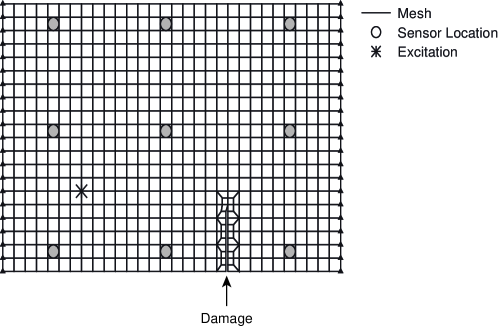
Figure 55: Schema of the plate model with sensor, load and damage locations [10].

The phase space vector is constructed by using all nine sensor measurements as components, i. e. the phase space is 9-dimensional. Next, CRPs between each damage stage and the undamaged case are computed. As the simulated damage increases, the phase space trajectory differs more and more from the trajectory of the undamaged case, what is reflected by a diminishment of the recurrence points and diagonal lines in the CRP. Therefore, the RQA measures $RR$, $DET$ and $ENTR$ are computed within sliding windows of length 10,000 (shift of 1,400 points) from the CRPs.

The measures $RR$ and $DET$ clearly identify and quantify the damage scenarios for damages larger than 10% (Fig. 56). The $ENTR$ measure is not able to detect the damage clearly (only for 25%). The sensitivity of the $RR$’s and $DET$’s changes with damage can be compared with the plate’s modal frequencies, which are often used in SHM as benchmarks for comparison to the proposed technique. Both $RR$ and $DET$ exhibit larger changes due to the damage than the first three modal frequencies $f_{1}$, $f_{2}$ and $f_{3}$ (Fig. 56). The highest changes are 33% for $RR$ and 22% for $DET$, where the highest changes for $f_{1}$, $f_{2}$ and $f_{3}$ are less than 10%.

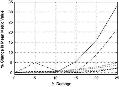
Figure 56: Change of the RQA measures with damage along with the first three modal frequencies: solid – $RR$, dashed – $DET$, dotted – $ENTR$ and dashed-gray – $f_{1}$, $f_{2}$, $f_{3}$ [10].

In conclusion, the RQA based measures appear to be a more effective tool for monitoring subtle changes in mechanical structures. Their advantage lies in a high sensitivity and simple computation. Moreover, the probabilistic nature of this method does not require assumptions about the underlying dynamics, like stationarity or linearity.

4.4 Time scale alignment of geophysical borehole data

The problem of adjustment of data series with various time scales occurs in many occasions, e. g., data preparation of tree rings or geophysical profiles. Often a large set of geophysical data series is gained at various locations (e. g. sediment cores). Therefore, these data series have different lengths and time scales. The first step in the analysis of these time series is the synchronisation of both time scales. Usually, this is done visually by comparing and correlating each maximum and minimum in both data sets by hand (“wiggle matching”), which includes the human factor of subjectiveness and is a lengthy process. The use of CRPs can make this process more objective and automatic.

CRPs contain information about the time transformation which is needed to align the time scales of two data series. This is revealed by the distorted main diagonal, the LOS (Subsecs. 3.2.3 and 3.3). A nonparametric rescaling function is provided by isolating this LOS from the CRP, which can be used for the re-alignment of the time scales of the considered time series.

4.4.1 Time scale alignment of geological profiles

Here we apply this technique to re-adjust two geological profiles (sediment cores) from the Italian lake Lago di Mezzano [200, 55]. The profiles cover approximately the same geological processes but have different time scales due to variations in the sedimentation rates at the different sites. The first profile (LMZC) has a length of about 5 m and the second one (LMZG) of about 3.5 m (Fig. 57). From both profiles a huge number of geophysical and chemical parameters were measured. Here we focus on the rock-magnetic measurements of the normalised remanent magnetisation intensity (NRM) and the susceptibility $\kappa$.

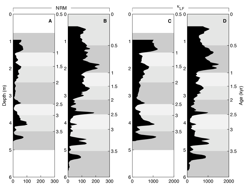
Figure 57: Rock-magnetic measurements of lake sediments with different time scales. Corresponding sections are marked with different grey values [55].

We use the time series NRM and $\kappa$ as components for the phase-space vector, resulting in a two-dimensional system. However, we apply an additional embedding using the time-delay method [201]. A rather small embedding decreases the amount of line structures representing the progress with negative time [54]. Using the embedding parameters dimension $m=3$ and delay $\tau=5$ (empirically found for these time series), the final dimension of the reconstructed system is six. The corresponding CRP reveals a partly disrupted, swollen and bowed LOS (Fig. 58). This LOS can be automatically resolved, e. g. by using the LOS-tracking algorithm as described in the Appendix B.1. The application of this LOS as the time-transfer function to the profile LMZG re-adjusts its time series to the same time scale as LMZC (Fig. 59). This method offers a helpful tool for an automatic adjustment of different geological profiles, in contrast to the rather subjective method of “wiggle matching” (adjustment by harmonising maxima and minima by eye) used so far.

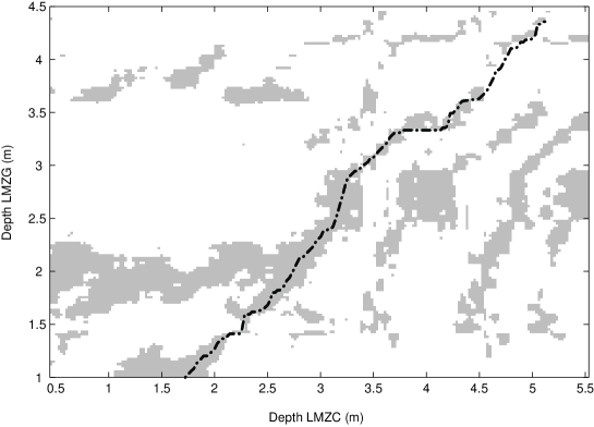
Figure 58: Cross recurrence plot between rock-magnetic data shown in Fig. 57. The dash-dotted line is the resolved LOS which can be used for re-adjustment of the time scales of both data sets [55].

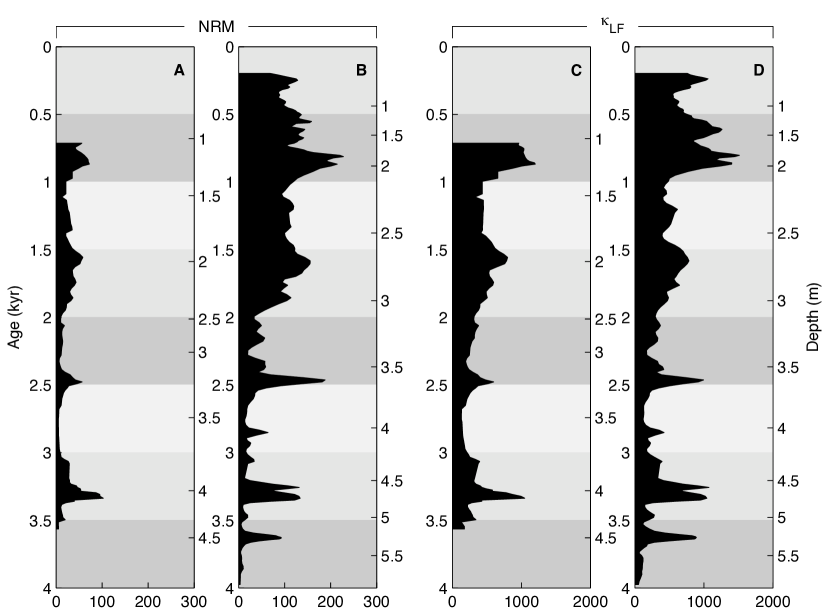
Figure 59: Geological profiles after re-adjustment using the LOS which was found with the CRP shown in Fig. 58. Corresponding sections are marked with different grey values [55].

4.4.2 Dating of a geological profile (magneto-stratigraphy)

From a sediment profile (Olguita profile, Patagonia, Argentina; [202]) a measurement of the palaeo-polarity of the Earth’s magnetic field (along with other measurements) is available. The starting point for any geological investigation of such a profile is determining the time at which these sediments were deposited. By applying the magneto-stratigraphic approach and a geomagnetic polarity reference with known time scale, the polarity measurements can be used to determine a possible time scale for the profile. In [203], such a geomagnetic polarity reference is provided, which covers the last 83 Myr. The Olguita profile contains seven reversals. The polarity data consist of values one, for the polarity direction as today, and zero, for the inverse polarity. Unfortunately, this data series is too short (only 16 measurements) for a reliable analysis. Nevertheless, for our purpose of demonstration we enlarge this data by interpolation. The Olguita profile is transformed to an equidistant scale of 300 data points and the reference data is transformed to an equidistant scale of 1,200 data points.

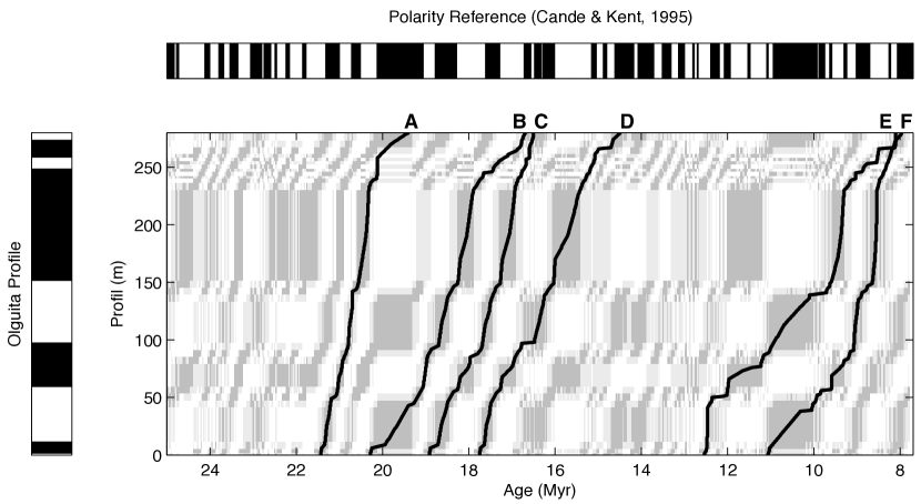
Figure 60: CRP between the polarity data of the Olguita profile and the reference data according to [203]. The used neighbourhood criterion is FAN with 30% RR (grey RP) and 40% RR (bright grey RP). In the polarity data the white colour marks a polarity of the Earth’s magnetic field in the present, whereas the black colour marks a reversal. Six potential LOS are found (A–F, corresponding to the potential LOS given in Fig. 61) [54].

A CRP is computed from these two data series by using an embedding dimension $m=4$, a delay of $\tau=6$ and a neighbourhood criterion of FAN (30% recurrence rate). Varying degrees of continuous lines between 21 and 16 Myr BP and between 12 and 8 Myr BP occur in the CRP, which can be interpreted as the desired LOS (Fig. 60). We will analyse six of these possibilities for the LOS. The search for the potential LOS is conducted using the algorithm described in the Appendix B.1. Moreover, we can evaluate the quality of these potential LOS by introducing a quality factor that takes into consideration the amount of gaps $N_{\circ}$ and black dots $N_{\bullet}$ on this line

$$Q=\frac{N_{\bullet}}{N_{\bullet}+N_{\circ}}\ 100\%.$$ (124)

The larger $Q$ is, the better the LOS is; $Q=100$% stands for an absolute continuous line. Moreover, the obtained LOS can be interpreted as the sedimentation rate (Fig. 61). Abrupt changes in the sedimentation rate are not expected, thus, the potential LOS should not change abruptly. As a criterion we can use hence the averaged second derivative with respect to the time $\langle\partial_{t}^{2}\rangle$.

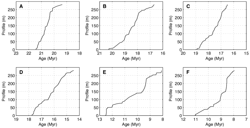
Figure 61: Potential LOS of the CRP presented in Fig. 60. They correspond to the potential sedimentation rates of the Olguita profile and mark sequences in the polarity reference, which match with the Olguita profile [54]. Due to this matching, the Olguita profile can be dated.

Table 5: Possible ages of the Olguita profile, which are based on the found potential LOS (Fig. 61) and characteristics of these potential LOS [54].

Plot	Age (Myr)	$N_{\bullet}$	$N_{\circ}$	$Q$ (%)	$\langle\partial_{t}^{2}\rangle$
A	19.4–21.4	345	23	93.8	5.5
B	16.7–20.3	407	43	90.4	12.5
C	16.5–18.9	351	15	95.9	5.0
D	14.4–17.8	392	16	96.1	20
E	8.1–12.6	482	16	96.8	23
F	7.9–11.1	399	13	96.8	18

The potential LOS differ slightly in the $Q$ factor, but strongly in the occurrence of abrupt changes in their slope (Fig. 61 and Tab. 5). The LOS in Fig. 61C has the smallest $\langle\partial_{t}^{2}\rangle$ and could be, therefore, a good LOS for the dating of the Olguita profile. Regarding this result, the Olguita profile would have an age between 16.5 and 18.9 Myr and an age-depth relation as it is represented by the LOS in Fig. 61C. Warkus’ investigation reveals the same result [202], although he also mentioned that the dating based on the polarity data is ambiguous. The alternative profile A has a similar good $Q$ value, but reveals an abrupt change in its slope around 20 Myr.

The stated results are only potential sequences and do not lay claim to absolute correctness. The example was presented just to illustrate the potentials of CRPs. In general, for such geological tasks as presented in the two previous applications, the distance matrix, Eq. (26), might be more appropriate.

4.5 Finding of nonlinear interrelations in palaeo-climate archives

Now we apply CRPs to geology and palaeo-climatology, where, as we have already seen, data are characterised by short length and non-stationarity. Such kind of data is rather typical in earth science, because of the unique character of, e. g., outcrops or drilling cores, which does not usually allow to repeat or refine a measurement.

A higher variability in rainfall and river discharge was discussed to be a reason for a sudden increase of the amount of landslides in NW Argentina 30,000 ¹⁴C years ago. A potential cause of the higher variability in rainfall is the El Niño/Southern Oscillation, represented by the Southern Oscillation Index (SOI). In order to support this hypothesis, annual layered lake sediments from the Santa Maria Basin (Province Salta, NW Argentina) with an age of 30,000 ¹⁴C years were compared with the El Niño dynamics from today. The colour variation of the lake sediments comes from reworked older sediments which are eroded and deposited only during extreme rainfall events, and, therefore, provides an archive of the precipitation variability [204, 205].

We compare the present-day SOI data with the palaeo-rainfall data in two steps. At first, the similarity between the SOI and modern rainfall is studied by using CRPs. Then, the similarity structure derived from the CRP of the SOI and the palaeo-rainfall is computed and compared with the similarity structure between the present-day data [7].

For the assessment of the modern El Niño/Southern Oscillation influence on local rainfall in NW Argentina, the monthly precipitation data from the station San Salvador de Jujuy (JUY) is used. The CRP analysis of JUY and SOI reveals clear positive values for the measures $RR^{c}_{\tau}$ and $L^{c}_{\tau}$ around a lag of zero and negative values after 8–12 months, which suggests a significant link between Jujuy rainfall and the El Niño/Southern Oscillation ( Fig. 62 A, C). The comparison between SOI and the 30,000 ¹⁴C year old precipitation data yields one maximum and two minimum values for $RR^{c}_{\tau}$ and $L^{c}_{\tau}$ for delays of about zero and ten months, similar to those found for JUY (Fig. 62B, D).

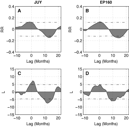
Figure 62: $RR^{c}_{\tau}$ and $L^{c}_{\tau}$ measures of the CRPs between SOI and precipitation in Jujuy (A, C) and palaeo-precipitation (B, D). Extreme values reveal high similarity between the dynamics of the rainfall and the ENSO [7].

The similarity between the time series of the modern rainfall data and the palaeo-precipitation record from the lake sediments suggests that an El Niño-like oscillation was active around 30,000 ¹⁴C years ago (roughly corresponding to 34,000 cal. years BP), which corresponds with the results of the investigation of Coccolithophores production [206]. In the semiarid basins of the NW Argentine Andes, the El Niño-like variation could have caused significant fluctuations in local rainfall around 30,000 ¹⁴C years ago similar to modern conditions, and, hence, could help to explain more frequent landsliding approximately 34,000 years ago in the semiarid basins of the Central Andes.

4.6 Automatised computation of $K_{2}$ applied to the stability of extra-solar planetary systems

The stability of extra-solar planetary systems is a central question of astrobiology. This kind of studies are important for future space missions dedicated to find habitable terrestrial planets in other stellar systems. The extra-solar planetary systems Gl 777 A, HD 72659, Gl 614, 47 Uma and HD 4208 are examined using extensive numerical experiments, concerning the question of whether they could host terrestrial-like planets in their habitable zones (HZ) [4].

Besides the study of the mean motion resonance between fictitious terrestrial planets and the existing gas giants in these five extra-solar systems, the stability of their orbits are investigated. A fine grid of initial conditions for a potential terrestrial planet within the HZ is chosen for each system, from which the stability of orbits is then assessed by direct integration over a time interval of one million years. For each of the five systems the two-dimensional grid of initial conditions contains 80 eccentricity points for the Jovian planet and up to 160 semimajor axis points for the fictitious planet. The equations of motion are integrated using a Lie-series integration method with an adaptive step size control.

The stability of orbits is examined by means of two different methods: $K_{2}$ estimated from RPs (Subsec. 3.6.1) and the maximum eccentricity achieved by the planet over the one million year integration. The eccentricity is an indication of the habitability of a terrestrial planet in the HZ; any value of $e>0.2$ produces a significant temperature difference on a planet’s surface between apoapse and periapse. Here we summarise the results obtained for the extra-solar planetary system Gl 777 A, which is a wide binary with a very large separation (3000 AU). Hence, there is no need to take the perturbations of the very far companion into account.

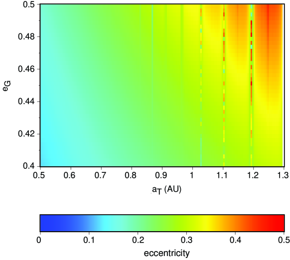
Figure 63: Initial condition diagram for fictitious planets in the system Gl 777 A: initial semimajor axes of the planet versus the eccentricity of the Jovian planet. The maximum eccentricity of an orbit during its dynamical evolution is colour-coded.

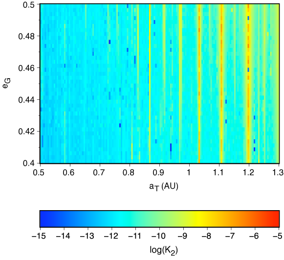
Figure 64: Initial condition diagram for fictitious planets in the system Gl 777 A: initial semimajor axes of the planet versus the eccentricity of the Jovian planet. The value of the $K_{2}$ of an orbit is colour-coded.

Considering the maximum eccentricity, high order resonance can be found (Fig. 63). Furthermore, unstable orbits due to high eccentricity and high semimajor axes values can be determined (red or yellow colours in Fig. 63). The latter feature is due to the larger perturbations near to the existing planet. The maximum eccentricity indicates the variable distance to the central star and consequently it is an indirect measure of the differential energy flux (insolation) on the planet. Therefore, it is possible to determine where the variation of this distance does not exceed 50%, corresponding to an eccentricity of $e=0.2$.

On the other hand, the correlation entropy $K_{2}$ is a more sensitive measure for the predictability of the orbit (Fig. 64). In particular, high order resonance is clearly indicated using this method, even in the case that the resonance is acting when the eccentricity of the planet is as low as $e=0.4$ (bottom of Fig. 64). $K_{2}$ was estimated using the automated algorithm described in the Appendix B.4.

Hence, we can conclude that both methods for the quantification of the stability of the orbits complement each other. From this analysis it can be inferred, that the planets in the system Gl 777 A will last long enough in the HZ to acquire the necessary conditions for life in the region with $a<1$ AU [4].

4.7 Synchronisation analysis of experimental data by means of RPs

As mentioned in Subsec. 3.8, many natural and laboratory systems are ill-phase defined or non-phase-coherent, i. e. they posses multiple time scales. In such cases, the RP based method for the synchronisation analysis is appropriate. To illustrate the application of this method to experimental data, we first show the results of the synchronisation analysis of two coupled electrochemical oscillators which exhibit non-phase coherent dynamics [151, 207, 208]. In this experiment the coupling strength between the electrochemical oscillators can be systematically varied. Hence, it is an active experiment.

Second, we apply the recurrence based synchronisation analysis to a passive experiment. We consider the synchronisation between the left and right fixational eye movements. The coupling strength between both eyes cannot be changed systematically, and hence, a hypothesis test has to be performed to get statistical significant results.

4.7.1 Synchronisation of electrochemical oscillators

We consider a laboratory experiment in which the synchronisation between electrochemical oscillators can be studied [209]. In this experiment, the electro-dissolution of iron in sulphuric acid cause non-phase coherent, chaotic current oscillations (Fig. 65). A standard three-compartment electrochemical cell consisting of two iron working electrodes, a Hg/Hg₂ SO₄/K₂SO₄ reference electrode, and a Pt mesh counter-electrode is used (the detailed experimental setup can be found in [210, 211]). The experiment is carried out in H₂SO₄. The applied potential of both electrodes is held at the same value using a potentiostat. Zero restiance ammeters are used to measure the currents of the electrodes. The coupling strength $\mu$ between the electrochemical oscillators can be varied by changing the connected resistors between the electrodes and the potentiostat [207]. We compute the two indices $CPR$ and $JPR$ for PS respectively GS for six different values of the coupling strength $\mu=\{0.0,0.2,0.4,0.6,0.8,1.0\}$.

Figure 65: Current of two non-phase-coherent electrochemical oscillators over time for coupling strength $\mu=0$ (solid: first, dashed: second electrode).

The transition to PS and GS is detected simultaneously at the coupling strength $\mu=0.6$ (Fig. 66A, B). This is in accordance with theoretical results, which confirm that the transition to PS and GS occurs almost simultaneously for non-phase coherent oscillators [150].

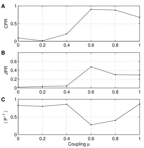
Figure 66: (A) $CPR$ index for PS, (B) $JPR$ index for GS and (C) $\langle P^{-1}\rangle$ index for GS (method of mutual false nearest neighbors) in dependence on the coupling strength $\mu$ of two non-phase-coherent electrochemical oscillators.

In contrast, the method of mutual false nearest neighbors (MFNN) [135, 153, 137] does not yield plausible results in this case. The index $\langle P^{-1}\rangle$ is the inverse of the mean value of the MFNN parameter. This index is zero for systems that are not in GS, and approximately one for systems in GS [135, 137, 153]. The index $\bar{P}^{-1}$ indicates GS for no coupling,$\mu=0$ (Fig. 66C), but for coupling strength $\mu=0.6$, where the other two indices $CPR$ and $JPR$ indicate synchronisation (Fig. 66A, B), $\langle P^{-1}\rangle$ does not. Hence, in the case of non-coherent oscillators the method of MFNN does not yield reliable results. (We used a total of 25,000 data points, $T_{r}=T_{d}=0.035~s$, i. e. a sampling rate of 2 kHz), $d_{r}=5$ and $d_{d}=12$. The measure $P(n,d_{r},d_{d})$ was computed at 10,000 different locations on the attractor and was used to evaluate the average values $\langle\bar{P}(d_{r},d_{d})\rangle$.)

4.7.2 Synchronisation analysis of cognitive data

Now we present the application of the RP based synchronisation analysis to a passive experiment, namely, the synchronisation between right and left eye movements during the fixation on one point. In this cognitive experiment, the coupling strength between both eyes cannot be varied systematically. Hence, a hypothesis test based on twin surrogates (Subsec. 3.10) is performed to get the statistical significance of the obtained results.

During fixation of a stationary target, our eyes perform small involuntary and allegedly erratic movements to counteract retinal adaptation. If these eye movements are experimentally suppressed, retinal adaptation to the constant input induces very rapid perceptual fading [212]. The fixational movements of the left and right eye are correlated very poorly at best [213]. Therefore, it is highly desirable to examine these processes from a perspective of PS.

The analysis of several trials and subjects has been presented in [214]; here we concentrate on the results for one subject and one trial. In each trial the subject fixates a small stimulus (black square on a white background, $3\times 3$ pixels on a computer display) with a spatial extent of $0.12^{\circ}$. Eye movements are achieved using an EyeLink-II system (SR Research, Osgoode, Ontario, Canada) with a sampling rate of 500 Hz and an instrumental spatial resolution less than $0.005^{\circ}$. The horizontal and vertical component of the eye movements are recorded (Fig. 67).

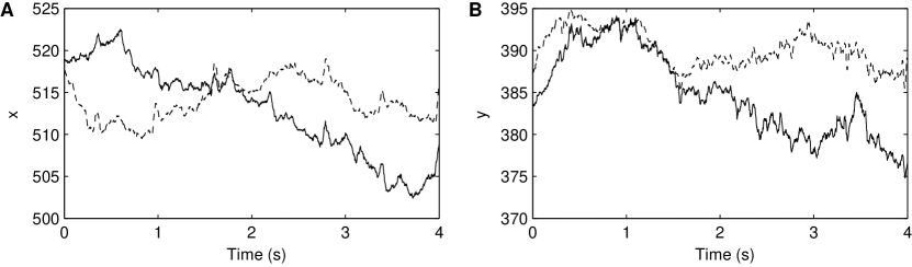
Figure 67: Simultaneous recording of left (solid) and right (dashed) fixational eye movements: (A) horizontal component (B) vertical component.

The data are first high-pass filtered applying a difference filter $\tilde{x}(t)=x(t)-x(t-\tau)$ with $\tau=40$ ms in order to eliminate the slow drift of the data. After this filtering, the trajectory is oscillating with maximum spectral power in the frequency range between 3 and 8 Hz (Fig. 68A, B). However, the trajectories of the eye movements are rather noisy and non-phase coherent. Therefore, it is cumbersome to estimate the phase of these data and, hence, the application of the recurrence based measure $CPR$ is appropriate.

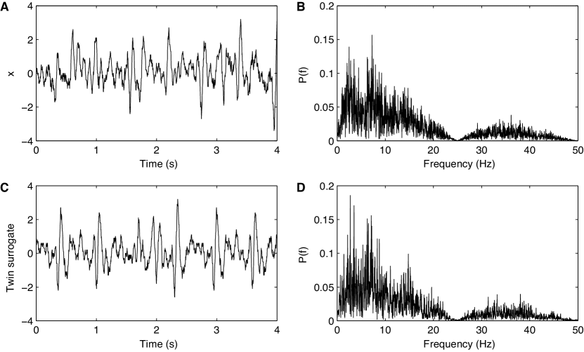
Figure 68: Filtered horizontal component of the left eye of one participant (A) and its corresponding periodogram (B). (C) Horizontal component of one surrogate of the left eye and (D) its corresponding periodogram.

For one trial of one participant, we obtain $CPR=0.911$. Even though this value is high (the maximal value that $CPR$ can take is 1), a hypothesis test should be performed in order to get statistically significant results. The hypothesis test is carried out by computing 200 twin surrogates of the left eye’s trajectory (cf. Subsec. 3.10). At a first glance, the characteristics of the original time series are well reproduced by the twin surrogate (Fig. 68C). The structure of the corresponding periodogram is also qualitatively reproduced (Fig. 68D). Note that the periodogram of the twin surrogate is not identical with the one of the original time series. This is because the twin surrogates correspond to another realisation of the same underlying process (respectively another trajectory starting at different initial conditions of the same underlying dynamical system) and the periodiograms of different realisation of a process differ slightly.

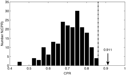
Figure 69: Histogram of the PS index $CPR$ of 200 twin surrogates (for one trial of one participant). The $CPR$ index for the original data (arrow) is significantly different from the one of the surrogates (dashed: 99% significance border of the rank order statistics).

Then, the synchronisation index $CPR$ between each twin surrogate of the left eye and the measured right eye’s trajectory is computed. The PS index of the original data is significantly different ($p<0.01$) from those of the surrogates (Fig. 69), which strongly indicates that the concept of PS can be successfully applied to study the interaction between the trajectories of the left and right eye during fixation. This result also suggests that the physiological mechanism in the brain that produces the fixational eye movements controls both eyes simultaneously, i. e. there might be only one centre in the brain that produces the fixational movements in both eyes or a close link between two centres. This finding of PS between left and right eyes is in good agreement with current knowledge of the physiology of the oculomotor circuitry.

Appendix A Mathematical models

Here we list the mathematical models used in the examples of this paper:

• Auto-regressive process first order

  $$x_{i}=a\,x_{i-1}+\xi_{i},$$ (125)

  where $\xi_{i}$ is white noise.

• 2D auto-regressive process second order

  $$x_{i,j}=\sum_{k,l=1}^{2}a_{k,l}\,x_{i-k,j-l}+\xi,$$ (126)

  where $\xi$ is white noise.

• The logistic map

  $$x_{i}=a\,x_{i-1}\left(1-x_{i-1}\right).$$ (127)

• The Bernoulli map

  $$x_{i}=2\,x_{i-1}\mod(1).$$ (128)

• The Rössler system [215]

  $$\dot{x} = -y-z,$$

  $$\dot{y} = x+a\,y,$$ (129)

  $$\dot{z} = b+z\,(x-c).$$

• The Lorenz system [78]

  $$\dot{x} = -\sigma(x-y),$$

  $$\dot{y} = -xz+rx-y,$$ (130)

  $$\dot{z} = xy-bz.$$

• Two Rössler systems mutually coupled by the first component

  $$\dot{x}_{1} = -(1+\nu)x_{2}-x_{3}+\mu(y_{1}-x_{1}),$$

  $$\dot{x}_{2} = (1+\nu)x_{1}+a\,x_{2},$$ (131)

  $$\dot{x}_{3} = b+x_{3}\,(x_{1}-c),$$

  $$\dot{y}_{1} = -(1-\nu)y_{2}-y_{3}+\mu(x_{1}-y_{1}),$$

  $$\dot{y}_{2} = (1-\nu)y_{1}+a\,y_{2},$$ (132)

  $$\dot{y}_{3} = b+y_{3}\,(y_{1}-c).$$

• Two Rössler systems mutually coupled by the second component

  $$\dot{x}_{1} = -(1+\nu)x_{2}-x_{3},$$

  $$\dot{x}_{2} = (1+\nu)x_{1}+a\,x_{2}+\mu(y_{2}-x_{2}),$$ (133)

  $$\dot{x}_{3} = b+x_{3}\,(x_{1}-c),$$

  $$\dot{y}_{1} = -(1-\nu)y_{2}-y_{3},$$

  $$\dot{y}_{2} = (1-\nu)y_{1}+a\,y_{2}+\mu(x_{2}-y_{2}),$$ (134)

  $$\dot{y}_{3} = b+y_{3}\,(y_{1}-c).$$

• The Lorenz system driven by a Rössler system

  $$\dot{x}_{1} = b+x_{1}(x_{2}-c),$$

  $$\dot{x}_{2} = -x_{1}-x_{3},$$ (135)

  $$\dot{x}_{3} = x_{2}+ax_{3},$$

  $$\dot{y}_{1} = -\sigma(y_{1}-y_{2}),$$

  $$\dot{y}_{2} = r\,u-y_{2}-u\,y_{3},$$ (136)

  $$\dot{y}_{3} = u\,y_{2}-b\,y_{3},$$

  where $u=x_{1}+x_{2}+x_{3}$.

Appendix B Algorithms

B.1 Algorithm to fit the LOS

The extraction of the LOS from the CRP in Subsecs. 3.3 and 4.4 was performed by using the following simple two-step algorithm. The set of indices of recurrence points $\mathbf{R}_{i_{\alpha},j_{\beta}}=1$ is denoted by $\{(i_{\alpha},j_{\beta})\}_{\alpha,\beta\in\mathds{N}}$. Those recurrence points $\mathbf{R}_{i_{\tilde{\alpha}},j_{\tilde{\beta}}}$ belonging to the LOS are denoted by $\{(i_{\tilde{\alpha}},j_{\tilde{\beta}})\}_{\tilde{\alpha},\tilde{\beta}\in\mathds{N}}$.

1. Find the recurrence point $(i_{1},j_{1})$ next to the axes origin. This is the first point of the LOS.

2. Find the next recurrence point at $(i_{\alpha},j_{\beta})$ after a previous determined LOS point $(i_{\tilde{\alpha}},j_{\tilde{\beta}})$ by looking for recurrence points in a squared window of size $w=2$, located at $(i_{\tilde{\alpha}},j_{\tilde{\beta}})$. If the edge of the window meets a recurrence point $(i_{\alpha},j_{\beta})$, we follow we step (3), else we iteratively increase the size of the window.

3. If there are subsequent recurrence points in $y$-direction ($x$-direction), the size $w$ of the window is iteratively increased in $y$-direction ($x$-direction) until a predefined size $(w+\Delta w)\times(w+\Delta w)$ ($\Delta w<dx,\Delta w<dy$) or until no new recurrence points are met. Using $\Delta w$ we compute the next LOS point $(i_{\tilde{\alpha}+1},j_{\tilde{\beta}+1})$ by determination of the centre of mass of the cluster of recurrence points with $i_{\tilde{\alpha}+1}=i_{\tilde{\alpha}}+(w+\Delta w)/2$ and $j_{\tilde{\beta}+1}=j_{\tilde{\beta}}+(w+\Delta w)/2$. This avoids that the algorithm places the LOS around widespread areas of recurrence points, but locates the LOS within these areas. This can be controlled by the two additional parameter $dx$ and $dy$. The next step is to set the LOS point $(i_{\tilde{\alpha}+1},j_{\tilde{\beta}+1})$ to the new starting point and to return to the step (2). These steps are repeated until the end of the RP is reached.

This algorithm is merely one of many possibilities. Its application should be carefully performed. The following criteria should be met in order to obtain a good LOS. The amount of targeted recurrence points by the LOS $N_{\bullet}$ should converge to the maximum and the amount of gaps in the LOS $N_{\circ}$ should converge to the minimum. An analysis with various estimated LOS confirms this requirement. The correlation between two LOS-synchronised data series arises with $N_{\bullet}$ and with $1/N_{\circ}$ (the correlation coefficient correlates best with the ratio $N_{\bullet}/N_{\circ}$).

This algorithm for the reconstruction of the LOS is implemented in the CRP toolbox for Matlab^® (provided by TOCSY: http://tocsy.agnld.uni-potsdam.de).

B.2 Algorithm for the reconstruction of a time series from its RP

The reconstruction algorithm (cf. Subsec. 3.9) consists of three main phases and a total of nine steps:

1. Determine the set difference $\mathcal{R}_{j}\setminus\mathcal{R}_{i}$

   1. If $n$ columns of the matrix $\mathbf{R}_{i,j}$ are identical, store their indices and remove $n-1$ of them, so that every column is unique.

   2. Determine for each recurrence point at $(i,j)$ the number of neighbours of $x_{j}$ which are not neighbours of $x_{i}$, i. e. the number of elements in the set difference $\mathcal{R}_{j}\setminus\mathcal{R}_{i}$. This number is denoted as $\mathbf{N}_{i,j}$ and can be calculated by $\sum_{k}(1-\mathbf{R}_{i,k})\,\mathbf{R}_{j,k}$.

   3. There exist exactly two points at $j_{1}$ and $j_{2}$, such that $\mathbf{N}_{i,j_{1/2}}=0\quad\forall i$. These two points correspond to the maximum and the minimum of the time series. Choose one of these two indices as starting point $k$ and assign the first element of the rank order series $r_{1}^{\text{ord}}=k$.

2. Iteration

   1. Look for the position of the minimum in the set $\{\mathbf{N}_{i,k}\}_{i}$.

      1. If the minimum is unique, i. e. there is one $j$ such that $\mathbf{N}_{j,k}<\mathbf{N}_{i,k}\quad\forall i\neq j$, the next point is then $k=j$.

      2. If the minimum is not unique, i. e. there is a set of $m$ indices $\{j_{1},\ldots,j_{m}\}$, so that $\mathbf{N}_{j_{1},k}=\ldots=\mathbf{N}_{j_{m},k}\leq\mathbf{N}_{i,k}\quad\forall i$, look for the position of the minimum in the set $\{\mathbf{N}_{k,j_{i}}\}_{i}$. This position will be the next point $k$.

   2. Add $k$ to the rank order series $r_{i}^{\text{ord}}$.

   3. Go to step (II4) until all indices are ranked.

3. Final Reconstruction

   1. Generate random numbers so that for each entry in the ordered series $r_{i}^{\text{ord}}$ is one random number, and rank order these numbers to the series $y_{i}$.

   2. Generate the time series $x_{i}$ by assigning $x_{r_{i}^{\text{ord}}}=y_{i}$.

   3. Reintroduce at the position of the “identical columns” obtained in step (I1) the values of the points at the corresponding indices which remained in the RP.

B.3 Twin Surrogates algorithm

A twin surrogate (cf. Subsec. 3.10) trajectory $\vec{x}^{s}_{i}$ of $\{\vec{x}_{i}\}_{i=1}^{N}$ is generated in the following way:

1. Identify all pairs of twins.

2. Choose an arbitrary starting point, e. g. $\vec{x}^{s}_{1}=\vec{x}_{j}$. Set index $i=2$.

3. 1. If $\vec{x}_{j}$ has no twin, the next point of the surrogate trajectory is $\vec{x}^{s}_{i}=\vec{x}_{j+1}$.

   2. If $\vec{x}_{j}$ has a twin at $\vec{x}_{k}$, either proceed with $\vec{x}^{s}_{i}=\vec{x}_{j+1}$ or $\vec{x}^{s}_{i}=\vec{x}_{k+1}$ with equal probability (if triplets occur proceed analogously).

4. Increase $i=i+1$ and go back to step (3) until the surrogate time series has the same length as the original one.

B.4 Automatisation of the $K_{2}$ estimation by RPs

For many applications, e. g., if spatio-temporal data has to be analysed, it is desirable to automate the algorithm to estimate $K_{2}$ based on RPs (Subsec. 3.6.1). Such an automated algorithm is also more objective, as otherwise the choice of the proper scaling regions of $p_{c}(\varepsilon,l)$ (Eq. 72) depends to some extent on the choice of the data analyst.

For the practical application, at first, the cumulative distribution of diagonals $p_{c}(\varepsilon,l)$ (the probability to find a diagonal of at least length $l$ in the RP) has to be calculated for different thresholds $\varepsilon$. The question arises, which values of $\varepsilon$ should be considered. As each system has its proper amplitude, which may differ from one system to another one, the choice will be different for each case and it is subjected to some arbitrariness. To overcome this problem, the value of the recurrence rate $RR$, Eq. (41), should be fixed, because it is normalised, and then calculate the corresponding $\varepsilon$ (cf. Subsec. 3.2.2). Using this choice of $\varepsilon$, the arbitrariness of choosing appropriate values for $\varepsilon$ is avoided and the same procedure of the estimation of $p_{c}(\varepsilon,l)$ can be applied for all systems.

The next step is crucial for the automatisation: the scaling region of $\ln p_{c}(RR,l)$ vs. $l$ and the plateau in $K_{2}(RR)$ vs. $RR$ must be estimated automatically. In both cases it is possible to apply a cluster dissection algorithm [216], which divides the set of points into distinct clusters. In each cluster a linear regression is performed. The algorithm minimises the sum of all square residuals in order to determine the scaling region and the plateau. To find both regions automatically, the following settings have been found to be appropriate [4]:

• Only diagonal lines up to a fixed length $l_{\max}$ are considered. Longer lines are excluded because of finite size effects. Reasonable values of $l_{\max}$ are at about 10% of the length of the time series.

• Only values of $p_{c}(RR,l)$ with $N^{2}p_{c}(RR,l)>500$ are regarded to obtain a reliable statistic.

• About 100 different values for $\varepsilon$ might be considered, corresponding to 100 equally spaced recurrence rates $RR$ between 1% and 99%, to have a good defined plateau in $K_{2}(RR)$ vs. $RR$.

• Furthermore, the number of clusters have to be specified when applying the cluster dissection algorithm: for the detection of the scaling region in $\ln p_{c}(RR,l)$ vs. $l$, two different clusters seem to be a rather good choice. Then, the slope of the largest cluster should be used. For the detection of the plateau in $K_{2}(RR)$ vs. $RR$, three clusters should be chosen and the value of the cluster with the minimum absolute slope is then used.

The most relevant references for this report are marked with ▲.

References

- [1] H. Poincaré. Sur la probleme des trois corps et les équations de la dynamique. Acta Mathematica, 13:1–271, 1890. ▲.
- [2] J.-P. Eckmann, S. O. Kamphorst, and D. Ruelle. Recurrence Plots of Dynamical Systems. Europhysics Letters, 5:973–977, 1987. ▲.
- [3] J. Kurths, U. Schwarz, C. P. Sonett, and U. Parlitz. Testing nonlinearity in radiocarbon data. Nonlinear Processes in Geophysics, 1(1):72–75, 1994.
- [4] N. Asghari, C. Broeg, L. Carone, R. Casas-Miranda, J. C. Castro Palacio, I. Csillik, R. Dvorak, F. Freistetter, G. Hadjivantsides, H. Hussmann, A. Khramova, M. Khristoforova, I. Khromova, I. Kitiashivilli, S. Kozlowski, T. Laakso, T. Laczkowski, D. Lytvinenko, O. Miloni, R. Morishima, A. Moro-Martin, V. Paksyutov, A. Pal, V. Patidar, B. Pecnik, O. Peles, J. Pyo, T. Quinn, A. Rodriguez, C. Romano, E. Saikia, J. Stadel, M. Thiel, N. Todorovic, D. Veras, E. Vieira Neto, J. Vilagi, W. von Bloh, R. Zechner, and E. Zhuchkova. Stability of terrestrial planets in the habitable zone of gl 777 a, hd 72659, gl 614, 47 uma and hd 4208. Astronomy & Astrophysics, 426:353–365, 2004.
- [5] N. V. Zolotova and D. I. Ponyavin. Phase asynchrony of the north-south sunspot activity. Astronomy & Astrophysics, 449(1):L1–L4, 2006.
- [6] N. Marwan, M. Thiel, and N. R. Nowaczyk. Cross Recurrence Plot Based Synchronization of Time Series. Nonlinear Processes in Geophysics, 9(3/4):325–331, 2002.
- [7] N. Marwan, M. H. Trauth, M. Vuille, and J. Kurths. Comparing modern and Pleistocene ENSO-like influences in NW Argentina using nonlinear time series analysis methods. Climate Dynamics, 21(3–4):317–326, 2003.
- [8] T. K. March, S. C. Chapman, and R. O. Dendy. Recurrence plot statistics and the effect of embedding. Physica D, 200(1–2):171–184, 2005.
- [9] A. S. Elwakil and A. M. Soliman. Mathematical Models of the Twin-T, Wien-bridge and Family of Minimum Component Electronic Chaos Generators with Demonstrative Recurrence Plots. Chaos, Solitons & Fractals, 10(8):1399–1411, 1999.
- [10] J. M. Nichols, S. T. Trickey, and M. Seaver. Damage detection using multivariate recurrence quantification analysis. Mechanical Systems and Signal Processing, 20(2):421–437, 2006.
- [11] A. Giuliani and C. Manetti. Hidden pecularities in the potential energy time series of a tripeptide highlighted by a recurrence plot analysis: A molecular dynamics simulation,. Physical Review E, 53(6):6336–6340, 1996.
- [12] C. Manetti, A. Giuliani, M.-A. Ceruso, C. L. Webber Jr., and J. P. Zbilut. Recurrence analysis of hydration effects on nonlinear protein dynamics: multiplicative scaling and additive processes. Physics Letters A, 281(5–6):317–323, 2001.
- [13] J. P. Zbilut, M. Koebbe, H. Loeb, and G. Mayer-Kress. Use of Recurrence Plots in the Analysis of Heart Beat Intervals. In Proceedings of the IEEE Conference on Computers in Cardiology, Chicago, 1990, pages 263–266. IEEE Computer Society Press, 1991.
- [14] N. Marwan, N. Wessel, U. Meyerfeldt, A. Schirdewan, and J. Kurths. Recurrence Plot Based Measures of Complexity and its Application to Heart Rate Variability Data. Physical Review E, 66(2):026702, 2002. ▲.
- [15] J. E. Naschitz, I. Rosner, M. Rozenbaum, M. Fields, H. Isseroff H., J. P. Babich, E. Zuckerman, N. Elias, D. Yeshurun, S. Naschitz, and E. Sabo. Patterns of cardiovascular reactivity in disease diagnosis. QJM: An International Journal of Medicine, 97(3):141–151, 2004.
- [16] N. Thomasson, T. J. Hoeppner, C. L. Webber Jr., and J. P. Zbilut. Recurrence quantification in epileptic EEGs. Physics Letters A, 279(1–2):94–101, 2001.
- [17] N. Marwan and A. Meinke. Extended recurrence plot analysis and its application to ERP data. International Journal of Bifurcation and Chaos “Cognition and Complex Brain Dynamics”, 14(2):761–771, February 2004.
- [18] R. Acharya U., O. Faustand N. Kannathal, T. L. Chua, and S. Laxminarayan. Non-linear analysis of EEG signals at various sleep stages. Computer Methods and Programs in Biomedicine, 80(1):37–45, 2005.
- [19] A. Katok and B. Hasselblatt. Introduction to the Modern Theory of Dynamical Systems. Cambridge University Press, Cambridge, 1995.
- [20] H. M. van den Dool. Searching for analogues, how long must we wait? Tellus A, 46(3):314–324, 1994.
- [21] V. Balakrishnan, G. Nicolis, and C. Nicolis. Recurrence Time Statistics in Chaotic Dynamics. Stochastics and Dynamics, 1(3):345–359, 2001.
- [22] W. Feller. Fluctuationtheory of recurrent events. Transactions of American Mathematical Society, 67:98–119, 1949.
- [23] D. R. Cox and H. D. Miller. The theory of Stochastic Processes. Chapman and Hall, London, New York, 1994.
- [24] B. Pitskel. Poisson limit law for markov chains. Ergodic Theory and Dynamical Systems, 11:501–513, 1991.
- [25] Y. G. Sinai. Some mathematical problems in the theory of quantum chaos. Physica A, 163(1):197–204, 1970.
- [26] M. Hirata. Poisson law for axiom a diffeomorphisms. Ergodic Theory and Dynamical Systems, 13(3):533–556, 1993.
- [27] P. Collet, A. Galves, and B. Schmitt. Unpredictability of the occurrence time of a long laminar period in a model of temporal intermittency. Annales de l’Institut Henri Poincarè, 57(3):319–331, 1992.
- [28] M. Hirata. Poisson lawfor the dynamical systems with the “self-mixing” conditions. In Dynamical Systems and Chaos, volume 1, pages 87–96. World Scientific Publishing, River Edge, NJ, 1995.
- [29] M. Hirata, B. Saussol, and S. Vaienti. Statistics of Return Times: A General Framework and New Applications. Communications in Mathematical Physics, 206(1):33–55, 1999.
- [30] V. Penné, B. Saussol, and S. Vaienti. Dimensions for recurrence times: topological and dynamical properties. Discrete and Continuous Dynamical Systems A, 4(4):783–798, 1999.
- [31] V. Afraimovich. Pesin’s dimension for Poincaré recurrences. Chaos, 7(1):12–20, 1997. ▲.
- [32] V. Afraimovich, J.-R. Chazottes, and B. Saussol. Local dimensions for Poincaré recurrences. Electronic Research Announcements of the American Mathematical Society, 6:64–74, 2000.
- [33] V. Afraimovich, J.-R. Chazottes, and B. Saussol. Pointwise dimensions for Poincaré recurrences associated with maps and special flows. Discrete and Continuous Dynamical Systems A, 9(2):263–280, 2003.
- [34] J. B. Gao. Recurrence Time Statistics for Chaotic Systems and Their Applications. Physical Review Letters, 83(16):3178–3181, 1999.
- [35] L. Barreira and B. Saussol. Hausdorff dimension of measures via poincaré recurrence. Communications in Mathematical Physics, 219(2):443–463, 2001.
- [36] N. Hadyn, J. Luevano, G. Mantica, and S. Vaienti. Multifractal Properties of Return Time Statistics. Physical Review Letters, 88(22):224502, 2002.
- [37] B. Saussol and J. Wu. Recurrence spectrum in smooth dynamical systems. Nonlinearity, 16(6):1991–2001, 2003.
- [38] B. Saussol, S. Troubetzkoy, and S. Vaienti. Recurrence, Dimensions, and Lyapunov Exponents. Journal of Statistical Physics, 106(3–4):623–634, 2002.
- [39] B. Saussol, S. Troubetzkoy, and S. Vaienti. Recurrence and Lyapunov Exponents for diffeomorphisms. Moscow Mathematical Journal, 3(1):189–203, 2003.
- [40] L.-S. Young. Recurrence times and rates of mixing. Israel Journal of Mathematics, 110:153–188, 1999.
- [41] V. Balakrishnan, G. Nicolis, and C. Nicolis. Recurrence time statistics in deterministic and stochastic dynamical systems in continuous time: A comparison. Physical Review E, 61(3):2490–2499, 2000.
- [42] R. Gilmore and M. Lefranc. The Topology of Chaos: Alice in Stretch and Squeezeland. Wiley, New York, 2002.
- [43] N. H. Packard, J. P. Crutchfield, J. D. Farmer, and R. S. Shaw. Geometry from a Time Series. Physical Review Letters, 45(9):712–716, 1980.
- [44] F. Takens. Detecting Strange Attractors in Turbulence. In D. Rand and L.-S. Young, editors, Dynamical Systems and Turbulence, volume 898 of Lecture Notes in Mathematics, pages 366–381. Springer, Berlin, 1981.
- [45] T.Sauer, J. A. Yorke, and M. Casdagli. Embedology. Journal of Statistical Physics, 65(3–4):579–616, 1991.
- [46] H. Kantz and T. Schreiber. Nonlinear Time Series Analysis. University Press, Cambridge, 1997. ▲.
- [47] L. Cao. Practical method for determining the minimum embedding dimension of a scalar time series. Physica D, 110(1–2):43–50, 1997.
- [48] G. M. Mindlin and R. Gilmore. Topological analysis and synthesis of chaotic time series. Physica D, 58(1–4):229–242, 1992.
- [49] M. Koebbe and G. Mayer-Kress. Use of Recurrence Plots in the Analysis of Time-Series Data. In M. Casdagli and S. Eubank, editors, Proceedings of SFI Studies in the Science of Complexity, volume XXI, pages 361–378, Redwood City, 1992. Addison-Wesley.
- [50] J. P. Zbilut and C. L. Webber Jr. Embeddings and delays as derived from quantification of recurrence plots. Physics Letters A, 171(3–4):199–203, 1992. ▲.
- [51] J. P. Zbilut, J.-M. Zaldívar-Comenges, and F. Strozzi. Recurrence quantification based Liapunov exponents for monitoring divergence in experimental data. Physics Letters A, 297(3–4):173–181, 2002.
- [52] M. Thiel, M. C. Romano, J. Kurths, R. Meucci, E. Allaria, and F. T. Arecchi. Influence of observational noise on the recurrence quantification analysis. Physica D, 171(3):138–152, 2002.
- [53] L. Matassini, H. Kantz, J. Hołyst, and R. Hegger. Optimizing of recurrence plots for noise reduction. Physical Review E, 65(2):021102, 2002.
- [54] N. Marwan. Encounters With Neighbours – Current Developments Of Concepts Based On Recurrence Plots And Their Applications. PhD thesis, University of Potsdam, 2003.
- [55] N. Marwan and J. Kurths. Line structures in recurrence plots. Physics Letters A, 336(4–5):349–357, 2005. ▲.
- [56] N. Marwan and J. Kurths. Cross recurrence plots and their applications. In C. V. Benton, editor, Mathematical Physics Research at the Cutting Edge, pages 101–139. Nova Science Publishers, Hauppauge, 2004.
- [57] P. Grassberger and I. Procaccia. Measuring the strangeness of strange attractors. Physica D, 9(1–2):189–208, 1983. ▲.
- [58] J. Theiler. Spurious dimension from correlation algorithms applied to limited time-series data. Physical Review A, 34(3):2427–2432, 1986.
- [59] J. Kurths and H. Herzel. An attractor in a solar time series. Physica D, 25:165–172, 1987.
- [60] J. Gao and Z. Zheng. Direct dynamical test for deterministic chaos and optimal embedding of a chaotic time series. Physical Review E, 49:3807–3814, 1994.
- [61] A. Facchini, H. Kantz, and E. Tiezzi. Recurrence plot analysis of nonstationary data: The understanding of curved patterns. Physical Review E, 72:021915, 2005.
- [62] M. Thiel, M. C. Romano, and J. Kurths. Spurious Structures in Recurrence Plots Induced by Embedding. Nonlinear Dynamics, 44(1–4):299–305, 2006.
- [63] C. L. Webber Jr. Recurrence Quantification Analysis, 2003.
- [64] J. S. Iwanski and E. Bradley. Recurrence plots of experimental data: To embed or not to embed? Chaos, 8(4):861–871, 1998.
- [65] J.-P. Eckmann, S. Oliffson Kamphorst, D. Ruelle, and S. Ciliberto. Liapunov exponents from time series. Physical Review A, 34(6):4971–4979, 1986.
- [66] J. M. Choi, B. H. Bae, and S. Y. Kim. Divergence in perpendicular recurrence plot; quantification of dynamical divergence from short chaotic time series. Physics Letters A, 263(4–6):299–306, 1999.
- [67] S. Horai and T. Yamada K. Aihara. Determinism Analysis with Iso-Directional Recurrence Plots. IEEE Transactions - Institute of Electrical Engineers of Japan C, 122(1):141–147, 2002.
- [68] F. M. Atay and Y. Altıntaş. Recovering smooth dynamics from time series with the aid of recurrence plots. Physical Review E, 59(6):6593–6598, 1999.
- [69] D. P. Lathrop and E. J. Kostelich. Characterization of an experimental strange attractor by periodic orbits. Physical Review A, 40(7):4028–4031, 1989.
- [70] N. B. Tufillaro, H. G. Solari, and R. Gilmore. Relative rotation rates: Fingerprints for strange attractors. Physical Review A, 41(10):5717–5720, 1990.
- [71] R. Manuca and R. Savit. Stationarity and nonstationarity in time series analysis. Physica D, 99(2–3):134–161, 1996.
- [72] M. C. Casdagli. Recurrence plots revisited. Physica D, 108(1–2):12–44, 1997.
- [73] H. Kantz. Quantifying the closeness of fractal measures. Physical Review E, 49(6):5091–5097, 1994.
- [74] A. Groth. Visualization and detection of coupling in time series by order recurrence plots. Preprint series of the DFG priority program 1114 “Mathematical methods for time series analysis and digital image processing”, 67, December 2004.
- [75] A. Groth. Analyse der Wiederkehr in dynamischen Systemen auf einer Ordinalskala. PhD thesis, University of Greifswald, 2006.
- [76] R. Balasubramaniam, M. A. Riley, and M. T. Turvey. Specificity of postural sway to the demands of a precision task. Gait & Posture, 11(1):12–24, 2000.
- [77] Q. Huang and G. A. Sobolev. Precursory seismicity changes associated with the Nemuro Peninsula earthquake, January 28, 2000. Journal of Asian Earth Sciences, 21(2):135–146, 2002.
- [78] E. N. Lorenz. Deterministic Nonperiodic Flow. Journal of the Atmospheric Sciences, 20:120–141, 1963.
- [79] M. Kac. On the notion of recurrence in discrete stochastic processes. Bulletin of the American Mathematical Society, 53:1002–1010, 1947. ▲.
- [80] A. Provenzale, L. A. Smith, R. Vio, and G. Murante. Distinguishing between low-dimensional dynamics and randomness in measured time series. Physica D, 58(1–4):31–49, 1992.
- [81] M. B. Kennel. Statistical test for dynamical nonstationarity in observed time-series data. Physical Review E, 56(1):316–321, 1997.
- [82] C. Rieke, K. Sternickel, R. G. Andrzejak, C. E. Elger, P. David, and K. Lehnertz. Measuring Nonstationarity by Analyzing the Loss of Recurrence in Dynamical Systems. Physical Review Letters, 88:244102, 2002. ▲.
- [83] L. Rabiner and B.-H. Juang. Fundamentals of Speech Recognition. Prentice Hall, PTR, 1993.
- [84] H. Sakoe and S. Chiba. Dynamic programming algorithm optimization for spoken word recognition. IEEE Trans. Acoustics, Speech and Signal Proc., 26:43–49, 1978.
- [85] J. B. Kruskal. An overview of sequence comparison. In D. Sankoff and J. B. Kruskal, editors, Time Warps, String Edits, and Macromolecules: The Theory and Practice of Sequence Comparison, pages 1–44. Addison-Wesley, Reading, Mass., 1983.
- [86] J. V. Maizel and R. P. Lenk. Enhanced Graphic Matrix Analysis of Nucleic Acid and Protein Sequences. Proceedings of the National Academy of Sciences, 78(12):7665–7669, 1981.
- [87] M. Vihinen. An algorithm for simultaneous comparison of several sequences. Computer applications in the biosciences: CABIOS, 4(1):89–92, 1988.
- [88] M. Bernstein, J. D. Bolter, M. Joyce, and E. Mylonas. Architectures for volatile hypertext. In Proceedings of the third annual ACM conference on Hypertext, San Antonio, USA, pages 243–260, 1991.
- [89] R. Cutler and L. Davis. Robust Periodic Motion and Motion Symmetry Detection. In Proceedings of the Conference on Computer Vision and Pattern Recognition, South Carolina, USA, volume 2, page 2615, 2000.
- [90] M. A. Casey and W. Westner. Separation of mixed audio sources by independent subspace analysis. In Proceedings of the International Computer Music Conference (ICMC), Berlin, Germany, 2000.
- [91] J. Foote and M. Cooper. Visualizing Musical Structure and Rhythm via Self-Similarity. In Proceedings of the International Conference on Computer Music, Habana, Cuba, 2001.
- [92] H. S. Chan and K. A. Dill. Intrachain loops in polymers: Effects of excluded volume. Journal of Chemical Physics, 90(1):492–509, 1989.
- [93] E. Domany. Protein folding in contact map space. Physica A, 288(1–4):1–9, 2000.
- [94] L. Holm and C. Sander. Protein Structure Comparison by Alignment of Distance Matrices. Journal of Molecular Biology, 233(1):123–138, 1993.
- [95] J. P. Zbilut, A. Giuliani, and C. L. Webber Jr. Detecting deterministic signals in exceptionally noisy environments using cross-recurrence quantification. Physics Letters A, 246(1–2):122–128, 1998.
- [96] N. Marwan and J. Kurths. Nonlinear analysis of bivariate data with cross recurrence plots. Physics Letters A, 302(5–6):299–307, 2002. ▲.
- [97] A. Groth. Visualization of coupling in time series by order recurrence plots. Physical Review E, 72(4):046220, 2005.
- [98] N. Marwan. Untersuchung der Klimavariabilität in NW Argentinien mit Hilfe der quantitativen Analyse von Recurrence Plots. Master’s thesis, Dresden University of Technology, Dresden University of Technology, October 1999.
- [99] G. Rosenblum, A. S. Pikovsky, and J. Kurths. From Phase to Lag Synchronization in Coupled Chaotic Oscillators. Physical Review Letters, 78(22):4193–4196, 1997.
- [100] O. V. Sosnovtseva, A. G. Balanov, T. E. Vadivasova, V. V. Astakhov, and E. Mosekilde. Loss of lag synchronization in coupld chaotic systems. Physical Review E, 60(6), 1999.
- [101] C. L. Webber Jr. and J. P. Zbilut. Dynamical assessment of physiological systems and states using recurrence plot strategies. Journal of Applied Physiology, 76(2):965–973, 1994. ▲.
- [102] L. L. Trulla, A. Giuliani, J. P. Zbilut, and C. L. Webber Jr. Recurrence quantification analysis of the logistic equation with transients. Physics Letters A, 223(4):255–260, 1996.
- [103] R. Quian Quiroga, T. Kreuz, and P. Grassberger. Event synchronization: A simple and fast method to measure synchronicity and time delay patterns. Physical Review E, 66(4):041904, 2002.
- [104] R. Gilmore. Topological analysis of chaotic dynamical systems. Review of Modern Physics, 70(4):1455–1529, 1998.
- [105] J. H. Argyris, G. Faust, and M. Haase. An Exploration of Chaos. North Holland, Amsterdam, 1994.
- [106] P. Collet and J.-P. Eckmann. Iterated maps on the interval as dynamical systems. Birkhäuser, Basel Boston Stuttgart, 1980.
- [107] E. M. Oblow. Supertracks, supertrack functions and chaos in the quadratic map. Physics Letters A, 128(8):406, 1988.
- [108] P. Saparin, A. Witt, J. Kurths, and V. Anishchenko. The Renormalized Entropy–an Appropriate Complexity Measure? Chaos, Solitons & Fractals, 4(10):1907–1916, 1994.
- [109] R. Wackerbauer, A. Witt, H. Atmanspacher, J. Kurths, and H. Scheingraber. A Comparative Classification of Complexity Measures. Chaos, Solitons & Fractals, 4(4):133–173, 1994.
- [110] P. Grassberger and I. Procaccia. Estimation of the Kolmogorov entropy from a chaotic signal. Physical Review A, 9(1–2):2591–2593, 1983.
- [111] P. Grassberger. Generalized Dimensions of Strange Attractors. Physics Letters A, 97(6):227–230, 1983.
- [112] K. Pawelzik and H. G. Schuster. Generalized dimensions and entropies from a measured time series. Physical Review A, 35(1):481–484, 1987.
- [113] D. Prichard and J. Theiler. Generalised redundancies for time series analysis. Physica D, 84(3–4):476–493, 1995. ▲.
- [114] P. Faure and H. Korn. A new method to estimate the Kolmogorov entropy from recurrence plots: its application to neuronal signals. Physica D, 122(1–4):265–279, 1998. ▲.
- [115] M. Thiel, M. C. Romano, and J. Kurths. Analytical Description of Recurrence Plots of white noise and chaotic processes. Izvestija vyssich ucebnych zavedenij/ Prikladnaja nelinejnaja dinamika – Applied Nonlinear Dynamics, 11(3):20–30, 2003.
- [116] M. Thiel, M. C. Romano, P. L. Read, and J. Kurths. Estimation of dynamical invariants without embedding by recurrence plots. Chaos, 14(2):234–243, 2004. ▲.
- [117] D. Ruelle. An inequality for the entropy of differentiable maps. Bol. Soc. Bras. Mat., 9:83, 1978.
- [118] C. Beck and F. Schlögl. Thermodynamics of Chaotic Systems: An Introduction. Cambridge Nonlinear Science Series 4. Cambridge University Press, 2001.
- [119] A. Rényi. Probability theory. North-Holland, 1970.
- [120] P. Grassberger and I. Procaccia. Characterization of strange attractors. Physical Review Letters, 50(5):346–349, 1983.
- [121] K. T. Alligood, T. D. Sauer, and J. A. Yorke. Chaos, an introduction to dynamical systems. Springer, 1996.
- [122] V. S. Anishchenko, T. E. Vadivasova, J. Kurths, G. A. Okrokvertskhov, and G. I. Strelkova. Autocorrelation function and spectral linewidth of spiral chaos in a physical experiment. Physical Review E, 69:036215, 2004.
- [123] C. Raab and J. Kurths. Estimations of large-scale dimensions densities. Physical Review E, 64(1):0162161, 2001.
- [124] U. Hübner, C.-O. Weiss, N. Abraham, and D. Tang. Lorenz-like chaos in nh3-fir lasers (data set a). In Time Series Prediction: Forecasting the Future and Understanding the Past, pages 73–104. Addison-Wesley, Reading, MA, 1993.
- [125] M. Ding, C. Grebogi, E. Ott, and T. Sauer amd J. A. Yorke. Plateau onset for correlation dimension: When does it occur? Physics Review Letters, 70:3872–3875, 1993.
- [126] R. Pastor-Satorras and R. H. Riedi. Numerical estimates of the generalized dimensions of the Hénon attractor for negative q. Journal of Physics A: Mathematical and General, 29(15):L391–L398, 1996.
- [127] W. Liebert and H. G. Schuster. Proper choice of the time delay for the analysis of chaotic time series. Physics Letters A, 142(2–3):107–111, 1989.
- [128] D. B. Vasconcelos, S. R. Lopes, R. L. Viana, and J. Kurths. Spatial recurrence plots. Physical Review E, 73:056207, 2006.
- [129] N. Marwan, J. Kurths, and P. Saparin. Generalised Recurrence Plot Analysis for Spatial Data. Physics Letters A, in press.
- [130] H. Fujisaka and T. Yamada. Stability theory of synchronized motion in coupled-oscillator systems. Progress of Theoretical Physics, 69(1):32, 1983.
- [131] V. S. Afraimovich, N. N. Verichev, and M. I. Rabinovich. Stochastic synchronization of oscillation in dissipative systems. Izvestiya Vysshikh Uchebnykh Zavedenii Radiofizika, 29(9):1050–1060, 1986.
- [132] L. M. Pecora and T. L. Carroll. Synchronization in chaotic systems. Physical Review Letters, 64(8):821–824, 1990.
- [133] A. S. Pikovsky, M. G. Rosenblum, and J. Kurths. Synchronization: a universal concept in nonlinear sciences. Cambridge Nonlinear Science Series 12. Cambridge University Press, 2001.
- [134] S. Boccaletti, J. Kurths, G. Osipov, D. L. Valladares, and C. S. Zhou. The synchronization of chaotic systems. Physics Reports, 366(1-2):1–101, 2002.
- [135] N. F. Rulkov, M. M. Sushchik, L. S. Tsimring, and H. D. I. Abarbanel. Generalized synchronization of chaos in directionally coupled chaotic systems. Physical Review E, 51(2):98–994, 1995.
- [136] L. Kocarev, U. Parlitz, and T. Stojanovski. Generalized Synchronization of Chaotic Signals. In Proceedings of the International Symposium on Nonlinear Theory and Its Applications (NOLTA’95),, pages 953–956, 1995.
- [137] S. Boccaletti, D. L. Valladares, J. Kurths, D. Maza, and H. Mancini. Synchronization of chaotic structurally nonequivalent systems. Physical Review E, 61(4):3712–3715, 2000.
- [138] A. Kittel, A. Parisi, and K. Pyragas. Generalized synchronization of chaos in electronic circuit experiments. Physica D, 112(3–4):459–471, 1998.
- [139] G. D. van Wiggeren and R. Roy. Communication with Chaotic Lasers. Science, 279(5354):1198–1200, 1998.
- [140] L. Kocarev, K. S. Halle, K. Eckert, L. O. Chua, and U. Parlitz. Experimental demonstration of secure communications via chaotic synchronization. International Journal of Bifurcation and Chaos, 2(3):709–713, 1992.
- [141] C. M. Ticos, E. Rosa Jr., W. B. Pardo, J. A. Walkenstein, and M. Monti. Experimental Real-Time Phase Synchronization of a Paced Chaotic Plasma Discharge. Physical Review Letters, 85(14):2929–2932, 2000.
- [142] E. Allaria, F. T. Arecchi, A. Di Garbo, and R. Meucci. Synchronization of Homoclinic Chaos. Physical Review Letters, 86(5):791–794, 2001.
- [143] I. Z. Kiss and J. L. Hudson. Phase synchronization and suppression of chaos through intermittency in forcing of an electrochemical oscillator. Physical Review E, 64(4):046215, 2001.
- [144] C. Schaefer, M. G. Rosenblum, J. Kurths, and H. H. Abel. Heartbeat synchronized with ventilation. Nature, 392:239–240, 1998.
- [145] B. Blasius, A. Huppert, and L. Stone. Complex dynamics and phase synchronization in spatially extended ecological systems. Nature, 399:354–359, 1999.
- [146] P. Tass, M. G. Rosenblum, J. Weule, J. Kurths, A. Pikovsky, J. Volkmann, A. Schnitzler, and H.-J. Freund. Detection of phase locking from noisy data: Application to magnetoencephalography. Physical Review Letters, 81(15):3291–3294, 1998.
- [147] M. C. Romano, M. Thiel, J. Kurths, and W. von Bloh. Multivariate Recurrence Plots. Physics Letters A, 330(3–4):214–223, 2004. ▲.
- [148] M. G. Rosenblum, A. S. Pikovsky, and J. Kurths. Phase Synchronization of Chaotic Oscillators. Physical Review Letters, 76:1804, 1996.
- [149] M. G. Rosenblum, A. S. Pikovsky, J. Kurths, G. V. Osipov, I. Z. Kiss, and J. L. Hudson. Locking-Based Frequency Measurement and Synchronization of Chaotic Oscillators with Complex Dynamics. Physical Review Letters, 89(26):264102, 2002.
- [150] G. V. Osipov, B. Hu, C. Zhou, M. V. Ivanchenko, and J. Kurths. Three Types of Transitions to Phase Synchronization in Coupled Chaotic Oscillators. Physical Review Letters, 91(2):024101, 2003.
- [151] M. C. Romano, M. Thiel, J. Kurths, I. Z. Kiss, and J. Hudson. Detection of synchronization for non-phase-coherent and non-stationary data. Europhysics Letters, 71(3):466–472, 2005. ▲.
- [152] L. Kocarev and U. Parlitz. Generalized Synchronization, Predictability, and Equivalence of Unidirectionally Coupled Dynamical Systems. Physical Review Letters, 76(11):1816–1819, 1996.
- [153] J. Arnhold, P. Grassberger, K. Lehnertz, and C. E. Elger. A robust method for detecting interdependences: application to intracranially recorded EEG. Physica D, 134(4):419–430, 1999.
- [154] P. So, E. Barreto, K. Josic, E. Sander, and S. J. Schiff. Limits to the experimental detection of nonlinear synchrony. Physical Review E, 65(4):046225, 2002.
- [155] D. He, Z. Zheng, and L. Stone. Detecting generalized synchrony: An improved approach. Physical Review E, 67(2):026223, 2003.
- [156] H. D. I. Abarbanel, N. F. Rulkov, and M. M. Sushchik. Generalized synchronization of chaos: The auxiliary system approach. Physical Review E, 53(5):4528–4535, 1996.
- [157] T. Schreiber. Measuring Information Transfer. Physical Review Letters, 85(2):461–464, July 2000.
- [158] U. Parlitz and A. Hornstein. Detecting generalized synchronization from time series. In Fifth EUROMECH Nonlinear Dynamics Conference ENOC-2005, August 7-12, 2005, Eindhoven (Netherlands), pages 1174–1181, 2005.
- [159] S. Boccaletti and D. L. Valladares. Characterization of intermittent lag synchronization. Physical Review E, 62(5):7497–7500, 2000.
- [160] G. McGuire, N. B. Azar, and M. Shelhamer. Recurrence matrices and the preservation of dynamical properties. Physics Letters A, 237(1–2):43–47, 1997.
- [161] M. Thiel, M. C. Romano, and J. Kurths. How much information is contained in a recurrence plot? Physics Letters A, 330(5):343–349, 2004. ▲.
- [162] P. van Leeuwen, D. Geue, S. Lange, D. Cysarz, H. Bettermann, and D. H. W. Grönemeyer. Is there evidence of fetal-maternal heart rate synchronization? BMC Physiology, 3:2, 2003.
- [163] M. Thiel, M. C. Romano, J. Kurths, M. Rolfs, and R. Kliegl. Twin Surrogates to Test for Complex Synchronization. Physical Review Letters, subm.
- [164] E. Rodriguez, N. George, J.-P. Lachaux, J. Martinerie, B. Renault, and F. J. Varela. Perception’s shadow: long-distance synchronization of human brain activity. Nature, 397(6718):430–433, 1999.
- [165] Y. Kuramoto. Chemical oscillations, waves and turbulence. Springer-Verlag, New York, USA, 1984.
- [166] D. Auerbach, P. Cvitanovic, J.-P. Eckmann, G. Gunaratne, and I. Procaccia. Exploring chaotic motion through periodic orbits. Physical Review Letters, 58:2387, 1987.
- [167] E. Bradley and R. Mantilla. Recurrence plots and unstable periodic orbits. Chaos, 12(3):596–600, 2002.
- [168] P. So, T. Sauer, B. Gluckman, C. Grebogi, and S. Schiff. Extracting unstable periodic orbits from chaotic time series data. Physical Review E, 55:5398, 1997.
- [169] K. Urbanowicz and J. A. Hołyst. Noise-level estimation of time series using coarse-grained entropy. Physical Review E, 67:046218, 2003.
- [170] C. L. Webber Jr., M. A. Schmidt, and J. M. Walsh. Influence of isometric loading on biceps EMG dynamics as assessed by linear and nonlinear tools. Journal of Applied Physiology, 78(3):814–822, 1995.
- [171] M. Shelhamer. On the correlation dimension of optokinetic nystagmus eye movements: computational parameters, filtering, nonstationarity, and surrogate data. Biological Cybernetics, 76(4):237–250, 1997.
- [172] M. A. Riley, R. Balasubramaniam, and M. T. Turvey. Recurrence quantification analysis of postural fluctuations. Gait & Posture, 9(1):65–78, 1999.
- [173] A. Babloyantz. Evidence for slow brain waves: a dynamical approach. Electroencephalography and Clinical Neurophysiology, 78(5):402–405, 1991.
- [174] P. Faure and H. Korn. Is there chaos in the brain? I. Concepts of nonlinear dynamics and methods of investigation. Comptes Rendus de l’Academie des Sciences - Series III - Sciences de la Vie, 324(9):773–793, 2001.
- [175] C. Frontali and E. Pizzi. Similarity in oligonucleotide usage in introns and intergenic regions contributes to long-range correlation in the Caenorhabditis elegans genome. Gene, 232(1):87–95, 1999.
- [176] Z.-B. Wu. Recurrence plot analysis of DNA sequences. Physics Letters A, 332(3–4):250–255, 2004.
- [177] D. Vretenar, N. Paar, P. Ring, and G. A. Lalazissis. Nonlinear dynamics of giant resonances in atomic nuclei. Physical Review E, 60(1):308–319, 1999.
- [178] M. Rustici, C. Caravati, E. Petretto, M. Branca, and N. Marchettini. Transition Scenarios during the Evolution of the Belousov-Zhabotinsky Reaction in an Unstirred Batch Reactor. Journal of Physical Chemistry A, 103(33):6564–6570, 1999.
- [179] H. Castellini and L. Romanelli. Applications of recurrence quantified analysis to study the dynamics of chaotic chemical reaction. Physica A, 342(1–2):301–307, 2004.
- [180] A. Giuliani and M. Tomasi. Recurrence quantification analysis reveals interaction partners in paramyxoviridae envelope glycoproteins. Proteins: Structure, Function, and Genetics, 46(2):171–176, 2002.
- [181] W. von Bloh, M. C. Romano, and M. Thiel. Long-term predictability of mean daily temperature data. Nonlinear Processes in Geophysics, 12(4):471–479, 2005.
- [182] D. I. Ponyavin. Solar Cycle Signal in Geomagnetic Activity and Climate. Solar Physics, 224(1–2):465–471, 2005.
- [183] L. Matassini and C. Manfredi. Software corrections of vocal disorders. Computer Methods and Programs in Biomedicine, 68(2):135–145, 2002.
- [184] C. G. Gilmore. A new test for chaos. Journal of Economic Behavior & Organization, 22(2):209–237, 1993.
- [185] C. G. Gilmore. An examination of nonlinear dependence in exchange rates, using recent methods from chaos theory. Global Finance Journal, 12(1):139–151, 2001.
- [186] F. Strozzi, J.-M. Zaldívar, and J. P. Zbilut. Application of nonlinear time series analysis techniques to high-frequency currency exchange data. Physica A, 312(3–4):520–538, 2002.
- [187] J. A. Hołyst, M. Zebrowska, and K. Urbanowicz. Observations of deterministic chaos in financial time series by recurrence plots, can one control chaotic economy? The European Physical Journal B, 20(4):531–535, 2001.
- [188] J. Belaire-Franch, D. Contreras, and L. Tordera-Lledó. Assessing nonlinear structures in real exchange rates using recurrence plot strategies. Physica D, 171(4):249–264, 2002.
- [189] A. Fabretti and M. Ausloos. Recurrence plot and recurrence quantification analysis techniques for detecting a critical regime. Examples from financial market indices. International Journal of Modern Physics C, 16(5):671–706, 2005.
- [190] A. Babloyantz, J. M. Salazar, and C. Nicolis. Evidence of chaotic dynamics of brain activity during the sleep cycle. Physics Letters A, 111(3):152–156, 1985.
- [191] P. E. Rapp, I. D. Zimmerman, A. M. Albano, G. C. deGuzman, N. N. Greenbaun, and T. R. Bashore. Experimental studies of chaotic neural behavior: Cellular activity and electroencephalographic signals. In H. G. Othmer, editor, Nonlinear Oscillations in Biology and Chemistry, volume 66 of Lecture Notes in Biomathematics, pages 175–205. Springer, Berlin, 1986.
- [192] D. Gallez and A. Babloyantz. Predictability of human EEG: a dynamical approach. Biological Cybernetics, 64:381–39, 1991.
- [193] W. Lutzenberger, T. Elbert, N. Birbaumer, W. J. Ray, and H. Schupp. The scalp distribution of the fractal dimension of the EEG and its variation with mental tasks. Brain Topography, 5(1):27–33, 1992.
- [194] W. S. Pritchard and D. W. Duke. Dimensional analysis of no-task human EEG using the Grassberger-Procaccia method. Psychophysiology, 29(2):182–191, 1992.
- [195] S. Sutton, M. Braren, J. Zubin, and E. R. John. Evoked potential correlates of stimulus uncertainty. Science, 150:1187–1188, 1965.
- [196] E. Donchin. Surprise! … Surprise? Psychophysiology, 18:493–513, 1981.
- [197] E. Donchin and M. G. H. Coles. Is the P300 component a manifestation of context updating? Behavioral and Brain Sciences, 11:357–374, 1988.
- [198] W. A. Barnett, A. R. Gallant, M. J. Hinich, J. A. Jungeilges, D. T. Kaplan, and M. J. Jensenf. A single-blind controlled competition among tests for nonlinearity and chaos. Journal of Econometrics, 82(1):157–192, 1997.
- [199] D. T. Kaplan. Exceptional events as evidence for determinism. Physica D, 73(1–2):38–48, 1994.
- [200] U. Brandt, N. R. Nowaczyk, A. Ramrath, A. Brauer, J. Mingram, S. Wulf, and J. F. W. Negendank. Palaeomagnetism of holocene and late pleistocene sediments from lago di mezzano and lago grande di monticchio (italy): Initial results. Quaternary Science Reviews, 18(7):961–976, 1999.
- [201] J. Theiler, S. Eubank, A. Longtin, B. Galdrikian, and B. Farmer. Testing for nonlinearity in time series: the method of surrogate data. Physica D, 58:77–94, 1992.
- [202] Frank Warkus. Die neogene Hebungsgeschichte der Patagonischen Anden im Kontext der Subduktion eines aktiven Spreizungszentrums. PhD thesis, University of Potsdam, Institute of Earth Sciences, 2002.
- [203] S. C. Cande and D. V. Kent. Revised calibration of the geomagnetic polarity timescale for the late Cretaceous and Cenozoic. Journal of Geophysical Research, 100:6093–6095, 1995.
- [204] M. H. Trauth and M. R. Strecker. Formation of landslide-dammed lakes during a wet period between 40,000 and 25,000 yr B. P. in northwestern Argentina. Palaeogeography, Palaeoclimatology, Palaeoecology, 153(1–4):277–287, 1999.
- [205] M. H. Trauth, R. A. Alonso, K. Haselton, R. Hermanns, and M. R. Strecker. Climate change and mass movements in the northwest Argentine Andes. Earth and Planetary Science Letters, 179(2):243–256, 2000.
- [206] L. Beaufort, T. de Garidel-Thoron, A. C. Mix, and N. G. Pisias. ENSO-like Forcing on Oceanic Primary Production During the Late Pleistocene. Science, 293:2440–2444, 2001.
- [207] I. Z. Kiss, Q. Lv, and J. L. Hudson. Synchronization of non-phase-coherent chaotic electrochemical oscillations. Physical Review E, 71:035201(R), 2005.
- [208] J. Kurths, M. C. Romano, M. Thiel, G. V. Osipov, M. V. Ivanchenko, I. Z. Kiss, and J. L. Hudson. Synchronization Analysis of Coupled Noncoherent Oscillators. Nonlinear Dynamics, 44(1–4):135–149, 2006.
- [209] I. Z. Kiss, Y. Zhai, and J. L. Hudson. Emerging Coherence in a Population of Chemical Oscillators. Science, 296(5573):1676–1678, 2002.
- [210] I. Z. Kiss, W. Wang, and J. L. Hudson. Complexity of globally coupled chaotic electrochemical oscillators. Physical Chemistry Chemical Physics, 2:3847–3854, 2000.
- [211] I. Z. Kiss and J. L. Hudson. Phase synchronization of nonidentical chaotic electrochemical oscillators. Physical Chemistry Chemical Physics, 4:2638–2647, 2002.
- [212] L.A. Riggs, F. Ratliff, J.C. Cornsweet, and T.N. Cornsweet. The disappearance of steadily fixated visual test objects. Journal of the Optical Society of America, 43(6):495–501, 1953.
- [213] K. J. Ciuffreda and B. Tannen. Eye movement basics for the clinician. Mosby, St. Louis, 1995.
- [214] M. C. Romano, M. Thiel, J. Kurths, M. Rolfs, R. Engbert, and R. Kliegl. Synchronization Analysis and Recurrence in Complex Systems. In M. Winterhalder, B. Schelter, and J. Timmer, editors, Handbook of Time Series Analysis. Wiley-VCH, Berlin, 2006.
- [215] O. E. Rössler. An equation for continuous chaos. Physics Letters A, 57(5):397–398, 1976.
- [216] H. Späth. Cluster Dissection and Analysis. Horwood, Chichester, 1992.