HP2 Survey

We search for potential “birthmarks” left from the formation of filamentary molecular clouds in the Ophiuchus complex. We use high dynamic-range column density and temperature maps derived from Herschel, Planck, and 2MASS/NICEST extinction data. We find two distinct types of filaments based on their orientation relative to nearby massive stars: radial (R-type) and tangential (T-type). R-type filaments exhibit decreasing mass profiles away from massive stars, while T-type filaments show flat but structured profiles. We propose a scenario where both filament types originate from the dynamic interplay of compression and stretching forces exerted by a fast outflow emanating from the OB association. The two formation mechanisms leave distinct observable “birthmarks” (namely, filament orientation, mass distribution, and star formation location) on each filament type. Our results illustrate a complex phase in molecular cloud evolution with two simultaneous yet contrasting processes: the formation of filaments and stars via the dispersal of residual gas from a previous massive star formation event. Our approach highlights the importance of taking into account the wider context of a star-forming complex, rather than concentrating exclusively on particular subregions.

1 Introduction

“The region of Rho Ophiuchi is one of the most extraordinary in the sky”; so described E. E. Barnard the great nebula of $\rho$ Oph on plate 13 of his photographic Atlas (Barnard et al., 1927). Barnard’s photographs revealed that cloud morphology follows clear patterns, “the vacant lanes that so frequently run from them [the nebula] for great distances” (Barnard, 1907), or what we call today molecular gas filaments. Filamentary structure in the Interstellar Medium (ISM) was further appreciated and quantified in Schneider & Elmegreen (1979) using optical plates, and in every large-scale map of nearby molecular clouds in molecular lines (e.g., Bally et al., 1987; Loren, 1989a; Goldsmith et al., 2008; Soler et al., 2018, 2021), dust emission (e.g., Wood et al., 1992; Abergel et al., 1994; Johnstone & Bally, 1999), and dust extinction (e.g., Cernicharo et al., 1985; Lada et al., 1994; Alves et al., 1998; Lombardi et al., 2006, 2010). Filamentary structure is also evident in large-scale maps of the diffuse, non-star-forming ISM (e.g., Heiles & Jenkins, 1976; Boulanger et al., 1985; McClure-Griffiths et al., 2006; Soler et al., 2022). More recently, ESA’s Herschel higher-resolution and sensitivity dust emission maps made it evident that the filamentary nature of clouds extends to sub-pc scales and to a much larger sample of clouds across the Milky Way (e.g., Miville-Deschênes et al., 2010; André et al., 2010; Molinari et al., 2010).

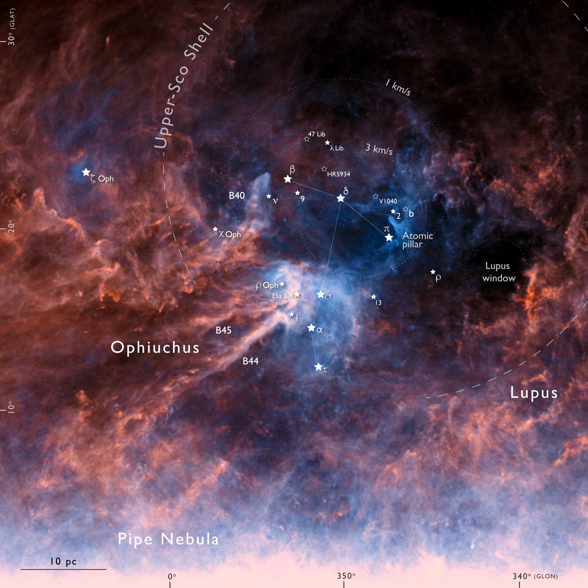
Figure 1: Color composite of the Ophiuchus, Pipe Nebula, and Lupus cloud complexes (blue: extrapolated Planck 250 $\mu$m, green: Planck 350 $\mu$m, red: Planck 500 $\mu$m). Star symbols represent the position of massive ionizing stars (B3 or earlier), while symbol size represents relative brightness. Most of these stars have associated H${\alpha}$ extended emission, while only the two fainter objects are not associated with WISE extended emission. Most, if not all stars in this Figure are interacting with the molecular cloud complex and constitute the main source of dust heating (the bluer regions) in the complex.

Filamentary structures are now established as the predominant morphology of the projected gas density field in the ISM, in both atomic and molecular forms (e.g., Hacar et al., 2023; Pineda et al., 2023). ISM filaments span a wide range of sizes, from kpc-long filaments (e.g., Zucker et al., 2017) to sub-pc-length (e.g., Hacar et al., 2018). Although the term “filament” can refer to thread-like structures across various astronomical contexts, we adopt its common ISM definition: projected cloud structures with aspect ratios greater than three. The underlying mechanisms driving the formation of filamentary gas clouds remain the subject of debate and research. Several hypotheses have been proposed. Potential processes responsible for or contributing to filament formation include sheet-like structures seen edge-on, instabilities in such sheets, dynamics of colliding flows, gravitational forces, effects of shocks, the decay of turbulence, feedback, and the magnetic field (e.g., Nagai et al., 1998; Padoan et al., 2001; Burkert & Hartmann, 2004; Myers, 2009; Peretto et al., 2012; Heitsch, 2013; Hennebelle, 2013; Inutsuka et al., 2015; Tritsis & Tassis, 2018; Arzoumanian et al., 2018; Bonne et al., 2020; Jeffreson et al., 2020; Smith et al., 2020; Pillsworth & Pudritz, 2024).

Molecular clouds may retain imprints of their formation history. These “birthmarks” could manifest as distinct observational signatures, allowing observers to test formation scenarios. To investigate this possibility, we need wide-field, high-dynamic range maps of entire cloud complexes. Such maps would enable us to study not only the dense star-forming regions, but also the surrounding diffuse gas that provides crucial context for a cloud’s origin. In this paper, we search for such “birthmarks” within the filamentary structures of the Ophiuchus molecular cloud complex. Our analysis uses observations from Herschel, Planck, and 2MASS, providing a comprehensive view of the cloud across a wide range of densities and temperatures.

2 The Ophiuchus complex

The Ophiuchus complex is not an isolated star-forming region, but rather a component of the nearby Sco-Cen OB association, a region that has formed about 13000 stars in the last $20\text{\,}\mathrm{M}\mathrm{y}\mathrm{r}$. Most of these stars were formed 15 Myr ago, at the peak of this region star formation rate (Ratzenböck et al., 2023b). The OB association also includes the cloud complexes of Lupus, the Pipe Nebula, L134, Corona Australis, and Chameleon. These regions, once thought to be distinct, are now understood to represent the remnants of a larger, single star-forming region (Bouy & Alves, 2015; Ratzenböck et al., 2023b). The Ophiuchus complex is embedded within Upper-Sco, a sub-region of Sco-Cen that still harbors approximately 20 massive ionizing stars (e.g., Miret-Roig et al., 2022) and started to form about 10 Myr ago.

A Galactic bubble residing at the boundary between the halo and the Galactic disk in Upper-Sco was identified by Robitaille et al. (2018). This suggests a supernova explosion occurred 1–$3\text{\,}\mathrm{M}\mathrm{y}\mathrm{r}$ ago, with the resulting shock wave expanding into a pre-existing HI loop created by outflows from the Upper-Sco region. Robitaille et al. (2018) propose that this supernova feedback event triggered the formation of the Ophiuchus and Lupus molecular clouds. Further supporting this scenario, Neuhäuser et al. (2019) found kinematic evidence that the runaway star $\zeta$-Oph and the radio pulsar PSR B1706-16 were ejected from a binary system by a supernova within Upper-Sco approximately $1.8\text{\,}\mathrm{M}\mathrm{y}\mathrm{r}$ ago.

Recently, Piecka et al. (2024) used ISM optical absorption lines to present evidence for a significant Sco-Cen outflow. The outflow has at least two components: a faster, low-density component traced by Ca II, and a slower, possibly lower-density component traced by Mg II and Fe II. The average radial velocity of this outflow is about -21 km/s and it correlates, partly, with HI emission. A faster flow component, without HI gas, is traceable only in the Ca II line. A flow model suggests an extended distribution of feedback sources within Sco-Cen.

The Ophiuchus region is one of the closest star-forming complexes to Earth (e.g., de Geus, 1992; Lombardi et al., 2008; Loinard et al., 2008; Schlafly et al., 2014; Zucker et al., 2020), and, historically, has served as a crucial laboratory to advance our understanding of star formation (e.g., Struve & Rudkjobing, 1948; Blaauw, 1964; Montmerle et al., 1983; Lada & Wilking, 1984; Loren, 1989a; Ward-Thompson et al., 1994; Andre & Montmerle, 1994; Tachihara et al., 2000b, 2001); see Wilking et al. (2008) for a review. This complex exhibits a wealth of filamentary gas structures, mostly cataloged Lynds clouds (Lynds, 1962) (see Figure 2, and can be broadly divided into three subregions:

1. Ophiuchus Classic: This region encompasses the L1688 clump (also known as the $\rho$ Oph core), which contains the closest embedded star cluster to Earth, along with the B44 and B45 filaments. These filaments host the actively star-forming regions L1689 (e.g., Nutter et al., 2006) and L1709.

2. Oph North: A filament complex characterized by prominent cores that show limited signs of active star formation (Hatchell et al., 2012).

3. B40: A less dense and less studied region, also known as the blue horse nebula (illuminated by $\nu$-Sco), including the less known Lynds clouds L1719, L1757, L1782.

Distance estimates to Ophiuchus vary, with Lombardi et al. (2008) reporting $119\text{\,}\mathrm{p}\mathrm{c}$ and Ortiz-León et al. (2017) reporting $137\text{\,}\mathrm{p}\mathrm{c}$ and $147\text{\,}\mathrm{p}\mathrm{c}$ for L1688 and L1689 (the head of B44), respectively, probably reflecting the 3D structure of the complex. Recent work by Zucker et al. (2019, 2020) found distances ranging from $118\text{\,}\mathrm{p}\mathrm{c}$ to $149\text{\,}\mathrm{p}\mathrm{c}$ towards the $\rho$ Oph region (L1688) and the Ophiuchus streamers (B44 and B45), with an average distance of $139\text{\,}\mathrm{p}\mathrm{c}$. For simplicity, we adopt an average distance of $140\text{\,}\mathrm{p}\mathrm{c}$ throughout this paper. At this distance, Herschel dust emission maps achieve resolutions of approximately $4000\text{\,}\mathrm{A}\mathrm{U}$ ($0.02\text{\,}\mathrm{p}\mathrm{c}$) at $500\text{\,}\mathrm{\SIUnitSymbolMicro}\mathrm{m}$ and $2000\text{\,}\mathrm{A}\mathrm{U}$ ($0.01\text{\,}\mathrm{p}\mathrm{c}$) at $250\text{\,}\mathrm{\SIUnitSymbolMicro}\mathrm{m}$.

In this paper, we analyze the 2D column density map of the Ophiuchus region, created using data from the Herschel, Planck, and 2MASS surveys (referred to as HP2), as well as the distribution of massive ionizing stars. Our goal is to uncover signs of the process, or processes, that lead to the formation of filaments in this region. We search for these signs by examining the distribution of mass within the Ophiuchus complex and exploring any potential connections between the arrangement of gas and the presence of massive stars in the region. We find evidence that stellar feedback from massive stars in Upper-Sco played a crucial role in shaping the gas complex in Ophiuchus. This influence extends to the ongoing star formation activity within the association, namely the Lupus cloud complex and the Pipe Nebula.

3 Data

The Ophiuchus molecular cloud complex was observed by the all-sky Planck observatory and by two Herschel Space Observatory programs, namely, 1) the Gould Belt Survey (André et al., 2010) covering 26.4 sq deg of the complex including L1688, B44 (L1712) and B45 (L1755), and 2) as part of an Herschel open time program (PI J. Hatchell), covering 24.2 sq deg towards the Northern regions of the complex (part of B40 and L204). For Planck, the 2013 data products were used (Ade et al., 2014). For Herschel, we used 160 $\mu$m observations taken in parallel mode using the PACS instrument (Poglitsch et al., 2010), and 250, 350, and 500 $\mu$m observations using the SPIRE instrument (Griffin et al., 2010). Table 3 presents a log of the Herschel data used in this paper. The data were pre-processed using the Herschel Interactive Processing Environment (HIPE Ott, 2010) version 10.0.2843. A list of the Herschel data used in this paper is given in Table 3.

We follow the general procedure introduced in Lombardi et al. (2014) to derive optical depth and temperature maps for the Ophiuchus complex. The procedure can be summarized as follows: 1) We produce an extinction map of the complex using data from the 2MASS-PSC (Skrutskie et al., 2006; Lombardi et al., 2011) archive and perform a standard reduction of the Herschel data with the HIPE; 2) We then convolve the Herschel images and re-grid them to match Planck’s resolution and data projection; 3) We perform a linear fit between the Herschel and Planck fluxes at the same passband, confirm the linearity between the two, and we applied the proper calibration offset for each individual Herschel passband; 4) We apply the offset to the Herschel images and convolve them to the same resolution (normally the resolution of the SPIRE 500 $\mu$m data); 5) We perform an SED fit pixel-by-pixel using a modified black-body as a model, leaving the optical-depth and dust effective temperature as free parameters; the local value of the spectral index $\beta$ is taken from a Planck/IRAS fit; 6) Finally, we also build a higher resolution map from the SPIRE 250 $\mu$m band by inferring the optical-depth from the observed flux (and assuming $\beta$ from the Planck and $T$ from the 36^′′ resolution SED fit).

4 Results

In Figure 1 we present a $\sim 30^{\circ}\times 30^{\circ}$ square degree color Planck-based composite of the Ophiuchus, Pipe Nebula, and Lupus cloud complexes (blue: extrapolated Planck 250 $\mu$m, green: Planck 350 $\mu$m, red: Planck 500 $\mu$m). The color in this Planck figure corresponds to line-of-sight density weighted temperature (a rough approximation of the true temperature map presented in Figure 3) and ranges from about 10 K (orange) to about 30 K (blue). Star symbols represent the most massive and ionizing stars in the region (spectral type B3 or earlier) and are listed in Table 2. Filled star symbols represent stars with extended emission in WISE images, suggesting a close vicinity and interaction with the complex, while open symbols represent stars without recognizable extended WISE emission (see discussion in A).

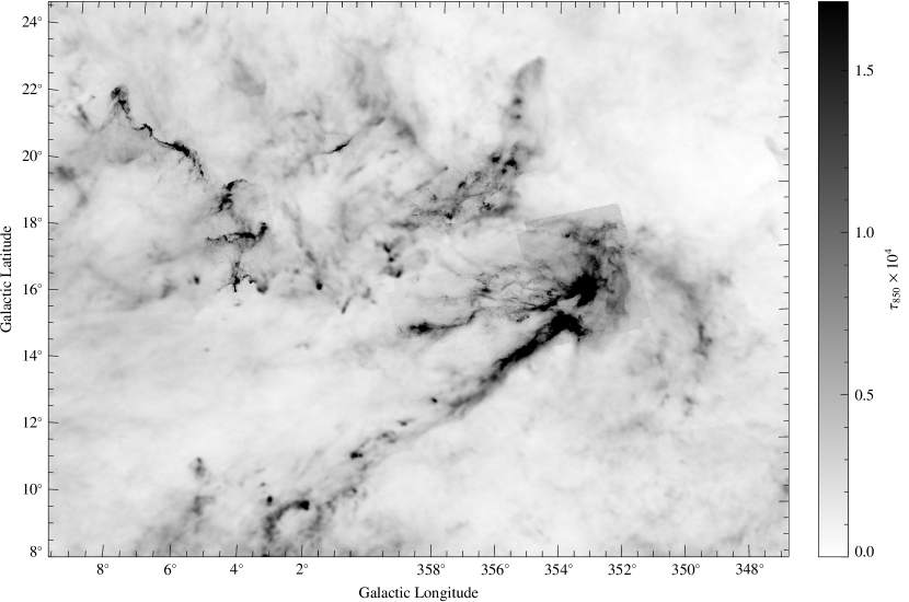
Figure 2: Planck-Herschel optical-depth map for Ophiuchus. The resolution of the map is 5 arcmin (for the Planck data) and 36 arcsec (for the high column density, Herschel-covered areas). The corresponding error map is presented in Figure 15

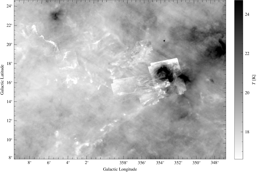
Figure 3: Effective dust-temperature map for the Ophiuchus field. The cold structures appear white, while the higher temperatures appear as black. There are at least seven hot spots, all associated with massive ionizing stars in the region, implying a distance similar to the cloud material they are warming up. Note, by comparison with Figure 2, that most of the hot spots are associated with low column-density regions, the $\rho$ Oph shell being a particularly good example. The corresponding error map is presented in Figure 16

The interplay between massive ionizing stars and interstellar dust in Figure 1 is mesmerizing. The color scheme, representing temperatures ranging from about 10 K (in orange) to 30 K (in blue), enables a detailed view of the relationship between radiation from young massive stars and the distribution of warm dust across the star-forming complex. The figure labels the major cloud complexes and notable structures such as the B44 and B45 “streamers” and the poorly studied B40 structure (Nozawa et al., 1991). The thin solid lines trace stars in the Scorpius constellation, aiding orientation. The Upper-Sco shell (de Geus, 1992) is indicated by a large dashed circle. A new pillar-like structure near $\pi$ Sco, not detected in the ¹²CO survey by Tachihara et al. (2001) but observed in the HI survey by Kalberla & Haud (2015), is also highlighted and labeled “Atomic Pillar”. The existence of a low column-density area, the “Lupus window,” near the Lupus 1 cloud (Franco, 2002), is confirmed. This figure illustrates the complex interplay between a previous generation of massive stars and star-forming clouds, showing a correlation between heating and gas distribution over tens of parsecs. It highlights the importance of taking into account the wider context of a star-forming complex, rather than concentrating exclusively on particular subregions.

4.1 Column density and temperature maps

In Figure 2 we present the Planck-Herschel optical-depth map for the Ophiuchus field constructed using the method described in Lombardi et al. (2014). The map covers approximately 380 square degrees of the sky ($22.5^{\circ}\times 17^{\circ}$) or about $50\times 35$ pc² at the distance of the complex. The map has a dynamic range that spans about 3 orders of magnitude, from about $A_{\rm V}\sim 0.3$ mag (10$\sigma$) to $A_{\rm V}\sim 300$ mag, or about $6\times 10^{20}$ to $6\times 10^{23}$cm^-2. This large dynamic range can be reached due to the hybrid approach followed in Lombardi et al. (2014) which combines the higher resolution Herschel data with the very low noise Planck data. The mean and median column density values on the map are about $A_{\rm V}\sim 1.4$ mag.

In Figure 3 we present the effective dust temperature map for the combined Herschel and Planck maps of the Ophiuchus field. The minimum, mean, and maximum temperature on this map are about 11, 19, and 36 K. The temperature maxima in the map coincide with the location of well known ionizing stars, namely the runaway O-star $\zeta$ Oph to the East, $\rho$ Oph (defining an almost circular shell), $\sigma$ Sco, and $\pi$ Sco, which is close to, and likely interacting with, the Atomic pillar structure seen as diffuse blue light in the optical, and as warm dust (about 30 K) in Figure 1.

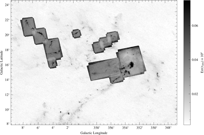
Figure 15: Error map for the optical-depth for the map reported in Figure 2. The figure shows the areas where the Herschel data are available (higher errors). The resolution of the image varies from 5 arcmin (for the Planck data, low error region) to 36 arcsec (for the Herschel, higher error region).

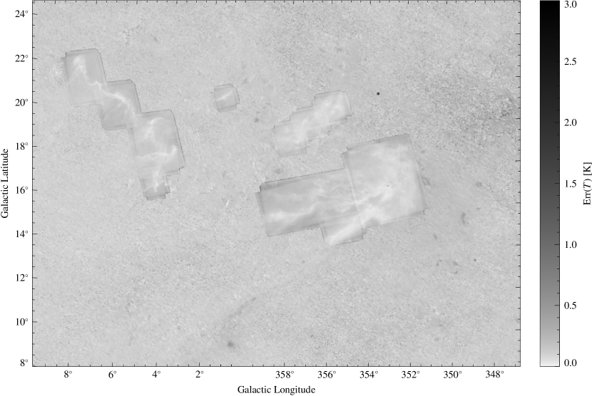
Figure 16: Error map for the effective dust-temperature map reported in Figure 3.

The combined Herschel and Planck maps (Figure 2 and 3) provide coverage of the Ophiuchus complex at two different resolutions: 36^′′ for the high column density regions covered by Herschel, and 5^′ for the lower density regions covered only by Planck. Although the seams between these datasets are generally imperceptible, they become apparent in the L1688 field, which exhibits the highest luminosity. These seams are easily visible on the column density and temperature error maps (Figures 15 and 16).

In Figure 4, we present the Meisner & Finkbeiner (2014) temperature map of the Ophiuchus-Lupus-Pipe region. Meisner & Finkbeiner (2014) applied the Finkbeiner et al. (1999) two-component thermal dust emission model to Planck HFI maps for a better fit of the far-infrared dust spectrum and demonstrated that their approach provides more accurate predictions in diffuse sky regions compared to the single-MBB model used by the Ade et al. (2013) Planck Collaboration map. The darker grayscales in this figure represent colder temperatures. Compared to the emission map in Figure 1, the temperature map provides a better separation between the nearby cold complexes that we want to study and the unrelated background of dust clouds. This is best seen for complexes closer to the Galactic plane, like the Pipe Nebula and some of the Lupus clouds, where the contrast between the nearby cold cloud and the warmer unrelated material along the same line-of-sight is highest.

Table 1: Derived masses for cloud structures in Ophiuchus from the HP2 map (Fig. 2)

Name	Area	$\langle A_{\rm{K}}\rangle$	Mass	Surf. Density
	pc2	mag	M⊙	M${}_{\odot}/\rm{pc}^{2}$
Entire HP2 map	2405.9	0.2	72660	30
$A_{{\rm K}}>0.1$	2004.9	0.2	67048	33
$A_{{\rm K}}>0.5$	34.9	0.9	5196	149
$A_{{\rm K}}>0.8$	10.0	1.6	2660	267
L1688 $A_{\rm{K}}>0.5$	5.7	1.4	1367	242
L1688 $A_{\rm{K}}>0.8$	2.9	2.2	1081	374
L1689 $A_{\rm{K}}>0.5$	4.2	1.1	780	188
L1689 $A_{\rm{K}}>0.8$	2.2	1.5	563	261
B44 $A_{\rm{K}}>0.5$	9.9	0.9	1485	150
B44 $A_{\rm{K}}>0.8$	6.6	1.0	1123	170
L1712 $A_{\rm{K}}>0.5$	3.3	0.8	465	140
L1712 $A_{\rm{K}}>0.8$	1.3	1.1	250	187
B45 $A_{\rm{K}}>0.5$	2.4	0.8	345	141
B45 $A_{\rm{K}}>0.8$	0.7	1.3	147	227
L1709 $A_{\rm{K}}>0.5$	1.2	1.0	206	170
L1709 $A_{\rm{K}}>0.8$	0.5	1.6	129	279
L43 $A_{\rm{K}}>0.5$	0.3	1.2	52	203
L43 $A_{\rm{K}}>0.8$	0.2	1.5	45	251
Oph N $A_{\rm{K}}>0.5$	5.8	0.5	495	85
Oph N $A_{\rm{K}}>0.8$	1.7	1.3	374	223
Oph Arc	71.9	0.2	2675	37
B40	78.0	0.3	3569	46
Atomic Pillar	3.1	0.1	55	17

4.2 Masses

In this section, we estimate the gas masses for the Ophiuchus field (Figure 2), and for individual subregions, as a function of a column-density threshold. To derive masses from the column density map presented in Figure 2 we integrate the column density over an area of interest in the cloud (as in, e.g., Lombardi et al., 2014; Zari et al., 2016). In Table 1 we present the masses for well-known structures in Ophiuchus, including two distinct column density thresholds ($A_{\rm K}>0.5$ and $A_{\rm K}>0.8$) mag. The former was chosen to separate the main structures as lower thresholds would merge the main structures. The latter threshold is associated with star formation activity (Lada et al., 2010) and most of the gas above this threshold is part of only three star-forming gas structures, namely, L1688, B44, and B45. Note that L1689 and L1712, and L1709 are part of the B44 and B45 structures, respectively (see Fig. 2). We associate L1719, L1757, and L1782 with B40 to calculate the mass of this structure. We compare our masses estimates to the CO-derived masses in Loren (1989a), de Geus & Burton (1991), and the Herschel-derived masses in Howard et al. (2021) using a different approach to ours. On average, our masses are about 40% higher than the CO-derived masses. This suggests that dust emission appears to capture a factor of 1.4 times more mass than CO. Our masses are about 10% higher than the alternative Herschel-derived masses. Given the uncertainties in the definitions of the cloud boundary, in particular for the CO work, the differences might not be substantial.

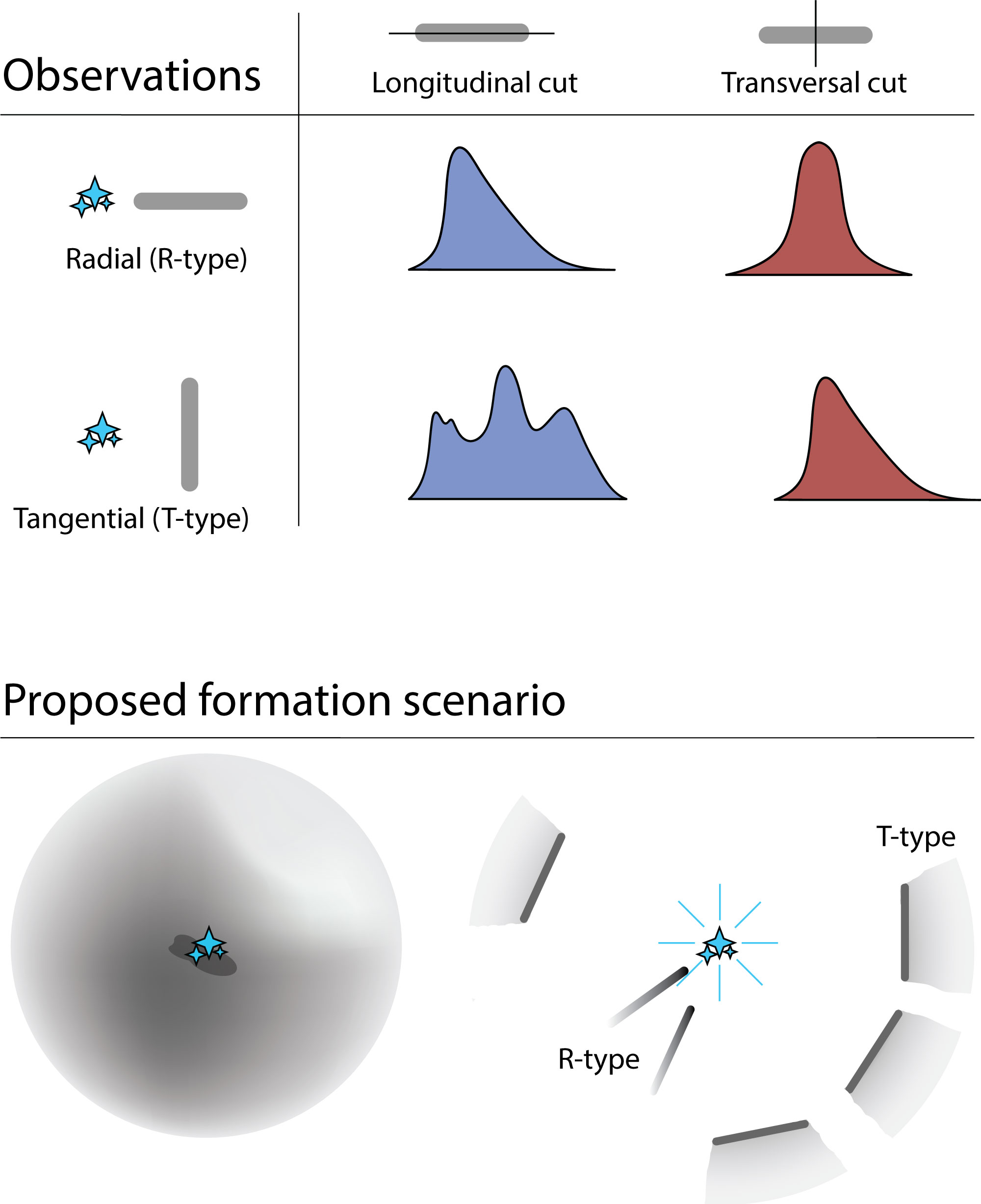
Figure 10: Top: Summary of the longitudinal/transversal profile analysis. R-type profiles exhibit asymmetric longitudinal profiles and symmetric transversal profiles, whereas T-type profiles are characterized by generally flatter longitudinal profiles and asymmetric transversal profiles. These pronounced distinctions between the two filament types imply the existence of two separate mass assembly mechanisms. Bottom: A schematic representation of the proposed formation scenario. Variations in the initial gas distribution following the formation of massive stars may account for the emergence of the two filament types. T-type filaments could arise from a shell fragmentation process, while R-type filaments may result from the stretching and compression of denser gas in proximity to newly formed massive stars.

We estimate the mass of the entire complex from the Planck map in Figure 4 to be about $1\times 10^{5}$ M_⊙. The total Sco-Cen gas is about $2\times 10^{5}$ M_⊙, which means that half of the gas is currently associated with Upper-Sco. To estimate the total mass, we integrated the Meisner & Finkbeiner (2014) column density map over the area covered by the entire OB association (about $220\times 150$ pc², see Figure 10 of Ratzenböck et al., 2023b) and subtracted an equal area, equal Galactic longitude, control field taken west of Sco-Cen. We avoided a band of $\pm{3}$ degrees centered on the Galactic plane, where confusion is extreme.

4.3 Orientation and surface density profile of filaments in complexes surrounding Upper-Sco from Planck data

The overall morphology of the region, illustrated in Figure 4, including its warmer interior surrounded by colder dense gas arranged in a non-random filament orientations, reveals the influence of feedback from Sco-Cen OB stars. To investigate this potential influence, we analyzed the orientations of the filamentary structures shown in Figure 4. We began by estimating the center of Upper-Sco using the distribution of warm dust — displayed as black (around 13 K) to white regions (around 20 K) in Figure 4 — as a tracer of the combined effects of massive stars on the surrounding material. The region of peak temperature aligns with the estimated location of the most recent supernova in Upper-Sco (Neuhäuser et al., 2019), and we therefore adopt this supernova’s location ($l=-13^{\circ}$, $b=21^{\circ}$) as the working center of Upper-Sco.

To determine the orientation of each filament, we measured the angle between two lines: a) the line connecting the adopted center of Upper-Sco to the midpoint of the filament, and (b) the filament’s long axis. Figure 5 displays the resulting distribution of filament orientations. Given the improbable assumption that there is a single source of feedback, the distribution exhibits nevertheless two preferred orientations: radial and tangential, with peaks near $0^{\circ}$ and $80^{\circ}$, respectively. A Kolmogorov–Smirnov (KS) test confirms that this bimodal distribution is unlikely to occur by chance when compared to a flat distribution ($p=0.03$).

This result is particularly noteworthy because we used a single center for all filaments, which probably does not accurately represent all feedback sources in the region. For example, L204 in Oph North is tangential to, and likely influenced by, the runaway O-star $\zeta$ Oph, located approximately $20^{\circ}$ away from our adopted center. In this analysis of filament orientation, we focused on the main filamentary structures seen in Figure 4, many well-studied molecular clouds. We avoided regions of confusion, without a clear filamentary structure, like B40. Still, many more filamentary structures can be seen through out the map following the general trend of the main filaments.

We constructed column density profiles for the filaments shown in Figure 4 using longitudinal (along the filament) and transversal (across the filament) cuts on the Planck column density map derived by Meisner & Finkbeiner (2014). Figure 6 illustrates examples of these column density profiles for radial filaments (from hereafter, R-type), shown in blue. R-type filaments exhibit asymmetric longitudinal profiles, with their heads oriented towards massive stars. In the larger Upper-Sco region, this pattern holds not only for major Ophiuchus filaments but also for the Pipe Nebula stem and smaller, less-studied filaments. However, the transversal column density profiles of R-type filaments, shown in red, differ significantly, showing approximate symmetry.

Figure 7 presents the equivalent analysis for tangential filaments (from hereafter, T-type). T-type longitudinal column density profiles tend to have multiple peaks, contrasting with R-types. Furthermore, T-types lack the distinct longitudinal asymmetry (“head-tail” morphology) characteristic of R-type filaments. However, T-type transversal column density profiles are asymmetric, resembling the longitudinal profiles of R-type filaments.

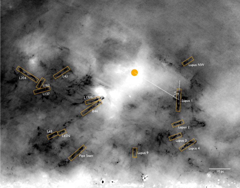
Figure 4: Orientations of the main filaments (enclosed in the orange boxes) in the Ophiuchus-Lupus-Pipe region, shown on the Meisner & Finkbeiner (2014) temperature map. The orientation angles were measured between the filament axis and the direction to a central point near the peak of the temperature map, marked with a closed orange circle in the map. This point is consistent with the location of the last supernova in Upper Sco (about 2 Myr ago, Neuhäuser et al. 2019).

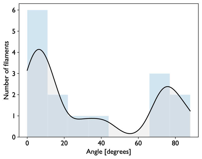
Figure 5: Distribution of filament orientations in the Upper-Sco region as shown in Figure 4.

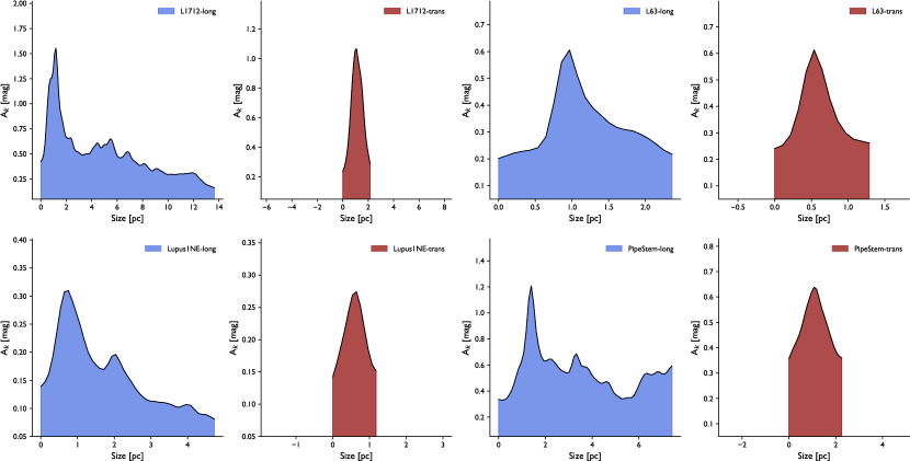
Figure 6: Selected examples of R-type longitudinal (blue) and latitudinal (red) mass profiles. An observable pattern emerges, specifically, R-type filaments predominantly exhibit asymmetric longitudinal distributions (head-tail configuration) and symmetric transverse distributions.

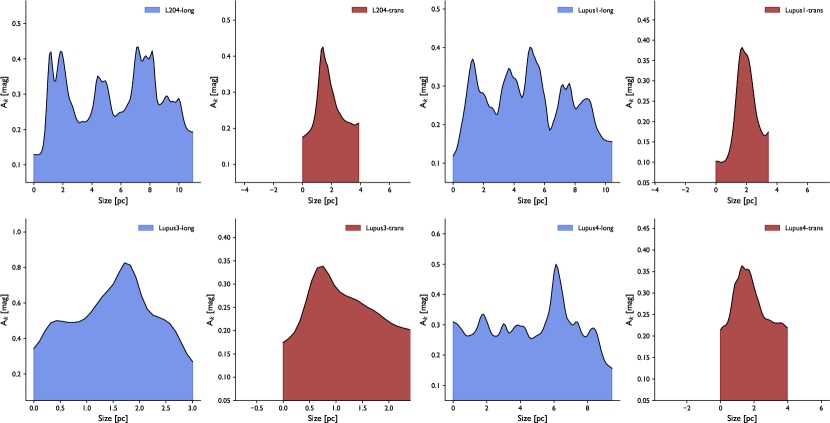
Figure 7: Selected examples of T-type longitudinal (blue) and transversal (red) column density profiles. In contrast to R-type filaments, T-type filaments do not exhibit head-tail morphology. Their longitudinal profiles are generally flat, with dense cores and star formation distributed along their length and no significant mass accumulation toward either end. Interestingly, their transversal profiles often display asymmetry, suggesting mass “spillover” on the side facing away from the feedback flow. This asymmetry is another distinguishing feature compared to R-type filaments.

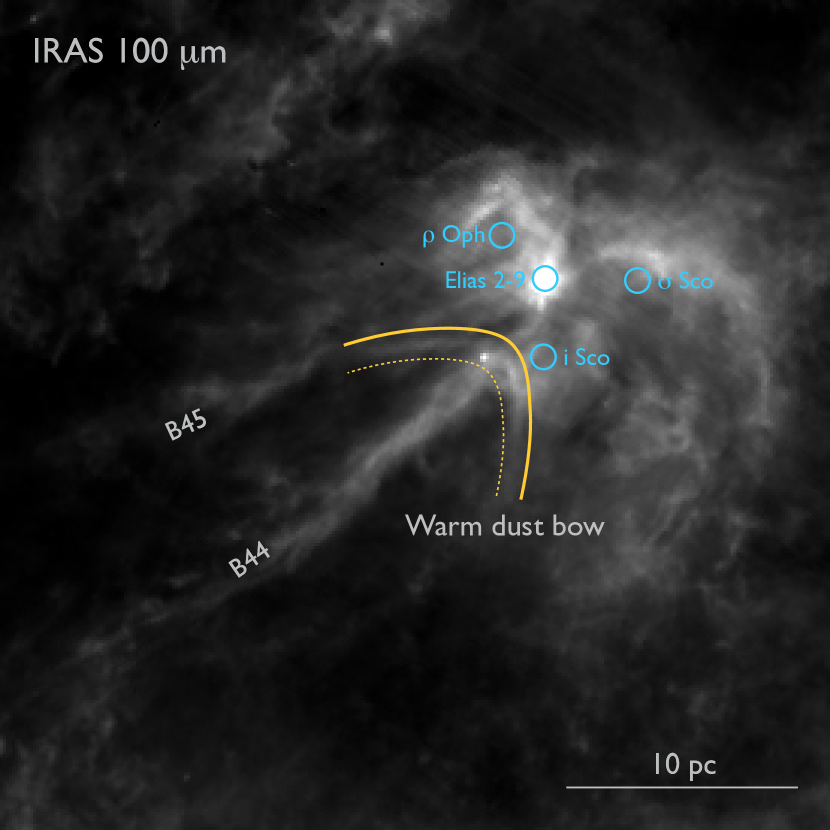
Figure 8: IRAS 100 $\mu$m image of the Ophiuchus region. The image reveals a bow-like dust feature at the head of B44, suggestive of a bow-shock. If a bow-shock, the Mach number of the flow interacting with B44 is about 2.

4.4 Further evidence for feedback-driven environment from Herschel data

In this section, we present evidence that feedback from massive stars in Upper-Sco affects the mass distribution of filamentary clouds in Ophiuchus. Although each piece of evidence alone is not definitive, they collectively support this scenario. Several features visible in Figure 12 imply a direct influence from massive stars:

• Filamentary structures appear wind-blown, extending away from the massive stars in Upper-Sco (see also Figure 1)

• The B44 and B45 filaments align approximately radially with the massive stars in Upper-Sco, including $\sigma$ Sco, Elias 2-9 (HD147889), and $\delta$ Sco

• Present-day star formation, traced by Class I protostars, occurs within L1688 and at the tips of B44, B45, and L1709 facing the massive stars

• The linear arrangement of Class I protostars in L1688 is orthogonal to the line connecting L1688 and $\sigma$ Sco, suggesting a compressive shock

Below, we present complementary evidence for direct interaction between a feedback flow and the gas distribution.

4.4.1 Bow-shock feature

Figure 8 shows the IRAS 100 $\mu$m image of Ophiuchus, highlighting L1688, B44, B45, and key massive stars. A prominent bow-shaped feature, the “Warm Dust Bow,” appears near B44. Faintly detected in Herschel data, it likely represents warmer dust. We suggest this is a bow shock formed by interaction between gas at B44’s leading edge and winds from massive stars in Upper-Sco, particularly Elias 2-9 (HD147889).

If this interpretation is correct, the bow shock’s shape provides an estimate of the Mach number $M$. The Mach angle $\theta\approx 35^{\circ}$ implies $M=1/\sin(\theta)\approx 2$ (e.g., Landau & Lifshitz, 1987; Shore, 2007), indicating a supersonic flow interacting with B44. The shapes of the Oph Arc (near $\sigma$ Sco) and the $\rho$ Oph shell are also consistent with a flow arriving from the northwest, originating near the ionizing stars in Upper-Sco.

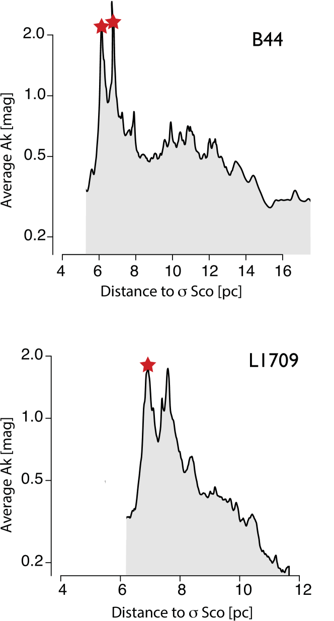
Figure 9: Longitudinal mass profiles of Ophiuchus’s densest R-type filaments (B44 and L1709 at B45’s head) at Herschel’s higher resolution. As in the lower resolution Planck-based profile in Figure 6, the linear mass density decreases from the head, closest to the massive stars, towards the tail. Class I protostars, tracers of ongoing star formation, are shown as red stars and associated with the maxima of the profile.

4.4.2 R-type profiles at high resolution

Figure 9 shows longitudinal Herschel column-density profiles of B44, L1709 (at the head of B45), with Class I protostars marked as red stars. These are higher resolution versions of the Planck-based R-type profiles presented in Figure 6. The filament’s linear mass density decreases from its maximum closer to the massive stars to its minimum downstream from these luminous stars, at the opposite end of the filament. Star formation is occurring only at the maxima of the profile, towards the end of the filament facing the massive stars. The location of ongoing star formation and the filament mass gradient are hard to explain without an interaction between dense gas and a stellar feedback flow.

4.4.3 The 3D motion of the Ophiuchus complex

Stellar feedback influencing Ophiuchus would imply that it moves away from Upper-Sco’s massive stars under ram pressure. Because most massive stars lie above Ophiuchus, we expect the clouds to move downward if feedback is at play. If Ophiuchus moved upward instead, this would contradict the feedback scenario.

Grasser et al. (2021) analyzed Gaia EDR3 data to determine the 3D motion of young stellar objects (YSOs) in Ophiuchus, primarily around L1688. These YSOs, still forming and optically visible, trace the gas motion. They find $UVW=(-5.2\pm 4.1,-15.1\pm 1.2,-9.3\pm 1.6)\,\textrm{km/s}$, differing from Upper-Sco’s $UVW=(-5,-16,-7)\,\textrm{km/s}$ (Luhman & Esplin, 2020). The velocity difference is $\Delta_{UVW}=(0,0.9,-2)\,\textrm{km/s}$, implying Ophiuchus moves away, mostly downward, from Upper-Sco’s massive stars. This motion supports, but does not prove, the feedback scenario. It also agrees with the ground-based results by Ducourant et al. (2017), who find $UVW=(-5.9\pm 0.1,-14.2\pm 0.3,-8.1\pm 0.4)\,\textrm{km/s}$.

Ratzenböck et al. (2023b, a) identified that massive stars such as $\sigma$ Sco and $\delta$ Sco, without Gaia parallaxes due to saturation, lie near the centers of newly identified Gaia clusters. They likely share similar 3D motions with their clusters. Traceback studies by Miret-Roig et al. (2022) show that the $\rho$ Oph cluster was within $1\text{\,}\mathrm{p}\mathrm{c}$ of $\delta$ Sco about $5\text{\times}{10}^{6}\text{\,}\mathrm{y}\mathrm{r}$ ago. This close past interaction suggests that $\delta$ Sco and other massive stars have influenced the Ophiuchus cloud’s morphology and dynamics.

5 Discussion

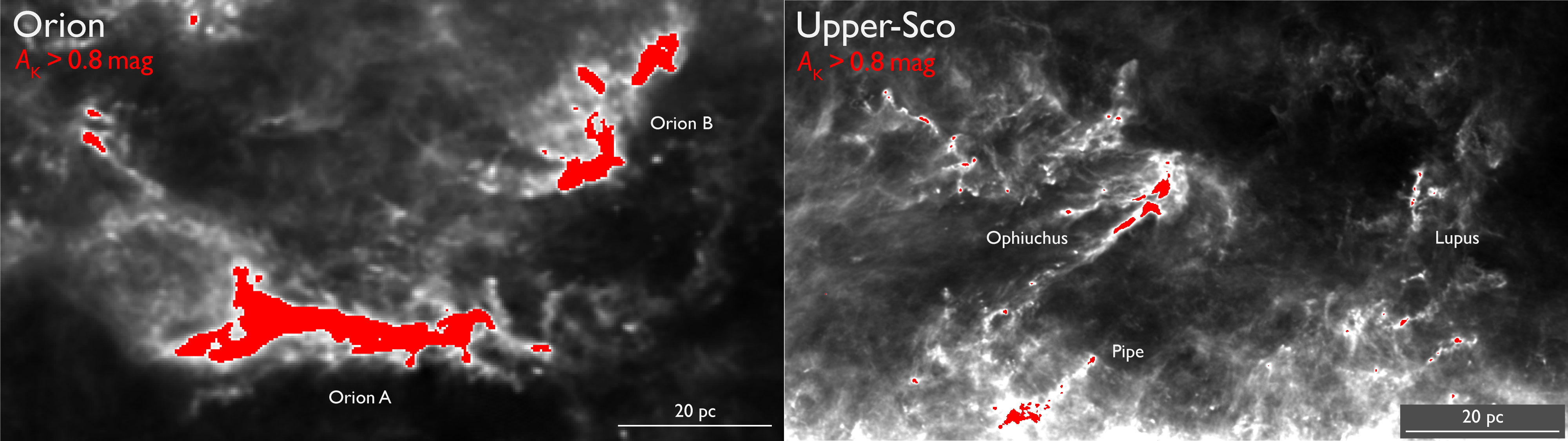
Figure 11: Comparing the Orion and Upper-Sco complexes at the same physical scale reveals striking differences in the amount and distribution of dense gas. The greyscale represents the Planck column-density map (Meisner & Finkbeiner, 2014), and red marks regions with dense gas ($A_{K}>0.8$ mag) likely to collapse into new stars. While the gas mass in Orion is about twice that of Upper-Sco, Orion contains ten times more dense gas. Critically, dense gas in Orion is concentrated in two main filamentary clouds, whereas Upper-Sco’s dense gas is more scattered across the region.

The arguments presented earlier, and numerous previous studies, support the idea that the feedback from massive stars in Upper-Sco plays a crucial role in shaping the region, aligning with previous studies (e.g., Vrba, 1977; Loren & Wootten, 1986; Loren, 1989a; de Geus, 1992; Onishi et al., 1999; Tachihara et al., 2000b, a; Preibisch & Mamajek, 2008; Peretto et al., 2012; Krause et al., 2018; Robitaille et al., 2018; Ladjelate et al., 2020). Furthermore, because of the superior sensitivity and dynamic range of Planck and Herschel, we found revealing patterns, birthmarks, in the alignment of dense gas filaments, their column density profiles, and the locations of star formation activity. All the evidence presented here points to a formation mechanism that organizes gas and star formation in clear patterns over at least 60 pc regions. Following the evidence, we suggest that the feedback flow from massive stars in Upper-Sco is the primary force driving the formation of most filamentary structures in the region.

The scenario presented here relies on the presence of a significant outflow of diffuse gas from the Sco-Cen association. Until recently, evidence for the existence of such a flow was scarce (Hobbs, 1969; Frisch & York, 1986). This flow was recently reported through ISM absorption lines in this region (Piecka et al., 2024). The outflow has a radial velocity of approximately $-21$ km/s and is generally correlated with the HI emission. Likely driven by stellar feedback from massive stars in Sco-Cen, the outflow exhibits a complex structure, including a faster component identified through Ca II absorption only. This high-velocity component suggests a dynamic and energetic outflow capable of influencing the surrounding interstellar medium, including the Ophiuchus complex.

5.1 Creation through destruction: the origin of R-type and T-type filaments

The simplest model that seems to fit the observations discussed here is one in which a feedback flow from the newly born massive stars towards the center of Upper-Sco rearranges the leftover gas into radial and tangential filaments. An explanation for this bimodal outcome is probably rooted in the initial conditions of the leftover gas. We present two possible formation scenarios below:

• R-type filaments: The flow will quickly disperse the less dense gas leaving behind pockets of compressed denser gas. These will act as a resilient shield against the flow that creates stagnation points, like rocks in a stream (e.g., Padoan et al., 2001; Rogers & Pittard, 2013; Zamora-Avilés et al., 2019b). These dense pockets will cast a radial protective “shadow” against the ram pressure of the feedback flow and will naturally develop into head-tail filamentary radial structures (e.g., Gritschneder et al., 2010; Mackey & Lim, 2010), or R-type filaments with asymmetric longitudinal column density profiles and symmetric transversal profiles (Figure 6). Unsurprisingly, star formation will mostly take place at these densest regions of the R-type filaments (their heads) and good examples are L1688 ($\rho$-Oph core), L1689, L1709, and B59 in the Pipe Nebula.

  An interesting test of this scenario would be to measure the 3D gas flow of any streaming motion along a filament. Although gas kinematic measurements are readily obtained, demonstration of any streaming motion would require knowledge of the filament 3D orientation. Currently, such a measurement is challenging. However, upcoming 3D dust maps of nearby complexes using Gaia DR4 data may soon enable measurements of the true space orientation of some filaments. And, in combination with kinematic observations, provide the opportunity to test the feedback-driven formation scenario proposed here.

• T-type filaments: The less dense gas, incapable of resisting the ram pressure of the flow, will be pushed outwards and accumulate in a shell at a larger distance from the center. This shell will eventually fragment into filaments that are born tangential to the flow that created them. These tangential filaments, while containing star-forming cores, do not show an obvious gradient in their longitudinal column density profiles (Figure 7). Interestingly, their asymmetric transversal column density profiles, with excess mass on the side away from the center for most cases, suggests a mass “spillover” on the side of the filament opposite the flow (Tachihara et al., 2000a), likely due to a process similar to the formation of the head-tail configuration for R-types. The T-type formation mechanism mostly coincides with the classical collect-and-collapse model of Elmegreen & Lada (1977) (see also Dale et al., 2007; Zamora-Avilés et al., 2019a; Whitworth et al., 2022). Good examples of T-type filaments include L204 (tangential to $\zeta$-Oph), Lupus 1, 2, 3, and 4.

5.2 Timescale considerations

Can the feedback scenario plausibly explain the formation of a 20 pc R-type filament like B44 within a reasonable timescale? In this scenario, the head of B44 acts as a stagnation point of the flow, resisting it, and suffering the highest flow ram pressure. Flow streamlines would then split and divert around the stagnation point, shearing the denser gas, eventually stretching the original gas cloud into a filament. The feedback scenario then implies that the gas along B44 must have originated, mainly, from the filament head.

A key test for evaluating the feedback scenario in Upper-Sco is the age of the massive stars driving the flow. Based on high-resolution star formation histories derived from Gaia data, this age is estimated to be approximately 10 Myr (Ratzenböck et al., 2023a). At first approximation, and for R-type filaments, this suggests an average gas streaming velocity of about 2 km/s within the B44 filament, covering the 20 pc distance from head to tail over 10 Myr. This estimate is consistent with the observed radial velocity of the gas across B44 (Loren, 1989b), though the true 3D orientation of the filament remains unknown, making the actual streaming velocity uncertain.

Determining the 3D orientation of B44 is crucial for accurately measuring gas motion within the filament, a key aspect of the feedback-driven formation scenario. Confirming the presence of such motion could help identify the dominant feedback processes. For example, Robitaille et al. (2018) suggested that both Ophiuchus and Lupus formed as a result of feedback flows triggered by a supernova 1-3 Myr ago. This would imply much higher streaming velocities — on the order of 7-20 km/s — which could be possible depending on the actual 3D orientation of B44.

5.3 A dispersing cloud complex

With the understanding that Sco-Cen forms a single star formation region containing over $10^{5}$ M_⊙ of gas and approximately 13,000 stars formed in the last 20 Myr, we can place our observations in the broader context of giant molecular cloud (GMC) evolution. This new perspective on the Sco-Cen OB association has been enabled by the exquisite data from ESA’s Gaia mission (Gaia Collaboration et al., 2023). Gaia revealed a complex tapestry of overlapping young stellar populations and the three-dimensional distribution of gas in the association (Ratzenböck et al., 2023b, a; Edenhofer et al., 2024), providing new insights into the star formation history of Sco-Cen.

The star formation history of Sco-Cen can be summarized as follows: the zenith of star formation activity occurred approximately 15 Myr ago, when the bulk of the stars in the association were formed. Since then, star formation activity has steadily declined to the relatively low levels observed today in Ophiuchus, Lupus, Pipe Nebula, CrA, Chameleon, and L134 (Ratzenböck et al., 2023a). These well-studied molecular clouds are the remnants of the primordial Sco-Cen GMC and we are currently witnessing the advanced stages of its dispersal.

To contextualize the Sco-Cen GMC’s dispersal, Figure 11 compares the Orion region (Orion A and B clouds) and the Upper Sco region (Ophiuchus, Lupus, and the Pipe Nebula). Both regions are molecular cloud complexes of comparable mass and size, shown here at the same physical scale for direct comparison. In these maps, grayscale shading represents Planck column density data (Meisner & Finkbeiner, 2014), while regions with $A_{K}>0.8$ mag, indicative of dense gas likely to form new stars (Lada et al., 2010), are highlighted in red. The contrast between the amount and spatial distribution of dense gas in Orion and Upper-Sco, as illustrated in Figure 11, is pronounced. Although Orion contains a total gas mass of $2\times 10^{5}$ M_⊙ — about double that of Upper-Sco — it has ten times more dense gas. Additionally, the dense gas in Orion appears as a cohesive structure concentrated within two major filamentary clouds, whereas in Upper-Sco it is scattered and fragmented across the region, associated with various R- and T-type filaments studied in the previous Section.

Why does Orion contain five times more dense gas per unit mass than Upper-Sco? The distribution of dense gas in Upper-Sco within R- and T-type filaments suggests that feedback from Upper-Sco itself has influenced this arrangement. We propose that the observed differences primarily result from massive star feedback, with Upper-Sco having experienced prolonged exposure to feedback forces relative to Orion. Consider that the main sources of feedback in Upper-Sco are up to 10 Myr and within 10-20 pc of the cloud (see Figure 1, while those in a similar proximity to Orion are a few million years old. Figure 11 thus illustrates the contrasting evolutionary stages of two star-forming GMCs: Orion in an earlier stage of dispersal and Upper-Sco in a later stage.

Given the estimated total gas mass in Sco-Cen ($\sim 2\times 10^{5}$ M_⊙, see Section 4.2), the number of Sco-Cen stars ($\sim 13000$, Ratzenböck et al., 2023b), and a mean stellar mass of 0.42 Myr (Kroupa, 2001), we can estimate the star formation efficiency (SFE) of the large Sco-Cen star forming region to be $\sim 2.7\%$ (e.g., Franco et al., 1994). We can also estimate the average Sco-Cen star formation rate (SFR) over the last 20 Myr to be 273 M_⊙/Myr, even if Sco-Cen SFR is far from uniform over the last 20 Myr (see Figure 3 in Ratzenbock et al., 2023). At the average Sco-Cen SFR, we project that star formation will continue until dense gas consumption in a few Million years, suggesting a Sco-Cen GMC dispersal period of $\leq$ 25 Myr. This dispersal time aligns well with recent estimates of GMC lifetimes, generally in the range of 10-30 Myr (Chevance et al., 2022).

5.4 The future of the Ophiuchus complex

We can forecast the future of the Ophiuchus complex, the Upper-Sco gas component containing the largest amount of dense gas in Upper-Sco (see Figure 11). The dense gas in Ophiuchus ($A_{\rm K}>0.8$ mag Lada et al. 2010) measured from the Herschel column density maps (see Section 4.2) has the potential to form approximately 800 solar masses of stars. This assumes that most gas at $A_{\rm K}>0.8$ mag is likely to collapse and form stars at an efficiency of 30% (Alves et al., 2007). This equates to roughly 1900 stars, demonstrating that Ophiuchus remains a fertile region for star formation for the next few Myr, and the most important one in the entire Sco-Cen. The final relative contribution of Ophiuchus to the star formation budget of Sco-Cen is of the order of 10%. This is a simplified estimate, and it does not account for the potential formation of new dense gas from the compression of diffuse gas.

Rather than forming a single cluster or a random distribution of stars, the future stellar population in Ophiuchus is likely to be structured as the dense gas distribution seen in Figure 11. The current configuration of the L1688 core and the main filaments (B44 and B45) resembles the head-tail morphology of the Corona Australis molecular cloud (e.g., Alves et al., 2014), which is now established to form a chain of young clusters (Ratzenböck et al., 2023a). These sequentially aligned clusters exhibit a decreasing age and mass gradient, consistent with a feedback-driven formation scenario (Posch et al., 2023, 2024). The Ophiuchus complex may give rise to the last chain of clusters in Sco-Cen, and be its star formation closing act.

6 Conclusions

We present column density and temperature maps of the entire Ophiuchus cloud complex obtained from Herschel, Planck, and 2MASS/NICEST extinction data to establish a comprehensive view of the gas distribution in the complex and look for potential “birthmarks” of the filament assembly process. The maps have 36^′′ resolution for the regions observed with Herschel, and have a dynamic range for the column density covering 0.03 mag to 30 mag of A_K, or from $6\times 10^{20}$ cm^-2 to $6\times 10^{23}$ cm^-2.

Our primary finding is that stellar feedback from the Upper-Sco region of the Sco-Cen association exerts a dominant influence on the physical structure of gas in the Ophiuchus-Lupus-Pipe region. In this region, we are witnessing close-up of the latter stages of the dispersal of a giant molecular cloud. The feedback, originating from massive stars that began forming approximately 10 Myr ago, shapes the distribution and star formation activity of the leftover gas in the OB association. Specifically, we find that filaments in this region exhibit preferred orientations, tending to align either radially or tangentially with respect to the Upper-Sco massive stars. Furthermore, star formation activity correlates with the spatial distribution of these massive stars.

The results in this paper illustrate a complex phase in molecular cloud evolution with two simultaneous yet contrasting processes: the formation of filaments and stars via the dispersal of residual gas from a previous massive star formation event. The results also indicate that stellar feedback likely shapes filament formation and evolution in star-forming regions undergoing dispersal by massive stars.

The main results of our analysis can be summarized as follows:

1. The filaments within the Ophiuchus-Lupus-Pipe region exhibit preferential orientations, aligning either radially (R-type) or tangentially (T-type) to massive stars in the region. This suggests that massive star feedback has sculpted the molecular gas, shaping the observed filamentary structures. The age of these filaments is constrained by the age of Upper-Sco, implying they are younger than about 10 Myr. High-resolution Herschel data further support this feedback-driven formation scenario.

2. A straightforward scenario, where feedback from the massive stars in Upper-Sco drives a gas flow capable of rearranging and compressing the leftover gas, can, in priciple, explain the observations. Originating from different initial gas distributions, R-type filaments, with star formation at their heads, are likely the remants of denser gas clouds compressed and stretched into filaments, while T-type filaments are the result of a classical collect-and-collapse scenario. These two distinct filament formation mechanisms left observable “birthmarks” (orientation, mass distribution, star formation location) on each filament type, providing a testable prediction for future studies of filaments in regions of massive star formation.

From a methodological point of view, our approach highlights the importance of taking into account the wider context of a star-forming complex, rather than concentrating exclusively on particular subregions.

Appendix A Ionizing stars towards the Ophiuchus complex

In this section we summarize the properties of the massive stars in Upper-Sco, as they could be the main agents in shaping the local ISM via feedback forces. To quantify the energetics of the region we start by listing and estimating what fraction of the massive stars in Figure 1 are potentially interacting with the cloud complex. There are 20 massive ionizing stars (spectral type B3 and earlier) in the region, marked as star symbols in Figure 1. Their main properties are listed in Table 2. The spectral type and V-band magnitude are taken from the Simbad astronomical database. We estimate for each star the hydrogen-ionizing photon luminosity (Q_H) adopting the calibration in Smith (2006).

For the distance we used the Hipparcos catalog distances (van Leeuwen 2007) and equated parallax as distance, which for the fractional errors in the sample (all below 20%) is a reasonable approximation (Bailer-Jones 2015). Unfortunately, these 20 stars are too bright for a reliable parallax measurement in Gaia.

Using the extended mid-infrared dust emission around these 20 massive stars as a proxy for the proximity between ionizing stars and the clouds, we searched for extended emission in both the WISE (bands 3 and 4) and the WHAM H_α surveys (Haffner et al. 2003). The results of this search are also listed in Table 2. All but the two faintest stars show WISE extended emission (open star symbols in Figure 1) and most appear associated with extended H${\alpha}$ emission. A large fraction of these WISE nebula have crescent-shaped morphologies, or infrared arcs, resembling similar structures present in, e.g., $\sigma$ Ori or RCW 120 which indicate the presence of dust waves (Ochsendorf et al. 2014) or stellar wind bubbles (Mackey et al. 2015). In summary, virtually all ionizing stars show some sort of WISE nebula at 12 $\mu$m, which implies proximity and interaction between the ionizing stars and the complex.

We estimate the present-day total ionizing photons luminosity in the region by summing the individual contributions in Table 2 and obtain $\sim 10^{48.8}$ s^-1. This estimate is likely a lower limit due to unresolved binaries, which we correct for an ad hoc factor of two to estimate the present-day total ionizing photon luminosity in Upper-Sco to be Q${}_{\rm H}\approx 10^{49}$ s^-1.

Table 2: Ionizing stars towards the Ophiuchus complex (see Figure 1)

Name	Spectral Type	V	$\log Q_{H}/$1\text{\,}\mathrm{s}^{-1}$$	Distance	WISE neb	H$\alpha$ neb
		(mag)		(pc)
Antares	M0.5Iab+B3V	0.91	46.37	$170\pm 29$	Yes	Yes
$\delta$ Sco	B0.2IVe	2.32	47.99	$151\pm 20$	Yes	Yes
$\zeta$ Oph	O9.2IV	2.56	48.36	$112\pm 2\phantom{0}$	Yes	Yes
$\beta$ Sco	B1V	2.62	47.28	124$\pm$12	Yes	Yes
$\tau$ Sco	B0.2V	2.81	47.70	145$\pm$12	Yes	Yes
$\sigma$ Sco	B1III+B1V	2.89	47.99	214$\pm$27	Yes	Yes
$\pi$ Sco	B1V+B2	2.91	47.40	180$\pm$20	Yes	Yes
$\rho$ Sco	B2IV-V	3.86	46.96	145$\pm$4	Yes	No
9 Sco	B1V	3.97	47.28	145$\pm$6	Yes	No?
$\nu$ Sco	B2V	4.00	46.80	145$\pm$17	Yes	Yes
$\chi$ Oph	B2Vne	4.43	46.80	161$\pm$6	Yes	Yes
13 Sco	B2V	4.57	46.80	147$\pm$4	Yes	Yes
2 Sco	B2.5Vn	4.59	46.59	154$\pm$12	Yes	No?
$\rho$ Oph	B2V-B3V	4.63	46.93	111$\pm$11	Yes	Yes
b Sco	B1.5Vn	4.64	47.05	152$\pm$6	Yes	No?
i Sco	B3V	4.79	46.37	127$\pm$4	Yes	Yes?
$\lambda$ Lib	B3V	5.03	46.37	$\phantom{0}95\pm 8\phantom{0}$	Yes	No
V1040 Sco	B2V	5.40	46.80	131$\pm$6	No	No
HR5934	B3V	5.85	46.37	141$\pm$6	No	No
HD147889	B2III/IV	7.90	47.44	118$\pm$12	Yes	Yes

A.1 Key massive stars

Here we focus on the massive stars closest in projection and, when possible to tell, physically close to the main Ophiuchus clouds. In Figure 12 we present a subset of Figure 2 centered on the main Ophiuchus structures, that is, the L1688 clump and the filamentary structures B44 and B45. Blue stars represent massive ionizing stars in the region. The red circles represent the positions of deeply embedded Class I protostars and are taken from Kryukova et al. (2012). We list below the closest ionizing stars to the Ophiuchus complex ordered by physical proximity.

1. Elias 2-9 (or HD147889, a B2III star) powers a photodissociation region (PDR) (e.g., Liseau et al. 2015) on the western face of L1688 and is the facto closest massive star to L1688, at a projected distance of about 0.5 pc, measured from the angular distance between the star and the edge of the PDR. Elias 2-9 is similar in intrinsic brightness and mass to $\sigma$ Sco, but is seen through about 5 mag of visual extinction of L1688 material (Lombardi et al. 2008),

2. $\rho$ Oph (B2V-B3V) is roughly at the same distance as the clouds (e.g., Grasser et al. 2021), and is known for its associated reflection nebula that can be seen in the temperature map in Figure 3. The angular separation between this star and L1688 translates to about 1.5 pc.

3. $\delta$ Sco (B0.2IVe, off image, see Figure 1), the most massive B-star in Upper-Sco, is located at a distance of about 142 pc (Ratzenböck et al. 2023a), or at about the same distance as the Ophiuchus complex. This put it at about 13 pc from the Ophiuchus clouds.

4. $\sigma$ Sco (B1 III) Hipparcos parallax suggests a distance of 214${}^{+31}_{-25}$ pc (van Leeuwen 2007), while North et al. (2007) propose a closer distance of 174${}^{+23}_{-18}$pc based on the orbit of the binary pair. Ratzenböck et al. (2023b) estimate of the distance to the cluster likely to contain $\sigma$ Sco is 159${}^{+7}_{-6}$ pc. This distance, derived from 544 Gaia measurements, offers a reliable indicator of $\sigma$ Sco’s true distance. Although one of the closest stars to the Ophiuchus clouds in projection, given its distance and angular separation, $\sigma$ Sco (B1 III) lies at about a distance of 19 pc from the clouds.

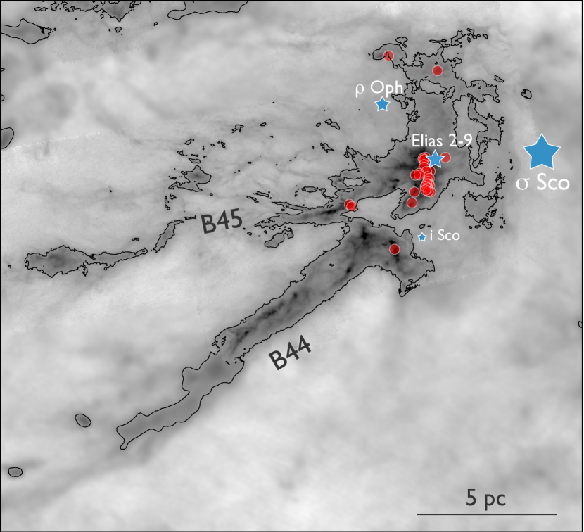
Figure 12: The B44 and B45 filaments and the L1688 cloud containing a cluster of embedded protostars (red circles). The linear distribution of protostars in the L1688 cluster is orthogonal to the projected line-of-sight to $\sigma$-Sco, suggesting star formation in a compression front. The head of B45 (L1709) is radially aligned with $\sigma$ Sco, while B44 is radially aligned with Elias 2-9 (HD147889).

Table 3: Overview of the Herschel data used in the paper

Archival name	Obs. ID	R.A.	Dec.	Wavelengths ($\mu$m)	Obs. Date
Sco-06	1342263838/9	245.39	-19.86	250, 350, 500	2013-02-17
Sco-05	1342263840/1	246.62	-19.63	250, 350, 500	2013-02-17
roph_L1688	1342205093/4	246.70	-24.18	250, 350, 500	2010-09-25
Sco-04	1342263842/3	247.89	-19.37	250, 350, 500	2013-02-18
Sco-L43	1342263844/5	248.45	-15.80	250, 350, 500	2013-02-18
roph_north_stream	1342214577/8	249.79	-22.00	250, 350, 500	2011-02-20
roph_L1712	1342204088/9	250.03	-24.12	250, 350, 500	2010-09-05
Sco-01	1342267724/5	252.03	-10.34	250, 350, 500	2013-03-16
Sco-02	1342267726/7	252.04	-12.29	250, 350, 500	2013-03-16
Sco-03	1342267754/5	252.39	-14.78	250, 350, 500	2013-03-17
Sco-CB68	1342267756/7	253.87	-15.84	250, 350, 500	2013-03-17

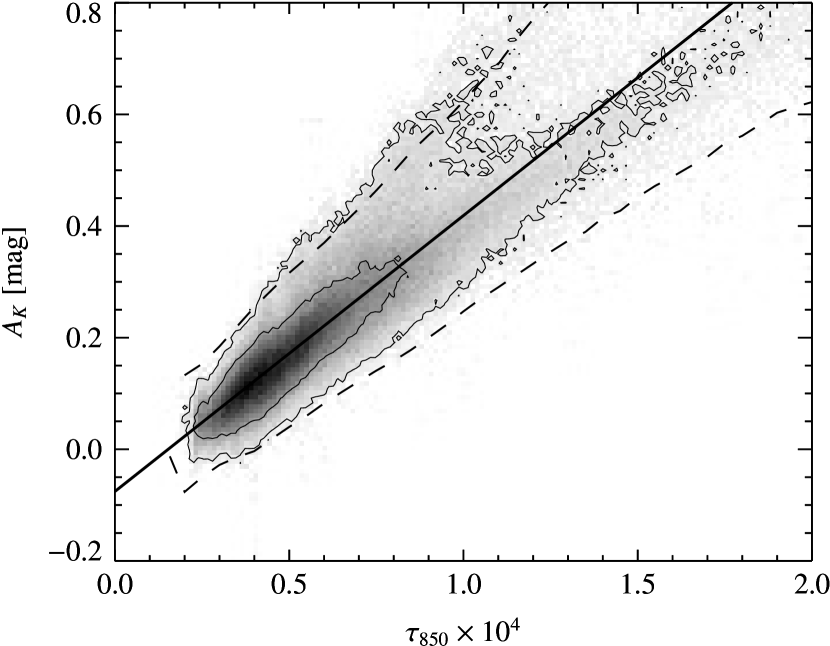
Figure 13: Relationship between submillimeter optical-depth and NIR extinction in Ophiuchus. The best linear fit, used to calibrate the data, is shown together with the expected $3\sigma$ region, as calculated from direct error propagation in the extinction map.

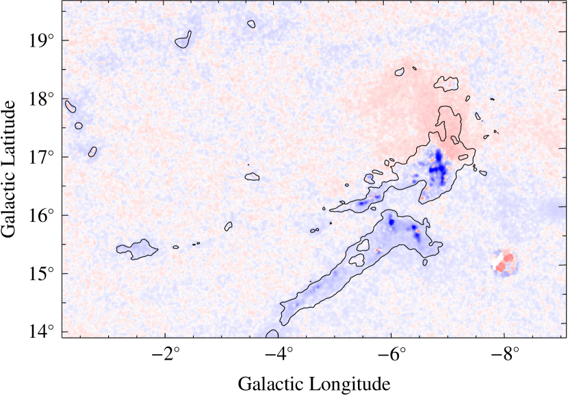
Figure 14: Difference between the extinction predicted by Herschel and the extinction measured with 2MASS/Nicest, with blue (red) indicating a positive (negative) difference.

Appendix B Error maps

In this section, we show the error maps for the Herschel/Planck column density and temperature maps presented in Figure 2 and Figure 3.

Appendix C SIMBAD Objects

Barn68 Ophiuchus Molecular Cloud Lupus Cloud Pipe Nebula sigma Sco pi Sco delta Sco zeta Oph beta Sco pi Sco nu Sco rho Sco tau Sco 9 Sco rho Oph chi Oph 13 Sco 2 Sco b Sco i Sco lambda Lib V1040 Sco HR5934 Antares HD147889 barn 40 barn 44 barn 45 upper sco L1712