A graph-based approach to entanglement entropy of quantum error correcting codes

Abstract

We develop a graph-based method to study the entanglement entropy of Calderbank-Shor-Steane quantum codes. This method offers a straightforward interpretation for the entanglement entropy of quantum error correcting codes through graph-theoretical concepts, shedding light on the origins of both the local and long-range entanglement. Furthermore, it inspires an efficient computational scheme for evaluating the entanglement entropy. We illustrate the method by calculating the von Neumann entropy of subsystems in toric codes and a special type of quantum low-density-parity check codes, known as bivariate bicycle codes, and by comparing the scaling behavior of entanglement entropy with respect to subsystem size. Our method provides a new perspective for understanding the entanglement structure in quantum many-body systems.

Introduction. Entanglement plays a crucial role in understanding the physics of quantum many-body systems, including topological matters Kitaev and Preskill (2006); Levin and Wen (2006); Eisert et al. (2010), the black hole information paradox Hawking (1976); Page (1993), information scrambling in a thermalization process Hayden and Preskill (2007), the connection between geometry and entanglement in quantum gravity Almheiri et al. (2015); Pastawski et al. (2015), and symmetry breaking/restoration Ares et al. (2023, 2024); Liu et al. (2024). In particular, the scaling law of the entanglement entropy with respect to subsystem size reveals key properties of quantum systems, e.g., discriminating critical and non-critical phases Vidal et al. (2003); Latorre et al. (2003).

Entanglement is introduced in quantum error correcting codes to encode logical information in a non-local manner and protect it from local errors Shor (1995). This is manifested in their notable feature of local indistinguishability Knill and Laflamme (1997); Bennett et al. (1996). There exists a trade-off between the amount of entanglement and the code distance Bravyi et al. (2024a); Li et al. (2024): the lower bound of the geometric entanglement is proportional to the code distance, which implies that more entanglement is required to correct more errors.

Given the unique role of entanglement in quantum error correcting codes, it is important to develop methods to calculate the amount of entanglement within quantum codes. A group-theoretical method to evaluate the entanglement entropy for stabilizer codes was proposed by Refs. Fattal et al. (2004); Hamma et al. (2005a, b). It was used to study the topological entanglement entropy in toric codes Flammia et al. (2009) and other topological codes Kargarian (2008). Recently, a graph-based method was developed to study higher-rank topological phases Ebisu (2023).

In this paper, we develop a different graph-based method to calculate the explicit form of the reduced density matrix and the entanglement entropy of Calderbank-Shor-Steane (CSS) quantum codes. It provides a clear picture on the origin of the local entanglement, which indicates the area law, and the long-range topological entanglement in the toric codes. Furthermore, it inspires an efficient algorithm to evaluate the entanglement entropy for all CSS codes, e.g., quantum low-density-parity-check (qLDPC) codes Tillich and Zémor (2013); Kovalev and Pryadko (2013); Breuckmann and Terhal (2016); Panteleev and Kalachev (2021); Breuckmann and Eberhardt (2021a); Panteleev and Kalachev (2022); Leverrier and Zémor (2022); Higgott and Breuckmann (2023); Wang et al. (2023); Lin and Pryadko (2024); Breuckmann and Eberhardt (2021b). We demonstrate the graph-based method by calculating the entanglement entropy of the bivariate-bicycle codes Bravyi et al. (2024b) and studying its scaling law with respect to the size of the subsystem.

Two-dimensional toric code. We briefly introduce some basic concepts in graph theory Diestel (2024) that are essential for the subsequent discussions. A graph $G(V,E)$ consists of a set of vertices $V$ and a set of edges $E$. An edge connecting two vertices $v_{i},v_{j}\in V$ is represented by the pair $(v_{i},v_{j})$.

A path is a sequence of distinct vertices connected by edges, and a cycle is a path that starts and ends at the same vertex. A connected graph is one in which there exists at least one path between any pair of vertices. A tree graph is a connected graph that contains no cycles. A spanning tree of a graph $G$ is a tree subgraph that includes all the vertices of $G$.

Two-dimensional toric codes can be represented by simple two-dimensional graphs, where qubits are placed on edges. The vertices and faces of the graph represent stabilizers of type $X$ and $Z$, respectively Kitaev (2003). There are two distinct sets of cycles in the graph, the contractible cycles and non-contractible cycles. The former corresponds to $Z$-type stabilizers, while the latter represents logical Pauli $Z$ operators. Since all stabilizers have an eigenvalue of one in the code subspace, the sum of qubit values along any contractible cycle is zero (mod 2), imposing a constraint on these qubit values. The sum of qubit values along a non-contractible cycle can be either 0 or 1, depending on the specific logical state. If one of the logical Pauli $Z$ operators takes a specific eigenvalue, the qubit values along the corresponding non-contractible cycle are also subject to a constraint.

We are concerned with the reduced density matrix and the von Neumann entropy of a subsystem $A$, a subset of qubits, of a toric code. The remaining qubits of the toric code are in the complementary subsystem $B$, as shown in Fig. 1. There are cycles that are entirely enclosed by subsystem $A$ or subsystem $B$, as well as cycles shared by both subsystems, which are referred to as boundary stabilizers. The boundary of subsystem $A$, denoted as $\partial A$, is defined as the set of edges (qubits) that belong to the boundary stabilizers but are not part of subsystem $A$.

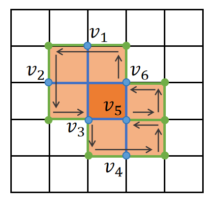
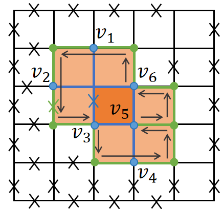
Figure 1: Illustration of subsystems and their spanning trees in a toric code that is embedded in a square lattice with periodic boundary conditions. (a) Subsystem $A$ consists of qubits attached on blue edges and contains one cycle as indicated by the orange face. Subsystem $B$ consists of qubits that are not included in subsystem $A$. The stabilizer operators shared by both subsystems $A$ and $B$ are indicated by pink faces. The boundary of subsystem $A$ is represented by green edges. The gray arrows indicate the closed shortest walk along the boundary. (b) The spanning tree of subsystem $A$ is obtained by removing one of the four qubits (blue cross) along the orange cycle. The spanning tree of subsystem $B$ is obtained by removing appropriate qubits (black crosses) in subsystem $B$ and one qubit along the boundary (green cross). The blue vertices labelled by $\{v_{i}\}$ are the common vertices between the spanning trees of $A$ and $B$.

Consider a connected subsystem $A$ that contains only contractible cycles and its boundary divides a plane into two regions, which are connected areas surrounded by the edges of $\partial A$. The boundary of a region includes the vertices and edges that are incident to the region, and contains a single cycle, as shown in Fig. 1. The qubit values along a cycle are not independent because they are subject to a constraint. In particular, the value of one qubit is fully determined by the values of the remaining independent quibts along the cycle. This implies that taking into account the values of the independent qubits and the constraint is sufficient to determine the state of all qubits along the cycle. From the perspective of graph theory, this is equivalent to deleting one edge from the cycle and transforming it into a path. For a system that contains many cycles, one can selectively delete appropriate edges to remove all cycles, resulting in a spanning tree. The state of the system is then fully determined by the independent qubits in the spanning tree and the associated constraints.

To facilitate further discussion in the language of graph theory, we map subsystems $A$ and $B$, as well as the boundary $\partial A$, to graphs by incorporating their vertices. The symbols $A$, $B$ and $\partial A$ are used to refer to both the sets of qubits and their corresponding graphs. By deleting the appropriate edges to remove all the cycles within the graphs $A$ and $B$, we obtain spanning trees $T_{A}(V_{T_{A}},E_{T_{A}})$ and $T_{B}(V_{T_{B}},E_{T_{B}})$, respectively. Since the boundary $\partial A$ is a subgraph of $B$ and contains a single cycle, we delete one edge from the cycle. The union of the spanning trees $T_{A}$ and $T_{B}$ forms joint cycles, introducing new constraints. This implies that the state of subsystem $A$ depends on the state of subsystem $B$, and vice versa.

The overlap between the set of vertices of the spanning tree $T_{A}$ and that of the boundary $\partial A$ is denoted as $V_{T_{A}}\bigcap V_{\partial A}=\left\{v_{1},....,v_{m}\right\}$, where $m$ represents the total number of common vertices. These vertices are ordered counterclockwise along the shortest closed walk on the boundary, with $v_{1}$ chosen arbitrarily, as shown in Fig. 1. We now partition the boundary into $m$ paths based on the common vertices,

$$\partial A=P^{v_{1},v_{2}}_{\partial A}\bigcup P^{v_{2},v_{3}}_{\partial A}\bigcup\cdots\bigcup P^{v_{m-1},v_{m}}_{\partial A}\bigcup P^{v_{m},v_{1}}_{\partial A},$$ (1)

where $P^{v_{i},v_{i+1}}_{{\partial A}}$ is a path on the boundary that includes edges between the vertex $v_{i}$ and the vertex $v_{i+1}$. Because $T_{A}$ is the spanning tree, there is a unique path between the vertex $v_{i}$ and the vertex $v_{i+1}$, which is denoted as $P^{v_{i},v_{i+1}}_{A}$. The union of $P^{v_{i},v_{i+1}}_{A}$ for all values of $i$ forms the spanning tree $T_{A}$,

$$T_{A}=P^{v_{1},v_{2}}_{A}\bigcup P^{v_{2},v_{3}}_{A}\bigcup\cdots\bigcup P^{v_{m-1},v_{m}}_{A}\bigcup P^{v_{m},v_{1}}_{A}.$$ (2)

Since one of the edges on the boundary $\partial A$ has been deleted, there are $m-1$ pairs of $(P^{v_{i},v_{i+1}}_{{\partial A}},P^{v_{i},v_{i+1}}_{A})$ that form joint cycles. Define the sum of the qubit values in the path $P^{v_{i},v_{i+1}}_{{\partial A}}$ as $\Sigma^{v_{i},v_{i+1}}_{\partial A}$, and that in the path $P^{v_{i},v_{i+1}}_{A}$ as $\Sigma^{v_{i},v_{i+1}}_{A}$. These joint cycles give rise to $m-1$ constraints, which can be expressed as

$$\Sigma^{v_{i},v_{i+1}}_{\partial A}=\Sigma^{v_{i},v_{i+1}}_{A}=C_{\alpha}^{\,i}$$ (3)

for all possible values of $i$, and $C_{\alpha}^{\,i}=0$ or $1$.

For a given set of $\{C_{\alpha}^{\,i}\}$ (with $\alpha$ fixed), the $m-1$ constraints given by Eq. (3) impose $m-1$ constraints on the qubit values in the spanning tree of subsystem $A$. Since there are $|E_{T_{A}}|$ qubits in the spanning tree of subsystem $A$, the remaining $|E_{T_{A}}|-m+1$ qubits are independent. The qubit configurations of subsystem $A$ span a subspace $\Lambda_{\alpha}^{A}$ with dimension $d^{A}_{\alpha}=2^{|E_{T_{A}}|-m+1}$. The state of subsystem $A$ is then an equal superposition of all these allowable qubit configurations,

$$\ket{\psi_{\alpha}}=\frac{1}{\sqrt{d^{A}_{\alpha}}}\sum_{z\in\Lambda_{\alpha}^{A}}\ket{z}=\frac{1}{\sqrt{d^{A}_{\alpha}}}\sum_{z\in\Lambda_{\alpha}^{A}}\ket{z_{1},z_{2},\cdots,z_{n_{A}}}.$$ (4)

Similarly, for a given set of $\{C_{\alpha}^{\,i}\}$ (with $\alpha$ fixed), the $m-1$ constraints given by Eq. (3) impose $m-1$ constraints on the qubit values on the boundary $\partial A$. Since there are $|E_{\partial A}|$ qubits on the boundary, the remaining $|E_{\partial A}|-m$ qubits are independent. The qubit configurations of the boundary $\partial A$ span a subspace $\Lambda_{\alpha}^{B}$ with dimension $d^{B}_{\alpha}=2^{|E_{\partial A}|-m}$. The pair of subspaces $(\Lambda^{A}_{\alpha},\Lambda^{B}_{\alpha})$ is uniquely determined by the set $\{C_{\alpha}^{\,i}\}$ with $\alpha$ fixed.

For a different set of $\{C_{\alpha^{\prime}}^{\,i}\}$, it follows from Eq. (3) that the subspaces $\Lambda^{B}_{\alpha}$ and $\Lambda^{B}_{\alpha^{\prime}}$ do not overlap and are therefore orthogonal. Since there are $|E_{\partial A}|-1$ independent qubits in the boundary $\partial A$ before joining the spanning trees $T_{A}$ and $T_{B}$, and the subspaces $\Lambda^{B}_{\alpha}$ and $\Lambda^{B}_{\alpha^{\prime}}$ have the same size, the number of distinct pairs of subspaces $(\Lambda^{A}_{\alpha},\Lambda^{B}_{\alpha})$ is $n_{\Lambda}=2^{m-1}$. After tracing out the degrees of freedom of subsystem $B$, we obtain the density matrix of subsystem $A$,

$$\rho_{A}=\frac{1}{n_{\Lambda}}\sum_{\alpha=1}^{n_{\Lambda}}\ket{\psi_{\alpha}}\bra{\psi_{\alpha}}.$$ (5)

The density matrix $\rho_{A}$ is in a diagonal form, so it is straightforward to calculate the von Neumann entropy, which is given by

$$S_{A}=-\log_{2}(n_{\Lambda})=m-1.$$ (6)

The term $m$ is associated with the cycles formed by joining the spanning tree $T_{A}$ and the boundary $\partial A$, and depends on the size of the boundary $\partial A$, indicating its local nature; while the term $-1$ is associated with the cycle surrounding subsystem $A$ and is independent of the subsystem size, indicating a pattern of long-range entanglement.

The entanglement entropy for the case where the boundary encompasses multiple cycles can also be evaluated (see Appendix B). We explicitly calculate the von Neumann entropy for several types of subsystem within a toric code (see Appendix C for details).

General formalism for CSS codes. A general CSS code Calderbank and Shor (1996); Steane (1996) cannot always be represented by a simple graph like toric and surface codes. However, we can still leverage related concepts in graph theory (such as cycles and spanning trees) and generalize the above graph-based method to calculate the density matrix and von Neumann entropy of a subsystem in a CSS code, using its parity check matrix $H_{Z}$. This is because the multiplication of stabilizer generators can be represented by the addition (mod 2) of row vectors in the parity check matrix $H_{Z}$, and the latter is equivalent to the symmetric difference in the cycle space (see Appendix A for details). The $Z$-type stabilizer generators of CSS codes can be partitioned into three sets: (1) $s_{A}$ generators acting only on qubits within subsystem $A$, denoted as $\big{\{}S_{A}^{(i)}\big{\}}_{i=1}^{s_{A}}$;

(2) $s_{B}$ generators acting only on qubits within subsystem $B$, denoted as $\big{\{}S_{B}^{(i)}\big{\}}_{i=1}^{s_{B}}$;

and (3) $s_{AB}$ generators acting on qubits in both subsystems $A$ and $B$, denoted as $\big{\{}S_{AB}^{(i)}\big{\}}_{i=1}^{s_{AB}}$.

For a specific stabilizer generator $S_{A}^{(i)}$ that acts only on qubits in subsystem $A$, one can delete one of its qubits to remove the cycle. This can be accomplished by first transforming the parity check matrix $H_{Z}$ into a specific form and then deleting the qubit and the stabilizer generator. Suppose we want to delete one of the qubits that the stabilizer $S_{A}^{(i)}$ acts on. The element of the parity check matrix corresponding to the row of $S_{A}^{(i)}$ and the column of this qubit is one. If another stabilizer generator, say $S$, also acts on this qubit, meaning that its element in the corresponding column is also one, we then replace the stabilizer generator $S$ with a new stabilizer generator $S^{\prime}=S_{A}^{(i)}S$, for which the element in the corresponding column becomes zero. We continue this process to replace all other stabilizer generators acting on this qubit with new stabilizer generators. The parity check matrix is then transformed into a form in which this qubit is acted on only by the stabilizer generator $S_{A}^{(i)}$. We delete the qubit and the stabilizer $S_{A}^{(i)}$ from the parity check matrix. The remaining matrix is still a valid parity check matrix, with its rows representing a different set of stabilizer generators. The procedure described above is equivalent to Gaussian elimination. We continue the above procedure to delete all stabilizer generators acting only on qubits in subsystem $A$ and those acting only on qubits in subsystem $B$. The parity matrix is transformed into a form like $M_{AB}=\begin{pmatrix}M_{A}&M_{B}\\ \end{pmatrix}$, which describes the stabilizer generators shared by subsystems $A$ and $B$.

The boundary of subsystem $A$ may contain one or more cycles, which can be generated by multiplying several stabilizer generators shared between $A$ and $B$. This implies that new stabilizer generators can be defined from $M_{AB}$, which act only on qubits on the boundary of subsystem $A$. Similarly, if additional cycles exist within subsystem $A$, new stabilizer generators acting exclusively on qubits in $A$ can be defined from $M_{AB}$. Once all such generators have been identified, the Gaussian elimination procedure, along with appropriate row and column permutations, are applied to $M_{AB}$, transforming it into $W_{AB}$ (see Appendix D for details),

$$W_{AB}=\begin{pmatrix}\mathbb{I}&W_{A}^{\prime}&\boldsymbol{0}&\boldsymbol{0}\\ \boldsymbol{0}&W_{A}&W_{B}&\boldsymbol{0}\\ \boldsymbol{0}&\boldsymbol{0}&W_{B}^{\prime}&\mathbb{I}\end{pmatrix}.$$ (7)

The submatrices $\begin{pmatrix}\mathbb{I}&W_{A}^{\prime}&\boldsymbol{0}&\boldsymbol{0}\end{pmatrix}$ and $\begin{pmatrix}\boldsymbol{0}&\boldsymbol{0}&W_{B}^{\prime}&\mathbb{I}\end{pmatrix}$ represent stabilizer generators enclosed entirely in subsystem $A$ and its boundary $\partial A$, respectively. The submatrix $\begin{pmatrix}W_{A}&W_{B}\\ \end{pmatrix}$ represents stabilizer generators formed by joining the spanning trees of subsystems $A$ and $B$. By reintroducing the deleted qubits and stabilizer generators, the original parity check matrix $H_{Z}$ can be transformed into $\tilde{H}_{Z}$ through Gaussian elimination,

$$\tilde{H}_{Z}=\begin{pmatrix}\mathbb{I}&\tilde{W}_{A}&\boldsymbol{0}&\boldsymbol{0}\\ \boldsymbol{0}&W_{A}&W_{B}&\boldsymbol{0}\\ \boldsymbol{0}&\boldsymbol{0}&\tilde{W}_{B}&\mathbb{I}\end{pmatrix}.$$ (8)

Define the qubit configuration of subsystem $A$ as $|z_{A}\rangle=|z_{A}^{d},z_{A}^{t}\rangle$ and that of subsystem $B$ as $|z_{B}\rangle=|z_{B}^{t},z_{B}^{d}\rangle$,

Here, $|z_{A}^{d}\rangle$ and $\ket{z_{A}^{t}}$ represent the qubit configurations of the deleted and remaining qubits in subsystem $A$, respectively; while $|z_{B}^{d}\rangle$ and $\ket{z_{B}^{t}}$ denote the qubit configurations of the deleted and remaining qubits in subsystem $B$, respectively. The qubit configuration $\ket{z}=\ket{z_{A},z_{B}}$ satisfies $\tilde{H}_{Z}\,z=0$, which implies

$$z_{A}^{d}+\tilde{W}_{A}z_{A}^{t}=0,~~~~z_{B}^{d}+\tilde{W}_{B}z_{B}^{t}=0,$$

$$W_{A}z_{A}^{t}=W_{B}z_{B}^{t}=C_{\alpha},$$ (9)

where $C_{\alpha}$ is a binary vector whose number of components equals to the number of rows of $W_{A}$ and $W_{B}$.

Suppose that the number of remaining qubits in subsystem $A$ is $t_{A}$ and that in subsystem $B$ is $t_{B}$, and the rank of the submatrices $W_{A}$ and $W_{B}$ is $r$. For a given $C_{\alpha}$, there are $2^{t_{A}-r}$ qubit configurations $|z_{A}\rangle$ that satisfy the constraints in Eq. (A graph-based approach to entanglement entropy of quantum error correcting codes). Consequently, these allowable configurations form a subspace $\Lambda_{\alpha}^{A}$ with dimension $d_{\alpha}^{A}=2^{t_{A}-r}$. Similarly, there are $2^{t_{B}-r}$ qubit configurations $\ket{z_{B}}$ for the same $C_{\alpha}$, which form a subspace ${\Lambda}_{\alpha}^{B}$ with dimension ${d}_{\alpha}^{B}=2^{t_{B}-r}$. Different binary vectors $C_{\alpha}$ define mutually orthogonal subspaces for subsystems $A$ and $B$, which implies that the number of pairs of orthogonal subspaces $(\Lambda_{\alpha}^{A},\Lambda_{\alpha}^{B})$ is $n_{\Lambda}=2^{r}$. After tracing out the degrees of freedom of subsystem $B$, the density matrix of subsystem $A$ is given in the same form as Eq. (5), with $n_{\Lambda}=2^{r}$.

One can now straightforwardly calculate the von Neumann entropy,

$$S_{A}=-\log_{2}(n_{\Lambda})=r=\text{rank}(W_{A})=\text{rank}(W_{B}).$$ (10)

Note that the submatrix $\begin{pmatrix}W_{A}&W_{B}\end{pmatrix}$ generates the joint cycle space formed by the spanning trees of $A$ and $B$, therefore the entanglement entropy is equal to the cyclomatic number of the joint cycle space.

For a given parity check matrix $H_{Z}=\begin{pmatrix}H_{A}&H_{B}\\ \end{pmatrix}$, for which $\text{rank}(H_{A})=r_{A}$, $\text{rank}(H_{B})=r_{B}$ and $\text{rank}(H_{Z})=r_{H}$, it can be proved that (see Appendix E for details)

$$S_{A}=r_{A}+r_{B}-r_{H}.$$ (11)

This provides an efficient scheme for evaluating the entanglement entropy, since the rank of a matrix can be calculated efficiently. The entanglement entropy for other logical states can be evaluated similarly by appending rows representing logical Pauli $Z$ operators to the parity check matrix $H_{Z}$ (see Appendix F for details).

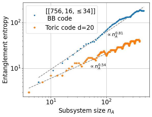
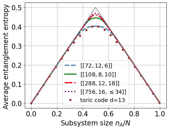
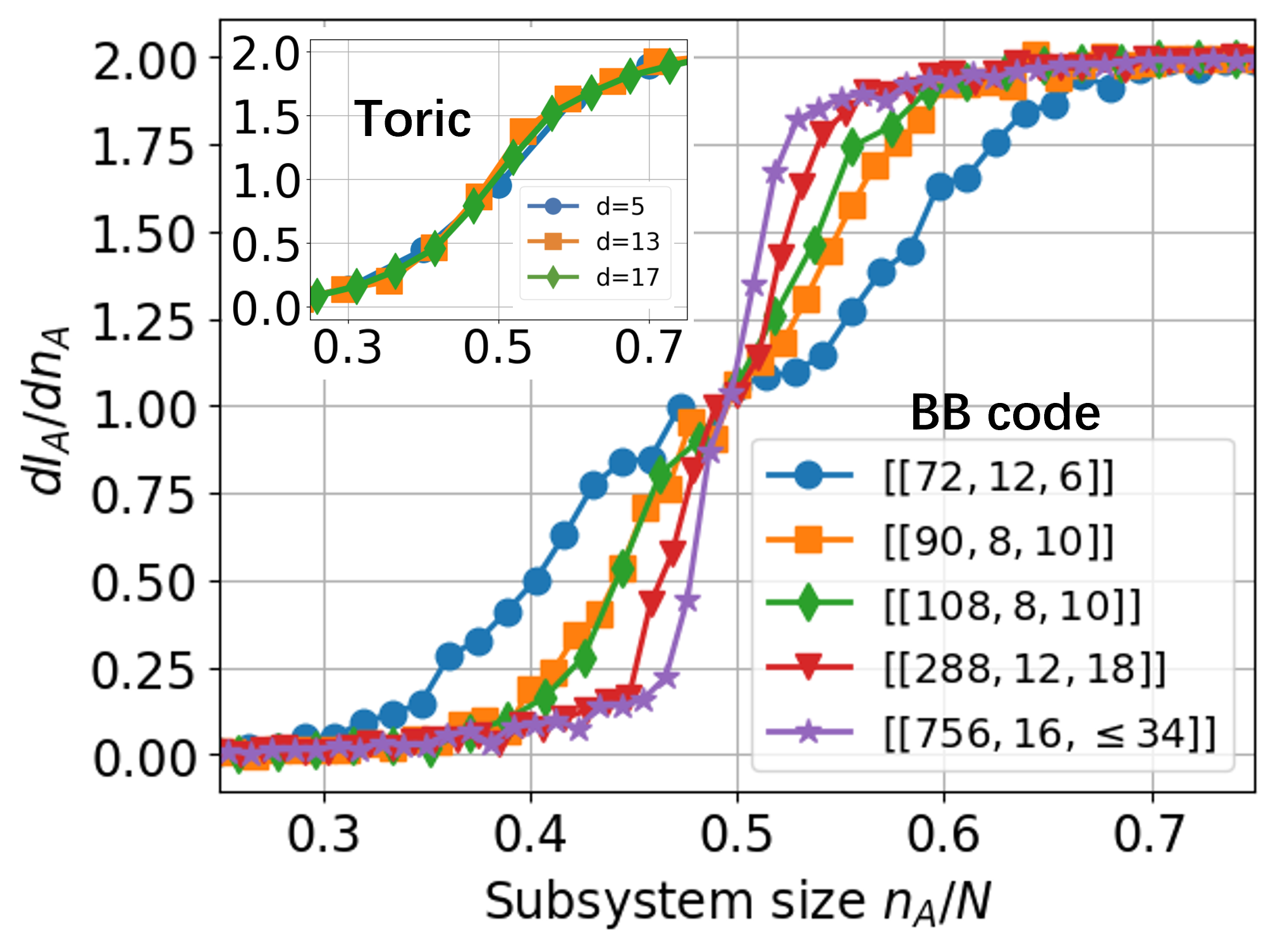
Figure 2: Entanglement entropy of BB codes and toric codes. (a) Scaling behavior of entanglement entropy for subsystems with increasing sizes. The size of the subsystem is chosen to be less than half of the entire system. (b) Averaged entanglement entropy for randomly selecting subsystems. (c) Derivative of the discrepancy of entropy $I_{A}$ for BB codes. The inset shows the same quantity for toric codes.

Entanglement entropy for qLDPC codes. We apply the graph-based method to calculate the entanglement entropy for a family of qLDPC codes called bivariate bicycle (BB) codes Bravyi et al. (2024b). They are quantum codes of CSS type for which each stabilizer generator acts non-trivially on six qubits and each qubit participates in six stabilizer generators. The BB codes are similar to the two-dimensional toric codes except that they are not geometrically local. We show that the entanglement properties of the BB codes differ significantly from those of the two-dimensional toric codes.

A subsystem with a convex disk shape in toric codes encloses nearly the maximum number of stabilizer generators. We select a series of subsystems in BB codes with a similar property (see Appendix G for details).

The von Neumann entropy of the defined subsystems provides insight into their scaling behavior. The entanglement entropy for a toric code with $d=20$ and a BB code $[[756,16,\leq 34]]$ (see Appendix H for code construction) is shown in Fig. 2 (a). The entanglement entropy for the toric code is approximately proportional to $\sqrt{n_{A}}$, consistent with an area law that reflects the localized nature of its entanglement. In contrast, for the BB code, the entanglement entropy scales as $n_{A}^{\gamma}$ with $\gamma\approx 0.81$, showing a faster increase in the entanglement entropy and revealing the presence of more delocalized and long-range entanglement.

Another way to choose a subsystem $A$ is to randomly select a set of qubits from the code. This is in some sense equivalent to fixing a subsystem and averaging over a set of different quantum states. The average entanglement entropy for both toric codes and BB codes is shown in Fig. 2 (b). It is evident that the average entanglement entropy $\bar{S}_{A}$ exhibits a linear increase with respect to the size of the subsystem, $n_{A}$, in the regime where $n_{A}$ is small, suggesting a volume law. It deviates from the volume law when $n_{A}$ approaches half of the total system size and the deviation reaches a maximum at $n_{A}=N/2$. It starts to decrease when $n_{A}>N/2$, and exhibits a linear decrease as $n_{A}$ approaches $N$.

It may seem counterintuitive that the average entanglement entropy of small random subsystems follows a volume law.

This is due to the unique characteristics of the stabilizer codes. When $n_{A}$ is smaller than the number of qubits on which a stabilizer generator acts non-trivially, the state of the subsystem is maximally mixed. As a result, the entanglement entropy contributed by this subsystem is $n_{A}$. When $n_{A}$ exceeds the number of qubits on which a stabilizer generator acts non-trivially, and some of these qubits form one or more stabilizer generators (cycles in the language of graph theory), the entanglement entropy deviates from $n_{A}$. We define the discrepancy between $n_{A}$ and $\bar{S}_{A}$ as a quantitative measure that characterizes the deviation, $I_{A}=n_{A}-\bar{S}_{A}(n_{A})$.

The entropy discrepancy $I_{A}$ depends on the number of independent stabilizer generators that act exclusively within subsystem $A$.

When a randomly selected subsystem is small compared to the entire system, the selected quibts are likely to be disconnected from each other, forming many isolated qubit “islands”. The entanglement entropy of each qubit island is typically equal to its size, with high probability, leading to the observed volume law. The entanglement entropy increases linearly with $n_{A}$ as long as the size of the isolated qubit island remains sufficiently small. Consequently, adding more qubits to subsystem $A$ does not violate the volume law.

As the size of a randomly selected subsystem grows so that a qubit island encompasses one or more stabilizer generators, the average entanglement entropy starts to deviate from the volume law. Beyond this point, adding more qubits to the subsystem increases its entropy discrepancy, and as the subsystem grows further, the rate of change of the entropy discrepancy approaches a constant.

We calculate the rate of change of the entropy discrepancy, ${\rm d}I_{A}/{\rm d}n_{A}$, for both BB codes and toric codes, revealing a significant difference between the two, as shown in Fig. 2 (c). A sharp transition from a phase with a vanishing rate to one with a constant rate is observed for the BB codes, with the transition becoming sharper as the size of the BB codes increases. In contrast, for the toric codes, the transition is much smoother and the steepness of the transition is independent of the size of the toric codes. The difference can be qualitatively understood as follows. The stabilizer generators for the toric codes act non-trivially on four qubits, whereas those for the BB codes act non-trivially on six qubits. As a result, the isolated qubit islands for the BB codes must grow larger than those for the toric codes to break the volume law.

The sharp transition for the rate of change of the entropy discrepancy for the BB codes can be qualitatively understood using concepts from percolation theory Broadbent and Hammersley (1957). A random subsystem of size $n_{A}$ is obtained by randomly selecting $n_{A}$ qubits from a total of $N$ qubits, with each quibt being selected with probability $p_{s}=n_{A}/N$ and discarded with probability $1-p_{s}$. When $p_{s}$ is small, the qubits in subsystem $A$ form many disconnected small qubit islands. However, when $p_{s}$ is sufficiently large, the qubits in subsystem $A$ merge into a few connected, large qubit islands. According to percolation theory, there exists a percolation threshold below which the quibts remain disconnected and above which quibts rapidly become connected. The connectivity of qubits in subsystem $A$ is related to the entropy discrepancy. This implies a close relationship between the phase transition in percolation theory and the observed sharp transition for the rate of change of the entropy discrepancy.

Conclusions. We developed a graph-based method to explore the density matrix and the entanglement entropy of CSS-type quantum error correcting codes. The entanglement entropy has a simple graph-theoretical interpretation: it is the cyclomatic number of the cycle space formed by joining the spanning trees of the subsystem and its complementary subsystem. Its analytic expression related to the matrix rank inspires an efficient scheme to calculate the entanglement entropy for complicated quantum codes, e.g., qLDPC codes. We demonstrated the method by calculating and comparing the entanglement entropy for the toric codes and the BB codes. The graph-based method does not depend on the specific geometry and topology of the quantum systems and can be generalized to explore systems with higher spins and irregular structures, as well as a broader class of stabilizer codes.

Acknowledgements: D. S. is supported by the Fundamental Research Funds for the Central Universities, HUST (Grant No. 5003012068) and Wuhan Young Talent Research Funds (Grant No. 0106012013).

Appendix A Edge space, cycle space and symmetric difference

One can extract a vector space from a graph. The process involves extracting the edge set from a graph, which subsequently allows for the construction of a corresponding vector space based on that set. In graph theory, this space is referred to as the edge space. Before constructing the vector space, it is essential to introduce the concept of symmetric difference between two sets. Given two sets $A$ and $B$, the symmetric difference between $A$ and $B$ is the set of elements that are in either $A$ or $B$, but not in their intersection. This is denoted as $A\Delta B$ and can be expressed mathematically as

$$A\Delta B=(A\setminus B)\cup(B\setminus A),$$ (12)

where the $A\setminus B$ is a set which contains the elements in $A$ but not in $B$.

The edge space comprises the subsets of $E$, where vector addition is defined by the symmetric difference. The basis of the edge space consists of all individual edges, which implies that the dimension of the edge space is equal to the size of the graph. We can map the edge space to a vector space $\Gamma$ over the field $\mathbb{F}_{2}$ whose dimension is the same as the size of the graph. For an edge subset within the edge space, we suppose that it is mapped to the vector $\tau_{1}$ in the space $\Gamma$. If a specific edge is absent, the corresponding component in $\tau_{1}$ is zero; while if the edge is present, the corresponding component is one. As a result, each edge subset can be mapped to a binary vector with dimension of $|E|$. The symmetric difference of two edge subsets corresponds to the addition (mod 2) between two binary vectors in $\Gamma$.

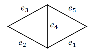
Figure 3: Illustration of the edge space and cycle space in a graph. Consider a given graph, where a basis of the edge space is comprised of the edges $e_{1},e_{2},e_{3},e_{4},e_{5}$. If we consider the edge subsets in $\text{pow}(E)$, $\omega_{1}=\left\{e_{1},e_{4},e_{5}\right\}$ and $\omega_{2}=\left\{e_{2},e_{3},e_{4}\right\}$, the symmetric difference of the two edge subsets is given by $\omega_{1}\Delta\omega_{2}=\left\{e_{1},e_{2},e_{3},e_{5}\right\}$. This operation demonstrates the combination of edges resulting from the symmetric difference, which is a key concept in understanding the edge space and its algebraic structure. The corresponding vectors for $\omega_{1}$ and $\omega_{2}$ in $\Gamma$ are $(1,0,0,1,1)$ and $(0,1,1,1,0)$, respectively. $\omega_{1}\Delta\omega_{2}$ corresponds to the addition (mod 2) of $(1,0,0,1,1)$ and $(0,1,1,1,0)$. $(1,0,0,1,1)+(0,1,1,1,0)=(1,1,1,0,1)$ means that $\omega_{1}\Delta\omega_{2}=\left\{e_{1},e_{2},e_{3},e_{5}\right\}$. The cycle space contains three cycles $\left\{e_{1},e_{4},e_{5}\right\},\left\{e_{2},e_{3},e_{4}\right\},\left\{e_{1},e_{2},e_{3},e_{5}\right\}$. The dimension of the cycle space is 2.

The cycle space of a graph $G$ consists of all cycles in the graph, denoted as $c(G)$. It is a subspace of the edge space. The vector addition of cycle space also amounts to the symmetric difference. The basis of the cycle space is the minimal set of cycles which can span all the cycles in the graph. The dimension of the cycle space is defined as the number of elements in the basis, which is called cyclomatic number.

Consider a parity check matrix $H_{Z}$, the multiplication of two stabilizer generators is equivalent to the addition (mod 2) of two binary vectors of its row space. All the stabilizers are generated by multiplying several stabilizer generators in the parity check matrix. Therefore, we can regard all independent generators as a basis of a cycle space. Each stabilizer corresponds to a cycle in the cycle space and the qubits associated with the stabilizers can be regarded as the edges of the cycle.

Appendix B Multiple boundary cycles

It is possible that the boundary $\partial A$ divides a plane into $\ell+1$ regions, with $\ell$ internal regions that are bounded by the edges of $\partial A$ and are denoted as $\{R_{\mu}\}_{\mu=1}^{\ell}$. In this case, there are only $|E_{\partial A}|-\ell$ independent qubits and $2^{|E_{\partial A}|-\ell}$ distinct qubit configurations in the boundary $\partial A$. Denote the boundary of these regions as $\{\partial R_{\mu}\}_{\mu=1}^{\ell}$. Suppose the overlap between the set of vertices of the spanning tree $T_{A}$ and that of the region boundary $\partial R_{\mu}$ is $V_{T_{A}}\bigcap V_{\partial R_{\mu}}=\left\{v_{1}^{(\mu)},\cdots,v_{m_{\mu}}^{(\mu)}\right\}$, where $m_{\mu}$ is the total number of common vertices and the index $\mu$ indicates which region boundary these common vertices belong to. The common vertices are ordered counterclockwise along the shortest closed walk along the region boundary $\partial R_{\mu}$ and $v_{1}^{(\mu)}$ can be chosen arbitrarily. Divide the region boundary $\partial R_{\mu}$ as subsets based on the common vertices as follows,

$$\partial R_{\mu}=\partial R_{\mu}^{v_{1},v_{2}}\bigcup\partial R_{\mu}^{v_{2},v_{3}}\bigcup\cdots\bigcup\partial R_{\mu}^{v_{m_{\mu}},v_{1}},$$ (13)

where $\partial R_{\mu}^{v_{j},v_{j+1}}$ is the path on the region boundary $\partial R_{\mu}$ between the vertex $v_{j}^{(\mu)}$ and the vertex $v_{j+1}^{(\mu)}$. This path does not contain other common vertices. Note that we have ignored the index $\mu$ associated with $v_{j}^{(\mu)}$ in Eq. (13) because information about the region boundary has already been indicated by the lower index of $\partial R_{\mu}$.

There is only one path between the vertex $v_{j}^{(\mu)}$ and the vertex $v_{j+1}^{(\mu)}$ in the spanning tree $T_{A}$, denoted as $P_{A[\mu]}^{v_{j},v_{j+1}}$. Since one of the edges in $\partial R_{\mu}$ has been deleted, there are $(m_{\mu}-1)$ pairs of $(\partial R_{\mu}^{v_{j},v_{j+1}},P_{A[\mu]}^{v_{j},v_{j+1}})$ that form joint cycles. Define the sum of qubit values in the edge set $E_{\partial R_{\mu}}^{v_{j},v_{j+1}}$ of the path $\partial R_{\mu}^{v_{j},v_{j+1}}$ as $S_{\partial R_{\mu}}^{v_{j},v_{j+1}}$, and that in the edge set $E_{P_{A[\mu]}}^{v_{j},v_{j+1}}$ of the path $P_{A[\mu]}^{v_{j},v_{j+1}}$ as $S_{A[\mu]}^{v_{j},v_{j+1}}$, namely,

$$S_{\partial R_{\mu}}^{v_{j},v_{j+1}} = \sum_{(v,\bar{v})\in E_{\partial R_{\mu}}^{v_{j},v_{j+1}}}z_{(v,\bar{v})},$$

$$S_{A[\mu]}^{v_{j},v_{j+1}} = \sum_{(v^{\prime},\bar{v}^{\prime})\in E_{P_{A[\mu]}}^{v_{j},v_{j+1}}}z_{(v^{\prime},\bar{v}^{\prime})},$$ (14)

where $z_{(v,\bar{v})}$ and $z_{(v^{\prime},\bar{v}^{\prime})}$ represent qubit values in the edge sets $E_{\partial R_{\mu}}^{v_{j},v_{j+1}}$ and $E_{P_{A[\mu]}}^{v_{j},v_{j+1}}$, respectively. These boundary cycles give rise to $m_{\mu}-1$ constraints, which can be expressed as

$$S_{\partial R_{\mu}}^{v_{j},v_{j+1}}+S_{A[\mu]}^{v_{j},v_{j+1}}=0$$ (15)

or

$$S_{\partial R_{\mu}}^{v_{j},v_{j+1}}=S_{A[\mu]}^{v_{j},v_{j+1}}=C_{\alpha}^{\mu,j}$$ (16)

for all possible value of $j$, and $C_{\alpha}^{\mu,j}\in\{0,1\}$. Taking into account $\ell$ boundary regions, there are $\sum_{\mu=1}^{\ell}m_{\mu}-\ell$ constraints in total.

When the qubit values on the boundary $\partial A$ are fixed, constraints given by Eq. (16) are reduced to $\sum_{\mu=1}^{\ell}m_{\mu}-\ell$ constraints to the qubit values in the spanning tree $T_{A}$. The allowable qubit configurations of subsystem $A$ span a subspace $\Lambda_{\alpha}^{A}$ of dimension $d^{A}_{\alpha}=2^{|E_{T_{A}}|-\sum_{\mu}m_{\mu}+\ell}$. The state of subsystem $A$ is an equal superposition of all these qubit configurations,

$$|\psi_{\alpha}\rangle=\frac{1}{\sqrt{d^{A}_{\alpha}}}\sum_{z\in\Lambda_{\alpha}^{A}}|z\rangle=\frac{1}{\sqrt{d^{A}_{\alpha}}}\sum_{z\in\Lambda_{\alpha}^{A}}|z_{1},z_{2},\cdots,z_{n_{A}}\rangle.$$ (17)

For all qubit configurations in $\Lambda_{\alpha}^{A}$, $S_{A[\mu]}^{v_{j},v_{j+1}}$ are fixed for all values of $\mu$ and $j$. In this case, the qubit configurations of the boundary $\partial A$ that satisfy Eq. (16) span a subspace $\Lambda_{\alpha}^{B}$ with dimension $d^{B}_{\alpha}=2^{|E_{\partial A}|-\sum_{\mu}m_{\mu}}$. The mapping between the subspaces $\Lambda_{\alpha}^{A}$ and $\Lambda_{\alpha}^{B}$ is one-to-one, since they are determined by a fixed set of values $S_{A[\mu]}^{v_{j},v_{j+1}}$.

For a different set of values $C_{\alpha^{\prime}}^{\mu,j}$, it is evident from Eq. (16) that the subspaces $\Lambda_{\alpha}^{B}$ and $\Lambda_{\alpha^{\prime}}^{B}$ have no overlap and are therefore orthogonal. Since there are $|E_{\partial A}|-\ell$ independent qubits before joining the spanning trees $T_{A}$ and $T_{B}$, and the subspaces $\Lambda_{\alpha}^{B}$ and $\Lambda_{\alpha^{\prime}}^{B}$ have the same size, the number of different pairs of subspaces $(\Lambda_{\alpha}^{A},\Lambda_{\alpha}^{B})$ is

$$n_{\Lambda}=\frac{2^{|E_{\partial A}|-\ell}}{d_{\alpha}^{B}}=\frac{2^{|E_{\partial A}|-\ell}}{2^{|E_{\partial A}|-\sum_{\mu}m_{\mu}}}=2^{\sum_{\mu}m_{\mu}-\ell}.$$ (18)

After tracing out the degrees of freedom of subsystem $B$, we obtain the density matrix of subsystem $A$,

$$\rho_{A}=\frac{1}{n_{\Lambda}}\sum_{\alpha=1}^{n_{\Lambda}}|\psi_{\alpha}\rangle\langle\psi_{\alpha}|.$$ (19)

The density matrix $\rho_{A}$ is in a diagonal form, so it is straightforward to calculate the von Neumann entropy, which is equal to

$$S_{A}=-\log_{2}(n_{\Lambda})=\sum_{\mu=1}^{\ell}m_{\mu}-\ell.$$ (20)

The edges in every pair of subgraphs $(\partial R_{\mu}^{v_{j},v_{j+1}},P_{A[\mu]}^{v_{j},v_{j+1}})$ constitute one joint cycle. One needs to delete one edge in each region boundary cycle. If the deleted edge lies at the intersection of two joint cycles, the two faces formed by the two joint cycles become connected. In another case, if the deleted edge is incident with both the face formed by a joint cycle and the external region, the two regions become connected. In both cases, deleting an edge reduces one face formed by the joint cycles. Before the process of deleting an edge in each region boundary, there are a total of $\sum_{\mu}m_{\mu}$ faces formed by the joint cycles. After deleting $\ell$ edges, the number of remaining faces is $\sum_{\mu}m_{\mu}-\ell$, which corresponds to the entanglement entropy.

Appendix C Some examples in toric codes

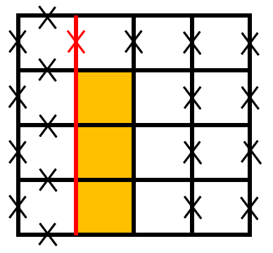
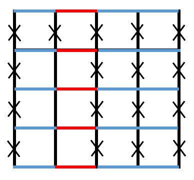
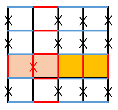
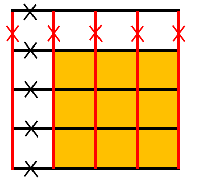
Figure 4: Illustration of subsystems in the toric code, and their spanning trees and joint cycles. These subsystems are the qubits on the red edges. (a) The spanning tree of subsystem $A$ is obtained by removing one of the $d$ qubits (red cross) along the non-contractible qubit chain. The spanning tree of subsystem $B$ is obtained by removing appropriate qubits (black cross) in subsystem $B$. The joint cycles are indicated by the orange faces. (b) The spanning forest of subsystem $A$ consists of the qubits on the red edges. The spanning tree of subsystem $B$ is obtained by removing appropriate qubits (black cross) in subsystem $B$. The qubits of $B$ on the blue edges form non-contractible joint cycles with the edges in the spanning forest of $A$. (c) The red edges, with the exception of the one that has been removed (red cross), constitute the spanning forest of subsystem $A$. By removing the edges indicated by the black cross, one can obtain the spanning tree of subsystem $B$. The spanning forest of $A$ and the spanning tree of $B$ share the stabilizer operators that are indicated by one pink face and $d-2$ orange faces. The red edges and the blue edges also form non-contractible joint cycles. (d) The spanning forest of subsystem $A$ and that of subsystem $B$ form a joint cycle space. Two spanning forests share the stabilizer operators which are indicated by the orange faces.

We calculate the entanglement entropy for several types of subsystem for the logical state $|00\rangle_{L}$, including a single qubit, two qubits, the qubit chain, the vertical qubit ladder, the cross and all vertical qubits. Some of these subsystems are shown in Fig. 4.

C.1 One qubit

Suppose that subsystem $A$ contains a single qubit, which participates in two $Z$-type stabilizer generators. The boundary of subsystem $A$ contains only one cycle. After deleting a qubit from the boundary to remove the cycle, the qubit in subsystem $A$ and the spanning tree of subsystem $B$ form one joint cycle. Therefore, the entanglement entropy is 1.

C.2 Two qubits

Suppose that subsystem $A$ contains two qubits. These two qubits belong to either a single $Z$-type stabilizer generator, or two distinct $Z$-type stabilizer generators. In the former case, subsystem $A$ and its boundary form 3 stabilizer generators, and the boundary contains one cycle. Therefore, the entanglement entropy is 2. In the latter case, subsystem $A$ and its boundary form 4 stabilizer generators, and the boundary contains two cycles. Consequently, the entanglement entropy is 2.

C.3 The qubit chain

Consider a $d\times d$ square lattice and a non-contractible qubit chain in the torus, as shown by the red edges in Fig. 4 (a). The spanning tree of subsystem $A$ and that of subsystem $B$ form a joint cycle space with dimension $d-1$. Therefore, the entanglement entropy for the non-contractible qubit chain is $d-1$.

C.4 The vertical qubit ladder

Suppose that the qubits in subsystem $A$ form a vertical ladder, as shown by the red edges in Fig. 4 (b). The qubits in the vertical ladder are disconnected, forming multiple spanning trees, which is known as the spanning forest. The spanning forest of subsystem $A$ and the spanning tree of subsystem $B$ form $d$ parallel non-contractible joint cycles. Therefore, the entanglement entropy is $d$.

C.5 The cross

The qubits in subsystem $A$ form a cross, as shown by the red edges in Fig. 4 (c). The spanning forest of subsystem $A$ and the spanning tree of subsystem $B$ form a joint cycle space. A basis of the joint cycle space consists of $d-1$ contractible cycles, represented by a pink face and orange faces, along with $d$ non-contractible cycles.The cyclomatic number of the cycle space is given by $2d-1$, which directly corresponds to the entanglement entropy of the system. Hence, the entanglement entropy is $2d-1$.

C.6 All vertical qubits

The subsystem $A$ contains all vertical qubits in the torus, as shown by the red edges in Fig. 4 (d). By removing all the vertical edges in the first row, one can obtain the spanning forest of $A$. Similarly, the spanning forest of $B$ can be obtained by removing all horizontal edges from the first column. The spanning forest of $A$ and that of $B$ form a cycle space with dimension $(d-1)^{2}$, as shown in Fig. 4 (d). The entanglement entropy is $(d-1)^{2}$.

Appendix D Transformation of parity check matrix

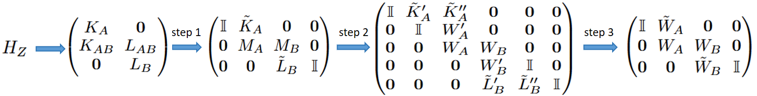
Figure 5: The process for transforming the parity check matrix. Prior to step 1, appropriate row and column permutations are applied to reorganize the parity check matrix. Step 1 involves deleting the cycles within subsystem $A$ that do not intersect with the boundary of subsystem $B$, as well as the cycles within subsystem $B$ that do not intersect with the boundary of subsystem $A$. Step 2 focuses on eliminating the cycles that lie on the boundaries of both subsystems $A$ and $B$. Step 3 entails transforming the parity check matrix into its final form through Gaussian elimination.

We provide a detailed process of transforming the parity check matrix $H_{Z}$, as summarized in Fig. 5. Once subsystems $A$ and $B$ are defined, the parity check matrix $H_{Z}$ of a CSS code can be partitioned into $(H_{A}~H_{B})$ through appropriate column permutations, where $H_{A}$ and $H_{B}$ are submatrices whose columns correspond to qubits in subsystems $A$ and $B$, respectively. By further appropriate row permutations, the parity check matrix can be transformed into

$$\begin{pmatrix}K_{A}&\boldsymbol{0}\\ K_{AB}&L_{AB}\\ \boldsymbol{0}&L_{B}\end{pmatrix},$$ (21)

where the submatrix $(K_{A}~\boldsymbol{0})$ represents stabilizer generators acting non-trivially on qubits only in subsystem $A$, $(\boldsymbol{0}~L_{B})$ represents stabilizer generators acting non-trivially on qubits only in subsystem $B$, and $(K_{AB}~L_{AB})$ represents stabilizer generators acting non-trivially on qubits both in subsystems $A$ and $B$.

For a specific stabilizer generator acting solely on qubits within subsystem $A$, one selects an arbitrary qubit associated with the stabilizer for deletion. Before deleting the qubit, one can employ Gaussian elimination to eliminate all non-zero elements in the column corresponding to this qubit, with the exception of the entry in the row representing the stabilizer generator. By further applying appropriate row and column permutations, the parity check matrix can be transformed into

$$\begin{pmatrix}1&K_{A}^{\prime}&\boldsymbol{0}\\ \boldsymbol{0}&\bar{K}_{A}&\boldsymbol{0}\\ \boldsymbol{0}&K_{AB}^{\prime}&L_{AB}\\ \boldsymbol{0}&\boldsymbol{0}&L_{B}\end{pmatrix},$$ (22)

where the first column indicates which qubit should be removed. For another stabilizer generator acting only on qubits in subsystem $A$, one applies the same procedure. The parity check matrix in Eq. (22) can be transformed into

$$\begin{pmatrix}1&0&K_{A}^{\prime\prime}&\boldsymbol{0}\\ 0&1&\bar{K}_{A}^{\prime}&\boldsymbol{0}\\ \boldsymbol{0}&\boldsymbol{0}&\bar{K}_{A}^{\prime\prime}&\boldsymbol{0}\\ \boldsymbol{0}&\boldsymbol{0}&K_{AB}^{\prime\prime}&L_{AB}\\ \boldsymbol{0}&\boldsymbol{0}&\boldsymbol{0}&L_{B}\end{pmatrix}.$$ (23)

By repeating the above procedure to subsystems $A$ and $B$, the parity check matrix can be transformed into the following form,

$$\begin{pmatrix}\mathbb{I}&\tilde{K}_{A}&\boldsymbol{0}&\boldsymbol{0}\\ \boldsymbol{0}&M_{A}&M_{B}&\boldsymbol{0}\\ \boldsymbol{0}&\boldsymbol{0}&\tilde{L}_{B}&\mathbb{I}\end{pmatrix}.$$ (24)

The columns associated with the two identity matrices correspond to qubits that are needed to be deleted to remove cycles in subsystems $A$ and $B$. The submatrix $M_{AB}\equiv(M_{A}~M_{B})$ represents stabilizer generators shared by subsystems $A$ and $B$.

The boundary of subsystem $A$, namely, the qubits associated with the partition of stabilizer generators $M_{B}$, may contain one or more cycles, which can be generated by multiplying several stabilizer generators shared by $A$ and $B$. This implies that one can always define new stabilizer generators from $M_{AB}$, which act on qubits only in the boundary of subsystem $A$. If such a new generator has been found, we then apply the Gaussian elimination procedure and appropriate row and column permutations to $M_{AB}$, so that it can be transformed into

$$\begin{pmatrix}M_{A}^{\prime}&M_{B}^{\prime}&\boldsymbol{0}\\ \boldsymbol{0}&\tilde{M}_{B}&1\end{pmatrix}.$$ (25)

The new stabilizer generator, represented by $\begin{pmatrix}\boldsymbol{0}&\tilde{M}_{B}&1\end{pmatrix}$, and the qubit intended to be deleted have been moved to the last row and column, respectively. Continue this process to the submatrix $\begin{pmatrix}M_{A}^{\prime}&M_{B}^{\prime}\end{pmatrix}$, one can find all the cycles in the boundary $\partial A$. The parity check matrix can be transformed into

$$\begin{pmatrix}M_{A}^{\prime\prime}&M_{B}^{\prime\prime}&\boldsymbol{0}\\ \boldsymbol{0}&W_{B}^{\prime}&\mathbb{I}\end{pmatrix}.$$ (26)

The submatrix $\begin{pmatrix}\boldsymbol{0}&W_{B}^{\prime}&\mathbb{I}\end{pmatrix}$ represents the stabilizer generators in the boundary of subsystem $A$.

The boundary of subsystem $B$, namely, the qubits associated with the partition of stabilizer generators $M_{A}$, may also contain cycles, which can be generated by multiplying some stabilizer generators represented by the submatrix $\begin{pmatrix}M_{A}^{\prime\prime}&M_{B}^{\prime\prime}\end{pmatrix}$. This implies that one can define new stabilizer generators from $\begin{pmatrix}M_{A}^{\prime\prime}&M_{B}^{\prime\prime}\end{pmatrix}$, which act on qubits only on the boundary of $B$. Following the similar procedure as above, the matrix $M_{AB}$ can be transformed into $W_{AB}$,

$$W_{AB}=\begin{pmatrix}\mathbb{I}&W_{A}^{\prime}&\boldsymbol{0}&\boldsymbol{0}\\ \boldsymbol{0}&W_{A}&W_{B}&\boldsymbol{0}\\ \boldsymbol{0}&\boldsymbol{0}&W_{B}^{\prime}&\mathbb{I}\end{pmatrix}.$$ (27)

The submatrix $\begin{pmatrix}\mathbb{I}&W_{A}^{\prime}&\boldsymbol{0}&\boldsymbol{0}\end{pmatrix}$ represents the stabilizer generators enclosed fully in the boundary of $B$. The columns which have only one nonzero element correspond to the qubits needed to be deleted. All cycles have been removed after deleting appropriate qubits in the boundaries of $A$ and $B$, and the remaining stabilizer generators are represented by the submatrix $\begin{pmatrix}W_{A}&W_{B}\end{pmatrix}$.

At this stage, the original parity check matrix $H_{Z}$ has been transformed into the following form,

$$\begin{pmatrix}\mathbb{I}&\tilde{K}_{A}^{\prime}&\tilde{K}_{A}^{\prime\prime}&\boldsymbol{0}&\boldsymbol{0}&\boldsymbol{0}\\ \boldsymbol{0}&\mathbb{I}&W_{A}^{\prime}&\boldsymbol{0}&\boldsymbol{0}&\boldsymbol{0}\\ \boldsymbol{0}&\boldsymbol{0}&W_{A}&W_{B}&\boldsymbol{0}&\boldsymbol{0}\\ \boldsymbol{0}&\boldsymbol{0}&\boldsymbol{0}&W_{B}^{\prime}&\mathbb{I}&\boldsymbol{0}\\ \boldsymbol{0}&\boldsymbol{0}&\boldsymbol{0}&\tilde{L}_{B}^{\prime}&\tilde{L}_{B}^{\prime\prime}&\mathbb{I}\end{pmatrix}.$$ (28)

where we have partitioned the submatrix $\tilde{K}_{A}$ into $(\tilde{K}_{A}^{\prime}~\tilde{K}_{A}^{\prime\prime})$, and the submatrix $\tilde{L}_{B}$ into $(\tilde{L}_{B}^{\prime}~\tilde{L}_{B}^{\prime\prime})$. By using the rows in the submatrix $\begin{pmatrix}\boldsymbol{0}&\mathbb{I}&W_{A}^{\prime}&\boldsymbol{0}&\boldsymbol{0}&\boldsymbol{0}\end{pmatrix}$ to eliminate the non-zero elements in the block $\tilde{K}_{A}^{\prime}$, and the rows in the submatrix $\begin{pmatrix}\boldsymbol{0}&\boldsymbol{0}&\boldsymbol{0}&W_{B}^{\prime}&\mathbb{I}&\boldsymbol{0}\end{pmatrix}$ to eliminate the non-zero elements in the block $\tilde{L}_{B}^{\prime\prime}$, the parity check matrix can be transformed into

$$\tilde{H}_{Z}=\begin{pmatrix}\mathbb{I}&\tilde{W}_{A}&\boldsymbol{0}&\boldsymbol{0}\\ \boldsymbol{0}&W_{A}&W_{B}&\boldsymbol{0}\\ \boldsymbol{0}&\boldsymbol{0}&\tilde{W}_{B}&\mathbb{I}\end{pmatrix}.$$ (29)

Appendix E Proof of the formula for entanglement entropy

After appropriate row and column permutations, the parity check matrix $H_{Z}$ can be partitioned into $\begin{pmatrix}H_{A}&H_{B}\end{pmatrix}$. Suppose that $\text{rank}(H_{A})=r_{A}$, $\text{rank}(H_{B})=r_{B}$ and $\text{rank}(H_{Z})=r_{H}$. As a first step, we transform the parity check matrix $H_{Z}$ via Gaussian elimination to the form that contains $r_{H}$ linearly independent rows. We then implement step 1 in Fig. 5 and obtain a matrix as shown in Eq. (24). Suppose that the size of the identity matrix in the first row block in the matrix (24) is $m_{A}$, and that of the identity matrix in the third row block is $m_{B}$, then the rank of $M_{AB}$ is given by

$$r_{AB}=r_{H}-m_{A}-m_{B}.$$ (30)

After detecting all cycles in the boundary of subsystem $A$, the submatrix $M_{AB}$ is transformed into

$$M_{AB}^{\prime\prime}=\begin{pmatrix}M_{A}^{\prime\prime}&M_{B}^{\prime\prime}&\boldsymbol{0}\\ \boldsymbol{0}&W_{B}^{\prime}&\mathbb{I}\end{pmatrix}.$$ (31)

The rank of the submatrix $(M_{A}^{\prime\prime}~M_{B}^{\prime\prime})$ is equal to $\text{rank}(M_{A})$, which is denoted as $r_{A}^{\prime\prime}$.

Since $M_{A}^{\prime\prime}$ is a full rank submatrix, we have

$$r_{A}^{\prime\prime}+m_{A}=r_{A}.$$ (32)

The rank of $M_{B}^{\prime\prime}$ is denoted as $r_{B}^{\prime\prime}$. Since the number of rows in the identity block in Eq. (31) is $r_{AB}-r_{A}^{\prime\prime}$, we have

$$r_{B}^{\prime\prime}+r_{AB}-r_{A}^{\prime\prime}+m_{B}=r_{B}.$$ (33)

After step 2 in Fig. 5, the submatrix $\begin{pmatrix}M_{A}^{\prime\prime}&M_{B}^{\prime\prime}\end{pmatrix}$ is transformed into

$$\begin{pmatrix}\mathbb{I}&W_{A}^{\prime}&\boldsymbol{0}\\ \boldsymbol{0}&W_{A}&W_{B}\end{pmatrix}.$$ (34)

The entanglement entropy is determined by the rank of the submatrix $(W_{A}~W_{B})$, which is equal to the rank of $M_{B}^{\prime\prime}$. According to Eqs. (30), (32) and (33), $r_{B}^{\prime\prime}$ is given by $r_{A}+r_{B}-r_{H}$. Consequently, the entanglement entropy is

$$S_{A}=r_{A}+r_{B}-r_{H}.$$ (35)

Appendix F Entanglement entropy for logical states

When deriving the reduced density matrix and entanglement entropy for general CSS codes, we consider constraints introduced only by stabilizer generators and assume the encoded state to be an equal superposition of all allowable qubit configurations. This is equivalent to considering a state that is an equal superposition of all logical computational bases, namely,

$$\ket{\psi_{L}}=\frac{1}{2^{k/2}}\sum\limits_{C\in\{0,1\}^{k}}\ket{C}_{L},$$ (36)

where $\ket{C}_{L}$ represented a logical computational basis state, and $k$ denotes the number of logical qubits. In fact, our method can also be used to evaluate the entanglement entropy for an equal superposition of a subset of logical computational bases. Denote the logical Pauli $Z$ operators as $\bar{Z}_{1},\bar{Z}_{2},\cdots,\bar{Z}_{k}$, and the corresponding values of logical qubits as $\bar{z}_{1},\bar{z}_{2},\cdots,\bar{z}_{k}$, with $\bar{z}_{i}=\{0,1\}$. If one of the logical qubits takes a specific value, say $\bar{z}_{1}=0$, then the encoded state is subject to an additional constraint. By appending a row representing the logical operator $\bar{Z}_{1}$ to the parity check matrix $H_{Z}$, we can evaluate the entanglement entropy for the state

$$\ket{\psi_{L}^{(1)}}=\frac{1}{2^{(k-1)/2}}\sum_{\bar{z}_{2}}\sum_{\bar{z}_{3}}\cdots\sum_{\bar{z}_{k}}\ket{0,\bar{z}_{2},\cdots,\bar{z}_{k}}_{L}.$$ (37)

Similarly, if a set of logical Pauli $Z$ operators take specific eigenvalues, we can calculate the entanglement entropy by adding rows representing these logical Pauli $Z$ operators to the parity matrix $H_{Z}$ and then apply the graph-based approach.

If the tensor product (in the code subspace) of two logical Pauli $Z$ operators, say $\bar{Z}_{1}\otimes\bar{Z}_{2}$, takes a specific eigenvalue, say $+1$, then the encoded state is subject to an additional constraint. By appending a row representing the logical operator $\bar{Z}_{1}\otimes\bar{Z}_{2}$ to the parity matrix $H_{Z}$, we can evaluate the entanglement entropy for the state

$$\ket{\psi_{L}^{(12)}} = \frac{1}{2^{(k-1)/2}}\bigg{\{}\sum_{\bar{z}_{3}}\sum_{\bar{z}_{4}}\cdots\sum_{\bar{z}_{k}}\ket{0,0,\bar{z}_{3},\cdots,\bar{z}_{k}}_{L}$$ (38)

$$+\sum_{\bar{z}_{3}}\sum_{\bar{z}_{4}}\cdots\sum_{\bar{z}_{k}}\ket{1,1,\bar{z}_{3},\cdots,\bar{z}_{k}}_{L}\bigg{\}}.$$

Similarly, if a set of logical operators, which are in the form of a tensor product of some logical Pauli $Z$ operators, takes specific eigenvalues, we can calculate the entanglement entropy by adding rows representing these logical operators to the parity check matrix $H_{Z}$ and then apply the graph-based approach.

In the special case where every logical Pauli $Z$ operator takes a specific eigenvalue, we actually evaluate the entanglement entropy for a logical computational basis state $\ket{C}_{L}$. It can be proved that the entanglement entropy for any logical basis state is the same as that of the logical basis state $\ket{00\cdots 0}_{L}$, for which the eigenvalues of all logical Pauli $Z$ operators are equal to one Kargarian (2008). This equivalence arises from the fact that any logical basis state $\ket{C}_{L}$ can be transformed into $\ket{00\cdots 0}_{L}$ by applying some logical Pauli $X$ operators to flip the corresponding logical qubits from $0$ to $1$, and any logical Pauli $X$ operator is a tensor product of single-qubit Pauli $X$ operators.

Now the question is how to find the logical Pauli $Z$ operators for general CSS codes. We introduce an algorithm to determine the logical Pauli $Z$ operators for an arbitrary CSS code. The algorithm starts with the set of $m$ Pauli generators, denoted as $\{g_{1},g_{2},\cdots,g_{m}\}$, and proceeds as follows Wilde (2009):

1. If the generator $g_{1}$ commutes with all other generators, set it aside in a “set of processed operators”.

2. If the generator $g_{1}$ anti-commutes with another generator $g_{j}$, modify the remaining generators as follows:

   $$\forall i\in\{2,\cdots,m\},i\neq j$$

   $$g_{i}\to \left\{\begin{array}[]{ccc}g_{i},&[\;g_{i},g_{1}\,]=0,&[\;g_{i},g_{j}\,]=0;\\ g_{i},&\{g_{i},g_{1}\}=0,&\{g_{i},g_{j}\}=0;\\ g_{i}g_{1},&[\;g_{i},g_{1}\,]=0,&\{g_{i},g_{j}\}=0;\\ g_{i}g_{j},&\{g_{i},g_{1}\}=0,&[\;g_{i},g_{j}\,]=0.\end{array}\right.$$

   After the modification, all other generators commute with both $g_{1}$ and $g_{j}$. Then set $g_{1}$ and $g_{j}$ aside in the “set of processed operators”.

3. Execute the above procedure recursively to the remaining generators.

For an arbitrary CSS code, we should first compute the generator matrix $G_{Z}$ from the parity check matrix $H_{Z}$. The procedure can be found in Ref. Nielsen and Chuang (2010). By applying the algorithm to the generator matrix $G_{Z}$, where each row represents an independent generator of the code, the output is a new matrix. By removing the rows of the output that are linearly dependent on the rows in $H_{Z}$, we obtain rows that represent the logical Pauli $Z$ operators.

Appendix G Subsystem selection

In Fig. 2 (a) we compute the von Neumann entropy for a special series of subsystems with increasing sizes. The selection of these subsystems follows a specific procedure, which we describe in detail below.

1. Begin by randomly selecting a stabilizer generator and adding it to a “waiting set”. Initially, subsystem $A$ contains no qubits.

2. For each stabilizer in the “waiting set”, append all qubits that are acted on non-trivially by the stabilizer to subsystem A, then apply the graph-based method to compute the von Neumann entropy of the updated subsystem A. Note that subsystem $A$ progressively expands as the procedure iterates through each stabilizer in the ”waiting set,” gradually incorporating additional qubits.

3. If subsystem $A$ is smaller than half of the entire system, expand subsystem $A$ via step 4.

4. For each qubit in subsystem $A$, add all stabilizers that acts non-trivially on it to a new set $\mathbb{S}$. If a stabilizer is already present in the old “waiting set”, do not add it again. Finally, set $\mathbb{S}$ to the “waiting set”, then repeat steps 2 and 3.

By following this procedure, the subsystem expands by adding the qubits that are acted on non-trivially by the adjacent stabilizer.

Appendix H Construction of BB codes

We briefly review the construction of the parity check matrices $H_{Z}$ and $H_{X}$ for the BB code Bravyi et al. (2024b). The BB code is a special type of qLDPC codes, for which each stabilizer generator acts non-trivially on six qubits and each qubit participates in six stabilizer generators. The parity check matrices of the BB code are defined using eight parameters, which are denoted as $l,m,a,b,c,d,e,f$. The check matrices are given by Bravyi et al. (2024b)

$$H_{X}=[A|B],\quad\quad\quad H_{Z}=[B^{T}|A^{T}],$$ (39)

where

$$A=x^{a}+x^{b}+x^{c},\quad B=y^{d}+y^{e}+y^{f}.$$ (40)

Here and below the addition and multiplication of binary matrices is performed modulo two. The matrices $x$ and $y$ are defined as

$$x=S_{l}\otimes I_{m},\quad y=I_{l}\otimes S_{m},$$ (41)

where $I_{m}$ and $S_{m}$ is the identity matrix and the cyclic shift matrix of size $m\times m$, respectively. The $i$-th row of $S_{m}$ has an entry of $1$ in the column $i+1$ (mod $m$). In our calculation, we consider several BB codes with size up to 756 qubits Bravyi et al. (2024b). The choice of values for the eight parameters is listed in Table. 1.

Table 1: List of parameters for the construction of various BB codes in our calculation.

$[[n,k,d]]$	$l$	$m$	$a$	$b$	$c$	$d$	$e$	$f$
$[[72,12,6]]$	6	6	3	1	2	3	1	2
$[[90,8,10]]$	15	3	9	1	2	1	2	7
$[[108,8,10]]$	9	6	3	1	2	3	1	2
$[[144,12,12]]$	12	6	3	1	2	3	1	2
$[[288,12,18]]$	12	12	3	2	7	3	1	2
$[[360,12,\leq 24]]$	30	6	9	1	2	3	25	26
$[[756,16,\leq 34]]$	21	18	3	10	17	5	3	19

References

- Kitaev and Preskill (2006) A. Kitaev and J. Preskill, Phys. Rev. Lett. 96, 110404 (2006), URL https://link.aps.org/doi/10.1103/PhysRevLett.96.110404.
- Levin and Wen (2006) M. Levin and X.-G. Wen, Phys. Rev. Lett. 96, 110405 (2006), URL https://link.aps.org/doi/10.1103/PhysRevLett.96.110405.
- Eisert et al. (2010) J. Eisert, M. Cramer, and M. B. Plenio, Rev. Mod. Phys. 82, 277 (2010), URL https://link.aps.org/doi/10.1103/RevModPhys.82.277.
- Hawking (1976) S. W. Hawking, Phys. Rev. D 14, 2460 (1976), URL https://link.aps.org/doi/10.1103/PhysRevD.14.2460.
- Page (1993) D. N. Page, Phys. Rev. Lett. 71, 3743 (1993), URL https://link.aps.org/doi/10.1103/PhysRevLett.71.3743.
- Hayden and Preskill (2007) P. Hayden and J. Preskill, Journal of High Energy Physics 2007, 120 (2007), URL https://dx.doi.org/10.1088/1126-6708/2007/09/120.
- Almheiri et al. (2015) A. Almheiri, X. Dong, and D. Harlow, Journal of High Energy Physics 2015, 1 (2015).
- Pastawski et al. (2015) F. Pastawski, B. Yoshida, D. Harlow, and J. Preskill, Journal of High Energy Physics 2015, 1 (2015).
- Ares et al. (2023) F. Ares, S. Murciano, and P. Calabrese, Nature Communications 14, 2036 (2023).
- Ares et al. (2024) F. Ares, S. Murciano, L. Piroli, and P. Calabrese, Phys. Rev. D 110, L061901 (2024), URL https://link.aps.org/doi/10.1103/PhysRevD.110.L061901.
- Liu et al. (2024) S. Liu, H.-K. Zhang, S. Yin, and S.-X. Zhang, Phys. Rev. Lett. 133, 140405 (2024), URL https://link.aps.org/doi/10.1103/PhysRevLett.133.140405.
- Vidal et al. (2003) G. Vidal, J. I. Latorre, E. Rico, and A. Kitaev, Phys. Rev. Lett. 90, 227902 (2003), URL https://link.aps.org/doi/10.1103/PhysRevLett.90.227902.
- Latorre et al. (2003) J. I. Latorre, E. Rico, and G. Vidal, arXiv preprint quant-ph/0304098 (2003).
- Shor (1995) P. W. Shor, Phys. Rev. A 52, R2493 (1995), URL https://link.aps.org/doi/10.1103/PhysRevA.52.R2493.
- Knill and Laflamme (1997) E. Knill and R. Laflamme, Phys. Rev. A 55, 900 (1997), URL https://link.aps.org/doi/10.1103/PhysRevA.55.900.
- Bennett et al. (1996) C. H. Bennett, D. P. DiVincenzo, J. A. Smolin, and W. K. Wootters, Phys. Rev. A 54, 3824 (1996), URL https://link.aps.org/doi/10.1103/PhysRevA.54.3824.
- Bravyi et al. (2024a) S. Bravyi, D. Lee, Z. Li, and B. Yoshida, arXiv preprint arXiv:2405.01332 (2024a).
- Li et al. (2024) Z. Li, D. Lee, and B. Yoshida, arXiv preprint arXiv:2405.07970 (2024).
- Fattal et al. (2004) D. Fattal, T. S. Cubitt, Y. Yamamoto, S. Bravyi, and I. L. Chuang, arXiv preprint quant-ph/0406168 (2004).
- Hamma et al. (2005a) A. Hamma, R. Ionicioiu, and P. Zanardi, Physics Letters A 337, 22 (2005a).
- Hamma et al. (2005b) A. Hamma, R. Ionicioiu, and P. Zanardi, Phys. Rev. A 71, 022315 (2005b), URL https://link.aps.org/doi/10.1103/PhysRevA.71.022315.
- Flammia et al. (2009) S. T. Flammia, A. Hamma, T. L. Hughes, and X.-G. Wen, Phys. Rev. Lett. 103, 261601 (2009), URL https://link.aps.org/doi/10.1103/PhysRevLett.103.261601.
- Kargarian (2008) M. Kargarian, Phys. Rev. A 78, 062312 (2008), URL https://link.aps.org/doi/10.1103/PhysRevA.78.062312.
- Ebisu (2023) H. Ebisu, arXiv preprint arXiv:2302.11468 (2023).
- Tillich and Zémor (2013) J.-P. Tillich and G. Zémor, IEEE Transactions on Information Theory 60, 1193 (2013).
- Kovalev and Pryadko (2013) A. A. Kovalev and L. P. Pryadko, Phys. Rev. A 88, 012311 (2013), URL https://link.aps.org/doi/10.1103/PhysRevA.88.012311.
- Breuckmann and Terhal (2016) N. P. Breuckmann and B. M. Terhal, IEEE Transactions on Information Theory 62, 3731 (2016).
- Panteleev and Kalachev (2021) P. Panteleev and G. Kalachev, Quantum 5, 585 (2021).
- Breuckmann and Eberhardt (2021a) N. P. Breuckmann and J. N. Eberhardt, IEEE Transactions on Information Theory 67, 6653 (2021a).
- Panteleev and Kalachev (2022) P. Panteleev and G. Kalachev, in Proceedings of the 54th Annual ACM SIGACT Symposium on Theory of Computing (2022), pp. 375–388.
- Leverrier and Zémor (2022) A. Leverrier and G. Zémor, in 2022 IEEE 63rd Annual Symposium on Foundations of Computer Science (FOCS) (IEEE, 2022), pp. 872–883.
- Higgott and Breuckmann (2023) O. Higgott and N. P. Breuckmann, arXiv preprint arXiv:2308.03750 (2023).
- Wang et al. (2023) R. Wang, H.-K. Lin, and L. P. Pryadko, in 2023 12th International Symposium on Topics in Coding (ISTC) (IEEE, 2023), pp. 1–5.
- Lin and Pryadko (2024) H.-K. Lin and L. P. Pryadko, Phys. Rev. A 109, 022407 (2024), URL https://link.aps.org/doi/10.1103/PhysRevA.109.022407.
- Breuckmann and Eberhardt (2021b) N. P. Breuckmann and J. N. Eberhardt, PRX Quantum 2, 040101 (2021b), URL https://link.aps.org/doi/10.1103/PRXQuantum.2.040101.
- Bravyi et al. (2024b) S. Bravyi, A. W. Cross, J. M. Gambetta, D. Maslov, P. Rall, and T. J. Yoder, Nature 627, 778 (2024b).
- Diestel (2024) R. Diestel, Graph theory (Springer (print edition); Reinhard Diestel (eBooks), 2024).
- Kitaev (2003) A. Y. Kitaev, Annals of physics 303, 2 (2003).
- Calderbank and Shor (1996) A. R. Calderbank and P. W. Shor, Phys. Rev. A 54, 1098 (1996), URL https://link.aps.org/doi/10.1103/PhysRevA.54.1098.
- Steane (1996) A. Steane, Proceedings of the Royal Society of London. Series A: Mathematical, Physical and Engineering Sciences 452, 2551 (1996).
- Broadbent and Hammersley (1957) S. R. Broadbent and J. M. Hammersley, in Mathematical proceedings of the Cambridge philosophical society (Cambridge University Press, 1957), vol. 53, pp. 629–641.
- Wilde (2009) M. M. Wilde, Phys. Rev. A 79, 062322 (2009), URL https://link.aps.org/doi/10.1103/PhysRevA.79.062322.
- Nielsen and Chuang (2010) M. A. Nielsen and I. L. Chuang, Quantum computation and quantum information (Cambridge university press, 2010).