Computational and Statistical Asymptotic Analysis of the JKO Scheme for Iterative Algorithms to update distributions
Abstract
The seminal paper of Jordan, Kinderlehrer, and Otto [33] introduced what is now widely known as the JKO scheme, an iterative algorithmic framework for computing distributions. This scheme can be interpreted as a Wasserstein gradient flow and has been successfully applied in machine learning contexts, such as deriving policy solutions in reinforcement learning [55]. In this paper, we extend the JKO scheme to accommodate models with unknown parameters. Specifically, we develop statistical methods to estimate these parameters and adapt the JKO scheme to incorporate the estimated values. To analyze the adopted statistical JKO scheme, we establish an asymptotic theory via stochastic partial differential equations that describes its limiting dynamic behavior. Our framework allows both the sample size used in parameter estimation and the number of algorithmic iterations to go to infinity. This study offers a unified framework for joint computational and statistical asymptotic analysis of the statistical JKO scheme. On the computational side, we examine the scheme’s dynamic behavior as the number of iterations increases, while on the statistical side, we investigate the large-sample behavior of the resulting distributions computed through the scheme. We conduct numerical simulations to evaluate the finite-sample performance of the proposed methods and validate the developed asymptotic theory.
keywords:
[class=MSC]keywords:
and
1 Introduction
The seminal work of Jordan, Kinderlehrer, and Otto [33] developed what is now widely known as the JKO scheme, a foundational method for generating iterative algorithms to compute distributions and reshaping our understanding of sampling algorithms. The JKO scheme can be interpreted as a gradient flow of the free energy with respect to the Wasserstein metric, often referred to as the Wasserstein gradient flow. This interpretation has led to significant advancements in machine learning, including applications in reinforcement learning to solve policy-distribution optimization problems [55]. While the JKO scheme traditionally assumes that the underlying model is fully known, in this paper, we relax this assumption by allowing models with unknown parameters. We develop statistical approaches to estimate these parameters and adapt the JKO scheme to work with the estimated values.
Specifically, Langevin equations—stochastic differential equations—play a key role in describing the evolution of physical systems, facilitating stochastic gradient descent in machine learning, and enabling Markov chain Monte Carlo (MCMC) simulations in numerical computing. For examples and detailed discussions, see [11, 8, 51, 22, 19, 39, 43]. Solutions to Langevin equations, known as Langevin diffusions, are stochastic processes whose distributions evolve according to the Fokker-Planck equations [27, 48]. The JKO scheme provides an iterative framework for computing these distributions by solving a sequence of optimization problems [33]. It has been established that the outputs of this iterative algorithm converge to the true distributions as the number of iterations approaches infinity. Furthermore, the scheme offers a new perspective by interpreting Langevin diffusion as the gradient flow of the Kullback-Leibler (KL) divergence over the Wasserstein space of probability measures [4]. This insight has provided a deeper understanding of MCMC algorithms based on Langevin diffusions and has paved the way for novel optimization techniques to develop advanced MCMC and gradient descent algorithms. Relevant examples can be found in [1, 40, 12, 53, 23, 24, 42, 49, 15, 54]. In this paper, we establish an asymptotic theory for the adopted JKO scheme, focusing on its dynamic behavior and convergence properties in the presence of estimated model parameters.
We consider a Langevin equation with an unknown parameter and analyze the associated JKO scheme. The unknown parameter is estimated using observations of the Langevin diffusion at discrete time points. Based on this estimated parameter, we formulate the JKO scheme to develop iterative algorithms for computing the distributions of the Langevin diffusion. Both online and offline parameter estimation approaches are considered. We derive the asymptotic distributional theory for the scaled difference between the computed and true distributions of the Langevin diffusion. This analysis is carried out as both the number of iterations in the algorithm and the number of observations used for parameter estimation tend to infinity. The scaling is achieved by the square root of the number of observations and the time step size. The asymptotic distribution of the scaled difference is governed by stochastic partial differential equations. The theory establishes a novel, unified framework for conducting a joint computational and statistical asymptotic analysis of the JKO scheme. From a statistical perspective, this joint analysis provides tools for inferential analysis of statistical methods associated with the JKO scheme. From a computational perspective, it allows us to understand and quantify random fluctuations and their impact on the dynamic and convergence behavior of learning algorithms derived from the JKO scheme.
The rest of the paper proceeds as follows. Section 2 introduces the Langevin and Fokker-Planck equations, along with a review of the Kullback-Leibler divergence and the Wasserstein distance. Section 3 presents the JKO scheme and its associated gradient flow. It also describes methods for estimating unknown parameters in the Langevin equation using observations of Langevin diffusion at discrete time points. Both online and offline parameter estimation approaches are considered, and the JKO scheme is formulated under the estimation scenario to develop iterative algorithms for computing the distributions of the Langevin diffusion. Section 4 establishes the asymptotic distributional theory for the outputs of the JKO scheme in the offline case as the number of observations used in parameter estimation increases to infinity and the time step approaches zero. Section 5 extends this analysis to the online case, where we propose various estimators under different online frameworks and derive the corresponding asymptotic distributions. Section 6 applies our theoretical framework to scenarios where the distribution is constrained within the Bures-Wasserstein space. Both offline and online results are established for this application. Section 7 presents a numerical study using a simple example to evaluate the performance of our theoretical results. All technical proofs are deferred to the Supplementary Materials.
2 Reviews on Langevin diffusions and gradient flows in the Wasserstein space
Consider the Langevin equation
| (2.1) |
where is the gradient operator, denotes a potential that is a smoothing function from to , is a constant, is a standard -dimensional Brownian motion, and initial value is a -dimensional random vector. The solution to the Langevin equation (2.1) refers to the Langevin diffusion. This equation arises, for example, as the approximation to the motion of chemically bound particles [18, 50]. The probability density function of is given by the solution to the Fokker-Planck equation with the following form [50, 27, 48, 52]
| (2.2) |
where is the probability density function of the initial value on . Note that the solution of (2.2) must be a probability density on for almost every fixed time —that is, for almost every , and for almost every .
For the potential satisfying appropriate growth conditions, has a unique stationary distribution with probability density function that takes the form of the Gibbs distribution [27, 48],
| (2.3) |
where is called the partition function.
The Gibbs distribution satisfies a variational principle [31]—it minimizes over all probability densities on , where denotes the following functional,
| (2.4) |
| (2.5) |
Here represents an energy functional, stands for the entropy functional, and they obey
Furthermore, if satisfies (2.2), then will decrease with time [32, 48]. in (2.4) denotes the Kullback-Leibler divergence (also known as relative entropy) between probability measures and on [3, 5],
where represents the Radon-Nikodym derivative of with respect to . If and have probability density functions and with respect to the Lebesgue measures on , then we write for and
Suppose that and are two probability measures on . The Wasserstein distance of order two between and is defined by
| (2.6) |
where the symbol stands for the usual Euclidean norm on , and denotes the set of all probability measures on with the marginal measures given by and —that is, consists of all probability measures on that satisfy
for every Borel set on . defines a metric on the set of probability measures with finite second moments [28, 47], and the infimum can be reached when and have finite second moments [28]. The Wasserstein distance is equivalent to the definition [47]
| (2.7) |
where denotes the expectation under probability measure , and the infimum is taken over all random variables and such that has a joint distribution , with the marginal distribution for and the marginal distribution for . In other words, the infimum is taken over all possible couplings of the random variables and with the marginal distributions and , respectively. This equivalent definition (2.7) and the well-known Skorokhod representation theorem [10] immediately indicate that convergence in the Wasserstein distance is equivalent to the usual weak convergence plus convergence of second moments. If the probability measures and are absolutely continuous with respect to the Lebesgue measure on , with probability densities given by and , respectively, we denote by the set of all probability measures on with the first and second marginal densities given by and , respectively. Correspondingly, we write for the Wasserstein distance between and . We define the Wasserstein space of distributions on to be the space of all distributions equipped with the Wasserstein distance. See also [14, 26, 16, 20].
Note that the Gibbs distribution satisfies the variational principle for in (2.4), and is a functional over the Wasserstein space of distributions, which is equal to a Kullback-Leibler divergence up to a constant. Thus, the distributional evolution of the Langevin diffusion is a gradient flow of a Kullback-Leibler divergence over the Wasserstein space of probability distributions [4].
3 The JKO scheme
We fix some notations and conditions. Given a positive number , denote its integer part by . Let and be the -dimensional Euclidean space. For , let be the natural inner product of and . Denote by and the classes of all functions which are bounded or their absolute integrals are bounded, respectively. denotes the class of all functions on with continuous derivatives of all order, and denotes the class of all functions in that have bounded supports.
Suppose that satisfies the assumption,
where is a constant. Denote by the set of all probability density functions on with finite second moments—namely,
where denotes the second moment of ,
| (3.1) |
3.1 The plain scheme
The original JKO scheme is referred to as the plain JKO scheme in this paper. Given an initial probability distribution on and a time step , consider the following iterative discrete algorithm for computing from [33],
| (3.2) |
where is the energy functional defined in (2.4) and is the Wasserstein distance between and given by (2.6). For the origin of the JKO scheme, see [30, 34, 46].
Given the probability density function sequence , define the interpolation as follows. For any , let (the integer part of ), and define —that is, for each , we define the probability density function
| (3.3) |
The plain JKO scheme refers to the described iterative algorithm and interpolation to obtain .
It is shown in [33] that as , for all , weakly converges to in and strongly converges to in for all . To be specific, for all , we have as ,
for any bounded continuous function on , and
There is also an exact upper bound of the difference. For any , we have
where is the solution to the Fokker-Planck equation (2.2) with initial condition
and for all , where and are defined in (2.5) and (3.1), respectively.
3.2 The statistical JKO scheme
The plain JKO scheme assumes a known stochastic model—namely, the function is known so that we have complete knowledge about the Langevin equation. In applications such as machine learning, may be unknown, and we need to estimate it from data. The JKO scheme with parameter estimation is referred to as the statistical JKO scheme. This section investigates the JKO scheme for an unknown that is estimated based on discrete observations from the Langevin equation. We consider both online and offline estimation scenarios.
3.2.1 The statistical JKO scheme in the offline case
In the offline case, we have fixed discrete observations from the Langevin equation, and is estimated once by using all the observations. Denote by an offline estimator of . We construct the estimator as follows. Suppose that is known up to an unknown parameter, namely, can be parametrized as , where we know the function form of but do not know the parameter , and the unknown parameter is assumed to be in a parameter space . We estimate by plugging an estimator of into . Specifically, assume that we have discrete observations from the Langevin diffusion, and denote by , , the observations at discrete time points , where is a fixed constant. We define estimator to be a solution to the following estimating equation,
| (3.4) |
And let .
As and with are described in sections 2 and 3.1, respectively, we denote by and their counterparts with replaced by its offline estimator , respectively. Specifically, we define by (3.2) and (3.3) with replaced by as follows,
| (3.5) |
and
| (3.6) |
We denote by the solution to the following Fokker-Planck equation obtained from (2.2) with replaced by ,
| (3.7) |
In the rest of the paper, we always use the notation to express the discrete process defined by the JKO scheme, and we use to express the solution to the Fokker-Planck equation where is estimated from data.
3.2.2 The statistical JKO scheme in the online case
Applications such as reinforcement learning need to consider the online estimation case that the estimation of is periodically updated with new data available from observing the Langevin diffusion during the system evolution. We study two online frameworks. In one framework, assume that we have batches of independent observations, where each batch is of size , and different batches are independent. In step , we have the -th batch observations . Using all observations before step , that is, , we can obtain the estimator by solving the estimating equation,
| (3.8) |
Then we estimate by in the -th step, and define
| (3.9) |
and
| (3.10) |
Section 5 will discuss other variants and extensions in this framework.
In another framework, assume that we sequentially observe the Langevin diffusion and construct sequential estimators of . Denote by , , the sequential observations from the Langevin equation (2.1). In the -th step, we use the cumulative observations, , up to the time to estimate by solving the estimating equation (3.4) with replaced by , and the estimator is exactly . Then we define
| (3.11) |
and let
| (3.12) |
4 Asymptotic theory of the statistical JKO scheme in the offline case
For the original JKO scheme, and are described by the Fokker-Planck equation (2.2) and the iterative algorithm (3.2)-(3.3), respectively. It has been shown that as the time step , for all , weakly converges to in , and strongly converges to in for all . The asymptotic results for the original JKO scheme are purely computational, without any statistical consideration. We will establish asymptotic theory for the joint computational and statistical analysis of the statistical JKO scheme—namely, the JKO scheme with statistical estimation of the model parameter.
To ensure the existence of solutions to equations, optimizations, and proper definitions of estimators and study their asymptotics, we need to impose the following assumptions on [29, 41], where denotes the gradient operator with respect to .
(A2): is of linear growth in , is continuous in , where denotes the transpose of the gradient operator with respect to .
(A3): There exist constants and such that
(A4): is invertible, and for given in (A42), there exists such that , where is the invariant distribution of .
Recall that and defined in Section 3.2.1 are the counterparts of and with replaced by its offline estimator , respectively, where the estimator is defined by the estimating equation (3.4). Let , . We have the following theorem to establish the asymptotic distribution of and .
Theorem 4.1.
Assume the conditions (A1),(A2),(A3),(A4). Then converges to in the sense that for any , as , , ,
| (4.1) |
where satisfies the following PDE,
| (4.2) |
, is the asymptotic variance of [29], and is a random vector with zero mean and identity covariance matrix. Furthermore, the solution linearly depends on . Let obey the following PDE,
Then . As , also converges to in the same manner as (4.1).
Remark 4.1.
In this theorem, there are two types of asymptotic analysis. One type is computational asymptotics, where we employ continuous partial differential equations to model discrete iterate sequences generated from the JKO scheme, which is associated with treated as the time step. For each , the Fokker-Planck equation (3.7) provides continuous solutions as the limit of discrete iterate sequences generated from algorithm (3.5), that is, as , the process will converge to , the solution to the Fokker-Planck equation (3.7) with replaced by its estimator . And the discretization error, that is, the difference between and , is bounded by . Another type of asymptotic analysis is statistical asymptotics, where we use random samples generated from the Langevin diffusions to estimate the function , with sample size . As , we can show that the sample Wasserstein gradient flow converges to the population gradient flow with order , that is, converges to its limit process . We can also establish both asymptotics when and simultaneously. Since is bounded by , we can select and properly so that the difference is of order smaller than , for example, , then has the same asymptotic distribution as . If we are able to study the property of the distribution of the limiting process , then we can perform statitical inference, for example, conduct confidence intervals or hypothesis testing for both the discrete iterate sequences generated from the JKO algorithm and the sample Wasserstein gradient flow of the Langevin diffusion.
5 Asymptotic theory of the stochastic JKO scheme in the online case
In the online case, we encounter the difficulty that rises from using different estimators of in different steps of the iterative discrete scheme. We will develop new techniques to solve this problem. Let be the estimator of in the k-th step of the online JKO scheme.
In the first online framework, assume we have batches of independent observations . Recall that are defined by (3.10) in Section 3.2.2. We denote by the solution to the following Fokker-Planck equation.
| (5.1) |
Let , . We have the following theorem to establish the asymptotic distribution of and .
Theorem 5.1.
Assume satisfies the conditions (A5),(A6):
(A5): For any and compact set , .
(A6): For any , there exists , .
And the function and satisfies:
(A7): There exists , .
(A8): For fixed , we can find , for any , .
Then converges to in the sense that for any , as , , , , ,
| (5.2) |
where satisfies the following stochastic PDE,
| (5.3) |
and there exists an a.s. finite unique solution to (5.3). If we only assume (A7),(A8), then as , , , also converges to in the same manner as (5.2). If we only assume (A8), this convergence also holds as .
Remark 5.1.
In the online setup, there are also two types of asymptotic analysis. One type is computational asymptotics, where we employ stochastic partial differential equations to model discrete iterate sequences generated from the online JKO scheme. Assumptions (A5) and (A6) are used to control the discretization error of the algorithm, that is, the difference between the solution to the ‘dynamic’ Fokker-Planck equation (5.1) and the iterate sequences generated from algorithm (3.9). As a result, given (A5),(A6), as , the discretization error is bounded by . Another type is statistical asymptotics, where we use dynamic online samples generated from several independent Langevin diffusions to estimate and update the function , with sample size in the k-th step. Given (A8), we can guarantee the existence of the solution to the SPDE (5.3). Then, as , we can show that the dynamic Wasserstein gradient flow converges to the population gradient flow with order , that is, converges to its limit process . If (A7) is further assumed, it will control the bias in the central limit theorem and guarantee the uniform convergence of to the averaged Gaussion variables when . As a result, the condition can be weakened to . Combining both asymptotics, we can derive the higher-order convergence result for the iterate sequences generated from the online JKO scheme. Since the discretization error is bounded by , if we set , then is of the order smaller than , and has the same asymptotic distribution as .
Remark 5.2.
(A5) is satisfied in weak conditions. For example, let . Using Markov inequality, we get
If is uniformly bounded or is bounded, then (A5) is true.
(A6) basically controls the difference between consecutive estimated functions . Here we show a simple example in which (A6) is true. Consider . In this case . Let , then , and
Since both and are , . We can take any and (A6) is satisfied. More general cases can be found in the appendix.
(A7) is satisfied, for example, when . In this case , since all and . In this case is arbitrary, and we do not need to assume . In another example, if we assume is a quadratic function, then (A7) is true (the expectation is zero) when .
(A8) mainly controls the irregularity of around and guarantees the existence of the solution to (5.3).
Next we propose a variant of the above scheme and show that the resulting processes have the same asymptotic distribution. We will replace , in (3.4) with , to obtain the estimator , that is, solves . And denote
Then we define as follows:
and denote by the solution to the following Fokker-Planck equation:
| (5.4) |
Let , . We can show that and have the same limiting distribution as .
Theorem 5.2.
Assume (A8), satisfies (A5),(A6), and assume
(A9): There exists , for , where is a compact subset of .
Remark 5.3.
The overall idea of this theorem is the same as Theorem 5.1. The only difference is that we use a different estimator of . Assumption (A9) plays a similar role as (A7). Assume (A9), will have asymptotic distribution when . Then given all conditions, will have the same asymptotic distribution .
(A9) is satisfied, for example, when , . Indeed, in this case , . . Since , when , , we have , . Then . In another example, if is a quadratic function, then the expectation is zero when .
In the above two schemes, we utilize all samples before step to estimate . Now we will try a different scheme where we only use the samples in step to estimate (Note that it still belongs to the first online framework). Consider , and define as follows:
| (5.5) |
and
| (5.6) |
We denote by the solution to the following Fokker-Planck equation:
| (5.7) |
Let . We can prove the following asymptotic result of with weaker conditions.
Proposition 5.1.
Assume (A8), then converges to in the sense that for any , as ,
where satisfies the following stochastic PDE,
| (5.8) |
is the white noise, and there exists an a.s. finite unique solution to (5.8).
Remark 5.4.
Unfortunately, in this scheme it is challenging to prove the convergence of to . We need (A6) to control the difference between and , but in this case is of order , so we can only take in (A6), which means we need . However, the discretization error in is at least , so must converge to zero, which is contradicted with .
In the second online framework, we sequentially observe the Langevin diffusion and construct sequential estimators of . We estimate by in step , where is estimated by solving the following equation
| (5.9) |
Then we can define
| (5.10) |
and
| (5.11) |
Its Fokker-Planck counterpart, , is defined by the following PDE
| (5.12) |
where . Let . We can show that has the same limiting distribution as and .
Proposition 5.2.
Remark 5.5.
In this case, we cannot show the convergence of to . For the condition (A6), in the best case we can take without the ‘’ term. Then we can show that the discretization error is ( is some random variable bounded in probability), which is too big for the convergence.
Note that, in the above cases, we always fix and use the central limit theorem of to derive the asymptotic result. Next we will try the case when depends on . Then as , it might be easier to control the difference between and and get conditions stronger than (A6). However, we will show that, if the samples used to estimate are in a fixed interval, then the resulting estimated from (5.9) is biased and has no higher-order asymptotic distribution. We will use a counterexample to illustrate this point.
Consider the example when , , , . Then as , it is straightforward to see that converges to , where
In the next proposition, we will show is a biased estimator of with non-negligible variance, and we cannot find a proper higher-order convergence result for .
Proposition 5.3.
Assume , , , , then is a biased estimator of . If we assume , then as , , we have
| (5.13) |
However, we cannot find the limiting distribution of for arbitrary . Neither can we find the limiting process of .
Since the equation (5.12) is based on , the failure in finding the asymptotic distribution of indicates that we cannot establish any higher-order asymptotic result for or when .
6 Application on Bures-Wasserstein gradient flow
In this section, we restrict the probability distribution in the JKO scheme (3.2) to Gaussian distribution. The space of the non-degenerate Gaussian distribution on equipped with the Wasserstein distance forms the Bures-Wasserstein space . We may define the JKO scheme on this subspace. Let
| (6.1) |
Let and be the mean and covariance matrix of , respectively. Lambert et al. [38] proved that and will converge to the solution of the following ODE as goes to zero (with initial condition ):
| (6.2) | ||||
where . Indeed, the objective function in (6.1) has explicit expression, and we can solve the optimization problem (6.1) by taking partial derivative w.r.t. and , then deduce the limit (6.2). See also [9]. For more studies in variational Gaussian approximation, please refer to [35, 36, 37]
Now, we consider the case when is estimated offline by samples, that is, . Define and by replacing with in (6.1), and define and by replacing with in (6.2):
| (6.3) | ||||
Here for simplicity, we omit the hat symbol over when they are calculated from estimated data in this section. Let , . Then we have the following theorem.
Theorem 6.1.
Assume for some , and for fixed , is non-degenerate over the interval . Then as , and weakly converge to and , respectively, where and satisfy the linear ODE set:
| (6.4) |
When and , and converge to the same limit and .
Remark 6.1.
When we restrict the probability space on the Bures-Wasserstein space, the iterate sequences of the JKO scheme are represented by the sequences of mean and variance of the Gaussian distribution. In the offline case, the function is estimated using samples generating from the Langevin diffusion with size . Given the condition on and the non-degeneration of the covariance matrix, we can show the Lipschitz property of and with respect to and , where the Lipschitz constant is bounded in probability. Then we can derive the asymptotic distribution of and with order , which is the statistical asymptotics. For the original iterate sequences and , we use the continuous differential equations (6.3) to model the discrete sequences, and the discretization error is bounded by . If we require , then this error is neglibible in the higher-order convergence. Thus and have the same asymptotic distributions as and , respectively.
Next, we study the case when is estimated online. Here we will use . (We should distinguish it from in the offline case). Define and by replacing with in (6.1), and define and below:
| (6.5) | ||||
Let , . Then we have the following theorem.
Theorem 6.2.
Assume for fixed , is non-degenerate over the interval , and is defined by (3.8). Assume (A7), for some , and there exists , for , . Then as , , , and weakly converge to and , respectively, where and satisfy the linear SDE set:
| (6.6) |
If we further assume , then and converge to the same limit and .
Remark 6.2.
In the online case, the function is estimated using samples generated from the Langevin diffusion with size , and the setup is the same as in Theorem 5.1. Given (A7) and the regularity condition, as , we can derive the asymptotic distribution of and with order . We then use the differential equations (6.5) to model the iterate discrete sequences generated from the algorithm, and the discretization error is still bounded by (Here we do not need assumptions (A5) or (A6) due to the properties of Gaussian distribution). If , then this error is neglibible and and have the same asymptotic distributions as and , respectively.
7 Numerical studies
In this section, we conduct some numerical works to illustrate our theory. To do the simulation, we will encounter two tasks. The first is to numerially solve the JKO scheme, and the second is to simulate the stochastic PDE. For the first task, we introduce a method which is easy to implement in one dimension. Assume now we want to optimize the functional when is given. We will construct a sequence of probability densities such that the sequence will converge to the minimum . Consider the flux defined by
For any , let the measure be the push forward of under , where is the current candidate density (not necessarily be ). Let be optimal in the definition of with density , then for small , using approximation , we obtain
Denote , then if (see Theorem 5.1 in [33]). When is not the minimum point of , we will update it with the push forward of under for some and . Inspired by the gradient descent method, we choose to minimize the gradient under the constraint —that is, . Then after several updates with , will converge to the global minimum of the convex function . To calculate , note that
for small , using approximation , we get
then using the proper interpolation method to calculate , for example, when , we have
| (7.1) |
Now we treat the specific example. Consider the case when . We partition into intervals, let , then we simulate the function value at the discrete points . Assume , is a proper sequence of step size, then we can calculate from using the following scheme:
-
1.
Let , ;
-
2.
Denote , find the optimum joint density in the definition of , denote by for simplicity, and calculate
where . If , go to step 3. Otherwise, let , , then calculate for using (7.1), let , , and return to the beginning of step 2.
-
3.
Let .
In step 2, we need to find the optimum joint density . In fact, this is a linear programming problem, and the variables are , which should satisfy . The objective is to minimize , since . It is quite time consuming to directly apply linear programming to the task. To simplify the problem, note that and are close in distribution, and should be zero when is large. Indeed, for , after we examine several examples for enough steps, we find that only when ; therefore, we can largely simplify the linear programming problem and reduce the time complexity.
The step size sequence can be chosen as or , and should be small to keep the approximation scheme stable. In practice, when the initial distribution has a small variance, for example, , the convergence from to is relatively slow. We get inspiration from Nesterov’s acceleration and modify the scheme by letting for in the beginning of step 2. After applying this technique, we get a faster convergence speed than in the original scheme. This exhibits the attraction of Nesterov’s acceleration in optimization problems. For different approaches to approximate the JKO scheme or other numerical works related to the scheme, see, for example, [6, 7, 2, 25, 44, 13, 17].
For the second task, we partition into intervals, let , then we simulate function values of at , , assuming for . Here we use an example to illustrate our method: assume , , , , , . Then , , and the forward difference formula of is
| (7.2) |
where , , , is the density function of , which follows normal distribution with mean and variance , are sample paths of the standard Brownian motion. However, the forward difference formula is unstable when , so we apply the Crank-Nicolson method [21] instead, which uses the average of and instead of on the right hand side of (7.2). Since (7.2) is linear, we can rewrite it as
where , and (let ). Then the Crank-Nicolson formula is
that is
which can be solved in since is nearly diagonal.
Now we show the results for specific examples. Consider the case when (we take such that ). Let the step size be , we run until or . We estimate from independent sequences, where . For , we use our method to simulate the iterate scheme and compare with for , then we obtain Figure 1. We see that and are very close. Next we compare and . To realize and on the same probability space, we use the limiting distribution
and , and we get the approximation . Then we will simply use instead of in the simulation formula (7.2). Then using the Crank-Nicolson formula to simulate , we will show and in Figure 2. To compare and as a bivariate function of , we draw the contour plot of both functions in Figure 3. The figure shows that the two processes are close to each other, which supports our asymptotic theory.


8 Conclusion
In this paper, we study the asymptotic property of the JKO scheme when the potential function is estimated from data. We study both offline and online estimators and propose several different frameworks. In the offline case, both the step function of the density derived by the JKO scheme and the Fokker-Planck counterpart of the JKO scheme converge to the original Fokker-Planck equation with speed , as well as establish the equation of the limiting distribution.
In the online case, the potentional function is sequentially estimated, and the estimators will change in the evolution of the JKO scheme. We introduce two online frameworks. In the first framework, when we estimate the potentional function using cumulative observations, we establish the higher-order convergence result for both the step function of the density derived by the JKO scheme and the Fokker-Planck counterpart to the true density function with speed , as well as find the limiting distribution ; when we estimate the potentional function only using current observations, the convergence is true only for the Fokker-Planck counterpart. In the second framework, we get the higher-order convergence result for the Fokker-Planck counterpart, then we find some negative results where the JKO scheme does not converge to the true density function and the higher-order convergence result does not exist if we let depend on .
Shang Wu’s research was partly supported by NSFC grant 12331009. Yazhen Wang’s research was partly supported by NSF grant DMS-1913149.
Supplementary Materials for “Computational and Statistical Asymptotic Analysis of the JKO Scheme for Iterative Algorithms to Update Distributions” \sdescriptionThe Supplementary Materials include the proofs of the theorems and propositions in Sections 4, 5, and 6.
Appendix A Sketch of the Proof in Section 4
To study the asymptotic property of , first we need to examine the asymptotic property of . Note that the estimator satisfies (3.4). We can establish the following asymptotic normality for .
Lemma A.1.
Assume satisfies (A1), let satisfy (A2), (A3), (A4), then we have
| (A.1) |
where denotes a standard normal vector, , , , , and the variance and covariance are evaluated under the situation that follows the invariant distribution and the Langevin diffusion evolves according to (2.1).
The proof of the lemma can be found in the supplementary material. Let . Note that , and . Using Lemma S1.1 and applying the delta method we obtain
For a compact set , using the Skorokhod representation theorem we may have
Finally, we can give the sketch of the proof of Theorem 4.1.
A.1 Proof of Theorem 4.1
Assume w.l.o.g. . For any , assume the support of is a subset of , where , is a compact set. Let , then by the proof of Theorem 5.1 in [33] (see also the supplementary material), we get
| (A.2) |
For fix , we have
| (A.3) |
Since all derivatives of are continuous with compact support, and ,
| (A.4) |
Using the similar argument in [33], we have
| (A.5) |
and . Denote , note that and is bounded, we get , where . By Young’s inequality, we found . Combining this with (S1.10),(S1.11),(S1.12), we get
Together with , and multiplying the equation by , we get
| (A.6) |
Assume the support of is a subset of , where is a compact subset of . Since , we have
| (A.7) |
since for any , , so
Combining (S1.18), (S1.19), since , we get
| (A.8) |
For any , find such that
then we get the desired result. The linear dependence is straightforward.
By the Fokker-Planck equation of , we can obtain the similar equality as (S1.18), where we can replace with and remove the term. Then using the same argument we can prove also converges to as .
Appendix B Sketch of the Proof in Section 5
First we give an important lemma on :
Lemma B.1.
Assume satisfies (A5), (A6), , then for any , we have
Proof.
Here we only give some hints on the proof. Assume the support is of a subset of . Given (A5), by the similar argument in the proof of Theorem 4.1, we get
| (B.1) |
Next, for any , we have
Since satisfies (A6), let
then
| (B.2) |
and Denote . Note that and is bounded. We get , where may differ from each other. By Young’s inequality, we get . Since , , we have . Let , then
then and
| (B.3) |
which gives the desired result. ∎
The next lemma will control the difference between and , and its proof can be found in the supplementary material.
Lemma B.2.
Assume (A7) and , we have
| (B.4) |
uniformly for , where is a compact set.
Now we can give the sketch of the proof of Theorem 5.1.
B.1 Proof of Theorem 5.1
By Lemma S2.1, we get
| (B.5) |
By Lemma S2.2, since , for any , , when and , we have . Then
| (B.6) |
Let . Since are i.i.d standard normal vectors, there exists a -dimensional Brownian motion , such that weakly converges to on . By Skorokhod’s representation theorem, we can assume the almost surely convergence. Then as ,
| (B.7) |
The convergence in the third line of (S2.15) is true since both integrals are negligible around 0 given (A8) and we can show the convergence of the integral on . The second term in (S2.13) is a higher-order term. So we have
Then combining (S2.13), (S2.14), (S2.15), as , we get
Next we will show the existence and uniqueness of the solution of . Consider the solution to the Fokker-Planck equation:
Then the solution with initial distribution can be written as
| (B.8) |
and we can give the explicit expression of :
| (B.9) |
We can show that is a.s. finite. By (A8), we can choose , such that for any ,
Then we can show
since when , is bounded, and when , the LHS converges to which is bounded. Let , then , and
If we replace with in (S2.19), the resulting integral is also a.s. finite. Then the direct calculation gives the following:
Finally, the difference of two solutions of will solve the original Fokker-Planck equation with . By the explicit solution of the Fokker-Planck equation (S2.18), the solution will be zero when the initial value is zero, so the solution must be unique, see also [45].
If we only assume (A7),(A8), then by the Fokker-Planck equation of , we can obtain the following equality, which is similar to (S2.14) without the term.
Then using the same argument we can prove also converges to as (Note that here we do not need to assume and ). Furthermore, if we do not assume (A7) (only assume (A8)), then in (S2.14), we have
then as , still converges to .
B.2 Sketch of the proof of Theorem 5.2
The proof is very similar to that of Theorem 5.1. Here we show the main difference. Let , then by (A9),
Since ’s are independent for different . When , a similar calculation gives
Then as , we have
| (B.10) |
The rest of the proof follows the same framework as the proof of Theorem 5.1.
References
- [1] {barticle}[author] \bauthor\bsnmAlquier, \bfnmPierre\binitsP., \bauthor\bsnmRidgway, \bfnmJames\binitsJ. and \bauthor\bsnmChopin, \bfnmNicolas\binitsN. (\byear2016). \btitleOn the properties of variational approximations of Gibbs posteriors. \bjournalThe Journal of Machine Learning Research \bvolume17 \bpages8374–8414. \endbibitem
- [2] {barticle}[author] \bauthor\bsnmAlvarez-Melis, \bfnmDavid\binitsD., \bauthor\bsnmSchiff, \bfnmYair\binitsY. and \bauthor\bsnmMroueh, \bfnmYoussef\binitsY. (\byear2021). \btitleOptimizing functionals on the space of probabilities with input convex neural networks. \bjournalarXiv preprint arXiv:2106.00774. \endbibitem
- [3] {bbook}[author] \bauthor\bsnmAmari, \bfnmShun’ichi\binitsS. and \bauthor\bsnmNagaoka, \bfnmHiroshi\binitsH. (\byear2000). \btitleMethods of information geometry \bvolume191. \bpublisherAmerican Mathematical Soc. \endbibitem
- [4] {bbook}[author] \bauthor\bsnmAmbrosio, \bfnmLuigi\binitsL., \bauthor\bsnmGigli, \bfnmNicola\binitsN. and \bauthor\bsnmSavaré, \bfnmGiuseppe\binitsG. (\byear2008). \btitleGradient flows: In metric spaces and in the space of probability measures. \bpublisherSpringer Science & Business Media. \endbibitem
- [5] {bbook}[author] \bauthor\bsnmAy, \bfnmNihat\binitsN., \bauthor\bsnmJost, \bfnmJürgen\binitsJ., \bauthor\bsnmVân Lê, \bfnmHông\binitsH. and \bauthor\bsnmSchwachhöfer, \bfnmLorenz\binitsL. (\byear2017). \btitleInformation Geometry \bvolume64. \bpublisherSpringer. \endbibitem
- [6] {barticle}[author] \bauthor\bsnmBenamou, \bfnmJean-David\binitsJ.-D., \bauthor\bsnmCarlier, \bfnmGuillaume\binitsG. and \bauthor\bsnmLaborde, \bfnmMaxime\binitsM. (\byear2016). \btitleAn augmented Lagrangian approach to Wasserstein gradient flows and applications. \bjournalESAIM: Proceedings and surveys \bvolume54 \bpages1–17. \endbibitem
- [7] {barticle}[author] \bauthor\bsnmBenamou, \bfnmJean-David\binitsJ.-D., \bauthor\bsnmCarlier, \bfnmGuillaume\binitsG., \bauthor\bsnmMérigot, \bfnmQuentin\binitsQ. and \bauthor\bsnmOudet, \bfnmEdouard\binitsE. (\byear2016). \btitleDiscretization of functionals involving the Monge–Ampère operator. \bjournalNumerische mathematik \bvolume134 \bpages611–636. \endbibitem
- [8] {barticle}[author] \bauthor\bsnmBernton, \bfnmEspen\binitsE. (\byear2018). \btitleLangevin Monte Carlo and JKO splitting. \bpages1777–1798. \endbibitem
- [9] {barticle}[author] \bauthor\bsnmBhatia, \bfnmRajendra\binitsR., \bauthor\bsnmJain, \bfnmTanvi\binitsT. and \bauthor\bsnmLim, \bfnmYongdo\binitsY. (\byear2019). \btitleOn the Bures–Wasserstein distance between positive definite matrices. \bjournalExpositiones Mathematicae \bvolume37 \bpages165–191. \endbibitem
- [10] {bbook}[author] \bauthor\bsnmBillingsley, \bfnmPatrick\binitsP. (\byear2017). \btitleProbability and measure. \bpublisherJohn Wiley & Sons. \endbibitem
- [11] {barticle}[author] \bauthor\bsnmBishop, \bfnmC\binitsC. (\byear2006). \btitlePattern recognition and machine learning. \bjournalSpringer Google scholar \bvolume2 \bpages35–42. \endbibitem
- [12] {barticle}[author] \bauthor\bsnmBlei, \bfnmDavid M\binitsD. M., \bauthor\bsnmKucukelbir, \bfnmAlp\binitsA. and \bauthor\bsnmMcAuliffe, \bfnmJon D\binitsJ. D. (\byear2017). \btitleVariational inference: A review for statisticians. \bjournalJournal of the American Statistical Association \bvolume112 \bpages859–877. \endbibitem
- [13] {barticle}[author] \bauthor\bsnmBonet, \bfnmClément\binitsC., \bauthor\bsnmCourty, \bfnmNicolas\binitsN., \bauthor\bsnmSeptier, \bfnmFrançois\binitsF. and \bauthor\bsnmDrumetz, \bfnmLucas\binitsL. (\byear2022). \btitleEfficient gradient flows in sliced-Wasserstein space. \bjournalTransactions on Machine Learning Research. \endbibitem
- [14] {barticle}[author] \bauthor\bsnmBrenier, \bfnmYann\binitsY. (\byear1991). \btitlePolar factorization and monotone rearrangement of vector-valued functions. \bjournalCommunications on Pure and Applied Mathematics \bvolume44 \bpages375–417. \endbibitem
- [15] {barticle}[author] \bauthor\bsnmBunne, \bfnmCharlotte\binitsC., \bauthor\bsnmPapaxanthos, \bfnmLaetitia\binitsL., \bauthor\bsnmKrause, \bfnmAndreas\binitsA. and \bauthor\bsnmCuturi, \bfnmMarco\binitsM. (\byear2022). \btitleProximal optimal transport modeling of population dynamics. \bjournalInternational Conference on Artificial Intelligence and Statistics \bpages6511–6528. \endbibitem
- [16] {bincollection}[author] \bauthor\bsnmCaffarelli, \bfnmLuis A\binitsL. A. (\byear2017). \btitleAllocation maps with general cost functions. In \bbooktitlePartial differential equations and applications \bpages29–35. \bpublisherRoutledge. \endbibitem
- [17] {barticle}[author] \bauthor\bsnmCarrillo, \bfnmJosé A\binitsJ. A., \bauthor\bsnmCraig, \bfnmKaty\binitsK., \bauthor\bsnmWang, \bfnmLi\binitsL. and \bauthor\bsnmWei, \bfnmChaozhen\binitsC. (\byear2022). \btitlePrimal dual methods for Wasserstein gradient flows. \bjournalFoundations of Computational Mathematics \bpages1–55. \endbibitem
- [18] {barticle}[author] \bauthor\bsnmChandrasekhar, \bfnmSubrahmanyan\binitsS. (\byear1943). \btitleStochastic problems in physics and astronomy. \bjournalReviews of Modern Physics \bvolume15 \bpages1. \endbibitem
- [19] {barticle}[author] \bauthor\bsnmChewi, \bfnmSinho\binitsS., \bauthor\bsnmErdogdu, \bfnmMurat A\binitsM. A., \bauthor\bsnmLi, \bfnmMufan Bill\binitsM. B., \bauthor\bsnmShen, \bfnmRuoqi\binitsR. and \bauthor\bsnmZhang, \bfnmMatthew\binitsM. (\byear2021). \btitleAnalysis of Langevin Monte Carlo from Poincare to Log-Sobolev. \bjournalarXiv preprint arXiv:2112.12662. \endbibitem
- [20] {barticle}[author] \bauthor\bsnmChizat, \bfnmLenaic\binitsL., \bauthor\bsnmPeyré, \bfnmGabriel\binitsG., \bauthor\bsnmSchmitzer, \bfnmBernhard\binitsB. and \bauthor\bsnmVialard, \bfnmFrançois-Xavier\binitsF.-X. (\byear2018). \btitleAn interpolating distance between optimal transport and Fisher–Rao metrics. \bjournalFoundations of Computational Mathematics \bvolume18 \bpages1–44. \endbibitem
- [21] {barticle}[author] \bauthor\bsnmCrank, \bfnmJohn\binitsJ. and \bauthor\bsnmNicolson, \bfnmPhyllis\binitsP. (\byear1947). \btitleA practical method for numerical evaluation of solutions of partial differential equations of the heat-conduction type. \bjournalMathematical proceedings of the Cambridge philosophical society \bvolume43 \bpages50–67. \endbibitem
- [22] {barticle}[author] \bauthor\bsnmDalalyan, \bfnmArnak S\binitsA. S. and \bauthor\bsnmRiou-Durand, \bfnmLionel\binitsL. (\byear2020). \btitleOn sampling from a log-concave density using kinetic Langevin diffusions. \bjournalBernoulli \bvolume26 \bpages1956–1988. \endbibitem
- [23] {barticle}[author] \bauthor\bsnmDuncan, \bfnmAndrew\binitsA., \bauthor\bsnmNüsken, \bfnmNikolas\binitsN. and \bauthor\bsnmSzpruch, \bfnmLukasz\binitsL. (\byear2019). \btitleOn the geometry of Stein variational gradient descent. \bjournalarXiv preprint arXiv:1912.00894. \endbibitem
- [24] {barticle}[author] \bauthor\bsnmDurmus, \bfnmAlain\binitsA., \bauthor\bsnmMajewski, \bfnmSzymon\binitsS. and \bauthor\bsnmMiasojedow, \bfnmBłażej\binitsB. (\byear2019). \btitleAnalysis of Langevin Monte Carlo via convex optimization. \bjournalThe Journal of Machine Learning Research \bvolume20 \bpages2666–2711. \endbibitem
- [25] {barticle}[author] \bauthor\bsnmFan, \bfnmJiaojiao\binitsJ., \bauthor\bsnmZhang, \bfnmQinsheng\binitsQ., \bauthor\bsnmTaghvaei, \bfnmAmirhossein\binitsA. and \bauthor\bsnmChen, \bfnmYongxin\binitsY. (\byear2021). \btitleVariational Wasserstein gradient flow. \bjournalarXiv preprint arXiv:2112.02424. \endbibitem
- [26] {barticle}[author] \bauthor\bsnmGangbo, \bfnmWilfrid\binitsW. and \bauthor\bsnmMcCann, \bfnmRobert J\binitsR. J. (\byear1995). \btitleOptimal maps in Monge’s mass transport problem. \bjournalComptes Rendus de l’Academie des Sciences-Serie I-Mathematique \bvolume321 \bpages1653. \endbibitem
- [27] {bbook}[author] \bauthor\bsnmGardiner, \bfnmCrispin W\binitsC. W. \betalet al. (\byear1985). \btitleHandbook of stochastic methods \bvolume3. \bpublisherSpringer Berlin. \endbibitem
- [28] {barticle}[author] \bauthor\bsnmGivens, \bfnmClark R\binitsC. R. and \bauthor\bsnmShortt, \bfnmRae Michael\binitsR. M. (\byear1984). \btitleA class of Wasserstein metrics for probability distributions. \bjournalMichigan Mathematical Journal \bvolume31 \bpages231–240. \endbibitem
- [29] {barticle}[author] \bauthor\bsnmJones, \bfnmGalin L\binitsG. L. (\byear2004). \btitleOn the Markov chain central limit theorem. \bjournalProbability Surveys \bvolume1 \bpages299–320. \endbibitem
- [30] {barticle}[author] \bauthor\bsnmJordan, \bfnmRichard\binitsR. (\byear1995). \btitleA statistical equilibrium model of coherent structures in magnetohydrodynamics. \bjournalNonlinearity \bvolume8 \bpages585. \endbibitem
- [31] {bincollection}[author] \bauthor\bsnmJordan, \bfnmRichard\binitsR. and \bauthor\bsnmKinderlehrer, \bfnmDavid\binitsD. (\byear2017). \btitleAn extended variational principle. In \bbooktitlePartial differential equations and applications \bpages187–200. \bpublisherRoutledge. \endbibitem
- [32] {barticle}[author] \bauthor\bsnmJordan, \bfnmR\binitsR., \bauthor\bsnmKinderlehrer, \bfnmD\binitsD. and \bauthor\bsnmOtto, \bfnmF\binitsF. (\byear1996). \btitleThe route to stability through Fokker–Planck dynamics. \bjournalProc. First US-China Conference on Differential Equations and Applications. \endbibitem
- [33] {barticle}[author] \bauthor\bsnmJordan, \bfnmRichard\binitsR., \bauthor\bsnmKinderlehrer, \bfnmDavid\binitsD. and \bauthor\bsnmOtto, \bfnmFelix\binitsF. (\byear1998). \btitleThe variational formulation of the Fokker-Planck equation. \bjournalSIAM Journal on Mathematical Analysis \bvolume29 \bpages1–17. \endbibitem
- [34] {barticle}[author] \bauthor\bsnmJordan, \bfnmRichard\binitsR. and \bauthor\bsnmTurkington, \bfnmBruce\binitsB. (\byear1997). \btitleIdeal magnetofluid turbulence in two dimensions. \bjournalJournal of Statistical Physics \bvolume87 \bpages661–695. \endbibitem
- [35] {barticle}[author] \bauthor\bsnmLambert, \bfnmMarc\binitsM., \bauthor\bsnmBonnabel, \bfnmSilvère\binitsS. and \bauthor\bsnmBach, \bfnmFrancis\binitsF. (\byear2022). \btitleThe continuous-discrete variational Kalman filter (CD-VKF). \bjournal2022 IEEE 61st Conference on Decision and Control (CDC) \bpages6632–6639. \endbibitem
- [36] {barticle}[author] \bauthor\bsnmLambert, \bfnmMarc\binitsM., \bauthor\bsnmBonnabel, \bfnmSilvere\binitsS. and \bauthor\bsnmBach, \bfnmFrancis\binitsF. (\byear2022). \btitleThe recursive variational Gaussian approximation (R-VGA). \bjournalStatistics and Computing \bvolume32 \bpages10. \endbibitem
- [37] {barticle}[author] \bauthor\bsnmLambert, \bfnmMarc\binitsM., \bauthor\bsnmBonnabel, \bfnmSilvère\binitsS. and \bauthor\bsnmBach, \bfnmFrancis\binitsF. (\byear2023). \btitleThe limited-memory recursive variational Gaussian approximation (L-RVGA). \bjournalStatistics and Computing \bvolume33 \bpages70. \endbibitem
- [38] {barticle}[author] \bauthor\bsnmLambert, \bfnmMarc\binitsM., \bauthor\bsnmChewi, \bfnmSinho\binitsS., \bauthor\bsnmBach, \bfnmFrancis\binitsF., \bauthor\bsnmBonnabel, \bfnmSilvère\binitsS. and \bauthor\bsnmRigollet, \bfnmPhilippe\binitsP. (\byear2022). \btitleVariational inference via Wasserstein gradient flows. \bjournalAdvances in Neural Information Processing Systems \bvolume35 \bpages14434–14447. \endbibitem
- [39] {barticle}[author] \bauthor\bsnmLee, \bfnmYin Tat\binitsY. T., \bauthor\bsnmShen, \bfnmRuoqi\binitsR. and \bauthor\bsnmTian, \bfnmKevin\binitsK. (\byear2021). \btitleStructured logconcave sampling with a restricted Gaussian oracle. \bjournalProceedings of the Conference on Learning Theory \bpages2993–3050. \endbibitem
- [40] {barticle}[author] \bauthor\bsnmLiu, \bfnmQiang\binitsQ. and \bauthor\bsnmWang, \bfnmDilin\binitsD. (\byear2016). \btitleStein variational gradient descent: A general purpose Bayesian inference algorithm. \bjournalAdvances in Neural Information Processing Systems \bvolume29. \endbibitem
- [41] {barticle}[author] \bauthor\bsnmLöcherbach, \bfnmEva\binitsE. (\byear2013). \btitleErgodicity and speed of convergence to equilibrium for diffusion processes. \bjournalUnpublished manuscript, June. \endbibitem
- [42] {barticle}[author] \bauthor\bsnmLu, \bfnmYulong\binitsY., \bauthor\bsnmLu, \bfnmJianfeng\binitsJ. and \bauthor\bsnmNolen, \bfnmJames\binitsJ. (\byear2019). \btitleAccelerating Langevin sampling with birth-death. \bjournalarXiv preprint arXiv:1905.09863. \endbibitem
- [43] {barticle}[author] \bauthor\bsnmMa, \bfnmYi-An\binitsY.-A., \bauthor\bsnmChatterji, \bfnmNiladri S\binitsN. S., \bauthor\bsnmCheng, \bfnmXiang\binitsX., \bauthor\bsnmFlammarion, \bfnmNicolas\binitsN., \bauthor\bsnmBartlett, \bfnmPeter L\binitsP. L. and \bauthor\bsnmJordan, \bfnmMichael I\binitsM. I. (\byear2021). \btitleIs there an analog of Nesterov acceleration for gradient-based MCMC? \bjournalBernoulli \bvolume27 \bpages1942–1992. \endbibitem
- [44] {barticle}[author] \bauthor\bsnmMokrov, \bfnmPetr\binitsP., \bauthor\bsnmKorotin, \bfnmAlexander\binitsA., \bauthor\bsnmLi, \bfnmLingxiao\binitsL., \bauthor\bsnmGenevay, \bfnmAude\binitsA., \bauthor\bsnmSolomon, \bfnmJustin M\binitsJ. M. and \bauthor\bsnmBurnaev, \bfnmEvgeny\binitsE. (\byear2021). \btitleLarge-scale Wasserstein gradient flows. \bjournalAdvances in Neural Information Processing Systems \bvolume34 \bpages15243–15256. \endbibitem
- [45] {barticle}[author] \bauthor\bsnmOtto, \bfnmFelix\binitsF. (\byear1996). \btitleL1-contraction and uniqueness for quasilinear elliptic–parabolic equations. \bjournalJournal of Differential Equations \bvolume131 \bpages20–38. \endbibitem
- [46] {barticle}[author] \bauthor\bsnmOtto, \bfnmFelix\binitsF. (\byear1998). \btitleDynamics of labyrinthine pattern formation in magnetic fluids: A mean-field theory. \bjournalArchive for Rational Mechanics and Analysis \bvolume141 \bpages63–103. \endbibitem
- [47] {barticle}[author] \bauthor\bsnmRachev, \bfnmSvetlozar Todorov\binitsS. T. (\byear1991). \btitleProbability metrics and the stability of stochastic models. \endbibitem
- [48] {bbook}[author] \bauthor\bsnmRisken, \bfnmHannes\binitsH. and \bauthor\bsnmRisken, \bfnmHannes\binitsH. (\byear1996). \btitleFokker-Planck equation. \bpublisherSpringer. \endbibitem
- [49] {barticle}[author] \bauthor\bsnmSalim, \bfnmAdil\binitsA., \bauthor\bsnmKorba, \bfnmAnna\binitsA. and \bauthor\bsnmLuise, \bfnmGiulia\binitsG. (\byear2020). \btitleThe Wasserstein proximal gradient algorithm. \bjournalAdvances in Neural Information Processing Systems \bvolume33 \bpages12356–12366. \endbibitem
- [50] {barticle}[author] \bauthor\bsnmSchuss, \bfnmZeev\binitsZ. (\byear1980). \btitleSingular perturbation methods in stochastic differential equations of mathematical physics. \bjournalSiam Review \bvolume22 \bpages119–155. \endbibitem
- [51] {barticle}[author] \bauthor\bsnmShen, \bfnmRuoqi\binitsR. and \bauthor\bsnmLee, \bfnmYin Tat\binitsY. T. (\byear2019). \btitleThe randomized midpoint method for log-concave sampling. \bjournalAdvances in Neural Information Processing Systems \bvolume32. \endbibitem
- [52] {barticle}[author] \bauthor\bsnmVempala, \bfnmSantosh\binitsS. and \bauthor\bsnmWibisono, \bfnmAndre\binitsA. (\byear2019). \btitleRapid convergence of the unadjusted Langevin algorithm: Isoperimetry suffices. \bjournalAdvances in Neural Information Processing Systems \bvolume32. \endbibitem
- [53] {barticle}[author] \bauthor\bsnmWibisono, \bfnmAndre\binitsA. (\byear2018). \btitleSampling as optimization in the space of measures: The Langevin dynamics as a composite optimization problem. \bjournalConference on Learning Theory \bpages2093–3027. \endbibitem
- [54] {barticle}[author] \bauthor\bsnmYan, \bfnmYuling\binitsY., \bauthor\bsnmWang, \bfnmKaizheng\binitsK. and \bauthor\bsnmRigollet, \bfnmPhilippe\binitsP. (\byear2023). \btitleLearning Gaussian mixtures using the Wasserstein-Fisher-Rao gradient flow. \bjournalarXiv preprint arXiv:2301.01766. \endbibitem
- [55] {barticle}[author] \bauthor\bsnmZhang, \bfnmRuiyi\binitsR., \bauthor\bsnmChen, \bfnmChangyou\binitsC., \bauthor\bsnmLi, \bfnmChunyuan\binitsC. and \bauthor\bsnmCarin, \bfnmLawrence\binitsL. (\byear2018). \btitlePolicy optimization as Wasserstein gradient flows. \bjournalInternational Conference on machine learning \bpages5737–5746. \endbibitem
Supplementary Materials for “Computational and Statistical Asymptotic Analysis of the JKO Scheme for Iterative Algorithms to Update Distributions”
Appendix S1 Proof in Section 4
To study the asymptotic property of , first we need to examine the asymptotic property of . Note that the estimator satisfies
| (S1.1) |
where follows the Langevin equation.
| (S1.2) |
We can establish the following asymptotic normality for .
Lemma S1.1.
Assume satisfies (A1), let satisfies (A2), (A3), (A4), then we have
| (S1.3) |
where denotes a standard normal vector, , , , , and the variance and covariance are evaluated under the situation that follows the invariant distribution and the Langevin diffusion evolves according to (S1.2).
Proof.
The Proposition 4.12 in [41] shows that for any multivariate diffusion process satisfying:
| (S1.4) |
Assume
(A2*): and are in and of linear growth and is bounded.
(A3*) (Uniform ellipticity): Denote , there exists , such that for all .
(A4*) (Drift condition): There exists and such that
Then for any fixed , we have , and polynomial ergodicity:
where is the distribution of starting at , is the invariant distribution of .
Then markov chain has polynomial ergodicity:
| (S1.5) |
The Corollary 2 in [29] shows that if a markov chain has polynomial ergodicity, say
if , and there exists , such that for some function , then the CLT follows:
where , . Here in the expression of , can initiate at any random vector—that is, satisfies (S1.4) with , the initial value is a random vector.
Now recall the Langevin equation (S1.2), let us check assumptions (A2*),(A3*),(A4*) for this equation, here , , (A2*) requires that is in of linear growth, (A3*) is evident, since , (A4*) requires
which is exactly (A3). Thus, if satisfies (A2) and (A3), then has polynomial ergodicity (S1.5) and . If we further assume (A4), then
Recall the invariant distribution of :
we have , ,
That is, , then
Together with (S1.1), we have
When is continuous, , then we have
Note that , so
where . ∎
Remark S1.1.
(A3) holds as long as and are roughly in the same direction, e.g. , , then as , In this case, (A3) is true for any as long as is large enough, then in (A4) can be as small as possible, and only needs to have finite moment for some order slightly larger than under the invariant distribution of .
Let . Note that , and . Using Lemma S1.1 and applying the delta method we obtain
where is a row vector, denote , then is a matrix, the -th column of is .
Since is smooth, we have that for a compact set ,
Furthermore, using the Skorokhod representation theorem we may have
where the equations may be realized in different probability spaces.
Before we proceed to the proof of the theorem, we need another important lamma, this result has been proved in [33], I summarize the lemma and proof here just to keep the paper self-contained.
Lemma S1.2.
Assume
| (S1.6) |
then for any ,
Proof.
For any smooth vector field with bounded support, , , define a flux by
For any , let the measure be the push forward of under , then if has density , will have density , and for any ,
| (S1.7) |
By the definition of ,
Let be optimal in the definition of , assume follows distribution , then the distribution of belongs to , we have
Therefore
Thus the derivative of at is nonnegative. First we have
Next, using (S1.7), since , approximating log by some function bounded below and taking limit, we get
and we can calculate that
So we conclude
| (S1.8) |
replacing with , we obtain the equality.
∎
Finally, we can give the proof of Theorem 4.1.
S1.1 Proof of Theorem 4.1
Recall that
and
Assume w.l.o.g. , denote . For any and , applying Lemma S1.2 on and , we get
| (S1.9) |
Since has compact support, assume the support is a subset of , where , is a compact set. Let , then
| (S1.10) |
For fix , we have
| (S1.11) |
Since any order derivative of is continuous with compact support, and , so
| (S1.12) |
According to the definition of , we have
for any , we have
Since , by (14) in [33]
where is a constant that depends on , the dimension of , and . Then
| (S1.13) |
In addition, we have
| (S1.14) |
Denote , note that and is bounded. Combining (S1.13),(S1.14), we get , where . By Young’s inequality,
Since is a constant, . Then we conclude
| (S1.15) |
Combining (S1.10),(S1.11),(S1.12),(S1.15), we get
Together with
| (S1.16) |
we find
| (S1.17) |
then
| (S1.18) |
Assume the support of is a subset of , where is a compact subset of . Since , we have
| (S1.19) |
since for any , , so
Combining (S1.18), (S1.19), since , we get
| (S1.20) |
For any , find such that
then we get the desired result. The linear dependence is straightforward.
By the Fokker-Planck equation of , we can obtain the similar equality as (S1.17), where we can replace with and remove the term. Then use the same argument we can prove also converges to as .
Appendix S2 Proof in Section 5
Assume
and
First we give an important lemma on :
Lemma S2.1.
Assume satisfies (A5), (A6), , then for any , we have
Proof.
Assume w.l.o.g. , denote . For any and , applying Proposition S1.2 on and , we get
| (S2.1) |
Since has compact support, assume the support is a subset of , where , is a compact set. Let , then
| (S2.2) |
For fix , we have
| (S2.3) |
Since any order derivative of is continuous with compact support, and satisfies (A5),
| (S2.4) |
According to the definition of , we have
for any , we have
Since , by (14) in [33]
where is a constant that depends on , the dimension of , and . Since satisfies (A6), let
then
therefore
| (S2.5) |
In addition, we have
| (S2.6) |
Denote , is bounded in probability, which may differ from each other. Note that and is bounded. Combining (S2.5),(S2.6), we get
Since and , so , update . By Young’s inequality, we get
We update the constant and rewrite it as
Since , , we have . Let , then
then
from (S2.5),
| (S2.7) |
Combining (S2.2),(S2.3),(S2.4),(S2.7), we get
which gives the desired result. ∎
Remark S2.1.
For condition (A6), in general case, since
We have the following approximation of with (hopefully) accuracy :
where , . As , is invertible. By CLT . Then
Since
and , , we arrive at
And (A6) is satisfied for .
In the next lemma, we will control the difference between and ,
Lemma S2.2.
Assume there exists , , and , we have
| (S2.8) |
uniformly for , here is a compact set.
Proof.
First denote , then for any , we have
where are mutually independent standard normal random vectors, defined in Lemma S1.1. By Schorohod’s Theorem, we can establish the and almost surely convergence. Denote , then are i.i.d for different , and
Then
| (S2.9) | ||||
Together with the equation of the estimator , we get
| (S2.10) |
uniformly for , since
and
| (S2.11) |
where is invertible as defined in Lemma S1.1. we get
then for ,
here we use . Since ,
Then we arrive at
which is the desired result. ∎
Now we can give the proof of Theorem 5.1,
S2.1 Proof of Theorem 5.1
Assume any with compact support and w.l.o.g. . Given (A5),(A6), by Lemma S2.1 we have
since
we get
| (S2.12) |
then
| (S2.13) |
Let , Since are i.i.d standard normal vectors, so there exists a -dimensional Brownian motion , such that weakly converge to on , by Skorokhod representation theorem, we can assume the almost surely convergence. Then as ,
| (S2.15) |
For the convergence in the third line of (S2.15), we will give an explicit proof. First let
Then given (A8), there exists ,
Let , then , and
as . For the second line of (S2.15), we have
| (S2.16) |
uniformly for as . In (S2.16), we used for , so uniformly for . Thus for any , we can find fixed , such that for any ,
and since as , we can find , when ,
therefore when ,
The second term in (S2.13) is a higher-order term, we have
Then combining (S2.13), (S2.14), (S2.15), as , we have
For any , find such that
then we get the desired result.
Next we will show the existence and uniqueness of the solution of . First I will briefly introduce the solution to the heat equation and the relating SPDE. When solving the heat equation
we can use the heat semigroup with heat kernel . For the heat SPDE
is a space-time random process, e.g., white noise. The solution is defined by
where the inverted linear differential operator is defined by
Now turn to the equation of below,
| (S2.17) |
analog to the heat kernel , we consider the solution to the Fokker-Planck equation:
Then the solution with initial distribution can be written as
| (S2.18) |
And we can give the explicit expression of :
| (S2.19) |
We can show that is a.s. finite. By (A8), we can choose , such that for any ,
Then we can show
Since when , is bounded, and when , The LHS converges to which is bounded. Let , then , and
If we replace with in (S2.19), the resulting integral is also a.s. finite. Then the direct calculation gives:
Finally, the difference of two solutions to (S2.17) will solve the original Fokker-Planck equation with . By the explicit solution of Fokker-Planck equation (S2.18), The solution will be zero when the initial value is zero, so the solution to (S2.17) must be unique, see also [45].
If we only assume (A7),(A8), then by the Fokker-Planck equation of , we can obtain the following equality, which is similar to (S2.14) without the term.
| (S2.20) |
Then use the same argument we can prove also converges to as . (Note that here we do not need to assume and ). Furthermore, if we do not assume (A7) (only assume (A8)), then in (S2.14), we have
then as , still converges to .
Remark S2.2.
Assumption (A7): is important to control the bias in a small order. Here is a case when (A7) is also a necessary condition. Consider , in this case, which is the average of all samples. Since ,
If , then (A7) is true for arbitrary ; if , then
We can only take in (A7), which means must converge to infinity. From another aspect,
This is the same as the case when we only use samples to estimate (it means using samples to estimate does not decrease the bias). As a result, in (S2.14), we will need , which is a contradicted with . So in this case is also a necessary condition.
We can solve the SPDE of in certain examples. e.g. If , the solution of the Langevin equation is . When , follows Gaussian distribution . So
For simplicity, assume , then , . Then the explicit solution of can be written as:
Since
We obtain
Therefore follows Gaussian distribution and . We show the graph of the function for an example in Section 7 of the main manuscript.
S2.2 Proof of Theorem 5.2
Assume , for any , the support of is a subset of , where is a compact subset of . By Lemma S2.1,
| (S2.21) |
together with (S1.16), we get
| (S2.22) |
Next we can show a similar result as Lemma S2.2, let , then by (A9),
Since are independent, when , similar calculation gives
Then as , we have
| (S2.23) |
and
| (S2.24) |
As ,
| (S2.25) |
Combining (S2.22), (S2.23), (S2.24) and (S2.25), as , we get
For any , find such that
then we get the desired result.
If we only assume (A8),(A9), then by the Fokker-Planck equation of , we can obtain the similar equality as (S2.21), where we can replace with and remove the term. Then use the same argument we can prove also converges to as . Furthermore, if we do not assume (A9) (only assume (A8)), then in (S2.23), we have
then as , still converges to .
S2.3 Proof of Proposition 5.1
Assume , For any , the support of is a subset of , where is a compact subset of . Note that
together with (S1.16), we get
| (S2.26) |
As , we have
| (S2.27) |
and
| (S2.28) |
As , we have
| (S2.29) |
Combining (S2.26), (S2.27), (S2.28) and (S2.29), we get
For any , find such that
then we get the desired result.
We can prove the solution is a.s. finite and unique using the same argument in the proof of Theorem 5.1, we only need to replace with therein, and notice that for ,
S2.4 Proof of Proposition 5.2
Recall that, for fixed , we have the CLT
In the first part of the proof, we will show that there exists a Brownian motion , such that as ,
Indeed, denote , , denote the autocovariance (this should be distinguished from ), denote , then for ,
for ,
In both cases, when satisfy certain mixing conditions (which is guaranteed under the assumptions of Proposition S1.1), we will have
Thus for , as ,
Therefore
| (S2.30) |
Use the same argument in the proof of Proposition S1.1, we get
| (S2.31) |
Since , then
| (S2.32) |
Left-multiplied by , we get the finite-dimensional convergence:
| (S2.33) |
Let , since converges to , we can show the tightness of . Thus weakly converges to the Brownian motion . By Skorohord’s representation theorem, we can realize them on the same probability space and get the almost surely convergence.
Assume , for any , assume the support of is a subset of , where is a compact subset of . By Taylor expansion, for , we have uniformly
Note that
together with (S1.16), we get
| (S2.34) |
For the convergence in the fourth line, we can use the same argument as in the proof of Theorem 5.1, that is, we can prove both integrals are negligible around 0 and show the convergence of the integral on .
Finally for any , find such that
then we get the desired result.
S2.5 Proof of Proposition 5.3
Solving the Langevin equation (S1.2), we get
Thus it is biased. One may try to subtract the bias to create an unbiased estimator of , e.g. let
where , then
which is unbiased but still has non-negligible variance.
Next, let , we have
We plug in the solution of to the expression of and , note that ,
then
Now we analyze the variance of , consider the integral below
Denote (the subscript is omitted below for convenience), then
Since , , , we have
The variance of is , when ,
Since is normally distributed with mean 0,
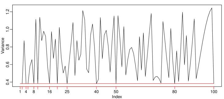
However, the variance of does not converge for arbitrary , e.g., take , , , we calculate and plot the variance in Figure 4. We find that only when is a factor of , that is , is integer, the corresponding variances converges to , for other , the variances do not converge, this is because the ceil of creates an irregular bias , which is of order . If we change the order of in the CLT, the limiting distribution will be either or , which is trivial. Thus we conclude that there are no non-trivial higher-order convergence result for for arbitrary sequence .
For and such that is an irrational number, it is impossible to find such that both and are integers. This means we cannot establish the finite dimensional convergence for , even for a particular convergent sequence of . Therefore we cannot derive any higher-order convergence result for the process .
Appendix S3 Proof in Section 6
First we show a result which controls the difference between the algorithm and the ODE,
Proposition S3.1.
Assume for some , and for fixed , is non-degenerated over the interval , then we have
Proof.
The partial derivative of w.r.t. and are:
| (S3.1) | ||||
When is non-degenerated and continuous over a fixed interval , all eigenvalues of are bounded in . Then and are bounded, and the normal density function is a Lipschitz function of and , that is, there exists , such that,
| (S3.2) |
Moreover, if , then
| (S3.3) | ||||
Now we look at the difference of and between consecutive steps in the algorithm. In the current step, the distribution is denoted by , and in the next step, we take as the minimizer of , then by [38], and , and by taking partial derivative in the JKO scheme, we get
Furthermore, we have
| (S3.4) | ||||
Let , , then , and
| (S3.5) | ||||
Similarly, we have
then if ,
∎
S3.1 Proof of Theorem 6.1
Recall that
Since , we have
| (S3.6) | ||||
then
Similarly,
using Gronwall’s inequality, we can show that
| (S3.7) |
Then by the first line of (S3.6),
| (S3.8) |
For , we can also get
| (S3.9) | ||||
then as , and will converge to the solution to and . By the tightness (S3.7), we can also show the weak convergence result.
Since , we can prove Proposition S3.1 with replaced by . If , by Delta method we have
S3.2 Proof of Theorem 6.2
Given (A7) and , use the same technique in the proof of Theorem 5.1, we can also show:
| (S3.10) |
and
| (S3.11) |
By (S3.10) and (S3.11), we have
Just like (S3.6), we get
| (S3.12) | ||||
Similarly, we have
By Gronwall’s inequality,
| (S3.13) |
Then by (S3.10), (S3.11), (S3.12) and (S3.13),
Then will converge to , similarly we can show converges to .
Since , Proposition S3.1 still holds with , then if , by Delta method we have