Accuracy versus Predominance: Reassessing the validity of the quasi-steady-state approximation

Abstract

The application of the standard quasi-steady-state approximation to the Michaelis–Menten reaction mechanism is a textbook example of biochemical model reduction, derived using singular perturbation theory. However, determining the specific biochemical conditions that dictate the validity of the standard quasi-steady-state approximation remains a challenging endeavor. Emerging research suggests that the accuracy of the standard quasi-steady-state approximation improves as the ratio of the initial enzyme concentration, $e_{0}$, to the Michaelis constant, $K_{M}$, decreases. In this work, we examine this ratio and its implications for the accuracy and validity of the standard quasi-steady-state approximation. Using standard tools from the analysis of ordinary differential equations, we show that while $e_{0}/K_{M}$ provides an indication of the standard quasi-steady-state approximation’s asymptotic accuracy, the sQSSA’s predominance relies on a small ratio of $e_{0}$ to the Van Slyke-Cullen constant, $K$. We conclude that the magnitude of $e_{0}/K$ offers the most accurate measure of the validity of the standard quasi-steady-state approximation.

} }}}

1 Introduction

The Michaelis–Menten (MM) reaction mechanism, a cornerstone of enzyme kinetics, describes the irreversible catalysis of a substrate, $S$, into product, $P$, by an enzyme, $E$:

$$\ce$$

where $C$ represents an enzyme-substrate intermediate complex [1]. The simplest form of the mass action equations modeling the dynamics of the substrate, complex, enzyme, and product concentrations ($s$, $c$, $e$, and $p$, respectively) is a two-dimensional system of ordinary differential equations (ODEs):

$$\dot{s} =-k_{1}(e_{0}-c)s+k_{-1}c,$$ (1a)

$$\dot{c} =\;\;\;k_{1}(e_{0}-c)s-(k_{-1}+k_{2})c,$$ (1b)

with $\dot{e}=-\dot{c}$, $\dot{p}=k_{2}c$, where “$\dot{\phantom{x}}$” denotes differentiation with respect to time, $t$. The constant, $e_{0}$, is the initial enzyme concentration, a conserved quantity.

Closed-form solutions to (1) are unattainable due to quadratic nonlinearities. Consequently, reduced equations approximating the long-time dynamics of (1) are often employed to both elucidate the kinetics of (1) and serve as a forward model for parameter estimation from in vitro progress curve experiments via nonlinear regression [2, 3, 4]. The standard quasi-steady-state approximation (sQSSA) to the mass action equations associated with the MM reaction mechanism is a well-known and extensively studied reduced model in biochemical kinetics [2, 5]. Simply put, the sQSSA is a differential algebraic equation (DAE) that approximates the depletion of substrate:

$$\dot{s}=-\cfrac{k_{2}e_{0}s}{K_{M}+s},\quad c=\cfrac{e_{0}s}{K_{M}+s}$$ (2)

where $K_{M}=(k_{-1}+k_{2})/k_{1}$ is the Michaelis constant and $k_{2}\,e_{0}$ is the limiting rate. The Michaelis constant is composite of the equilibrium constant $K_{S}=k_{-1}/k_{1}$ and the Van Slyke-Cullen constant $K=k_{2}/k_{1}$, and can be expressed as $K_{M}=K_{S}+K$. We assume initial conditions for (1) lie on the s-axis, i.e., $(s,c)(0)=(s_{0},0)$. Under this assumption, we can equip (2) with the initial condition $s(0)=s_{0}$.

Geometric singular perturbation theory provides mathematical justification for (2): with $(s,c)(0)=(s_{0},0)$, the solution to mass action system (1) converges to the DAE (2) in the limit as $e_{0}\to 0$, provided all other parameters, $k_{-1},k_{2}$ and $k_{1}$, are bounded above and below by positive constants [see, e.g. 6, 7]. For further information on geometric singular perturbation theory, see Kaper and Kaper [8], Hek [9], Jones [10] and Wechselberger [11].

While the mathematical rationale behind (2) is well-established, applying (2) presents a challenge: determining how small $e_{0}$ must be to ensure (2) is sufficiently accurate. This assessment is complicated by the relative nature of “small.” $e_{0}$ is only small compared to another quantity, but what is that quantity? Emerging research [see, e.g. 12, 13, 7] suggests that the sQSSA is accurate whenever $e_{0}\ll K_{M}$, or $\varepsilon_{RS}=e_{0}/K_{M}\ll 1$, which we refer to as the Reich-Sel’kov condition [14]. Thus, the “other” quantity is the Michaelis constant, $K_{M}$, and the sQSSA is considered valid – in the sense of accuracy – when the Reich-Sel’kov condition holds.

Beyond accuracy, it is crucial to determine conditions that ensure the predominance of the sQSSA (2). When the reaction unfolds away from the singular limit (i.e., with $0<e_{0}$), multiple reduced models may be accurate. However, it is not obvious that the Reich-Sel’kov condition guarantees that the sQSSA is the predominant reduction. Other reduced models may be more accurate than the sQSSA even when $e_{0}\ll K_{M}$ (see Section 2). Therefore, identifying the most accurate approximation among the available reduced models is essential, and this most accurate model should be labeled as the predominant reduction.

This paper aims to deepen our understanding of the Reich-Sel’kov condition and distinguish between accuracy and predominance concerning the sQSSA (2). To our knowledge, this distinction has not been previously addressed in the literature. Using rigorous phase-plane analysis and methods from ODE analysis, we demonstrate that while the Reich-Sel’kov condition provides a general indication of the sQSSA’s accuracy, it does not ensure its predominance, which requires a more restrictive criterion. We derive this qualifier and challenge the notion that the validity of the sQSSA solely pertains to its accuracy. We argue that validity should encompass both the accuracy and predominance of the sQSSA. In essence, the qualifier establishing the sQSSA’s validity is more restrictive than any previously reported condition.

2 Fenichel Theory, TFPV Theory, and Literature Review

This section reviews Fenichel theory and Tikhonov-Fenichel Parameter Value (TFPV) theory, placing the problem within a precise mathematical context. We also examine recent literature on the validity of the sQSSA (2).

2.1 A brief introduction of Fenichel theory

Geometric singular perturbation theory, also known as Fenichel theory [15, 16], provides the rigorous foundation for deriving the sQSSA. Consider a perturbed dynamical system:

$$\dot{x}=f(x,\varepsilon),\quad f:\mathbb{R}^{n}\times\mathbb{R}\to\mathbb{R}^{n}$$ (3)

where $\varepsilon\in\mathbb{R}$ is a small parameter close to zero. If the set of singularities:

$$S_{0}:=\{x\in\mathbb{R}^{n}:f(x,0)=0\}$$ (4)

is a non-empty $k$-dimensional submanifold of $\mathbb{R}^{n}$ where $0<k<n$, then (3) is singularly perturbed [11]. The rank of the Jacobian with respect to $x$, $D_{1}f(x,0)$, is constant and equal to $n-k$ along $S_{0}$.

2.1.1 Persistence and Flow

A key result from Fenichel theory states that if $S_{0}$ is compact and normally hyperbolic – meaning the $n-k$ non-zero eigenvalues of $D_{1}f(x,0)$ are strictly bounded away from the imaginary axis along $S_{0}$ – then $S_{0}$ persists. This means an invariant manifold, $S_{0}^{\varepsilon}$, exists for $\varepsilon\in[0,\varepsilon_{0})$. Expressing $S_{0}^{\varepsilon}$ as a graph over the first “$k$” coordinates of $x$

$$S_{0}^{\varepsilon}:=\{(z,y,\varepsilon)\in\mathbb{R}^{k}\times\mathbb{R}^{n-k}\times\mathbb{R}:y=h(z,\varepsilon)\},$$ (5)

where $x:=(z,y)$ and $z\in\mathbb{R}^{k},\,y\in\mathbb{R}^{n-k}$, the flow on $S_{0}^{\varepsilon}$ is given by:

$$\dot{z}_{i}=f_{i}(z,h(z,\varepsilon),\varepsilon),\quad 1\leq i\leq k$$ (6)

where the $f_{i}$’s are the component functions of $f$. Equation (6) describes the evolution of $k$-independent variables. The evolution of the remaining $n-k$ variables depends on the evolution of $z$:

$$\dot{y}=D_{1}h(z,\varepsilon)\dot{z},\quad D_{1}h(z,\varepsilon)\in\mathbb{R}^{(n-k)\times k}.$$ (7)

2.1.2 Critical Manifolds and Stability

In singular perturbation theory, the submanifold $S_{0}$ of stationary points is the critical manifold. The persistence of a normally hyperbolic $S_{0}$ asserts the existence of a normally hyperbolic invariant manifold, $S_{0}^{\varepsilon}$, and also the persistence of its stable and unstable manifolds, $W^{s}(S_{0})$ and $W^{u}(S_{0})$. Thus, $S_{0}^{\varepsilon}$ inherits the stability properties as $S_{0}$. If $S_{0}$ is normally hyperbolic and attracting, (6) describes the long-time evolution of (3) because trajectories near $S_{0}^{\varepsilon}$ contract towards it exponentially.

2.1.3 Approximating the Slow Flow

Fenichel’s initial results require explicit knowledge of $S_{0}^{\varepsilon}$, which is often unavailable in practice. To address this, Fenichel [16] proposed a method to approximate the flow in $S_{0}^{\varepsilon}$ without explicitly knowing it. Expanding $f(x,\varepsilon)$ in a Taylor series near $\varepsilon=0$ gives:

$$\dot{x}=f(x,0)+\cfrac{\partial f(x,\varepsilon)}{\partial\varepsilon}\Bigg{|}_{\varepsilon=0}\cdot\varepsilon+\mathcal{O}(\varepsilon^{2})=:f_{0}(x)+\varepsilon f_{1}(x)+\mathcal{O}(\varepsilon^{2}).$$ (8)

If $S_{0}$ is normally hyperbolic and attracting, a splitting exists:

$$T_{x}\mathbb{R}^{n}\cong\mathbb{R}^{n}=\ker D_{1}f(x,0)\oplus\;\text{image}\;D_{1}f(x,0)$$ (9)

for all $x\in S_{0}$, where $T_{x}S_{0}\cong\ker D_{1}f(x,0)$ for all $x\in S_{0}$. Projecting the right-hand side of (8) onto $T_{x}S_{0}$ approximates the flow on $S_{0}^{\varepsilon}$. This projection is achieved using the operator $\pi^{s}:\mathbb{R}^{n}\to\ker D_{1}f(x,0)$; see Goeke and Walcher [17] and Wechselberger [11] for details on the construction of $\pi^{s}$. The resulting $n$-dimensional dynamical system (with “$k$” independent variables) is:

$$x^{\prime}=\pi^{s}f_{1}(x)|_{x\in S_{0}}$$ (10)

where “$\phantom{x}{}^{\prime}$” denotes differentiation with respect to the slow timescale, $\tau=\varepsilon t$. The flow on $S_{0}^{\varepsilon}$ given by (6) converges to (10) as $\varepsilon\to 0$. Equation (10) is referred to as quasi-steady-state approximation (QSSA) in chemical kinetics.

2.1.4 Convergence and Initial Conditions

Solutions to (3) with initial condition $x(0)=(z,y)(0)=(z_{0},y_{0})$ generally do not converge to the solution of (10) with initial condition $z(0)=z_{0}$ unless $z_{0}$ is near $S_{0}$, or $z$ and $y$ are slow and fast coordinates. To ensure convergence, (10) usually requires a modified initial “$\widehat{z}_{0}$”.

2.2 From Theory to Practice: Tikhonov-Fenichel Parameter Values

Traditional methods for putting mass action equations into perturbation form involve scaling and dimensional analysis, which can be unreliable. A more robust approach considers the mass action equations for a general reaction mechanism:

$$\dot{x}=f(x,p),\quad f:\mathbb{R}^{n}\times\mathbb{R}^{m}\to\mathbb{R}^{n}$$ (11)

where “$p$” represents an $m$-tuple of parameters. A point $p^{*}$ in parameter space is a Tikhonov-Fenichel Parameter Value (TFPV) [6, 18] if:

1. The set $S_{0}=\{x\in\mathbb{R}^{n}:f(x,p^{*})=0\}$ is a $k$-dimensional submanifold of $\mathbb{R}^{n}$ with $0<k<n$, and

2. $S_{0}$ is normally hyperbolic.

Expanding $f(x,p)$ near $p^{*}$ in a direction $\rho$, $p=p^{*}+\varepsilon\rho$, gives

$$\dot{x}=f(x,p^{*})+\varepsilon D_{2}f(x,p^{*})\rho,$$ (12)

which matches the form (10). This highlights the need to specify a path in parameter space for taking the limit as $\varepsilon\to 0$ and $p\to p^{*}$.

For the MM system (1), the parameter space is a subset of $\mathbb{R}^{4}_{\geq 0}$ with $p=(e_{0},k_{1},k_{-1},k_{2})^{T}$. Here, $p^{*}:=(0,k_{1},k_{-1},k_{2})^{T}$ is a TFPV if $k_{1}$, $k_{-1}$, $k_{2}$ are bounded by positive constants. When $p=p^{*}$, the critical manifold, $S_{0}$, is the $s$-axis, which is normally hyperbolic and attractive.

To put (1) into perturbation form, we define a curve $\ell(\cdot)$ that passes through $p^{*}$

$$\ell(\varepsilon)=\begin{pmatrix}0\\ k_{1}\\ k_{-1}\\ k_{2}\end{pmatrix}+\varepsilon\begin{pmatrix}\widehat{e}_{0}\\ 0\\ 0\\ 0\end{pmatrix}=p^{*}+\varepsilon\rho$$ (13)

where $e_{0}\mapsto\varepsilon\widehat{e}_{0}$. This effectively equates “$\varepsilon$” with $e_{0}$. The perturbation form of (1) for small $e_{0}$ is

$$\begin{pmatrix}\dot{s}\\ \dot{c}\end{pmatrix}=\begin{pmatrix}(k_{1}s+k_{-1})c\\ -(k_{1}s+k_{-1}+k_{2})c\end{pmatrix}+\varepsilon\widehat{e}_{0}k_{1}s\begin{pmatrix}-1\\ \;\;\;1\end{pmatrix}$$ (14)

Projecting the right hand side of (14) onto $TS_{0}$ yields the sQSSA (2):

$$\begin{pmatrix}\dot{s}\\ \dot{c}\end{pmatrix}=-\cfrac{\varepsilon\widehat{e}_{0}k_{2}s}{K_{M}+s}\begin{pmatrix}1\\ 0\end{pmatrix}\equiv-\cfrac{k_{2}e_{0}s}{K_{M}+s}\begin{pmatrix}1\\ 0\end{pmatrix}.$$ (15)

This derivation implies that the flow on $S_{0}^{\varepsilon}$ converges to (15) as $e_{0}\to 0$, with other parameters fixed and positive. Furthermore, the solution to the first component of (1) also converges to (15) since the initial condition $(s_{0},0)\in S_{0}$.

Other TFPV values exist for (1). For instance, with $p^{*}=(e_{0},k_{1},k_{-1},0)^{T}$, the Fenichel reduction is the slow product QSS reduction:

$$\begin{pmatrix}\dot{s}\\ \dot{c}\end{pmatrix}=-\cfrac{k_{2}e_{0}s(K_{S}+s)}{K_{S}e_{0}+(K_{S}+s)^{2}}\begin{pmatrix}1\\ \cfrac{K_{S}e_{0}-K(K_{S}+s)}{(K_{S}+s)^{2}}\end{pmatrix},$$ (16)

This reduction differs from (15) and will be analyzed in Section 4.

2.3 The Open Problem: Identifying the Predominant Reduction

Just as important as what Fenichel and TFPV theory tell us is what they do not. While the theory indicates that (15) approximates (1) as $e_{0}\to 0$, it does not specify how small $e_{0}$ must be for (15) to be valid in practice, where the singular limit is never truly reached. In other words, how small is small enough?

The size of $e_{0}$ must be considered relative to other parameters. Fenichel theory requires eigenvalue disparity near the critical manifold. For small $e_{0}$, the ratio of slow and fast eigenvalues near $(s,c)=(0,0)$ is:

$$\delta:=\cfrac{e_{0}}{K_{M}}\cdot\cfrac{k_{2}}{k_{-1}+k_{2}}+\mathcal{O}(e_{0}^{2}).$$ (17)

While $\delta\ll 1$ is necessary, it is not sufficient for the accuracy of (15) [12]. For instance, consider the case where $e_{0}=K_{M}$ but $k_{2}\ll k_{-1}$. This scenario renders small $\delta$, but the tangent vector to the graph of the $c$-nullcline at the origin will not align with the slow eigenvector, which is crucial for long-time accuracy. This misalignment can lead to significant errors in the sQSSA approximation, even when $\delta$ appears to indicate otherwise.

The more restrictive condition $e_{0}\ll K_{M}$, introduced in [14], has been rigorously proven sufficient to guarantee the accuracy of the sQSSA [19, 13, 20, 21, 22]. However, this condition does not fully address the issue of predominance. For instance, if $k_{-1}$ is large and $e_{0}$ is reduced such that $k_{1}e_{0}\ll k_{-1}$ (implying $e_{0}\ll K_{M}$), convergence to (15) is not implied. In fact, as $k_{-1}\to\infty$, the resulting singular perturbation problem yields a trivial QSSA: $\dot{s}=\dot{c}=0$ (see E for the formal calculation).

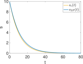
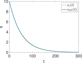
Figure 1: The sQSSA (15) and the slow product QSSA (16) are indistinguishable for large $k_{-1}$. Left: $s_{0}=10$, $c_{0}=0$, $e_{0}=10$, $k_{1}=1$, $k_{-1}=100$, $k_{2}=1.$ Right: $s_{0}=10$, $c_{0}=0$, $e_{0}=10$, $k_{1}=1$, $k_{-1}=500$, $k_{2}=1.$ Substrate depletion over time is shown in both panels. $s_{c}(t)$ is the numerical solution to (15) and $s_{SP}(t)$ is the numerical solution to (16).

This example demonstrates that different TFPVs can share a critical manifold and be close in parameter space. For instance, consider a scenario where $k_{1}e_{0}$ and $k_{2}$ are relatively small compared to $k_{-1}$. In this case, the TFPVs $(0,k_{1},k_{-1},k_{2})^{T}$ or $(e_{0},k_{1},k_{-1},0)^{T}$ could be quite close to each other. Terminating the approach to one TFPV might inadvertently lead to a point in parameter space that is actually closer to another TFPV.

Numerical simulations (Figure 1) illustrate this phenomenon. When $k_{-1}$ is significantly large, the trajectories of the system under the sQSSA (15) and the slow product QSSA (16) become virtually indistinguishable. This makes it challenging to definitively determine which reduction is more accurate or appropriate for the given parameter values.

Moreover, the presence of multiple TFPVs introduces ambiguity in assessing the validity of the sQSSA. For example, if $e_{0}=1$, $k_{1}=0.1$, $k_{-1}=10$, and $k_{2}=0.1$, it is unclear whether the system’s behavior is better approximated by the sQSSA associated with the TFPV $(0,k_{1},k_{-1},k_{2})^{T}$ or the slow product QSSA associated with $(e_{0},k_{1},k_{-1},0)^{T}$. This ambiguity arises because the parameter values do not fall neatly within the domain of a single TFPV, making it difficult to determine which reduction provides the most accurate representation of the system dynamics. Determining proximity to different TFPVs is challenging due to the different units of the parameters. A dimensionless indicator is needed.

The fact that the magnitude of $e_{0}/K_{M}$ alone does not ensure the sQSSA (15) is the predominant reduction is a consequence of having to always operate away from the singular limit in a large parameter space. This naturally leads to the question: does there exist a dimensionless parameter whose magnitude not only ensures the accuracy of the sQSSA (2) but also its predominance among other known QSSAs? In other words, can we define a more comprehensive and robust notion of “validity” that encompasses both accuracy and predominance?

3 Anti-funnels and the Slow Invariant Manifold

As discussed in Section 2, a central challenge in applying Fenichel theory to the MM system is the potential ambiguity arising from different TFPVs sharing the same critical manifold. This can lead to uncertainty about the validity of a specific reduction away from the singular limit. To address this, we turn to qualitative methods that allow us to determine the location of the slow manifold, $S_{0}^{\varepsilon}$, relative to known curves in the phase-plane. This section introduces the anti-funnel theorem, adapted from Hubbard and West [23] and following the approach of Calder and Siegel [24]. We outline a strategy to determine when the sQSSA (2) is not only accurate but also predominant.

Definition 1.

Fences and anti-funnels. Consider the first-order differential equation $y^{\prime}=f(x,y)$ over the interval $x\in I=[a,b)$ where $a<b\leq\infty$ and “$\phantom{x}{}^{\prime}$” denotes differentiation with respect to $x$. Let $\alpha$ and $\beta$ be continuously-differentiable functions that satisfy

$$\alpha^{\prime}(x)\leq f(x,\alpha(x))\;\text{and}\;f(x,\beta(x))\leq\beta^{\prime}(x)$$ (18)

for all $x\in I$.

• The curve $\alpha$ is a lower fence and the curve $\beta$ is an upper fence.

• The lower and upper fences are strong fences if the respective inequalities are always strict.

• The set

  $$\Gamma:=\{(x,y)\;:\;x\in I,\;\beta(x)\leq y\leq\alpha(x)\}$$ (19)

  is called an anti-funnel if

  $$\beta(x)<\alpha(x)\;\;\text{for all}\;\;x\in I.$$

• The anti-funnel is narrowing if

  $$\lim\limits_{x\rightarrow b^{-}}|\alpha(x)-\beta(x)|=0.$$ (20)

Theorem 1.

Anti-funnel Theorem [23]. Consider the first-order differential equation $y^{\prime}=f(x,y)$ over the interval $I=[a,b)$ where $a<b\leq\infty$. If $\Gamma$ is an anti-funnel with a strong lower fence, $\alpha$, and a strong upper fence, $\beta$, then there exists a solution $y(x)$ to the differential equation such that

$$\beta(x)<y(x)<\alpha(x)\;\;\text{for all}\;\;x\in I.$$ (21)

Furthermore, if $\Gamma$ is narrowing and $\frac{\partial f}{\partial y}(x,y)\geq 0$ in $\Gamma$, then the solution $y(x)$ is unique.

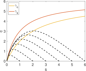
Figure 2: The region, $\Gamma$, between the horizontal nullcline and the vertical nullcline curves is a trapping region on the phase plane. The numerical solutions to the mass action equations (1) for several initial conditions are denoted by black dashed lines. $s_{0}\in\{1,2,3,4,5,6\}$, $c_{0}=0$, $e_{0}=6$, $k_{1}=1$, $k_{-1}=1$, $k_{2}=1.$ The numerical solution of trajectories start on the $s$-axis and eventually enter $\Gamma$.

For the MM equations (1), we have:

$$\frac{\mathrm{d}c}{\mathrm{d}s}=-\cfrac{e_{0}s-(K_{M}+s)c}{e_{0}s-(K_{S}+s)c}=:f(c,s).$$ (22)

The distinguished solution to (22), “$c=y(s)$”, satisfying (21) represents the slow manifold, $S_{0}^{\varepsilon}$. The challenge lies in finding suitable lower and upper fences, $\alpha(s)$ and $\beta(s)$.

A natural choice for the upper fence is the $c$-nullcline, $\gamma_{c}$, given by:

$$\text{Graph}(\gamma_{c})=\{(s,c)\in\mathbb{R}^{2}:c=e_{0}s/(K_{M}+s)\}$$ (23)

Considering the biochemically relevant portion of $\mathbb{R}^{2}$, we focus on $\text{Graph}(\gamma_{c})\cap\mathbb{R}^{2}_{\geq 0}$. This choice is advantageous because it represents the quasi-steady-state variety corresponding to the standard reduction (2), and all phase-plane trajectories starting on the s-axis eventually cross it (see Calder and Siegel [24] and Noethen and Walcher [25] for a proof of this statement).

The set $\Gamma$ enclosed between the $c$-nullcline and the $s$-nullcline, $\gamma_{s}$, is positively invariant:

$$\Gamma:=\{(s,c)\in\mathbb{R}^{2}_{\geq 0}\;:\;\gamma_{c}(s)\leq c\leq\gamma_{s}(s)\}$$ (24)

Once a trajectory enters $\Gamma$, it remains within $\Gamma$ as $t\to\infty$. (see Calder and Siegel [24] and Noethen and Walcher [25] for a detailed proof). Figure 2 illustrates this behavior.

Constructing a suitable lower fence requires more analysis. The stationary point $(s,c)=(0,0)$ is a node with eigenvalues $\lambda_{-}<\lambda_{+}<0$:

$$\lambda_{\pm}=\cfrac{k_{1}}{2}(K_{M}+e_{0})\left(-1\pm\sqrt{1-\cfrac{4Ke_{0}}{(K_{M}+e_{0})^{2}}}\right).$$ (25)

Under timescale separation in which

$$\cfrac{Ke_{0}}{(K_{M}+e_{0})^{2}}\ll 1/4,$$ (26)

trajectories eventually approach the stationary point along the slow eigenvector, $v^{+}$, spanning the one-dimensional subspace:

$$T_{0}S_{0}^{\varepsilon}=\text{span}(v^{+})=\{(s,c)\in\mathbb{R}^{2}:c=ms\},$$ (27)

with slope $m$:

$$m=\frac{1}{2k_{-1}}\left(-k_{-1}-k_{2}+k_{1}e_{0}+\sqrt{(k_{-1}+k_{2}+k_{1}e_{0})^{2}-4k_{1}k_{2}e_{0}}\right).$$ (28)

Calder and Siegel [24] leverage this property and define the lower fence:

$$\alpha_{cs}(s):=\cfrac{me_{0}s}{e_{0}+ms},$$ (29)

and prove that $S_{0}^{\varepsilon}$ lies between $\gamma_{c}(s)$ and $\alpha_{cs}(s)$. Notably, the graph of $\alpha_{cs}$ lies below that of $\gamma_{s}$. By proving that

$$\Gamma_{cs}:=\{(s,c)\;:\;s\in I,\gamma_{c}(s)\leq c\leq\alpha_{cs}(s)\}$$ (30)

is a narrowing anti-funnel, Calder and Siegel [24] prove that the distinguished slow manifold, $S_{0}^{\varepsilon}$, also lies in $\Gamma$, the region contained between the $c$- and $s$-nullcline.

A key feature of (29) is $\alpha_{cs}^{\prime}(0)=m$. This leads to highly accurate reduced equation for $\dot{s}$ near the stationary point:

$$\dot{s}=-\cfrac{e_{0}s}{e_{0}+ms}\cdot(k_{1}e_{0}-k_{-1}m).$$ (31)

Despite its advantages, this approach has limitations. First, the reduction (31) may be unreliable away from the stationary point, even when $\lambda_{-}\ll\lambda_{+}<0$ (see  Eilertsen et al. [26]). Second, the anti-funnel construction leads to the following:

Proposition 1.

For (1) with initial condition $(s,c)(0)=(s_{0},0)$, let $t=t_{\rm cross}$ be the time the trajectory crosses the upper fence $c=\gamma_{c}(s)$. Then, the bound

$$-\cfrac{k_{2}e_{0}s}{K_{M}+s}\leq\dot{s}\leq-\cfrac{e_{0}s}{e_{0}+ms}\cdot(k_{1}e_{0}-k_{-1}m)$$ (32)

holds for all $t\geq t_{\rm cross}$.

Proof.

Since $\Gamma_{cs}$ is a narrowing anti-funnel, $S_{0}^{\varepsilon}$ lies between the graphs of $\alpha_{cs}(s)$ and $\gamma_{c}(s)$. As $S_{0}^{\varepsilon}$ is invariant, any trajectory entering $\Gamma_{cs}$ cannot cross it. Therefore, $\beta(s)\leq c\leq\alpha_{cs}(s)$ holds for all $t\geq t_{\rm cross}$ since $\Gamma$ is positively invariant and $\Gamma_{cs}\subset\Gamma$. With $\dot{s}=-k_{1}e_{0}s+k_{1}(K_{S}+s)c$, it follows that

$$-k_{1}e_{0}s+k_{1}(K_{S}+s)\gamma_{c}(s)\leq\dot{s}\leq-k_{1}e_{0}s+k_{1}(K_{S}+s)\alpha_{cs}(s)$$

proving the assertion. ∎

While the upper bound in (32) is sharper than $\dot{s}\leq 0$, extracting quantitative information about the sQSSA’s accuracy and dimensionless parameters like $\varepsilon_{RS}=e_{0}/K_{M}$ from (32) is not straightforward.

The goal is to define an anti-funnel with fences that provide both qualitative and quantitative information about $S_{0}^{\varepsilon}$ and the error for a given QSSA. By “trapping” $S_{0}^{\varepsilon}$ between suitable upper and lower fences that form narrowing anti-funnels, we can derive qualifiers that determine the accuracy and predominance of various QSSAs.

4 Trapping the Slow Manifold: The Standard QSSA

As stated in Section 3, our strategy is to construct upper and lower fences that form a narrowing anti-funnel. This raises the question: How do we construct suitable fences? One approach is approximating the slow manifold, $S_{0}^{\varepsilon}$, via perturbation expansion

$$S_{0}^{\varepsilon}=h_{0}(s)+\varepsilon h_{1}(s)+\varepsilon^{2}h_{2}(s)+\mathcal{O}(\varepsilon^{2}).$$ (33)

Insertion of (33) into the invariance equation results in a regular perturbation problem. However, the coefficients in (33) depend on $\varepsilon$, which in turn depends on a specific TFPV. Since we aim for general error bounds, we need fences that are not heavily $\varepsilon$-dependent.

An alternative approach involves combining quantitative reasoning with creative insights. Kumar and Josić [27] sought to approximate the flow on $S_{0}^{\varepsilon}$ for small $k_{2}$ ($k_{2}\mapsto\varepsilon\widehat{k}_{2}$). They reasoned that

$$c=\cfrac{e_{0}s}{K_{M}+s}$$ (34)

is a good approximation to $S_{0}^{\varepsilon}$ when $k_{2}$ is small. Under this assumption, the flow of $c$ on $S_{0}^{\varepsilon}$ is approximately:

$$\dot{c}\approx\cfrac{{\rm d}}{{\rm d}s}\left(\cfrac{e_{0}s}{K_{M}+s}\right)\dot{s}=\cfrac{K_{M}e_{0}}{(K_{M}+s)^{2}}\cdot\dot{s}.$$ (35)

Substituting (35) and (34) into the conservation law, $\dot{s}+\dot{c}+k_{2}c=0$, and solving for $\dot{s}$ yields:

$$\dot{s}=-\frac{k_{2}e_{0}s(K_{M}+s)}{K_{M}e_{0}+(K_{M}+s)^{2}}.$$ (36)

This reduction is significant for two reasons. First, it effectively captures the Fenichel reduction for this scenario (compare to (16) with small $k_{2}$). Second, the graph of $\gamma(s)$, where

$$\gamma:s\mapsto\frac{e_{0}s}{K_{S}+s}-\frac{k_{2}e_{0}s(K_{M}+s)}{k_{1}(K_{S}+s)(K_{M}e_{0}+(K_{M}+s)^{2})},$$ (37)

is an excellent candidate for an appropriate anti-funnel fence.

Figure 3: The region between the horizontal nullcline curve $\gamma_{c}(s)$ and the curve $\gamma(s)$ is a trapping region on the phase plane. The numerical solutions to the mass action equations (1) for several initial conditions are denoted by black dashed lines. $s_{0}\in\{1,2,3,4,5,6\}$, $c_{0}=0$, $e_{0}=6$, $k_{1}=1$, $k_{-1}=1$, $k_{2}=1.$

As shown in Figure 3, $\gamma_{c},\gamma_{s}$ and $\gamma$ are strictly increasing, with $\gamma_{c}<\gamma<\gamma_{s}$ for all $s>0$. The set contained between the graphs of $\gamma_{c}$ and $\gamma$ is positively invariant:

$$\Gamma_{0}:=\{(s,c)\in\mathbb{R}^{2}_{\geq 0}\;:\;\gamma_{c}(s)\leq c\leq\gamma(s)\}$$ (38)

Let $t_{\rm cross}$ be the time a trajectory crosses the $c$-nullcline, as established in [25, 24]. Then, $(s,c)(t)\in\Gamma_{0}$ for all $t\geq t_{\rm cross}$. Importantly:

Theorem 2.

For the differential equation (22), $\Gamma_{0}$ is a positively invariant, narrowing anti-funnel containing a unique slow manifold, $S_{0}^{\varepsilon}$.

Proof.

To prove $\Gamma_{0}$ is positively invariant, we show that the vector field for (1) points inwards at the boundary curves:

$$\dot{c}(s,\gamma(s))\;-\gamma^{\prime}(s)\dot{s}(s,\gamma(s))\;<0,$$ (39a)

$$\dot{c}(s,\gamma_{c}(s))-\gamma_{c}^{\prime}(s)\dot{s}(s,\gamma_{c}(s))>0.$$ (39b)

See B for details. Positive invariance implies trajectories entering $\Gamma_{0}$ remain within. Calder and Siegel [24] prove that for solutions initializing on the $s$-axis, there exists a $t_{\rm cross}>0$ at which they enter $\Gamma_{0}$ by crossing $\gamma_{c}$.

From (39), $\gamma$ and $\gamma_{c}$ are strong lower and upper fences, respectively, with $\gamma(s)>\gamma_{c}(s)$ for $s>0$. Furthermore,

$$\lim\limits_{s\rightarrow\infty}|\gamma(s)-\gamma_{c}(s)|=0\quad\text{and}\quad\frac{\partial f}{\partial c}(c,s)\geq 0$$ (40)

in $\Gamma_{0}$. The assertion follows from Theorem  1. ∎

Theorem 2 establishes that $\Gamma_{0}$ contains the slow manifold $S_{0}^{\varepsilon}$, independent of any specific perturbation scenario. This allows us to extract qualitative and quantitative information about the accuracy of a QSSA and assess predominance when multiple TFPVs are close.

The rest of this section is organized as follows. In Section 4.1, we use the improved trapping region to derive a quantitative error estimate for the sQSS approximation and recover the Reich-Sel’kov condition. In Section 4.2, we explore the conditions where both the sQSS and reverse QSS reductions are valid, examining their validity as we move away from the Reich-Sel’kov condition.

4.1 Accuracy of the Standard QSSA

To leverage $\Gamma_{0}$’s properties, we introduce sharp bounds on the substrate depletion for $t\geq t_{\rm cross}$, representing the slow regime.

Proposition 2.

For system (1) with initial condition $(s,c)(0)=(s_{0},0)$, the bound

$$-\frac{k_{2}e_{0}s}{K_{M}+s}\leq\dot{s}\leq-\frac{k_{2}e_{0}s(K_{M}+s)}{K_{M}e_{0}+(K_{M}+s)^{2}}$$ (41)

holds for all $t\geq t_{\rm cross}$.

Proof.

The proof follows from the construction of $\Gamma_{0}$ and substituting $\gamma_{c}(s)\leq c\leq\gamma(s)$ into (1a). ∎

Since the LHS of (41) is the sQSSA for substrate depletion, the design of $\Gamma_{0}$ suggests that the sQSSA performs well when $\gamma$ and $\gamma_{c}$ are close. Rewriting (41) as:

$$-\frac{k_{2}e_{0}s}{K_{M}+s}\leq\dot{s}\leq-\frac{k_{2}e_{0}s}{K_{M}+s}\left(\frac{1}{1+\varphi(s)}\right),\quad\varphi(s)=\cfrac{K_{M}e_{0}}{(K_{M}+s)^{2}}$$ (42)

we see that, for any subinterval $\ell\subset[0,s_{0}]$,

$$-\frac{k_{2}e_{0}s}{K_{M}+s}\leq\dot{s}\leq-\frac{k_{2}e_{0}s}{K_{M}+s}\left(\frac{1}{1+\displaystyle\max_{s\in\ell}\varphi(s)}\right),\quad t_{\rm cross}\leq t.$$ (43)

Since

$$\max_{0\leq s\leq s_{0}}\varphi(s)=\cfrac{e_{0}}{K_{M}}=\varepsilon_{RS},$$ (44)

we have:

$$-\frac{k_{2}e_{0}s}{K_{M}+s}\leq\dot{s}\leq-\frac{k_{2}e_{0}s}{K_{M}+s}\cdot\sum_{j=0}^{\infty}(-1)^{j}\varepsilon_{RS}^{j},\quad t_{\rm cross}\leq t,\quad\varepsilon_{RS}<1.$$ (45)

This analysis has several significant consequences. First, we have established the sQSSA’s asymptotic dependency on $\varepsilon_{RS}$ without relying on non-dimensionalization, unlike traditional methods [see 28, 14, 29, among others]. This is advantageous due to the non-uniqueness of non-dimensionalization, which can lead to different “small parameters” [28, 14, 30]. Second, the bound (45) is more aesthetic than the estimate in Eilertsen et al. [13]:

$$-\frac{k_{2}e_{0}s}{K_{M}+s}\leq\dot{s}\leq-(1-m)\frac{k_{2}e_{0}s}{K_{M}+s},\quad t_{\rm cross}\leq t,$$ (46)

where “$m$” is the slope of the slow tangent vector, $v^{+}$.

Third, and this is somewhat unexpected, we gain more information about the approximation error of the flow on $S_{0}^{\varepsilon}$ from $\varphi(s)$ than from $m$. From (42), the sQSSA approximates the flow on $S_{0}^{\varepsilon}$ well in the regions where:

$$K_{M}e_{0}\ll(K_{M}+s)^{2},$$ (47)

even if $\varepsilon_{RS}\sim 1$. In particular, the sQSSA is a good approximation in regions where:

$$\max\{K_{M},e_{0}\}\ll s.$$ (48)

This relates to the validity of the reverse quasi-steady-state approximation (rQSSA), which operates in high enzyme concentrations. To revisit the sQSSA’s predominance, we examine the rQSSA’s validity and investigate any overlap in their conditions.

4.2 Validity of the sQSSA for High Enzyme Concentrations

Equation (42) implies that the sQSSA is an excellent approximation to the flow on $S_{0}^{\varepsilon}$ when $K_{M}\ll s$ and $e_{0}\lesssim s$. In this region, the graphs of the $c$-nullcline and $\gamma(s)$ approach their horizontal asymptote, $c=e_{0}$, reflected in $\varphi(s)\to 0$ as $s\to\infty$. The slow manifold, $S_{0}^{\varepsilon}$, is nearly horizontal implying $\dot{c}\approx 0$ on $S_{0}^{\varepsilon}$ even for larger $\varepsilon_{RS}$.

Two singular perturbation scenarios lead to a nearly horizontal slow manifold: the sQSSA, where the slow manifold coalesces with the $s$-axis as $k_{1}e_{0}\to 0$, and the rQSSA, coinciding with small $k_{-1}$ and small $k_{2}$:

$$\dot{s} =-k_{1}(e_{0}-c)s+\varepsilon\widehat{k}_{-1}c,$$ (49a)

$$\dot{c} =\;\;\;k_{1}(e_{0}-c)s-\varepsilon\widehat{k}_{-1}-\varepsilon\widehat{k}_{2}.$$ (49b)

In the rQSSA scenario, the set of stationary points in the singular limit is not a submanifold of $\mathbb{R}^{2}$:

$$S_{0}=S_{0}^{(1)}\cup S_{0}^{(2)}$$

where

$$S_{0}^{(1)} =\{(s,c)\in\mathbb{R}^{2}_{\geq 0}:s=0\;\&\;0\leq c\leq e_{0}-\zeta_{1}\},\quad 0<\zeta_{1}<e_{0},$$ (50a)

$$S_{0}^{(2)} =\{(s,c)\in\mathbb{R}^{2}_{\geq 0}:c=e_{0}\;\&\;\zeta_{2}\leq s\leq s_{0}\},\;\qquad 0<\zeta_{2}<s_{0}.$$ (50b)

Classical Fenichel theory does not apply to the entire set, but it applies to specific compact submanifolds. The resulting Fenichel reduction via projection onto $TS_{0}^{(2)}$ is:

$$\dot{s} =-k_{2}e_{0},$$ (51a)

$$\dot{c} =0.$$ (51b)

Likewise, the Fenichel reduction obtained via projection onto $TS_{0}^{(1)}$ is:

$$\dot{s} =0,$$ (52a)

$$\dot{c} =-k_{2}c.$$ (52b)

In the rQSSA, trajectories initially approach the line $c=e_{0}$ and stay close until reaching the vicinity of the transcritical bifurcation point, $(s,c)=(0,e_{0})$. Near this point, trajectories approach $(0,0)$ as $t\to\infty$; however, the slow eigenvector in this scenario is nearly indistinguishable from the $c$-axis (and in fact aligns with the $c$-axis in the singular limit).

The rQSSA’s long-time validity requires $\varepsilon_{RS}^{-1}\ll 1$, while the sQSSA’s long-time validity requires $\varepsilon_{RS}\ll 1$ [19]. However, through comparison, the sQSSA with (51) reveals that they are practically indistinguishable when $K_{M}\ll e_{0}\lesssim s$. Thus, the sQSSA can approximate the flow on $S_{0}^{\varepsilon}$ to the right of the bifurcation point, extending its validity beyond the Reich-Sel’kov parameter.

A natural question is: If we use the sQSSA to approximate the flow on $S_{0}^{\varepsilon}$ to the right of the bifurcation instead of (51), how reliable is it in an asymptotic sense? Since $S_{0}^{\varepsilon}$ lies within $\Gamma_{0}$ when $0<\varepsilon$, we can get a rough answer. Assuming $\varepsilon_{RS}^{-1}\ll 1$ and considering $s\in[e_{0},s_{0}]$, it follows from (42) that, for $t\geq t_{\rm cross}$,

$$-\cfrac{k_{2}e_{0}s}{K_{M}+s}\leq\dot{s} \leq-\cfrac{k_{2}e_{0}s}{K_{M}+s}\left(\cfrac{1}{1+\displaystyle\max_{s\in[e_{0},s_{0}]}\varphi(s)}\right)$$ (53)

$$=-\cfrac{k_{2}e_{0}s}{K_{M}+s}\left(\cfrac{1}{1+\displaystyle\mu}\right),\quad\mu:=\cfrac{\varepsilon_{RS}}{(1+\varepsilon_{RS})^{2}}<\varepsilon_{RS}^{-1}$$

$$\leq-\cfrac{k_{2}e_{0}s}{K_{M}+s}\left(\cfrac{1}{1+\varepsilon_{RS}^{-1}}\right)$$

$$=-\cfrac{k_{2}e_{0}s}{K_{M}+s}\cdot\sum_{j=0}^{\infty}(-1)^{j}\varepsilon_{RS}^{-j},\quad 1<\varepsilon_{RS}.$$

The bound (53) implies the sQSSA is a good approximation when $\varepsilon_{RS}^{-1}\ll 1$ and $e_{0}\lesssim s$, improving as $e_{0}/s\to 0$.

While the sQSSA approximates the flow on $S_{0}^{\varepsilon}$ well when $\varepsilon_{RS}^{-1}\ll 1$ and $e_{0}\lesssim s$, it cannot be equipped with $s_{0}$ as the initial substrate concentration in the rQSSA scenario. If the initial condition is $(s,c)(0)=(s_{0},0)$, with $e_{0}<s_{0}$, Fenichel theory dictates that the reduction (51) should be equipped with $(s,c)=(s_{0}-e_{0},e_{0}).$ This extends to the sQSSA if used to approximate the flow on $S_{0}^{\varepsilon}$ to the right of the bifurcation point when $\varepsilon_{RS}^{-1}\ll 1$.

The existence of multiple accurate QSS reductions under the same conditions necessitates evaluating which QSSA is predominant. To truly verify the standard-QSS reduction’s applicability, we must explore other QSS reductions near the sQSS curve in the phase-plane. As noted in Section 3, in scenarios like large $k_{-1}$, the sQSSA (15) and the slow product QSSA (16) are indistinguishable. To find the most accurate reduced system and its validity conditions, we next investigate the slow manifold’s location relative to the (algebraic) variety that generates the slow product QSS reduction (16).

5 Trapping the Slow Manifold: The Slow Product QSSA

This section defines a new upper fence and anti-funnel for the slow manifold using the slow product QSS curve under specific parametric restrictions. We compare this to previous results to assess the approximation accuracy of the sQSSA (15) and the slow product QSSA (16), revisiting the Reich-Sel’kov condition and investigating whether it ensures the predominance of the sQSSA.

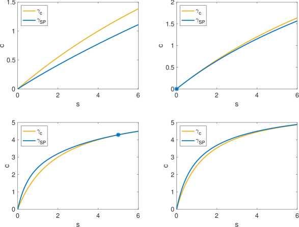
Figure 4: The slow product QSS curve $\gamma_{SP}$ lies above the horizontal nullcline $\gamma_{c}$ for $s<s^{*}$ (55) in the phase plane. Top Left ($k_{2}>e_{0}k_{1}$): $k_{1}=0.1$, $k_{2}=1$, $k_{-1}=1$, $e_{0}=6$, $s^{*}=-4$. Top Right ($k_{2}=e_{0}k_{1}$): $k_{1}=0.1$, $k_{2}=0.6$, $k_{-1}=1$, $e_{0}=6$, $s^{*}=0$. Bottom Left ($k_{2}<e_{0}k_{1}$): $k_{1}=1$, $k_{2}=1$, $k_{-1}=1$, $e_{0}=6$, $s^{*}=5$. Bottom Right ($k_{2}<e_{0}k_{1}$): $k_{1}=1$, $k_{2}=0.4$, $k_{-1}=1$, $e_{0}=6$, $s^{*}=14$.

The slow product QSS reduction (16), derived from Fenichel theory for small $k_{2}$, corresponds to the QSS curve

$$c=\gamma_{SP}(s):=\frac{e_{0}s}{K_{S}+s}-\frac{k_{2}e_{0}s}{k_{1}(K_{S}e_{0}+(K_{S}+s)^{2})}.$$ (54)

This closely resembles the curve $\gamma(s)$. In Section 4.1, we established that the slow manifold lies between $\gamma(s)$ and $\gamma_{c}(s)$. Now, we explore how the slow product QSS variety fits into these findings and the insights its location provides concerning the sQSSA’s validity and predominance.

In the phase plane, $\gamma_{SP}(s)$ lies above the horizontal nullcline $\gamma_{c}(s)$ for $s<s^{*}$ where

$$s^{*}=\frac{k_{-1}e_{0}}{k_{2}}-\frac{k_{-1}}{k_{1}}=\frac{k_{-1}}{k_{2}}(e_{0}-K)$$ (55)

is their intersection point for substrate concentration. We are primarily interested in cases where $s^{*}$ is positive, placing the intersection within the first quadrant. When $s^{*}$ is negative, or equivalently, when

$$e_{0}<K,$$ (56)

the slow manifold crosses the sQSS variety, and the sQSSA is the best known reduction.

However, as $e_{0}$ increases, $s^{*}$ shifts to the right. Figure 4 shows how the curves’ positions change with parameter values. When $e_{0}>K$, the intersection point lies in the first quadrant and $\gamma_{SP}(s)\geq\gamma_{c}(s)$ for $0\leq s\leq s^{*}$. Also, $\gamma_{SP}(s)\leq\gamma(s)$ for all $s\geq 0$. Thus, the slow product QSS curve lies within $\Gamma_{0}$ for a significant portion of the phase plane. This raises the questions: Do solutions cross $\gamma_{SP}(s)$ after crossing $\gamma_{c}(s)$ under any parametric conditions? If so, can we locate the slow manifold more precisely?

Numerical evidence suggests this is possible, with solutions lying closer to the slow product QSS curve in the steady-state regime (see Figure 5). Interestingly, the parametric conditions for this also ensure the slow-product QSS reduction’s dominance over the sQSS reduction, aligning with our overall goal.

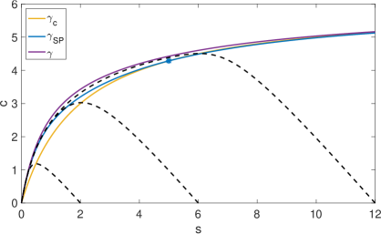
Figure 5: The region between the slow product QSS curve $\gamma_{SP}(s)$ and the curve $\gamma(s)$ is a trapping region for solutions in the phase plane when $e_{0}<8K_{S}$. The intersection point of $\gamma_{SP}$ and $\gamma_{c}$, $s^{*}$, is denoted by the blue star. The numerical solutions to the mass action equations (1) for several initial conditions are denoted by black dashed lines. $s_{0}\in\{2,6,12\}$, $c_{0}=0$, $e_{0}=6$, $k_{1}=1$, $k_{-1}=1$, $k_{2}=1.$

Our main results establish the conditions for positive invariance of the set bordered by the graphs of $\gamma_{SP}(s)$ and $\gamma(s)$:

$$\Gamma_{SP}:=\left\{(s,c)\in\mathbb{R}^{2}_{\geq 0}\;:\;\;\gamma_{SP}(s)\leq c\leq\gamma(s)\right\},$$ (57)

and show that all solutions eventually cross $\gamma_{SP}(s)$ under those conditions.

Theorem 3.

For a solution $(s,c)(t)$ to (1) with initial conditions $(s,c)(0)=(s_{0},0)$. If $e_{0}<8K_{S}$, then there exists a $t_{\rm cross\_sp}>0$ at which the trajectory crosses $\gamma_{SP}(s)$, and

$$(s,c)(t)\in\Gamma_{SP},\quad\forall\;t\geq t_{\rm cross\_sp}.$$ (58)

Proof.

To establish positive invariance, we show that the vector field at the boundary curve $\gamma_{SP}$ points towards $\Gamma_{SP}$ when $e_{0}<8K_{S}$:

$$\dot{c}(s,\gamma_{SP}(s))-\gamma_{SP}^{\prime}(s)\dot{s}(s,\gamma_{SP}(s))>0$$ (59)

See C for details. Combining this with (39a) ensures solutions entering $\Gamma_{SP}$ remain within.

We also show that solutions beginning outside $\Gamma_{SP}$ eventually enter it. In contradiction, assume that a solution starting at $(s_{0},0)$ converges to the stationary point $(0,0)$ without entering $\Gamma_{SP}$. Then, the slope of the tangent to $c=\gamma_{SP}(s)$ at $s=0$ should be greater than $m$ (28). However, we show that

$$\gamma_{SP}^{\prime}(0)<m$$ (60)

always holds, where:

$$\gamma_{SP}^{\prime}(0)=\frac{k_{1}e_{0}}{k_{-1}}-\frac{k_{2}e_{0}}{k_{-1}(K_{S}+e_{0})}.$$ (61)

When $e_{0}<K$, $\gamma^{\prime}_{SP}(0)<\gamma^{\prime}_{c}(0)$ holds, and Theorem 2 implies $\gamma^{\prime}_{c}(0)<m$, demonstrating $\gamma^{\prime}_{SP}(0)<m$. For $e_{0}>K$, see D for proof of (60). Thus, our assumption is false, and a $t_{\rm cross\_sp}>0$ exists when the trajectory crosses $\gamma_{SP}(s)$. The proof is complete by combining the two arguments. ∎

The primary benefit of establishing the positive invariance of $\Gamma_{SP}$ is that it allows for a more precise localization of the slow manifold.

Theorem 4.

If $e_{0}<8K_{S}$, then for the differential equation (22), $\Gamma_{SP}$ is a positively invariant, narrowing anti-funnel within which there exists a unique slow manifold, $S_{0}^{\varepsilon}$.

Proof.

Inequality (59) ensures $c=\gamma_{SP}(s)$ is a strong upper fence for (22) when $e_{0}<8K_{S}$. It is verifiable that $\gamma(s)>\gamma_{SP}(s)$ for $s>0$ and:

$$\lim\limits_{s\rightarrow\infty}|\gamma(s)-\gamma_{SP}(s)|=0$$ (62)

implying $\Gamma_{SP}$ (38) is a narrowing anti-funnel for $e_{0}<8K_{S}$. Further,

$$\cfrac{\partial f}{\partial c}(c,s)\geq 0$$ (63)

in $\Gamma_{SP}$, and the claim follows from Theorem 1. ∎

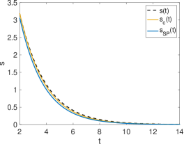
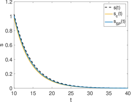
Figure 6: The condition $e_{0}<K$ ensures that the sQSSA provides a better approximation than the slow product QSSA under the Reich-Sel’kov condition. $e_{0}\ll K_{M}$ is satisfied in both panels. Left ($e_{0}<K$): $s_{0}=9$, $c_{0}=0$, $e_{0}=6$, $k_{1}=1$, $k_{-1}=100$, $k_{2}=10.$ Right ($e_{0}>K$): $s_{0}=9$, $c_{0}=0$, $e_{0}=6$, $k_{1}=1$, $k_{-1}=100$, $k_{2}=4$. Substrate depletion over time is shown in both panels. The numerical solution to the mass action equations (1) is denoted by black dashed lines. $s_{c}(t)$ is the numerical solution to (15) and $s_{SP}(t)$ is the numerical solution to (16).

The slow manifold is contained within $\Gamma_{SP}$ when $e_{0}<8K_{S}$. While this condition might seem restrictive, it connects directly to the sQSSA’s validity analysis. We show that the slow manifold lies closer to the slow product QSS curve than the sQSS curve when $e_{0}<8K_{S}$. The remaining task is to analyze the implications of this location.

5.1 Revisiting the Reich-Sel’kov Condition

The Reich-Sel’kov qualifier ensures the sQSS reduction’s accuracy, as validated in Section 4 using the novel anti-funnel (2). Our analysis shows that the sQSSA is the best known approximation to the slow manifold under most parametric scenarios. For instance, recall the intersection point (55). When $e_{0}<K$, the intersection is inconsequential. Consequently, when the Reich-Sel’kov condition $e_{0}\ll K_{M}$ is combined with $e_{0}<K$, the sQSSA is the predominant approximation.

What happens when $e_{0}\ll K_{M}$, $e_{0}\ll K_{S}$ (ensuring $e_{0}<8K_{S}$), but $e_{0}>K$? Theorem 3 implies that trajectories lie closer to $\gamma_{SP}$ than to $\gamma_{c}$ for a significant portion of the slow dynamics (see Figure 5), and therefore

$${-\cfrac{k_{2}e_{0}s}{K_{M}+s}\leq-\cfrac{k_{2}e_{0}s(K_{S}+s)}{K_{S}e_{0}+(K_{S}+s)^{2}}\leq\dot{s}\leq-\cfrac{k_{2}e_{0}s(K_{M}+s)}{K_{M}e_{0}+(K_{M}+s)^{2}}}$$ (64)

after the trajectories cross $\gamma_{SP}$ and $s\leq s^{*}$. Moreover, we know that the slope $m$ of the linear approximation is greater than the slope of the tangent to $\gamma_{SP}$ at the origin (60) and $\gamma_{SP}^{\prime}(0)>\gamma_{c}^{\prime}(0)$ whenever $e_{0}>K$. Thus, the approximation errors near the stationary point follow:

$$m-\gamma_{SP}^{\prime}(0)<m-\gamma_{c}^{\prime}(0)$$ (65)

when $e_{0}>K$. Consequently, complementing the Reich-Sel’kov condition with the stronger condition $e_{0}<K$ is necessary to guarantee that the sQSS is indeed the predominant quasi-steady-state approximation of the MM reaction mechanism, and this may be relevant in the context of the inverse problem where parameters are estimated at low substrate concentration [3]: If $e_{0}>K$, using the slow product QSS variety as an approximation for small $s$ is beneficial. Figure 6 illustrates the numerical substrate depletion curves. The restrictive condition $e_{0}<K$ is necessary to ensure the sQSS most accurately approximates the MM dynamics for small substrate concentrations.

6 Discussion

This work addresses a critical gap in the understanding of the quasi-steady-state approximation for the MM reaction mechanism. While the sQSSA is a widely used tool in enzyme kinetics, the precise conditions for its validity have remained a topic of ongoing investigation. We conducted a thorough phase-plane analysis of the MM mass-action kinetics using the theory of fences and anti-funnels, a powerful technique for analyzing the long-time behavior of dynamical systems.

Our analysis led to the identification of new positively invariant sets that contain the slow manifold, $S_{0}^{\varepsilon}$, in the substrate-complex phase plane. These sets provide valuable insights into the dynamics of the system and allow for a more precise characterization of the sQSSA’s accuracy. As a result, we obtained improved bounds on the estimation error of various QSS approximations, including the standard, reverse, and slow product formation approximations, in the slow regime.

Significantly, we have demonstrated that the commonly accepted qualifier for the validity of the sQSSA, the Reich-Sel’kov condition ($e_{0}\ll K_{M}$), does not guarantee that the sQSSA is the predominant reduction. Predominance necessitates a more restrictive condition

$$e_{0}\ll K,$$ (66)

where $K$ is the Van Slyke-Cullen constant. This finding challenges the traditional understanding of the sQSSA’s validity and highlights the importance of considering both accuracy and predominance when evaluating QSS approximations.

It is important to note that our analysis primarily focused on the approximation error in the slow regime, specifically the error between the Fenichel reduction and the actual flow on the slow manifold, $S_{0}^{\varepsilon}$. However, two primary sources of error contribute to the overall accuracy of approximate solutions to singularly perturbed ODEs. The first is the error in approximating the flow on the slow manifold itself, as addressed in our analysis. The second is the error in approximating the trajectory’s approach to the slow manifold, including timescale estimates such as $t_{\rm cross}$, which demarcates the intersection of trajectories with pertinent QSS varieties. This latter source of error is generally more challenging to analyze. Although some progress has been made in this area (see Eilertsen et al. [13]), further exploration and improvement is required.

Our findings have broader implications for the application of QSS approximations in various fields. By providing a more refined understanding of the sQSSA’s validity, our work can guide researchers in selecting the most appropriate and accurate reduction for their specific needs. This is particularly crucial in areas such as quantitative biology and pharmacology, where accurate model reduction is essential for understanding complex biological processes and designing effective therapeutic interventions.

Future research could extend our analysis by considering more complex reaction mechanisms or incorporating additional factors that might influence the sQSSA’s validity. Further investigation of the error associated with the trajectory’s approach to the slow manifold is also warranted. By addressing these open questions, we can continue to refine our understanding of QSS approximations and enhance their utility in diverse scientific disciplines.

Appendices

These appendices provide supplementary information to enhance the understanding of the main text. The appendices include a synopsis of the theory of fences, funnels, and anti-funnels, as well as detailed calculations and proofs for key results presented in the paper.

Appendix A Synopsis of the theory of Fences, funnels and antifunnels

This section highlights the notation of fences and anti-funnels within the context of the Michaelis-Menten system.

In general, an anti-funnel is the region above an upper fence and below a lower fence in a two-dimensional phase space. Typically, anti-funnels (or funnels) are visualized with the independent variable increasing from left to right. The vector field points outwards at the fences of an anti-funnel, while it points inwards at the fences of a funnel. Consequently, solutions generally leave anti-funnels. The anti-funnel theory implies that all but one solution eventually leave a narrowing anti-funnel [see 23, Chapter 1]). This property makes fences and anti-funnels useful for identifying a unique, exceptional solution that remains within the anti-funnel.

In the context of our work on the Michaelis-Menten system, the substrate concentration, $s$, decreases over time, with $s(0)=s_{0}$ and $s(t)\rightarrow 0$ as $t\rightarrow\infty$. In the $(s,c)$ phase-plane, solution trajectories start at the substrate axis and move from right to left with respect to the $s$-axis. Thus, the vector field always has a negative component in the $s$-direction.

Despite this difference in directionality, the concept of anti-funnels remains applicable. The vector field can still point inwards at the anti-funnel fences in the $(s,c)$ coordinate system as we move from right to left, while satisfying the conditions in Definition 1. Consequently, solution trajectories can enter the anti-funnels defined in the paper.

It is important to remember the nomenclature of upper and lower fences in this context. The slow manifold lies above the upper fence and below the lower fence in the phase plane.

Appendix B $\Gamma_{0}$ is a positively invariant set for solutions in the phase plane

This section provides the detailed calculations to prove inequality (39a), which establishes the positive invariance of the set $\Gamma_{0}$.

We begin by evaluating the dynamics at the curve $c=\gamma(s)$:

$$\dot{s}(s,\gamma(s)) =-k_{1}e_{0}s+k_{1}(K_{S}+s)\gamma(s),$$ (67a)

$$=-k_{1}e_{0}s+k_{1}(K_{S}+s)\left(\frac{e_{0}s}{K_{S}+s}-\frac{k_{2}e_{0}s(K_{M}+s)}{k_{1}(K_{S}+s)(K_{M}e_{0}+(K_{M}+s)^{2})}\right),$$ (67b)

$$=-\frac{k_{2}e_{0}s(K_{M}+s)}{K_{M}e_{0}+(K_{M}+s)^{2}},$$ (67c)

and

$$\dot{c}(s,\gamma(s)) =k_{1}e_{0}s-k_{1}(K_{M}+s)\gamma(s),$$ (68a)

$$=k_{1}e_{0}s-k_{1}(K_{M}+s)\left(\frac{e_{0}s}{K_{S}+s}-\frac{k_{2}e_{0}s(K_{M}+s)}{k_{1}(K_{S}+s)(K_{M}e_{0}+(K_{M}+s)^{2})}\right),$$ (68b)

$$=-\frac{k_{2}e_{0}s}{K_{S}+s}+\frac{k_{2}e_{0}s(K_{M}+s)^{2}}{(K_{S}+s)(K_{M}e_{0}+(K_{M}+s)^{2})}.$$ (68c)

The derivative of $\gamma(s)$ is:

$$\gamma^{\prime}(s) =\frac{K_{S}e_{0}}{(K_{S}+s)^{2}}-\frac{k_{2}K_{S}e_{0}(K_{M}+s)}{k_{1}(K_{S}+s)^{2}(K_{M}e_{0}+(K_{M}+s)^{2})}$$ (69)

$$\quad-\frac{k_{2}e_{0}s}{k_{1}(K_{S}+s)(K_{M}e_{0}+(K_{M}+s)^{2})}+\frac{2k_{2}e_{0}s(K_{M}+s)^{2}}{k_{1}(K_{S}+s)(K_{M}e_{0}+(K_{M}+s)^{2})^{2}}.$$ (70)

The required expression at $c=\gamma(s)$ is:

$$\dot{c}-\gamma^{\prime}(s)\dot{s} =-\frac{k_{2}e_{0}s}{K_{S}+s}+\frac{k_{2}e_{0}s(K_{M}+s)^{2}}{(K_{S}+s)(K_{M}e_{0}+(K_{M}+s)^{2})}+\frac{k_{2}e_{0}s(K_{M}+s)}{K_{M}e_{0}+(K_{M}+s)^{2}}\gamma^{\prime}(s),$$ (71a)

$$=-\frac{k_{2}e_{0}s}{(K_{S}+s)(K_{M}e_{0}+(K_{M}+s)^{2})}\left(K_{M}e_{0}-(K_{M}+s)(K_{S}+s)\gamma^{\prime}(s)\right).$$ (71b)

To prove inequality (39a), we need to show that $\delta(s)=K_{M}e_{0}-(K_{M}+s)(K_{S}+s)\gamma^{\prime}(s)>0$. This also proves that $\gamma(s)$ is a lower fence. Substituting $\gamma^{\prime}(s)$ and simplifying, we obtain:

$$\delta(s) =K_{M}e_{0}-\frac{K_{S}e_{0}(K_{M}+s)}{(K_{S}+s)}+\frac{k_{2}K_{S}e_{0}(K_{M}+s)^{2}}{k_{1}(K_{S}+s)(K_{M}e_{0}+(K_{M}+s)^{2})}$$

$$\quad+\frac{k_{2}e_{0}s(K_{M}+s)}{k_{1}(K_{M}e_{0}+(K_{M}+s)^{2})}-\frac{2k_{2}e_{0}s(K_{M}+s)^{3}}{k_{1}(K_{M}e_{0}+(K_{M}+s)^{2})^{2}},$$

$$=\frac{k_{2}e_{0}}{k_{1}(K_{S}+s)(K_{M}e_{0}+(K_{M}+s)^{2})^{2}}\Bigl{(}(K_{M}e_{0}+(K_{M}+s)^{2}s)^{2}$$

$$\qquad+K_{S}(K_{M}+s)^{2}(K_{M}e_{0}+(K_{M}+s)^{2})$$

$$\qquad\qquad+(K_{M}+s)(K_{S}+s)(K_{M}e_{0}+(K_{M}+s)^{2})s-2(K_{M}+s)^{3}(K_{S}+s)s\Bigl{)}.$$

Expanding the first term in the expression,

$$\delta(s) =\frac{k_{2}e_{0}}{k_{1}(K_{S}+s)(K_{M}e_{0}+(K_{M}+s)^{2})^{2}}\Bigl{(}(K_{M}e_{0})^{2}s+2(K_{M}e_{0})(K_{M}+s)^{2}s+(K_{M}+s)^{4}s$$

$$\qquad+K_{S}(K_{M}+s)^{2}(K_{M}e_{0}+(K_{M}+s)^{2})$$

$$\qquad\qquad+(K_{M}+s)(K_{S}+s)(K_{M}e_{0}+(K_{M}+s)^{2})s-2(K_{M}+s)^{3}(K_{S}+s)s\Bigl{)},$$

$$=\frac{k_{2}e_{0}}{k_{1}(K_{S}+s)(K_{M}e_{0}+(K_{M}+s)^{2})^{2}}\Bigl{(}(K_{M}e_{0})^{2}s+2(K_{M}e_{0})(K_{M}+s)^{2}s$$

$$\qquad+(k_{2}/k_{1})(K_{M}+s)^{3}s+K_{S}(K_{M}+s)^{2}(K_{M}e_{0}+(K_{M}+s)^{2})$$

$$\qquad\qquad+K_{M}e_{0}(K_{M}+s)(K_{S}+s)s\Bigl{)},$$

This expression is a sum of positive terms, proving inequality (39a).

For inequality (39b), a straightforward calculation at $c=\gamma_{c}(s)$ gives:

$$\dot{c}-\gamma_{c}^{\prime}(s)\dot{s}=0+\left(\frac{K_{M}e_{0}}{(K_{M}+s)^{2}}\right)\left(\frac{k_{2}e_{0}s}{K_{M}+s}\right)$$

which is always positive for $s>0$. Thus, $\Gamma_{0}$ is a positively invariant region.

Appendix C Positive invariance of $\Gamma_{SP}$ when $e_{0}<8K_{S}$

This section provides the detailed calculations to prove inequality (59), which establishes the positive invariance of the set $\gamma_{SP}$ when $e_{0}<8K_{S}$.

We first compute the differential terms at $\gamma_{SP}$:

$$\dot{c}(s,\gamma_{SP}(s)) =k_{1}e_{0}s-k_{1}(K_{M}+s)\gamma_{SP}(s),$$ (72a)

$$=k_{1}e_{0}s-k_{1}e_{0}s\frac{(K_{M}+s)}{(K_{S}+s)}+\frac{k_{2}e_{0}s(K_{M}+s)}{K_{S}e_{0}+(K_{S}+s)^{2}},$$ (72b)

$$=-\frac{k_{2}e_{0}s}{(K_{S}+s)}+\frac{k_{2}e_{0}(K_{M}+s)s}{K_{S}e_{0}+(K_{S}+s)^{2}},$$ (72c)

and

$$\dot{s}(s,\gamma_{SP}(s)) =-k_{1}e_{0}s+k_{1}(K_{S}+s)\gamma_{SP}(s),$$ (73a)

$$=-\frac{k_{2}e_{0}(K_{S}+s)s}{K_{S}e_{0}+(K_{S}+s)^{2}}.$$ (73b)

The expression at $c=\gamma_{SP}(s)$ is:

$$\dot{c}-\gamma_{SP}^{\prime}(s)\dot{s} =-\frac{k_{2}e_{0}s}{(K_{S}+s)}+\frac{k_{2}e_{0}(K_{M}+s)s}{K_{S}e_{0}+(K_{S}+s)^{2}}+\frac{k_{2}e_{0}(K_{S}+s)s}{K_{S}e_{0}+(K_{S}+s)^{2}}\gamma_{SP}^{\prime}(s),$$ (74a)

$$=\frac{k_{2}e_{0}s}{(K_{S}+s)(K_{S}e_{0}+(K_{S}+s)^{2})}\bigl{(}-(K_{S}e_{0}+(K_{S}+s)^{2})+$$ (74b)

$$\qquad(K_{M}+s)(K_{S}+s)+(K_{S}+s)^{2}\gamma_{SP}^{\prime}(s)\bigr{)}$$ (74c)

Proving inequality (59) simplifies to showing:

$$-(K_{S}e_{0}+(K_{S}+s)^{2})+(K_{M}+s)(K_{S}+s)+(K_{S}+s)^{2}\gamma_{SP}^{\prime}(s)>0.$$ (75)

This also proves that $\gamma_{SP}(s)$ is an upper fence. Substituting $\gamma_{SP}^{\prime}(s)$:

$$\gamma_{SP}^{\prime}(s)=\frac{K_{S}e_{0}}{(K_{S}+s)^{2}}-\frac{k_{2}e_{0}}{k_{1}(K_{S}e_{0}+(K_{S}+s)^{2})}+\frac{2k_{2}e_{0}(K_{S}+s)s}{k_{1}(K_{S}e_{0}+(K_{S}+s)^{2})^{2}},$$ (76a)

and simplifying, we obtain:

$$\frac{k_{2}}{k_{1}}(K_{S}+s)-\frac{k_{2}e_{0}(K_{S}+s)^{2}}{k_{1}(K_{S}e_{0}+(K_{S}+s)^{2})}+\frac{2k_{2}e_{0}(K_{S}+s)^{3}s}{k_{1}(K_{S}e_{0}+(K_{S}+s)^{2})^{2}}$$ (77)

which is positive for $e_{0}<8K_{S}$. To show this, we further simplify the inequality to:

$$(K_{S}+s)^{4}+e_{0}(K_{S}+s)^{3}-K_{S}e_{0}^{2}s >0,$$ (78a)

$$1+\frac{e_{0}}{(K_{S}+s)}-\frac{K_{S}e_{0}^{2}s}{(K_{S}+s)^{4}} >0.$$ (78b)

Substituting $e_{0}=\eta K_{S}$ and introducing $x=K_{S}/(K_{S}+s)$, we get:

$$1+\frac{e_{0}}{(K_{S}+s)}-\frac{K_{S}e_{0}^{2}s}{(K_{S}+s)^{4}}=1+\eta x-\eta^{2}x^{3}(1-x)=\eta^{2}x^{4}-\eta^{2}x^{3}+\eta x+1.$$ (79)

We want to show that $\eta^{2}x^{4}-\eta^{2}x^{3}+\eta x+1>0$ for $\eta<8$. Dividing by $\eta^{2}$ and factoring the quartic function, we get:

$$x^{4}-x^{3}+\frac{1}{\eta}x+\frac{1}{\eta^{2}}=\left(x^{2}+\bar{\eta}_{+}x-\frac{1}{\eta}\right)\left(x^{2}+\bar{\eta}_{-}x-\frac{1}{\eta}\right)$$ (80)

where

$$\bar{\eta}_{\pm}=-\frac{1}{2}\pm\frac{1}{2}\sqrt{\frac{\eta-8}{\eta}}.$$

This quartic function has no real roots when $\eta<8$ and remains positive. It has 2 real repeated roots for $\eta=8$ and 4 real roots when $\eta>8$. This completes the proof for the first part of Theorem 3.

Appendix D Solutions approach the origin at a slope greater than $\gamma_{SP}^{\prime}(0)$.

This section provides the details to prove the inequality:

$$m-\gamma^{\prime}_{SP}(0)>0$$ (81)

when $k_{2}<k_{1}e_{0}$, completing the proof for Theorem 3.

Recall:

$$m=\frac{1}{2k_{-1}}\left(-k_{-1}-k_{2}+k_{1}e_{0}+\sqrt{(k_{-1}+k_{2}+k_{1}e_{0})^{2}-4k_{1}k_{2}e_{0}}\right)$$ (82)

and

$$\gamma_{SP}^{\prime}(0)=\frac{k_{1}e_{0}}{k_{-1}}-\frac{k_{2}k_{1}e_{0}}{k_{-1}(k_{1}e_{0}+k_{-1})}.$$ (83)

Therefore, $m-\gamma^{\prime}_{SP}(0)$ is:

$$m-\gamma_{SP}^{\prime}(0) =\frac{-(k_{-1}+k_{2}+k_{1}e_{0})}{2k_{-1}}+\frac{k_{2}k_{1}e_{0}}{k_{-1}(k_{1}e_{0}+k_{-1})}$$ (84a)

$$\qquad\qquad+\frac{1}{2k_{-1}}\sqrt{(k_{-1}+k_{2}+k_{1}e_{0})^{2}-4k_{1}k_{2}e_{0}},$$ (84b)

$$=\frac{-(k_{-1}+k_{1}e_{0})}{2k_{-1}}+\frac{k_{2}(k_{1}e_{0}-k_{-1})}{2k_{-1}(k_{1}e_{0}+k_{-1})}+\frac{1}{2k_{-1}}\sqrt{(k_{-1}+k_{2}+k_{1}e_{0})^{2}-4k_{1}k_{2}e_{0}},$$ (84c)

$$=\frac{-(k_{-1}+k_{1}e_{0})}{2k_{-1}}+\frac{k_{2}(k_{1}e_{0}-k_{-1})}{2k_{-1}(k_{1}e_{0}+k_{-1})}$$ (84d)

$$\qquad\qquad+\frac{1}{2k_{-1}}\sqrt{(k_{-1}+k_{1}e_{0})^{2}+k_{2}^{2}+2k_{2}k_{-1}-2k_{1}k_{2}e_{0}}.$$ (84e)

Simplifying this expression, we want to show:

$$\frac{-(k_{-1}+k_{1}e_{0})}{2k_{-1}}+\frac{k_{2}(k_{1}e_{0}-k_{-1})}{2k_{-1}(k_{1}e_{0}+k_{-1})}+\frac{1}{2k_{-1}}\sqrt{(k_{-1}+k_{1}e_{0})^{2}+k_{2}^{2}-2k_{2}(k_{1}e_{0}-k_{-1})}>0$$ (85)

or

$$\frac{1}{2k_{-1}}\sqrt{(k_{-1}+k_{1}e_{0})^{2}+k_{2}^{2}-2k_{2}(k_{1}e_{0}-k_{-1})}>\frac{(k_{-1}+k_{1}e_{0})}{2k_{-1}}-\frac{k_{2}(k_{1}e_{0}-k_{-1})}{2k_{-1}(k_{1}e_{0}+k_{-1})}.$$ (86)

The above expression is equivalent to:

$$(k_{1}e_{0}+k_{-1})\sqrt{(k_{-1}+k_{1}e_{0})^{2}+k_{2}^{2}-2k_{2}(k_{1}e_{0}-k_{-1})}>\\ (k_{1}e_{0}+k_{-1})^{2}-k_{2}(k_{1}e_{0}-k_{-1}).$$ (89)

When $k_{2}<k_{1}e_{0}$, both sides are positive. Thus, we can prove that the above inequality is true by showing that the corresponding squared terms satisfy the same inequality. In simpler words, if $a,b>0$ and $a^{2}>b^{2}$, then $a>b$. Squaring both sides and simplifying, we can verify that:

$$(k_{1}e_{0}+k_{-1})^{2}((k_{-1}+k_{1}e_{0})^{2}+k_{2}^{2}-2k_{2}(k_{1}e_{0}-k_{-1}))>\\ (k_{1}e_{0}+k_{-1})^{4}+k_{2}^{2}(k_{1}e_{0}-k_{-1})^{2}-2k_{2}(k_{1}e_{0}-k_{-1})(k_{1}e_{0}+k_{-1})^{2}.$$ (92)

Hence, the inequality $m-\gamma_{SP}^{\prime}(0)>0$ holds when $k_{2}<k_{1}e_{0}$.

Appendix E Singular perturbation analysis of large $k_{-1}$

In perturbation form, the Michaelis-Menten mass action equations with large $k_{-1}$ is

$$\dot{s} =-k_{1}(e_{0}-c)s+\varepsilon^{-1}\widehat{k}_{-1}c,$$ (93a)

$$\dot{c} =\;\;\;k_{1}(e_{0}-c)s-k_{2}c-\varepsilon^{-1}\widehat{k}_{-1}c,$$ (93b)

which admits the corresponding layer problem:

$$\dot{s} =\varepsilon^{-1}\widehat{k}_{-1}c,$$ (94a)

$$\dot{c} =-\varepsilon^{-1}\widehat{k}_{-1}c.$$ (94b)

The critical manifold is therefore $s$-axis and is normally hyperbolic and attracting. The projection matrix, $\pi^{s}$, is given by

$$\pi^{s}=\begin{pmatrix}1&1\\ 0&0\end{pmatrix}.$$ (95)

The Fenichel reduction is therefore

$$\begin{pmatrix}\dot{s}\\ \dot{c}\end{pmatrix}=\begin{pmatrix}1&1\\ 0&0\end{pmatrix}\cdot\begin{pmatrix}-k_{1}(e_{0}-c)s+\varepsilon^{-1}\widehat{k}_{-1}c\\ k_{1}(e_{0}-c)s-k_{2}c-\varepsilon^{-1}\widehat{k}_{-1}c\end{pmatrix}\Bigg{|}_{c=0}=\begin{pmatrix}0\\ 0\end{pmatrix}$$ (96)

which is trivial. Thus, one must appeal to higher-order terms in order to recover a non-trivial QSSA.

References

- Michaelis and Menten [1913] L. Michaelis, M. L. Menten, Die Kinetik der Invertinwirkung, Biochem. Z. 49 (1913) 333–369.
- Schnell and Maini [2003] S. Schnell, P. K. Maini, A century of enzyme kinetics. Reliability of the and estimates, Comments Theor. Biol. 8 (2003) 169–187.
- Stroberg and Schnell [2016] W. Stroberg, S. Schnell, On the estimation errors of and from time-course experiments using the michaelis–menten equation, Biophys. Chem. 219 (2016) 17–27.
- Choi et al. [2017] B. Choi, G. A. Rempala, J. K. Kim, Beyond the Michaelis–Menten equation: Accurate and efficient estimation of enzyme kinetic parameters, Sci. Rep. 7 (2017) 17018.
- Schnell [2014] S. Schnell, Validity of the Michaelis–Menten equation – steady-state or reactant stationary assumption: that is the question, FEBS J. 281 (2014) 464–472.
- Goeke et al. [2015] A. Goeke, S. Walcher, E. Zerz, Determining “small parameters” for quasi-steady state, J. Differential Equations 259 (2015) 1149–1180.
- Eilertsen et al. [2024] J. Eilertsen, S. Schnell, S. Walcher, The unreasonable effectiveness of the total quasi-steady state approximation, and its limitations, J. Theor. Biol. 583 (2024) Paper No. 111770.
- Kaper and Kaper [2002] H. G. Kaper, T. J. Kaper, Asymptotic analysis of two reduction methods for systems of chemical reactions, Physica D 165 (2002) 66–93.
- Hek [2010] G. Hek, Geometric singular perturbation theory in biological practice, J. Math. Biol. 60 (2010) 347–386.
- Jones [1995] C. K. R. T. Jones, Geometric singular perturbation theory, in: Dynamical systems (Montecatini Terme, 1994), volume 1609 of Lecture Notes in Math., Springer, Berlin, 1995, pp. 44–118.
- Wechselberger [2020] M. Wechselberger, Geometric singular perturbation theory beyond the standard form, volume 6 of Frontiers in Applied Dynamical Systems: Reviews and Tutorials, Springer, Cham, 2020.
- Eilertsen et al. [2023] J. Eilertsen, S. Schnell, S. Walcher, Natural parameter conditions for singular perturbations of chemical and biochemical reaction networks, Bull. Math. Biol. 85 (2023) Paper No. 48, 75.
- Eilertsen et al. [2024] J. Eilertsen, S. Schnell, S. Walcher, Rigorous estimates for the quasi-steady state approximation of the Michaelis-Menten reaction mechanism at low enzyme concentrations, Nonlinear Anal. Real World Appl. 78 (2024) Paper No. 104088, 27.
- Reich and Sel’kov [1974] J. Reich, E. Sel’kov, Mathematical-analysis of metabolis networks, FEBS Lett. 43 (1974) S119–S127.
- Fenichel [7172] N. Fenichel, Persistence and smoothness of invariant manifolds for flows, Indiana Univ. Math. J. 21 (1971/72) 193–226.
- Fenichel [1979] N. Fenichel, Geometric singular perturbation theory for ordinary differential equations, J. Differ. Equ. 31 (1979) 53–98.
- Goeke and Walcher [2014] A. Goeke, S. Walcher, A constructive approach to quasi-steady state reductions, J. Math. Chem. 52 (2014) 2596–2626.
- Goeke et al. [2017] A. Goeke, S. Walcher, E. Zerz, Classical quasi-steady state reduction—a mathematical characterization, Phys. D 345 (2017) 11–26.
- Eilertsen and Schnell [2020] J. Eilertsen, S. Schnell, The quasi-steady-state approximations revisited: timescales, small parameters, singularities, and normal forms in enzyme kinetics, Math. Biosci. 325 (2020) Paper No. 108339.
- Kang et al. [2019] H.-W. Kang, W. R. KhudaBukhsh, H. Koeppl, G. A. Rempał a, Quasi-steady-state approximations derived from the stochastic model of enzyme kinetics, Bull. Math. Biol. 81 (2019) 1303–1336.
- Mastny et al. [2007] E. A. Mastny, E. L. Haseltine, J. B. Rawlings, Two classes of quasi-steady-state model reductions for stochastic kinetics, J. Chem. Phys. 127 (2007) 094106.
- Eilertsen et al. [2022] J. Eilertsen, K. Srivastava, S. Schnell, Stochastic enzyme kinetics and the quasi-steady-state reductions: application of the slow scale linear noise approximation à la Fenichel, J. Math. Biol. 85 (2022) Paper No. 3, 27.
- Hubbard and West [1995] J. H. Hubbard, B. H. West, Differential equations: A dynamical systems approach, volume 5 of Texts in Applied Mathematics, Springer-Verlag, New York, 1995. Ordinary differential equations, Corrected reprint of the 1991 edition.
- Calder and Siegel [2008] M. S. Calder, D. Siegel, Properties of the Michaelis-Menten mechanism in phase space, J. Math. Anal. Appl. 339 (2008) 1044–1064.
- Noethen and Walcher [2007] L. Noethen, S. Walcher, Quasi-steady state in the Michaelis-Menten system, Nonlinear Anal. Real World Appl. 8 (2007) 1512–1535.
- Eilertsen et al. [2022] J. Eilertsen, S. Schnell, S. Walcher, On the anti-quasi-steady-state conditions of enzyme kinetics, Math. Biosci. 350 (2022) Paper No. 108870.
- Kumar and Josić [2011] A. Kumar, K. Josić, Reduced models of networks of coupled enzymatic reactions, J. Theoret. Biol. 278 (2011) 87–106.
- Heineken et al. [1967] F. G. Heineken, H. M. Tsuchiya, R. Aris, On the mathematical status of the pseudo-steady hypothesis of biochemical kinetics, Math. Biosci. 1 (1967) 95–113.
- Segel and Slemrod [1989] L. A. Segel, M. Slemrod, The quasi-steady-state assumption: A case study in perturbation, SIAM Rev. 31 (1989) 446–477.
- Segel [1988] L. A. Segel, On the validity of the steady state assumption of enzyme kinetics, Bull. Math. Biol. 50 (1988) 579–593.