MAD-BA: 3D LiDAR Bundle Adjustment – from Uncertainty Modelling to Structure Optimization

Abstract

The joint optimization of sensor poses and 3D structure is fundamental for state estimation in robotics and related fields. Current LiDAR systems often prioritize pose optimization, with structure refinement either omitted or treated separately using representations like signed distance functions or neural networks. This paper introduces a framework for simultaneous optimization of sensor poses and 3D map, represented as surfels. A generalized LiDAR uncertainty model is proposed to address degraded or less reliable measurements in varying scenarios. Experimental results on public datasets demonstrate improved performance over most comparable state-of-the-art methods. The system is provided as open-source software to support further research.

Figure 1: Pipeline. Given a trajectory estimated by a LiDAR SLAM system our method jointly optimizes the poses and map. It leverages on our uncertainty model to weight the optimization. The two bottom-right insets qualitatively demonstrate the map refinement achieved by employing our system.

I Introduction

Accurate and consistent 3D modeling is essential for applications such as autonomous navigation, robotics, AR/VR, infrastructure inspection, and environmental monitoring. Modern 3D LiDAR sensors capture millions of points per second, enabling mapping of large-scale environments. Achieving globally consistent maps requires precise alignment of scans into a unified representation, which must be accurate, scalable, and resilient to noise while accommodating dynamic environments and incomplete data.

Bundle Adjustment (BA) is the gold standard in 3D reconstruction due to its ability to jointly optimize sensor poses and structure for globally consistent results [22]. This technique is well-suited for visual SLAM, where dense and structured image data provide rich visual cues for feature extraction and correspondence matching [7]. In contrast, LiDAR systems face unique challenges, including sparse and irregular data distributions and the lack of visual cues, complicating feature extraction and efficient representation. Conventional LiDAR Simultaneous Localization and Mapping (SLAM) techniques often focus on trajectory refinement via pose graph optimization (PGO) [2, 10], which keeps a fixed structure of the map during optimization, resulting in uncorrected noise and inconsistencies in point clouds [28].

Recent methods have sought to address these challenges. Filtering approaches using implicit representations like signed distance functions (Signed Distance Function (SDF)) [5] and hierarchical optimization methods [15] refine trajectories but treat pose and structure optimization separately, which can lead to inconsistencies. Photometric refinement techniques adapted from vision [6] and robust local geometric methods like MAD-ICP [8] demonstrate improved robustness by leveraging full point clouds but remain limited to local registration without jointly optimizing global structure and trajectory.

This paper addresses these gaps by introducing a unified global BA framework for LiDAR data that integrates pose and structure optimization within an uncertainty-aware approach to achieve consistent and robust mapping.

The remainder of this paper is structured as follows. Section II reviews related work. Section III describes our proposed framework in detail. Section IV presents experimental results across various datasets. Finally, Section V concludes the paper and outlines future directions.

II Related Work

Global refinement techniques, such as BA, are extensively used in Visual SLAM and Structure from Motion (SfM) systems but remain less common for LiDAR. Unlike images with dense and structured grids, LiDAR data consists of sparse and irregular point clouds, particularly at longer ranges, making the application of BA computationally challenging. Consequently, many LiDAR frameworks emphasize local registration techniques, such as Iterative Closest Point (ICP) and its variants, which rely on subsampled point clouds [23, 24], salient geometric features [29], or Normal Distributed Transform (NDT) [21]. However, while subsampling can reduce noise, it often sacrifices critical geometric details essential for accurate registration.

Classic methods like LOAM [29] extract features such as surfaces and corners to compute point-to-plane and point-to-line distances. Recent methods, such as MAD-ICP [8], demonstrate that leveraging complete point clouds without subsampling can enhance registration accuracy. MAD-ICP achieves this through robust data association using kd-tree for efficient point cloud alignment. The kd-tree-based data association is also employed in our proposed framework. SuMa [2], on the other hand, employs surfel-based map representations for efficient projective data association and real-time SLAM in large-scale environments. Both approaches primarily focus on local registration and do not perform joint pose and structure optimization, as proposed in this work. High-level geometric features such as planar segments have also been explored within a global factor graph framework to jointly estimate trajectories and maps [4], but this approach struggles with representing accurately more complicated environments using large planar patches.

Pose-Graph Optimization (PGO) remains a predominant approach for refining trajectories in LiDAR SLAM [10, 2]. By representing trajectories as graphs of poses linked by relative transformations, PGO achieves computational efficiency but fixes pairwise measurements during SLAM, which can lead to drift and inconsistencies over time [28]. Hierarchical methods, such as HBA [15], reduce computational complexity but depend on accurate initial trajectories, limiting robustness in challenging conditions.

For global refinement, Liu and Zhang [16] proposed a trajectory optimization framework using LOAM-style features, while [6] adapted photometric refinement methods from vision to high-resolution LiDAR data. However, these approaches struggle with robustness and scalability in lower-resolution or noisy conditions. Decoupled methods, such as SDF [26] and implicit mapping [5], aim to filter noise while compactly representing the environment but fail to integrate pose and structure refinement into a unified framework.

LiDAR measurements are inherently noisy due to various environmental conditions. Modeling range uncertainty allows reliable measurements to be prioritized, preventing optimization degradation and ensuring effective contributions to BA [11]. However, existing uncertainty models for 2D scanners [20] or airborne LiDARs [25] lack generalizability across diverse LiDAR sensors and application scenarios.

To address these challenges, we propose a unified global optimization framework that jointly refines LiDAR poses and structure using surfel-based map representations. By incorporating a generalized LiDAR uncertainty model, our approach mitigates noise and sparsity, achieving improved global consistency and robustness. Our contributions include:

1. a scalable and robust BA framework tailored to LiDAR data;

2. a generalized LiDAR uncertainty model for weighting range measurements;

3. open-source implementation for reproducibility and community use.

III MAD-BA

This section introduces our novel approach to 3D LiDAR Bundle Adjustment, which jointly optimizes scene representations and sensor poses to ensure geometric consistency and accuracy. The method directly processes raw 3D point cloud data using surfels —- compact, disk-shaped primitives that efficiently capture surface geometry. The following subsections detail the methodology: surfel-based scene representation, efficient data association via kd-trees, a cost function minimizing geometric errors leveraging on a LiDAR uncertainty model, and finally, the optimization routine using the Levenberg-Marquardt (LM) algorithm to refine poses and surfels jointly.

III-A Data Representation

We represent the scene geometry using dense surfels and poses obtained from a LiDAR odometry or a SLAM pipeline. A pose is parameterized as a 3D homogeneous transformation matrix $\mathbf{T}_{k}\in\mathrm{SE}(3)$.

A surfel $s=\left<\mathbf{n}_{s},\mathbf{p}_{s},r_{s}\right>$ in our method is an oriented disc characterized by a center point $\mathbf{p}_{s}\in\mathbb{R}^{3}$, a surface normal vector $\mathbf{n}_{s}\in\mathbb{R}^{3}$, and a radius $r_{s}\in\mathbb{R}$. Surfels are well-suited for representing the scene due to their efficiency in fusion and updates during BA and their adaptability to structural changes like loop closures. Compared to voxel-based approaches, surfels can more effectively capture thin surfaces and detailed geometry. Unlike mesh-based methods, surfels do not require computationally expensive updates to the topology during optimization.

III-B Data Association

Similarly to Ferrari et al. [8], to match estimated surfels with LiDAR measurements, we employ kd-trees [8]. For each new cloud $\mathcal{C}_{k}$ delivered by the LiDAR, a kd-tree $\mathcal{T}_{k}$ is built. This preprocess results in a data structure that encodes plane segmentation of the cloud and allows nearest-neighbor queries. A generic leaf $l=\left<\mathbf{p}_{l},\mathbf{n}_{l}\right>$ of $\mathcal{T}_{k}$ will contain a small subset of the point cloud. The leaf of a kd-tree is defined by the mean point $\mathbf{p}_{l}\in\mathbb{R}^{3}$ and the surface normal $\mathbf{n}_{l}\in\mathbb{R}^{3}$. The task is to match all the terminal nodes against the existing surfel set $\mathcal{S}$. A new surfel is created if a leaf cannot match any surfel. A leaf $l$ to be matched needs to meet the following distance criteria:

• the Euclidean distance between the surfel point $\mathbf{p}_{s}$ and the leaf mean $\mathbf{p}_{l}$ should be lower than $d_{e}$;

• the Euclidean distance along the normal of the surfel $\mathbf{n}_{s}$ should be lower than $d_{n}$;

• the angle between normals $\mathbf{n}_{l}$ and $\mathbf{n}_{p}$ should be lower than $d_{\theta}$.

Whenever a new measurement leaf is associated with a surfel $s$, its mean, normal, and radius are updated (Sec. III-D1, Sec. III-D2). Leveraging the kd-tree [8], nearest-neighbor queries are correct and complete, ensuring the best surfel-leaf matches. Thanks to the property exhibited by this kd-tree, data re-association can be efficiently performed several times during BA. Indeed, the Principal Component Analysis (PCA) tree-building process is the optimal choice since it leads to the minimum depth [17]. Alg. 1 complements this section.

Algorithm 1 Data Association

input: kd-trees $\left\{\mathcal{T}\right\}$
output: surfel set $\mathcal{S}$
local: list of leaves associations $\mathcal{L}$

for $\mathcal{T}_{i}$ $\in$ $\left\{\mathcal{T}\right\}$ do

  for $\mathcal{T}_{j}$ $\in$ $\left\{\mathcal{T}\right\}$ such that $\mathcal{T}_{i}\neq\mathcal{T}_{j}$ do

    for $l_{i}$ $\in$ $\mathcal{T}_{i}$ do

    $\mathcal{A}_{i}$ $\leftarrow$ $\{\}$ $\triangleright$ empty set of leaves associations

    if $\exists\mathcal{A}\in\mathcal{L}$ such that $l_{i}\in\mathcal{A}$ then

      $\mathcal{A}_{i}$ $\leftarrow$ $\mathcal{A}$

    else

      $\mathcal{A}_{i}$.add($l_{i}$) $\triangleright$ leaf does not match any surfel

      $\mathcal{L}$.append($\mathcal{A}_{i}$)     

    $l_{j}$ $\leftarrow$ $\mathcal{T}_{j}$.nearestNeighbor($l_{i}$)

    if $\mathcal{A}_{i}$.checkMatch($l_{j}$) then

      $\mathcal{A}_{i}$.add$(l_{j})$ $\triangleright$ leaf-surfel match           

$\mathcal{S}$ $\leftarrow$ createSurfels($\mathcal{L}$) $\triangleright$ surfel creation/surfel normal update

return $\mathcal{S}$

III-C Cost Function

Our goal is to optimize surfels and poses to maximize geometrical consistency. Each pose corresponds to a 3D LiDAR point cloud. Let $\mathcal{K}$ be the set of all poses and $\mathcal{S}_{k}$ be the set of all surfels with corresponding measurements in pose $k\in\mathcal{K}$. To robustly handle outliers, the residual $e$ is weighted using the Huber robust loss function $\rho_{\mathrm{Huber}}$ with parameter $\rho_{\mathrm{ker}}$. Employing the standard deviation $\sigma$ of the LiDAR measurement, the total negative log likelihood can be compactly written as:

$$E(\mathcal{K},\mathcal{S})=\sum_{k\in\mathcal{K}}\sum_{s\in\mathcal{S}_{k}}e\left(k,s\right)$$ (1)

The error $e(k,s)$ represents a sum of the point-to-plane distance between mean leaf $\mathbf{p}_{l}$ and $\mathbf{p}_{s}$ along the normal $\mathbf{n}_{s}$ expressed in the local reference frame $\mathbf{T}_{w}^{k}$:

$$e(k,s)=\sum_{i\in\mathcal{A}_{s}}\rho_{\mathrm{Huber}}\left(\sigma^{-1}(\mathbf{T}_{w}^{k}\mathbf{n}_{s})^{T}\left(\mathbf{T}_{w}^{k}\mathbf{p}_{s}-\mathbf{p}_{l_{i}}\right)\right)$$ (2)

Here, $w$ is the global frame, while $k$ is the local. $\mathcal{A}_{s}$ is the set of leaf matches with the surfel $s$, calculated as described in Sec. III-B.

III-C1 LiDAR uncertainty model

The waveform of a LiDAR return is influenced by sensor parameters such as the beam divergence and other measurement conditions like the range and angle of incidence. As the range increases or the incidence angle grows, the surface intersected by the beam increases. Consequently, the returned waveform broadens. To the best of our knowledge, how LiDARs firmware process waveforms to compute ranges remains proprietary and is generally not disclosed by manufacturers. Intuitively, the peak of the waveform plays a central role in range determination, but there are no details on how broad waveforms are interpreted. Moreover, commercial LiDAR interfaces typically provide only processed point clouds, omitting raw waveform data entirely. This lack of access to waveform characteristics limits the ability to analyze or model the underlying sources of measurement error. Beam divergence is relevant in several laser applications. In airborne laser scanning, a long-range measurement leads to a laser footprint covering multiple objects in the vertical profile [1, 25]. Unrealistic LiDAR simulation prevents the training models from generalizing to real data. To synthesize realistic scans from novel viewpoints, a physically motivated model of the sensing process is proposed in [14]. In [27], the authors propose an optimal beam shaping approach to correct intensity data, while [13] provides an analytical formula tailoring waveform and features of the measured target. To the best of our knowledge, none of this work provides a general formulation for estimating the uncertainty of the measurement.
We contribute to providing such an estimate and employing it to weight the optimization. Our approach is general: it only needs the beam divergence, typically specified in the documentation provided by the LiDAR’s manufacturer. Our technique involves optical simulation. A beam (a cone) is cast towards the mean of each leaf, starting from the sensor origin. The waveform is the intensity of the beam’s echo, measured over time. In practice, the simulation discretizes this function by casting a set of lines inside the beam’s cone (top of Fig. 2). This process can be carried out for each leaf just after its creation (when the kd-tree is built). Although, in reality, the waveform lives in time, our procedure samples a set of $N$ ranges $r_{i}$. The standard deviation $\sigma$ is computed from Eq. (3) (bottom of Fig. 2), normalized, and employed in Eq. (2).

$$\sigma=\sqrt{\frac{1}{N}\sum_{i=1}^{N}(r_{i}-\lVert\mathbf{p}_{l}\rVert)^{2}}$$ (3)

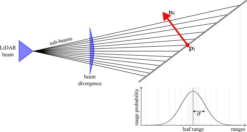
Figure 2: LiDAR uncertainty model. In the top image, a single LiDAR beam is simulated by casting a set of sub-beams towards a leaf $l$. At the bottom, the uncertainty of this measurement is modeled as a Gaussian distribution computed from the sampled ranges.

III-D Optimization

We perform BA to optimize both surfels and poses jointly. To carry on the minimization of Eq. (1), we employ the second-order LM method. Our optimization scheme performs a number of iterations up to a maximum or until convergence. We jointly optimize both surfels and poses within each iteration by leveraging an efficient Least Squares factor graph solver [11]. Each step is detailed in Alg. 2. While all 6-dof of poses are updated, surfels are constrained to move just along their normal direction. This approach preserves local geometry, simplifies optimization by reducing degrees of freedom, and aligns with LiDAR measurement uncertainty, which is greatest along the surfel normal. It also mitigates ambiguities in data association and ensures stable, physically meaningful refinements.

III-D1 Surfel creation

Surfels are created before optimization and maintained at each iteration. This ensures high-quality data association even if the initial set of poses is not so close to the optimum. It consists of two steps: finding associations between nearest-neighbor leaves by matching each kd-tree against every other and creating/updating surfels based on these associations. The idea is to group similar leaves observed from different poses. Surfels are generated by averaging the surfel centers $\mathbf{p}_{s}$ with the means of their corresponding leaf points $\mathbf{p}_{l}$, and by averaging the surfel normals $\mathbf{n}_{s}$ with the normals of the leaf points $\mathbf{n}_{l}$. The radius $r_{s}$ is set as the largest radius among the corresponding leaves to ensure it fully covers the variability of the points. Considering the sparsity of a LiDAR, this guarantees that the surfel adequately represents the local geometry, avoiding gaps or insufficient coverage that could lead to inconsistencies in the mapping process.

III-D2 Surfel normal updates

Measurement normals are a byproduct of the kd-tree creation, which occurs through PCA [8], only once at the beginning of BA. The construction is a recursive procedure that involves computing mean $\boldsymbol{\mu}$ and covariance $\mathbf{\Lambda}$ of the cloud $\mathcal{C}$. Then the eigenvectors $\mathbf{W}=\begin{bmatrix}\mathbf{w}_{0}&\mathbf{w}_{1}&\mathbf{w}_{2}\end{bmatrix}$ of $\mathbf{\Lambda}$ are sorted by eigenvalue. $\mathbf{w}_{2}$ is the direction of maximum variation, while $\mathbf{w}_{0}$ is the node’s normal. For terminal nodes, the latter vector corresponds to the observed surface normal. Surfel normal update is disconnected from non-linear BA optimization. Indeed, after each iteration, the tree leaves are re-grouped to update the surfel normal.

III-D3 Surfel position optimization

After updating normals $\mathbf{n}_{s}$ through kd-tree data matching, we jointly optimize poses and surfels using LM. Restricting surfel movement to their normal directions $q$ allows us to parameterize the updated surfel position as $q\mathbf{n}_{s}+\mathbf{p}_{s}$. This joint optimization of poses and surfels imposes fewer constraints, reducing discontinuities when refining different entities. Although independent surfel optimization is faster and parallelizable [19], the joint approach delivers superior results by effectively capturing the mutual dependencies between poses and structure, resulting in more consistent and accurate refinements.

III-D4 Pose optimization

Pose updates $\delta$ are parametrized as local updates in the Lie algebra $\mathfrak{se}(3)$. Thus, the transformation $\mathbf{T}_{k}^{w}$ of the local reference frame expressed in the global reference frame is updated as $\mathbf{T}_{k}^{w}\mathrm{exp}(\delta).$ Local updates ensure that rotation updates are well-defined [7]. This procedure is carried out for all the poses in the factor graph.

Algorithm 2 MAD-BA

input: clouds $\left\{\mathcal{C}\right\}$, initial poses $\left\{\mathbf{T}\right\}$
output: surfel set $\mathcal{S}^{*}$, refined poses $\left\{\mathbf{T}\right\}^{*}$

$\left\{\mathcal{T}\right\}$ $\leftarrow$ buildKdTrees($\left\{\mathcal{C}\right\}$) $\triangleright$ construct kd-trees

for $i\in$ # iterations do

  $\left\{\mathcal{T}\right\}$ $\leftarrow$ transform($\left\{\mathcal{T}\right\},\left\{\mathbf{T}\right\}$) $\triangleright$ transform kd-trees

  $\mathcal{S}\leftarrow$ createMatches($\left\{\mathcal{T}\right\}$) $\triangleright$ Alg. 1

  $\mathcal{S}^{*},\{\mathbf{T}\}^{*}\leftarrow$ optimize($\mathcal{S},\{\mathbf{T}\}$) $\triangleright$ optimize poses and surfels

IV Experimental Evaluation

		Initial trajectory		BALM2 [16]		HBA [15]		Pose-only		MAD-BA w/o uncert.		MAD-BA with uncert.
	Sequence	${\rm RMS}\downarrow$	${\rm MAX}\downarrow$	${\rm RMS}\downarrow$	${\rm MAX}\downarrow$	${\rm RMS}\downarrow$	${\rm MAX}\downarrow$	${\rm RMS}\downarrow$	${\rm MAX}\downarrow$	${\rm RMS}\downarrow$	${\rm MAX}\downarrow$	${\rm RMS}\downarrow$	${\rm MAX}\downarrow$
NC [18]	quad-easy	0.098	0.218	0.093	0.249	0.131	0.801	0.086	0.214	0.086	0.183	0.083	0.177
	maths-easy	0.090	0.189	0.162	0.420	0.135	0.606	0.087	0.189	0.054	0.163	0.043	0.176
	cloister	0.119	0.297	0.319	1.823	0.466	2.745	0.098	0.364	0.112	0.356	0.106	0.318
	stairs	0.368	0.717	0.366	0.700	3.104	9.088	0.375	1.429	0.067	0.126	0.070	0.132
	underground-easy	0.127	0.358	0.120	0.342	0.434	1.019	0.080	0.352	0.073	0.330	0.072	0.331
VBR [3]	Colosseo	2.920	5.873	2.877	5.553	1.123	2.763	2.891	5.887	0.698	1.585	0.565	1.161
	Spagna	0.963	1.912	1.058	5.479	1.628	4.625	1.053	3.953	0.412	1.229	0.155	0.522
	DIAG	0.341	0.804	0.425	1.945	0.960	2.510	0.335	2.014	0.101	0.438	0.103	0.455
	Campus	1.777	4.928	2.121	6.587	1.055	3.944	1.741	5.214	1.025	2.972	1.109	2.973
	Ciampino	6.078	16.097	6.086	15.669	5.641	16.645	6.040	15.881	3.878	13.711	3.123	9.566
	Pincio	1.488	2.914	1.719	3.293	1.508	4.589	1.499	3.304	0.914	3.177	1.121	3.869
KITTI [9]	00	5.232	11.291	5.585	16.075	4.899	9.897	5.145	11.326	3.717	7.657	3.544	6.473
	03	1.005	1.873	1.144	2.522	4.166	11.279	1.176	2.817	1.002	1.609	0.983	1.669
	04	0.444	1.162	0.507	1.226	0.532	1.776	0.399	1.075	0.411	1.111	0.521	1.371
	05	3.037	10.220	3.001	9.624	1.321	6.083	3.006	10.290	1.335	2.497	1.426	2.682
	06	1.400	2.039	2.498	19.379	0.668	1.488	1.350	2.179	0.856	1.747	0.892	1.819
	07	0.767	1.192	0.748	1.197	0.289	0.602	0.576	0.791	0.392	0.765	0.395	0.704
	08	4.034	12.668	8.198	67.587	4.553	12.815	4.027	12.319	6.535	16.982	5.449	14.873
	09	2.505	7.304	8.858	57.515	3.410	6.084	2.487	7.096	1.343	2.778	1.424	2.886
	10	2.024	3.720	2.725	10.738	4.179	8.107	2.051	3.807	1.854	4.193	2.191	4.422
	avg	1.741	4.289	2.430	11.396	2.010	5.373	1.725	4.525	1.243	3.181	1.169	2.829

TABLE I: Quantitative results of ATE for all tested methods across different publicly available datasets. Each error is reported in $\mathrm{m}$, and the last row of the table shows the total average of the error in each column. The best results for each sequence (the lowest ${\rm RMSE}$) are shown in bold.

In this section, we report the results of our method on different publicly available datasets. To quantitatively demonstrate the validity of our approach, we employ Absolute Trajectory Error (ATE) for pose estimation evaluation and the Chamfer-L1 distance to calculate the reconstruction accuracy. To run the experiments, we used a PC with an Intel Core i9-9900KF CPU @ 3.60GHz and 64GB of RAM. Our approach consists of a LiDAR BA to refine poses and scene geometry starting from an initialized set of poses and point clouds (i.e. LiDAR Odometry or SLAM), accompanied by a minimal set of parameters. The results show that our LiDAR BA strategy performs overall better than other existing approaches. Experimental evaluation supports our claim in a wide range of heterogeneous environments, including highways, narrow buildings, stairs, static and dynamic settings.

We report an extensive experimental campaign on the following datasets: Newer College Dataset (NC) [18], A Vision Benchmark in Rome (VBR) [3] and KITTI [9]. This experimental evaluation includes the comparison with LiDAR global refinement strategies: BALM2 [16] and HBA [15].

IV-A Datasets

For the evaluation, we used three publicly available datasets:

• NC [18]: Collected with a handheld Ouster OS0-128 LiDAR in structured and vegetated areas. Ground truth was generated using the Leica BLK360 scanner, achieving centimeter-level accuracy over poses and points in the map.

• VBR [3]: Recorded in Rome using OS1-64 (handheld) and OS0-128 (car-mounted) LiDARs, capturing large scale urban scenarios with narrow streets and dynamic objects. Ground truth trajectories were obtained by fusing LiDAR, IMU, and RTK GNSS data, ensuring centimeter-level accuracy over the poses.

• KITTI [9]: Recorded with a Velodyne HDL-64 in suburban and rural areas of Karlsruhe. While widely used in robotics and computer vision, its GPS/IMU-based ground truth is less accurate than modern high-precision systems, affecting error evaluation in certain sequences.

IV-B Evaluation method

Since this work focuses on achieving global consistency in both structure and poses, we perform quantitative evaluations using RMS of the ATE for the $\mathbb{SE}(3)$ poses and accuracy, completion, Chamfer-L1 distance, and F-score for the map. The first three parameters used for the map evaluation quantify the geometric discrepancy by measuring the average closest-point distance between the reconstructed map and a reference model, while the F-score measures how accurately they align to each other. For the poses, alignment is first achieved using the Horn method [12], with timestamps employed to establish pose associations. The RMSE is computed based on the translational differences between all matched poses. We use the three datasets for trajectory evaluation and restrict map evaluation to NC dataset, as it is the only one providing a high-resolution ground truth map. Specifically, given the reconstructed map $\mathcal{P}$ and a reference model $\mathcal{Q}$, the accuracy, completion and Chamfer-L1 distance are calculated as follows:

$$\small{d_{\text{C-L1}}(\mathcal{P},\mathcal{Q})=\underbrace{\frac{1}{2n}\sum_{p\in\mathcal{P}}\min_{q\in\mathcal{Q}}\|p-q\|}_{\text{accuracy}}+\underbrace{\frac{1}{2m}\sum_{q\in\mathcal{Q}}\min_{p\in\mathcal{P}}\|q-p\|}_{\text{completion}}}$$ (4)

where $m$ and $n$ are the number of points in $\mathcal{P}$ and $\mathcal{Q}$, respectively.

IV-C Parameters

All the compared systems require specifying certain parameters that impact their performance. For our method, the most important ones are those responsible for finding correspondences between surfels in the data association step:

• $d_{e}=0.5\,\mathrm{m}$: the maximum distance between the points of a surfel and a leaf that are considered for matching;

• $d_{n}=1.0\,\mathrm{m}$: the maximum distance between the points of a surfel and a leaf, calculated along the surfel’s normal;

• $d_{\theta}=5$°: the maximum angle between the normals of a surfel and a leaf;

• $\rho_{\mathrm{ker}}=0.1\,\mathrm{m}$: the threshold value for the Huber robust estimator during the factor graph optimization;

and for building the kd-trees:

• $b_{\mathrm{max}}=0.2\,\mathrm{m}$: the maximum size of kd-tree leaves;

• $b_{\mathrm{min}}=0.1\,\mathrm{m}$: the leaf’s minimum flatness below which its normal is propagated and assigned to its children.

It is important to note that these default values of the parameters were used during the evaluation, as they provide a consistent result across different sequences and datasets. In the case of HBA [15], we used the default parameter values, while for BALM2 [16], we changed the initial voxel size from $2\,\mathrm{m}$ to $1\,\mathrm{m}$, as it produced better results.

IV-D Comparison with State-of-the-art

We select two different approaches to compare our method. The first is BALM2 [16], a global LiDAR refinement approach that minimizes the distance from feature points to matched edges or planes. Unlike visual SLAM, where features are co-optimized with poses, BALM2 analytically eliminates features from the optimization, reducing computational complexity. However, this approach solely refines poses and does not optimize scene geometry, which limits its ability to handle structural inconsistencies in the map. Its reliance on an adaptive voxelization method for feature correspondence also restricts scalability in highly dynamic or complex environments.

The second approach is HBA [15], designed to address the computational challenges of LiDAR BA on large-scale maps. HBA employs a hierarchical framework that combines bottom-up BA with top-down pose graph optimization. While this design improves efficiency by reducing the optimization scale, the reliance on pose graph optimization decouples trajectory estimation from structure refinement, which can lead to inconsistencies in the final map, particularly for long trajectories or complex environments.

In contrast, our method integrates pose and structure optimization within a unified BA framework, eliminating the decoupling present in both BALM2 and HBA.

Table I summarizes the quantitative results for trajectory evaluation across all described methods and datasets. The first column shows the error for the initial trajectory, which is required as the starting point for all evaluated systems. We selected the open-source implementation of LOAM [29] for this purpose, as it remains one of the most widely used LiDAR-only odometry and mapping frameworks. However, for KITTI sequences 01 and 02, LOAM failed to produce estimates, so results for these sequences are omitted.

It is important to highlight that the quality of the initial trajectory significantly influences the performance of refinement systems. A poor initial guess can lead to incorrect scan correspondences, causing the optimization to converge to a local minimum. This limitation is evident in the results for BALM2 [16], presented in the second column. BALM2 often shows errors comparable to or worse than those of the initial trajectory, indicating that its voxel-based discretization struggles with the suboptimal starting poses provided by LOAM.

HBA [15], whose results are presented in the third column, performs better on certain sequences such as KITTI 05, 06, and 07, delivering the lowest errors. However, its performance is inconsistent across other datasets, further underscoring its sensitivity to the initial guess. In addition to multi-view ICP, this approach relies on PGO to simplify the optimization. While usually faster, is less accurate compared to BA. While parameter tuning could potentially improve the results of both BALM2 and HBA, we maintained a consistent configuration across all sequences to ensure a fair and unbiased evaluation, highlighting the general robustness of each system.

The last three columns in Tab. I present results for different variants of our system. The first variant evaluates our system configured to optimize only the poses while keeping all surfels fixed. The structure of the factor graph remains unchanged, but no adjustments are made to the surfels during optimization.

The next two columns show results for our BA method, demonstrating the impact of incorporating uncertainty into the optimization. In the first case, in Eq. (2), the uncertainty $\sigma=1$ assigns equal weight to all measurements. In the second case, $\sigma$ reflects the uncertainty estimated for each measurement during kd-tree creation, as detailed in Sec. III-C1. This strategy gives greater weight to measurement with higher confidence, improving both pose accuracy and map consistency. As expected, both BA configurations significantly reduce errors compared to keeping surfels fixed. Furthermore, incorporating uncertainty into the optimization enhances the overall results by leveraging confidence-weighted measurements.

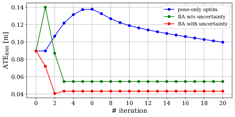
Figure 3: ATE for each iteration of the bundle adjustment algorithm. The plot compares three versions of our system for math-easy sequence and shows that both versions of our BA reduce the trajectory error and accelerate the converge of the algorithm related to the pose-only optimization. For BA with uncertainty, the error didn’t increase in the first iteration because measurements with higher uncertainty are weighted less during optimization.

Interestingly, Fig. 3 shows that considering uncertainty also reduces the number of iterations necessary to achieve convergence, especially compared to pose-only optimization.

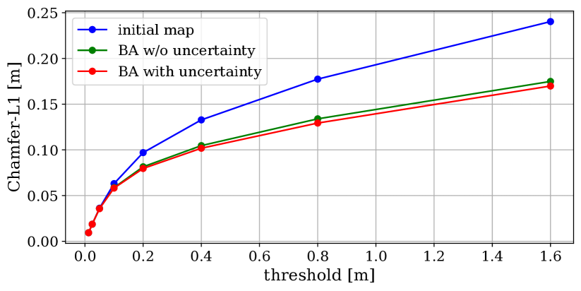
Figure 4: Chamfer-L1 distance of the cloister sequence for different distance thresholds. The initial map is a surfel map that was created using the initial trajectory. Both variants of our BA notably enhance the quality of the map, however, integrating uncertainty information results in additional improvements.

The map evaluation was performed by comparing the ground truth map with the surfel maps generated using the initial trajectory and those generated by MAD-BA with and without uncertainty information, as presented in Tab. II. The table also includes results for the point-based map from the HBA system for comparison. In order to exclude the non-overlapping parts of the refined and reference maps, we specified the threshold for the largest acceptable distance between points in these maps [5]. The threshold was set to $1\,\mathrm{m}$, however, as presented in Fig. 4, different values provide analogous results. Furthermore, we generated a comparison of the maps obtained from Newer College maths-easy and quad-easy sequences, presented in Fig. 5, which demonstrate a significant improvement in map quality after our bundle adjustment method. Another notable advantage of our map representation is that it implicitly disregards points that were registered on dynamic objects, such as driving cars or walking people. Although these filtering properties are hard to quantify, we present qualitative results of such a case for the part of VBR Spagna sequence in Fig. 6.

	initial map				HBA				MAD-BA w/o uncertainty				MAD-BA with uncertainty
Sequence	acc.$\downarrow$	comp.$\downarrow$	C-L1$\downarrow$	F-sc.$\uparrow$	acc.$\downarrow$	comp.$\downarrow$	C-L1$\downarrow$	F-sc.$\uparrow$	acc.$\downarrow$	comp.$\downarrow$	C-L1$\downarrow$	F-sc.$\uparrow$	acc.$\downarrow$	comp.$\downarrow$	C-L1$\downarrow$	F-sc.$\uparrow$
quad_easy	16.39	22.52	19.45	68.35	14.59	42.93	28.76	41.41	12.72	6.97	9.85	92.04	12.70	6.93	9.82	92.07
math_easy	19.22	26.87	23.05	58.55	16.86	43.49	30.17	38.70	14.44	10.65	12.55	87.20	14.35	10.54	12.44	87.26
cloister	22.78	16.31	19.54	69.18	18.62	39.18	28.90	45.76	21.78	7.34	14.56	77.86	21.18	6.95	14.06	78.96
stairs	28.91	23.66	26.29	55.51	33.82	32.35	33.08	41.41	24.32	7.22	15.77	73.50	24.56	7.28	15.92	73.36

TABLE II: Quantitative results of the map evaluation. The comparison includes the following metrics: accuracy (acc.), completion (comp.), Chamfer-L1 (C-L1), and F-score (F-sc.). The first three metrics are given in centimeters, while the F-score is expressed as a percentage. The column initial map presents results for surfel map created using the initial trajectory before applying our LiDAR Bundle Adjustment method. A threshold of $1\,\mathrm{m}$ was used to exclude non-overlapping regions of the map, and an additional threshold of $0.2\,\mathrm{m}$ was used to calculate F-score. Overall, incorporating uncertainty improves performance, except in the stairs sequence, which features narrow corridors where individual measurements are already highly reliable. The underground-easy is not included in this table, as there is no ground truth map for this sequence.

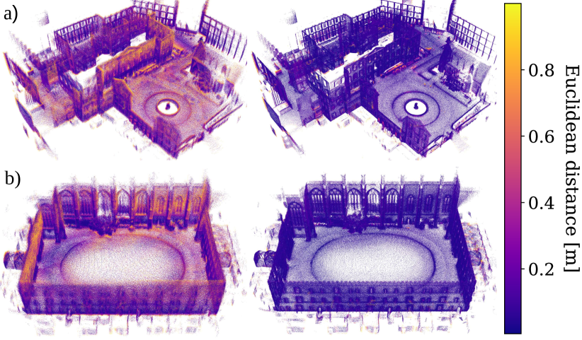
Figure 5: Qualitative results of the maps generated from NC math-easy (a) and NC quad-easy (b) sequences, where the color of each surfel’s point corresponds to its Euclidean distance to the nearest point in the ground truth map. The left-side images are created before the optimization (using the initial trajectory), while the right ones after our BA with uncertainty method.

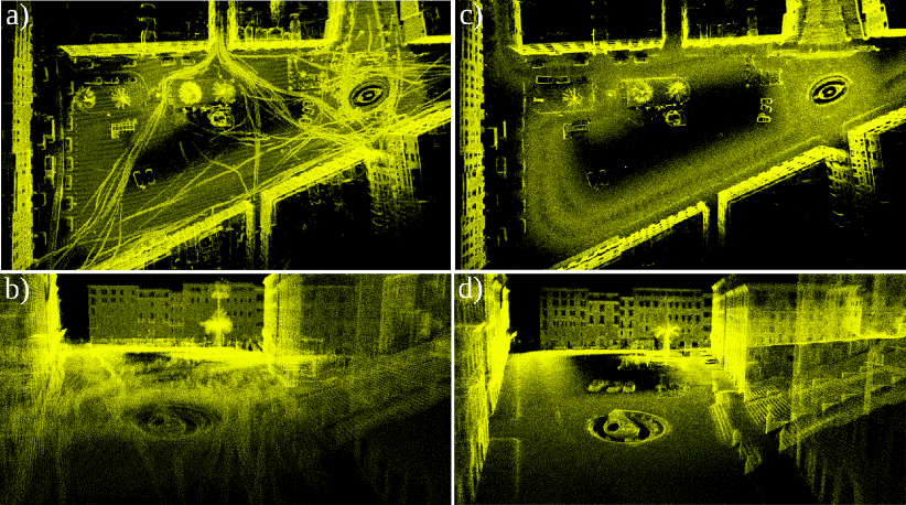
Figure 6: Qualitative map results. Map insets generated for VBR Spagna sequence by LOAM (a,b) and our MAD-BA method showing the surfel map converted to point cloud (c,d). A benefit of our approach is that it produces a crisp representation of the environment, compensating for noise and filtering points from moving objects, such as cars and people in motion.

V Conclusion

This work presents a novel framework for the simultaneous optimization of poses and 3D map, with the map represented using a 3D surfel-based parameterization. Additionally, we introduce a generalized LiDAR uncertainty model, enabling accurate weighting during the optimization process. Our experimental results across multiple public datasets demonstrate that the proposed system outperforms existing LiDAR-based pose and map estimation methods in terms of robustness and accuracy. The framework achieves precise estimation of poses and map and inherently mitigates dynamic artifacts and LiDAR skewing effects, resulting in consistent and clean maps—a critical aspect for applications requiring high-fidelity 3D representations. The open-source implementation of our system aims to benefit the community. Future work will explore enhancing scalability for even larger environments, integrating multi-modal sensor data such as cameras and inertial sensors, and extending the framework to handle highly dynamic environments explicitly. Additionally, we aim to investigate real-time implementations to bridge the gap between batch optimization and practical deployment in robotics and autonomous systems.

References

- [1] Emmanuel P Baltsavias. Airborne laser scanning: basic relations and formulas. ISPRS Journal of Photogrammetry and Remote Sensing (JPRS), 54(2-3):199–214, 1999.
- [2] Jens Behley and Cyrill Stachniss. Efficient surfel-based SLAM using 3d laser range data in urban environments. In Hadas Kress-Gazit, Siddhartha S. Srinivasa, Tom Howard, and Nikolay Atanasov, editors, Robotics: Science and Systems XIV, Carnegie Mellon University, Pittsburgh, Pennsylvania, USA, June 26-30, 2018, 2018.
- [3] Leonardo Brizi, Emanuele Giacomini, Luca Di Giammarino, Simone Ferrari, Omar Salem, Lorenzo De Rebotti, and Giorgio Grisetti. VBR: A vision benchmark in Rome. In Proc. of the IEEE Intl. Conf. on Robotics & Automation (ICRA), pages 15868–15874, 2024.
- [4] Krzysztof Ćwian, Michał R. Nowicki, Jan Wietrzykowski, and Piotr Skrzypczyński. Large-scale LiDAR SLAM with factor graph optimization on high-level geometric features. Sensors, 21(10), 2021.
- [5] Junyuan Deng, Qi Wu, Xieyuanli Chen, Songpengcheng Xia, Zhen Sun, Guoqing Liu, Wenxian Yu, and Ling Pei. NeRF-LOAM: Neural implicit representation for large-scale incremental lidar odometry and mapping. In IEEE/CVF International Conference on Computer Vision (ICCV), pages 8184–8193, 2023.
- [6] Luca Di Giammarino, Emanuele Giacomini, Leonardo Brizi, Omar Salem, and Giorgio Grisetti. Photometric LiDAR and RGB-D bundle adjustment. IEEE Robotics and Automation Letters (RA-L), 2023.
- [7] Chris Engels, Henrik Stewénius, and David Nistér. Bundle adjustment rules. Photogrammetric computer vision, 2(32), 2006.
- [8] Simone Ferrari, Luca Di Giammarino, Leonardo Brizi, and Giorgio Grisetti. MAD-ICP: It is all about matching data – robust and informed LiDAR odometry. IEEE Robotics and Automation Letters (RA-L), 9(11):9175–9182, 2024.
- [9] A. Geiger, P. Lenz, C. Stiller, and R. Urtasun. Vision meets robotics: The KITTI dataset. Intl. Journal of Robotics Research (IJRR), 32(11):1231–1237, 2013.
- [10] L. Di Giammarino, L. Brizi, T. Guadagnino, C. Stachniss, and G. Grisetti. Md-slam: Multi-cue direct SLAM. In Proc. of the IEEE/RSJ Intl. Conf. on Intelligent Robots and Systems (IROS), pages 11047–11054. IEEE, 2022.
- [11] G. Grisetti, T. Guadagnino, I. Aloise, M. Colosi, B. Della Corte, and D. Schlegel. Least squares optimization: From theory to practice. Robotics, 9(3):51, 2020.
- [12] B. Horn, H. Hilden, and S. Negahdaripour. Closed-form solution of absolute orientation using orthonormal matrices. JOSA A, 5(7):1127–1135, 1988.
- [13] Yihua Hu, Ahui Hou, Qingli Ma, Nanxiang Zhao, Shilong Xu, and Jiajie Fang. Analytical formula to investigate the modulation of sloped targets using LiDAR waveform. Transactions on Geoscience and Remote Sensing, 60:1–12, 2021.
- [14] Shengyu Huang, Zan Gojcic, Zian Wang, Francis Williams, Yoni Kasten, Sanja Fidler, Konrad Schindler, and Or Litany. Neural LiDAR fields for novel view synthesis. In Proc. of the IEEE Intl. Conf. on Computer Vision (ICCV), pages 18236–18246, 2023.
- [15] Xiyuan Liu, Zheng Liu, Fanze Kong, and Fu Zhang. Large-scale LiDAR consistent mapping using hierarchical lidar bundle adjustment. IEEE Robotics and Automation Letters (RA-L), 8(3):1523–1530, 2023.
- [16] Z. Liu and F. Zhang. Balm: Bundle adjustment for LiDAR mapping. IEEE Robotics and Automation Letters (RA-L), 6(2):3184–3191, 2021.
- [17] James McNames. A fast nearest-neighbor algorithm based on a principal axis search tree. IEEE Trans. on Pattern Analalysis and Machine Intelligence (TPAMI), 23(9):964–976, 2001.
- [18] M. Ramezani, Y. Wang, M. Camurri, D. Wisth, M. Mattamala, and M. Fallon. The Newer College dataset: Handheld LiDAR, inertial and vision with ground truth. In Proc. of the IEEE/RSJ Intl. Conf. on Intelligent Robots and Systems (IROS), pages 4353–4360, 2020.
- [19] T. Schops, T. Sattler, and M. Pollefeys. Bad SLAM: Bundle adjusted direct RGBD-D SLAM. In Proc. of the IEEE Conf. on Computer Vision and Pattern Recognition (CVPR), pages 134–144, 2019.
- [20] Piotr Skrzypczynski. Spatial uncertainty management for simultaneous localization and mapping. In Proceedings 2007 IEEE International Conference on Robotics and Automation, pages 4050–4055, 2007.
- [21] T. Stoyanov, M. Magnusson, H. Andreasson, and A. J. Lilienthal. Fast and accurate scan registration through minimization of the distance between compact 3D NDT representations. Intl. Journal of Robotics Research (IJRR), 31(12):1377–1393, 2012.
- [22] Bill Triggs, Philip F. McLauchlan, Richard I. Hartley, and Andrew W. Fitzgibbon. Bundle adjustment — a modern synthesis. In Bill Triggs, Andrew Zisserman, and Richard Szeliski, editors, Vision Algorithms: Theory and Practice, pages 298–372, Berlin, Heidelberg, 2000. Springer Berlin Heidelberg.
- [23] M. Velas, M. Spanel, and A. Herout. Collar line segments for fast odometry estimation from Velodyne point clouds. In Proc. of the IEEE Intl. Conf. on Robotics & Automation (ICRA), pages 4486–4495, 2016.
- [24] I. Vizzo, T. Guadagnino, B. Mersch, L. Wiesmann, J. Behley, and C. Stachniss. Kiss-ICP: In defense of point-to-point ICP – simple, accurate, and robust registration if done the right way. IEEE Robotics and Automation Letters (RA-L), 8(2):1029–1036, 2023.
- [25] Aloysius Wehr and Uwe Lohr. Airborne laser scanning—an introduction and overview. ISPRS Journal of Photogrammetry and Remote Sensing (JPRS), 54(2-3):68–82, 1999.
- [26] Lan Wu, Cedric Le Gentil, and Teresa Vidal-Calleja. VDB-GPDF: Online Gaussian process distance field with VDB structure. IEEE Robotics and Automation Letters (RA-L), 10(1):374–381, 2025.
- [27] Fan Xu, Yuanqing Wang, Xingyu Yang, Bingqing Zhang, and Fenfang Li. Correction of linear-array lidar intensity data using an optimal beam shaping approach. Optics and Lasers in Engineering, 83:90–98, 2016.
- [28] J. Zhang, M. Kaess, and S. Singh. On degeneracy of optimization-based state estimation problems. In Proc. of the IEEE Intl. Conf. on Robotics & Automation (ICRA), pages 809–816, 2016.
- [29] J. Zhang and S. Singh. LOAM: Lidar odometry and mapping in real-time. In Proc. of Robotics: Science and Systems (RSS), 2014.