Impact of Leg Stiffness on Energy Efficiency in One Legged Hopping

Abstract

In the fields of robotics and biomechanics, the integration of elastic elements such as springs and tendons in legged systems has long been recognized for enabling energy-efficient locomotion. Yet, a significant challenge persists: designing a robotic leg that perform consistently across diverse operating conditions, especially varying average forward speeds. It remains unclear whether, for such a range of operating conditions, the stiffness of the elastic elements needs to be varied or if a similar performance can be obtained by changing the motion and actuation while keeping the stiffness fixed. This work explores the influence of the leg stiffness on the energy efficiency of a monopedal robot through an extensive parametric study of its periodic hopping motion. To this end, we formulate an optimal control problem parameterized by average forward speed and leg stiffness, solving it numerically using direct collocation. Our findings indicate that, compared to the use of a fixed stiffness, employing variable stiffness in legged systems improves energy efficiency by $20\,\%$ maximally and by $6.8\,\%$ on average across a range of speeds.

Index Terms—Design Optimization, Optimal Actuation, Periodic Orbits, Legged Systems

I INTRODUCTION

Legged robots are useful in many fields, including industrial inspection, search and rescue or exploration [1, 2, 3]. However, their full potential cannot be exploited yet, due to multiple factors. Especially reliability and energy economic aspects are considered major challenges to the real-world adoption of legged robots [4, 5].

A multitude of factors influence the energy economy of legged robotic systems. For example, gait patterns [6], actuator [7] and leg design [8] have all been reported to have an influence. Yet, one of the most important ingredients to design an energy efficient legged robot is the introduction of passive dynamics through leg compliance [9]. A spring-like leg behavior is essential to be able to access a variety of different gaits [10, 11], which in turn have a large influence on the efficiency of legged systems [12]. Additionally, gait selection is greatly dependent on the speed a system moves at [10, 12]. Thus, the dynamics are to a great extent shaped by the interplay between leg compliance and speed. Therefore, it is of much interest to study its influence on the energy economics of legged robots.

Elastic leg behavior is present in a large range of animals, including birds, mammals, insects and other arthropods [13]. In the case of the human leg, elasticity originates primarily from the muscles and tendons of the knee and ankle joints [14]. Humans commonly adapt their leg stiffness depending on certain factors, for example slope [15], ground compliance [16, 17] or stride frequency [14]. Despite that, no correlation between stiffness and speed has been observed, except for fast running, which might be due to methodology [18, 19]. For instance, [14] shows that human running is equally efficient with a variety of leg stiffness values over different speeds.

It has been shown that simple models allow for investigation of underlying principles in legged locomotion [20], including the study of leg compliance [21, 22]. A common practice in research is to model running motions with the Spring-Loaded Inverted Pendulum (SLIP) [23] developed by Blickhan [24]. The SLIP, as well as its extensions [25, 26, 27, 28, 29, 30, 22], allow for a definition of the so-called leg stiffness by modeling the leg as a spring.

Multiple studies on leg stiffness of legged robots have been conducted over the years. Tsagarakis et al. [31] have computed the stiffness by maximizing the energy stored in the spring during locomotion. Rummel et al. [32] have analyzed a bipedal SLIP-like model in terms of robustness and efficiency and proposed a lower bound to leg stiffness. Schroeder et al. [27] have computed energetically optimized gaits for the SLIP and two extended SLIP models, considering different leg stiffness values. They came to the conclusion that smaller stiffness values are always more efficient. Yet, there still exists no universal approach to calculating an optimal stiffness value for a certain problem configuration.

Much research has also been committed to studying the effects of speed on energy economics of legged robots. Ahmadi et al. [33] built a single-legged hopper and found that its energy consumption increased quadratically with speed. Xi et al. [12] have found energetically optimal speeds for walking and running of biped and quadruped models.

Apart form the search for individual optimal parameters, much research has been conducted in the field of variable stiffness mechanisms for legged robots. Based on the idea that leg stiffness has a significant influence on the energy consumption over various conditions, some research have proposed using variable stiffness mechanisms for legged robots. It has been shown that certain robots improve their energy economics by applying terrain-dependent learned stiffness patterns [34, 35]. Vu et al. [29] have looked at the interplay between stride frequency, energy economics and leg stiffness through simulation and experiments and came to the conclusion that variable stiffness mechanisms improve the efficiency of legged robots. The research of Galloway et al. [36, 37] produced similar results for stiffness adaption based on speed. However, the question has been raised, if such mechanisms are worthwhile due to the added weight and complexity [38].

In this study, we investigate the interplay between leg stiffness, average velocity, and energetic economy, using a two-dimensional monopedal robot. The monoped serves as a more sophisticated template for running compared to the commonly used SLIP model [24]. Unlike the SLIP model, our model incorporates both inertia and foot mass, providing a more detailed representation of running dynamics. The simplicity of the monopedal model, combined with its resemblance to running motion, makes it an ideal framework for exploring fundamental principles of energy-efficient locomotion. We conduct an extensive parametric search over varying leg stiffness values and forward speeds, formulating an optimization problem to identify optimal gaits.

Studying the influence of parameters on the economy of legged robots requires the use of optimization algorithms to identify the most economic gaits under specific conditions. Due to the complexity of the hybrid dynamics of legged systems and the vastness of the search space, solving these algorithms is far from trivial [39]. When exploring a broad range of optimal gaits, continuation methods provide a straightforward approach to generating families of neighboring gaits. Key contributions to continuation methods in legged locomotion are presented in [20, 40, 41]. In this work, we use a closely related but simpler method to generate a three-dimensional surface that maps average speed and leg stiffness to the cost of these optimal motions.

In the remainder of this paper, we first introduce the dynamics of the monopedal robot and formulate the optimal control problem used in the study (Section II), before discussing the numerical algorithms used to generate the mapping of optimal gaits (Section III). We discuss the results in Section IV and formulate our conclusions in Section V.

II PROBLEM FORMULATION

This section introduces the model and hybrid dynamics of a monoped hopper equipped with parallel-elastic actuators. We then formulate a parameterized optimization problem to minimize the robot’s cost of transport across varying leg stiffness values and average velocities.

II-A Dynamical Model of a Monopedal Robot

We consider the planar monopedal robot shown in Fig. 1, based on the model presented in [40]. The robot consists of a torso with mass $m_{\mathrm{t}}$ and inertia $\Theta_{\mathrm{t}}$, connected through a revolute hip joint to a single leg. The leg comprises an upper segment with mass $m_{\mathrm{l}}$, inertia $\Theta_{\mathrm{l}}$, and a center of mass (CoM) located a distance $d_{\mathrm{l}}$ from the hip. The upper segment connects through a prismatic joint to a lower segment with mass $m_{\mathrm{f}}$, inertia $\Theta_{\mathrm{f}}$, and a spherical foot (radius $r_{\mathrm{f}}$) whose CoM lies $d_{\mathrm{f}}$ above its center.

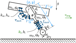
Figure 1: A monopedal robot with parallel elastic actuation in the leg and hip joint.

The torso’s position is defined by the hip coordinates $(x,y)$ and the pitch angle $\varphi$. The upper leg’s orientation is measured by the hip angle $\alpha$, while the overall leg length $l$ captures the prismatic joint’s extension. We define the generalized coordinates as $\bm{q}^{\mathop{\mathrm{T}}}=[x~y~\phi~\alpha~l]$, with $n_{q}=5$ degrees of freedom. For readability, time dependencies are omitted in the remainder of this work.

The robot is actuated by a torque $\tau_{\mathrm{mot}}$ at the hip and a translational force $f_{\mathrm{mot}}$ at the leg joint, forming the control input $\bm{u}^{\mathop{\mathrm{T}}}=[\tau_{\mathrm{mot}}~f_{\mathrm{mot}}]$. Both actuators are co-located with springs (stiffness value coefficients $k_{\alpha}$ and $k_{\mathrm{l}}$) and dampers (damping ratios $\xi_{\alpha}$ and $\xi_{\mathrm{l}}$), creating parallel elastic actuation. The model parameters are normalized using total body mass $m$, natural leg length $l_{\circ}$, and gravity $g$, following [42]. All parameters, but the leg stiffness $k_{\mathrm{l}}$ are fixed. Table I lists all the parameter values used in this study.

$m_{\mathrm{f}}$	$=~0.05~m$	$k_{\alpha}$	$=~5~mgl_{\circ}/\mathrm{rad}$
$m_{\mathrm{l}}$	$=~0.1~m$	$\xi_{\mathrm{l}}$	$=~0.2\sqrt{2}~m\sqrt{g/l_{\circ}}$
$m_{\mathrm{t}}$	$=~0.85~m$	$\xi_{\alpha}$	$=~0.2~m_{\mathrm{f}}gl_{o}/\mathrm{rad}$
$\Theta_{\mathrm{f}}$	$=~0.002~ml_{\circ}^{2}$	$r_{\mathrm{f}}$	$=~0.05~l_{\circ}$
$\Theta_{\mathrm{l}}$	$=~0.002~ml_{\circ}^{2}$	$d_{\mathrm{l}}$	$=~0.25~l_{\circ}$
$\Theta_{\mathrm{t}}$	$=~0.4~ml_{\circ}^{2}$	$d_{\mathrm{f}}$	$=~0.25~l_{\circ}$

TABLE I: Model parameters normalized by total body mass $m$, natural leg length $l_{\circ}$, and gravity $g$, adapted from [43].

The damping coefficients are expressed as

$$b_{\mathrm{l}} =2\xi_{\mathrm{l}}\sqrt{k_{l}(m_{\mathrm{t}}+m_{\mathrm{l}})},$$ (1a)

$$b_{\alpha} =2\xi_{\alpha}\sqrt{k_{\alpha}\left(\Theta_{\mathrm{l}}+m_{\mathrm{l}}d_{\mathrm{l}}^{2}+\Theta_{\mathrm{f}}+m_{\mathrm{f}}(l_{\circ}+d_{\mathrm{f}})^{2}\right)}.$$ (1b)

Having one leg, the monopedal robot can only hop to move forward. This provides a crucial simplification in the study, as the gait pattern can be a priori fixed in the optimization problem. A hopping gait consists of two phases: Stance (S) with a duration $t^{\mathrm{S}}$ and Flight (F) with a duration $t^{\mathrm{F}}$. The robot starts its stride at touch-down at the beginning of the stance phase, during which the foot remains in contact with the ground. During contact, the foot is constrained to pure rolling motion, resulting in the constraints $\bm{c}^{\mathop{\mathrm{T}}}=[c_{x}~c_{y}]$, where

$$c_{x}(\bm{q}) =x+r_{\text{f}}(\varphi+\alpha)+l\sin(\varphi+\alpha)-d_{0},$$ (2a)

$$c_{y}(\bm{q}) =y-l\cos{(\varphi+\alpha)}-r_{\text{f}},$$ (2b)

with $d_{0}=x_{0}+(\varphi_{0}+\alpha_{0})r_{\text{f}}+l_{0}\sin(\varphi_{0}+\alpha_{0})$ and $x_{0},\varphi_{0},\alpha_{0},l_{0}$ being the values of $x,\varphi,\alpha$ and $l$ at touchdown.

With the contact Jacobian $\bm{W}(\bm{q})=\nicefrac{{\partial\bm{c}}}{{\partial\bm{q}}}$ and contact forces $\bm{\lambda}^{\mathop{\mathrm{T}}}=[\lambda_{x}~\lambda_{y}]$, the stance dynamics are described by

$$\bm{M}(\bm{q})\ddot{\bm{q}}=\bm{h}(\bm{q},\dot{\bm{q}})+\bm{W}^{\mathop{\mathrm{T}}}(\bm{q})\bm{\lambda}+\bm{B}\bm{u},$$ (3)

where $\bm{M}$ is the mass matrix, $\bm{h}$ accounts for Coriolis and centrifugal forces and $\bm{B}$ is the input matrix.

To solve the differential algebraic equation (2), we perform an index reduction and differentiate the constraints twice (i.e., $\ddot{\bm{c}}=0$) to arrive at $\bm{W}(\bm{q})\ddot{\bm{q}}=-\dot{\bm{W}}(\bm{q})\dot{\bm{q}}$. With Eq. (3), $\bm{\lambda}$ becomes a function of $\bm{x}^{\mathop{\mathrm{T}}}=[\bm{q}^{\mathop{\mathrm{T}}}~\dot{\bm{q}}^{\mathop{\mathrm{T}}}]$ and $\bm{u}$. Hence, the stance dynamics (3) can be compactly written as

$$\dot{\bm{x}}=\bm{f}_{\mathrm{S}}(\bm{x},\bm{u};k_{\mathrm{l}}),$$ (4)

where the leg stiffness, $k_{\mathrm{l}}$, is explicitly included in the function parameters as a variable system parameter.

At liftoff, the normal contact force $\lambda_{y}(\bm{x},\bm{u};k_{\mathrm{l}}$) vanishes and the robot transitions to the flight phase. During flight, the contact forces are constant zero (i.e., $\bm{\lambda}=\bm{0}$). Hence, the flight dynamics (3) take the compact form

$$\dot{\bm{x}}=\bm{f}_{\mathrm{F}}(\bm{x},\bm{u};k_{\mathrm{l}}).$$ (5)

The stride ends when the foot returns to the ground, satisfying $c_{y}(\bm{x})=0$. This instance of touch-down results in a discontinuous change in $\dot{\bm{q}}$, which is represented by the jump map:

$$\bm{x}^{+}=\bm{g}(\bm{x}^{-}),$$ (6)

where $\bm{x}^{-}$ and $\bm{x}^{+}$ denote the states before and after the collision, respectively.

II-B Parameterized Trajectory Optimization

We formulate an optimization problem based on the robot’s dynamics to determine the optimal motion for the monoped. Since only periodic hopping motion are of interest, the optimization is performed over a single stride. In the following, we distinguish between stance and flight trajectories, denoting them as $\big{(}\bm{x}^{\mathrm{S}}(t),\bm{u}^{\mathrm{S}}(t)\big{)}$, with $t\in[0,t^{\mathrm{S}}]$, for stance and $\big{(}\bm{x}^{\mathrm{F}}(t),\bm{u}^{\mathrm{F}}(t)\big{)}$, with $t\in[0,t^{\mathrm{F}}]$, for flight. While the robot’s motion is initialized at the horizontal position $x^{\text{S}}(0)=0$, the remaining states must exhibit periodicity, meaning the post-impact values at the end of the stride must match the initial conditions such that $\bm{x}^{\mathrm{S}}(0)=\bm{S}\bm{g}\big{(}\bm{x}^{\mathrm{F}}(t^{\mathrm{F}})\big{)}$. The selection matrix $\bm{S}=\text{diag}(0,1,\ldots,1)\in\mathbb{R}^{10\times 10}$ accounts for the fact that the horizontal position is non-periodic and that instead the initial horizontal position should be set to zero. To further specify the robot’s periodic operating point, we constrain the average forward speed $v_{\text{avg}}$.

With parameters $k_{\mathrm{l}}$ and $v_{\mathrm{avg}}$, we define the parameterized trajectory optimization problem

$$\begin{array}[]{cl}\hline\cr\\[-5.69054pt] \mathcal{P}({\color[rgb]{0.09,0.51,0}k_{\mathrm{l}}},{\color[rgb]{0.09,0.51,0}v_{\mathrm{avg}}}):&\\ \displaystyle\mathop{\mathrm{minimize}}_{\begin{subarray}{c}\bm{x}^{\mathrm{S}}(\cdot),\bm{u}^{\mathrm{S}}(\cdot),t^{\mathrm{S}},\\ \bm{x}^{\mathrm{F}}(\cdot),\bm{u}^{\mathrm{F}}(\cdot),t^{\mathrm{F}}\end{subarray}}&\displaystyle\frac{1}{mg\Delta x}\left(\displaystyle\int\limits_{0}^{t^{\mathrm{S}}}\lVert\bm{u}^{\mathrm{S}}(t)\rVert_{\bm{K}}^{2}\mathrm{d}{t}+\displaystyle\int\limits_{0}^{t^{\mathrm{F}}}\lVert\bm{u}^{\mathrm{F}}(t)\rVert_{\bm{K}}^{2}\mathrm{d}{t}\right)\\[25.60747pt] \text{subject to}&\dot{\bm{x}}^{\mathrm{S}}(t)=\bm{f}_{\mathrm{S}}(\bm{x}^{\mathrm{S}}(t),\bm{u}^{\mathrm{S}}(t);{\color[rgb]{0.09,0.51,0}k_{\mathrm{l}}}),~~~\forall t\in[0,t^{\mathrm{S}}],\\[5.69054pt] &\dot{\bm{x}}^{\mathrm{F}}(t)=\bm{f}_{\mathrm{F}}(\bm{x}^{\mathrm{F}}(t),\bm{u}^{\mathrm{F}}(t);{\color[rgb]{0.09,0.51,0}k_{\mathrm{l}}}),~~\forall t\in[0,t^{\mathrm{F}}],\\[5.69054pt] &\lambda_{y}\big{(}\bm{x}^{\mathrm{S}}(t^{\mathrm{S}}),\bm{u}^{\mathrm{S}}(t^{\mathrm{S}});{\color[rgb]{0.09,0.51,0}k_{\mathrm{l}}}\big{)}=0,\\[5.69054pt] &\bm{x}^{\mathrm{F}}(0)=\bm{x}^{\mathrm{S}}(t^{\mathrm{S}}),\\[5.69054pt] &c_{y}\big{(}\bm{x}^{\mathrm{F}}(t^{\mathrm{F}})\big{)}=0,\\[5.69054pt] &\bm{x}^{\mathrm{S}}(0)=\bm{S}\bm{g}\big{(}\bm{x}^{\mathrm{F}}(t^{\mathrm{F}})\big{)},\\[5.69054pt] &\underbrace{{\color[rgb]{0.09,0.51,0}v_{\mathrm{avg}}}\cdot(t^{\mathrm{S}}+t^{\mathrm{F}})}_{=\Delta x}=x^{\mathrm{F}}(t^{\mathrm{F}}),\\[19.91692pt] \hline\cr\end{array}$$

where the cost of transport (CoT) objective corresponds to thermal losses of a DC-motor with speed-torque gradient matrix $\bm{K}=\mathrm{diag}\big{(}m\sqrt{gl_{\circ}^{3}},m\sqrt{g/l_{\circ}}\big{)}^{-1}$ normalized over distance traveled $\Delta x$.

III NUMERICAL IMPLEMENTATION

III-A Direct Collocation

To numerically solve the optimization problem $\mathcal{P}$, we use direct collocation with a Hermite–Simpson scheme for discretization, as outlined in [44]. Given the fixed foot-pattern in the hopping gait, the stance and flight phase dynamics are treated as two separate systems, connected through events, jump maps and periodicity constraints. The state trajectory is parametrized by a cubic spline, resulting in piecewise quadratic dynamics and cost functions. The time domains of stance and flight are divided into $N$ equidistant segments. Each one starts at $t_{0}=0$ and ends at $t_{N}=t^{\mathrm{S}}$ and $t_{N}=t^{\mathrm{F}}$ respectively.

Consider the dynamics of any phase, denoted by $\bm{f}$, with the state vector $\bm{x}$ and the input vector $\bm{u}$. For any time-dependent variable $\chi$, we define:

$$\chi_{k}:=\chi(t_{k})\qquad\text{and}\qquad\chi_{k+\frac{1}{2}}:=\chi\left(t_{k}+\frac{\Delta t}{2}\right),$$ (7)

where $\Delta t=\frac{t_{N}}{N}$.

Let $w$ denote the running cost, i.e.,

$$w(t)=\lVert\bm{u}(t)\rVert_{\bm{K}}^{2}.$$ (8)

Using Simpsons quadrature, the total cost during a phase is approximated as

$$\int\limits_{0}^{t_{N}}w(\tau)\,d\tau\approx\frac{\Delta t}{6}\sum_{k=0}^{N-1}(w_{k}+w_{k+\frac{1}{2}}+w_{k+1}).$$ (9)

At the midpoint of each segment, we enforce the dynamics through the collocation constraints:

$$\bm{x}_{k+\frac{1}{2}} =\frac{1}{2}(\bm{x}_{k}+\bm{x}_{k+1})+\frac{\Delta t}{8}(\dot{\bm{x}}_{k}+\dot{\bm{x}}_{k+1})$$ (10a)

$$\dot{\bm{x}}_{k+\frac{1}{2}} =\frac{-3}{2\Delta t}(\bm{x}_{k}-\bm{x}_{k+1})+\frac{1}{4}(\dot{\bm{x}}_{k}+\dot{\bm{x}}_{k+1}).$$ (10b)

We additionally assume that the input $\bm{u}$ is continuously differentiable. To enforce this, we introduce the input derivative:

$$\bm{v}:=\dot{\bm{u}}.$$ (11)

Let $\tilde{\bm{x}}=\begin{bmatrix}\bm{x}&\bm{u}\end{bmatrix}^{\mathop{\mathrm{T}}}$ be the extend state vector. Using Eq. (11), the dynamics are defined as,

$$\dot{\tilde{\bm{x}}}=\tilde{f}(\tilde{\bm{x}},\bm{v})=\begin{bmatrix}f(\bm{x},\bm{u})\\ \bm{v}\end{bmatrix}$$ (12)

To enforce piecewise linearity and continuity of the extended dynamics’ control input, we add the constraint

$$\bm{v}_{k+\frac{1}{2}}=\frac{1}{2}(\bm{v}_{k}+\bm{v}_{k+1}),$$ (13)

enforcing the integrand $\bm{u}$ to be continuously differentiable.

The parametrized optimization problem $\mathcal{P}$ is reformulated as a Nonlinear Program (NLP) by incorporating collocation constraints for the dynamics, summing the approximated total costs, and imposing event constraints at the end of each phase. The remaining constraints in $\mathcal{P}$ are directly transferred into the NLP formulation.

All states and controls at the grid points, along with the durations of the stance and flight phases, constitute the decision variables of the NLP. We define the vector of decision variables as:

$$\bm{a}_{\mathcal{N}}=\big{[}\tilde{\bm{x}}^{S}_{0}~\bm{v}^{S}_{0}~\ldots~\tilde{\bm{x}}^{S}_{N}~\bm{v}^{S}_{N}~t^{\mathrm{S}}~\tilde{\bm{x}}^{F}_{0}~\bm{v}^{F}_{0}~\ldots~\tilde{\bm{x}}^{F}_{N}~\bm{v}^{F}_{N}~t^{\mathrm{F}}\big{]}.$$ (14)

All the aforementioned constraints can be reformulated as a residual function,

$$\bm{h}(\bm{a}_{\mathcal{N}};k_{\mathrm{l}},v_{\mathrm{avg}})=0.$$ (15)

We further introduce inequality constraints of the form

$$\bm{g}(\bm{a}_{\mathcal{N}},k_{\mathrm{l}},v_{\mathrm{avg}})<\bm{b},$$ (16)

where $\bm{b}$ is a vector of bounds on certain elements of $\bm{a}$. These bounds, represent physical limitations that would be present in a real robot, to ensure that the solution space corresponds to realistic hopping gaits.

The resulting NLP is given by,

$$\begin{array}[]{cl}\hline\cr\\[-5.69054pt] \mathcal{N}({\color[rgb]{0.09,0.51,0}k_{\mathrm{l}}},{\color[rgb]{0.09,0.51,0}v_{\mathrm{avg}}}):&\\ \displaystyle\mathop{\mathrm{minimize}}_{\bm{a}_{\mathcal{N}}}&\displaystyle\frac{1}{mg\Delta x}\Bigg{(}\displaystyle\sum_{k=0}^{N}\frac{\Delta_{t}^{\text{S}}}{6}(w^{\text{S}}_{k}+4w^{\text{S}}_{k+\frac{1}{2}}+w^{\text{S}}_{k+1})\\ &+\displaystyle\sum_{k=0}^{N}\frac{\Delta_{t}^{\text{F}}}{6}(w^{\text{F}}_{k}+4w^{\text{F}}_{k+\frac{1}{2}}+w^{\text{F}}_{k+1})\Bigg{)}\\[19.91692pt] \text{subject to}&\bm{h}(\bm{a}_{\mathcal{N}};{\color[rgb]{0.09,0.51,0}k_{\mathrm{l}}},{\color[rgb]{0.09,0.51,0}v_{\mathrm{avg}}})=0,\\[5.69054pt] &\bm{g}(\bm{a}_{\mathcal{N}};{\color[rgb]{0.09,0.51,0}k_{\mathrm{l}}},{\color[rgb]{0.09,0.51,0}v_{\mathrm{avg}}})<\bm{b}.\\[5.69054pt] \hline\cr\end{array}$$

The same scheme can be used to further optimize over the leg stiffness $k_{\mathrm{l}}$, by including $k_{\mathrm{l}}$ into the decision variable,

$$\bm{a}_{\mathcal{K}}=\begin{bmatrix}\bm{a}_{\mathcal{N}}&k_{\mathrm{l}}\end{bmatrix}^{\mathop{\mathrm{T}}},$$ (17)

yielding a different NLP, named $\mathcal{K}$.

III-B Efficient Handling of Coupled Constraints

Let $\bm{J}(\bm{a})$ denote the Jacobian matrix of the equality constraints,

$$\bm{J}(\bm{a})=\frac{\partial\bm{h}}{\partial\bm{a}}.$$ (18)

Each collocation constraint in Eqs. (10) depends on the states within the corresponding segment, the leg stiffness $k_{\mathrm{l}}$, and the time step $\Delta t$. Consequently, the Jacobian $\bm{J}$ becomes highly coupled, which adversely affects solver performance.

To preserve the sparsity of the Jacobian, we introduce additional states for the segment duration $\Delta t$ and the leg stiffness $k_{\mathrm{l}}$, both with zero derivatives. The extended state vector is then given by

$$\bm{y}=\begin{bmatrix}\tilde{\bm{x}}&\Delta t&k_{\mathrm{l}}\end{bmatrix}^{T}.$$ (19)

The extended dynamics are defined as

$$\hat{\bm{f}}(\bm{y},\bm{v})=\begin{bmatrix}\dot{\bm{y}}=\tilde{\bm{f}}(\tilde{\bm{x}},\bm{v})&0&0\end{bmatrix}^{T}$$ (20)

When discretizing the problem, the collocation constraints for each segment use the variables $\Delta t_{k}$. The vector of decision variables becomes

$$\bm{a}=\begin{bmatrix}\bm{y}^{\mathrm{S}}_{0}&\bm{v}^{\mathrm{S}}_{0}\ldots&\bm{y}^{\mathrm{S}}_{N}&\bm{v}^{\mathrm{S}}_{N}&\bm{y}^{\mathrm{F}}_{0}&\bm{v}^{\mathrm{F}}_{0}\ldots&\bm{y}^{\mathrm{F}}_{N}&\bm{v}^{\mathrm{F}}_{N}\end{bmatrix}$$ (21)

The flight and stance durations can then be obtained as

$$t^{\text{S}}=N\Delta t^{\mathrm{S}}_{0}\qquad\text{and}\qquad t^{\text{F}}=N\Delta t^{\mathrm{F}}_{0}.$$ (22)

This results in an NLP $\mathcal{S}(v_{\mathrm{avg}})$, equivalent to $\mathcal{K}(v_{\mathrm{avg}})$, with a sparse constraint Jacobian $\bm{J}$. If optimization over the leg stiffness is not required and a fixed leg stiffness $\overline{k}_{\mathrm{l}}$ is used, an additional constraint is added to $\bm{h}$,

$${k_{\mathrm{l}}}_{0}=\overline{k}_{\mathrm{l}}.$$ (23)

The resulting NLP, $\widetilde{\mathcal{S}}(\overline{k}_{\mathrm{l}},v_{\mathrm{avg}})$, is equivalent to $\mathcal{N}$.

III-C Exploration of the Parameter Space

The NLP formulation is symbolically defined using CasADi [45] in MATLAB, and the optimization is performed with the primal-dual interior-point solver IPOPT [46], leveraging the sparse linear solver MUMPS [47] for efficient computation.

Solving an NLP requires an initial guess for the decision variables. For instance, the NLP $\mathcal{S}$ involves $16(2N+1)$ decision variables and nonlinear dynamics, making the search space highly complex. In such a landscape, the initial guess plays a critical role in determining the optimal solution. The presence of multiple local minima and flat regions, where a family of optimal solutions may exist rather than isolated ones, can significantly influence the outcome [44].

To generate a suitable initial guess, we begin by simulating the monoped dynamics using random input sequences, initial conditions, and leg stiffness values. Note, that the robot’s static instability on a single leg often leads to many random combinations failing, as the robot falls and cannot reach the required flight phase. To address this, the initial conditions are constrained to a narrow region near a hopping-in-place configuration.

The resulting trajectory serves as an initial guess for a preliminary NLP, subject to additional constraints that limit the solution space. These constraints are gradually removed, with each optimization taking the previous solution as an initial guess, until reaching the actual NLP. The initial simulation, followed by the series of gradually more complex optimizations, serves as a warm start for the final optimization problem.

For a forward speed $v_{\mathrm{avg}}=1\sqrt{l_{\circ}g}$, we repeat the warm start procedure 50 times and subsequently feed each solution into an NLP $\mathcal{S}$, optimizing over the stiffness $k_{\mathrm{l}}$ with $N=30$ segments per phase. Following that, the resulting solution with the lowest CoT, denoted as $\mathsf{g}_{0}$, is selected. Fig. 2 visualizes the keyframes of $\mathsf{g}_{0}$. The resulting optimal leg stiffness is $k^{\star}_{\mathrm{l}}=4.44\,m_{\circ}g/l_{\circ}$, with the corresponding stance and flight times being $t^{\mathrm{S}}=1.3\,\mathrm{s}$ and $t^{\mathrm{F}}=1.1\,\mathrm{s}$, respectively.

Note that during flight, the foot passes through the ground. The flight dynamics in Eq. (5) and the collocation scheme presented in Section III-A allow for this phenomenon. We consider such gaits as valid, as the monopedal robot used in this study serves as a simplified template for studying polypedal walking and running, where foot penetration can be easily avoided by adding a knee joint.

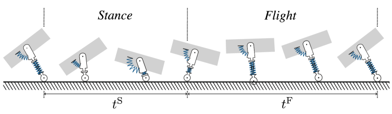
Figure 2: Visualization of an optimal hopping gait $\mathsf{g}_{0}$ at an average speed of $v_{\mathrm{avg}}=1\,\sqrt{l_{\circ}g}$, and optimal leg stiffness $k_{\mathrm{l}}^{\star}=4.44\,m_{\circ}g/l_{\circ}$. The gait begins in Stance, when the monoped’s foot touches the ground, followed by a flight phase that starts when the foot loses contact with the ground. During Flight, ground contact is assumed impossible.

This optimal gait with optimal leg stiffness $\mathsf{g}_{0}$ provides a good initial guess when solving an NLP $\widetilde{\mathcal{S}}$ for a neighboring forward speed and leg stiffness. The resulting gait can then be used to explore neighboring gaits. If in each iteration sufficiently close parameters are selected. the iterative process will, in most cases, converge, as the initial guesses are always close to the sought solutions [48].

We construct a fine grid of leg stiffness values, spanning $1\,m_{\circ}g/l_{\circ}$ to $13\,m_{\circ}g/l_{\circ}$ in increments of $\Delta k_{\mathrm{l}}=0.1\,m_{\circ}g/l_{\circ}$, and average forward speeds from $0.14\,\sqrt{l_{\circ}g}$ to $1.4\,\sqrt{l_{\circ}g}$ with a step size of $\Delta v_{\mathrm{avg}}=0.01\,\sqrt{l_{\circ}g}$, and iteratively solve the NLP $\widetilde{\mathcal{S}}$ for each grid point, starting from $\mathsf{g}_{0}$. Depending on the direction of exploration, our method can identify different local minima at each grid point. To avoid converging to unwanted local minima, grid points with existing solutions are re-checked starting from different neighboring points, and the best solution is retained. This grid-based exploration incrementally finds and refines the solution space, serving to generate an extensive library of optimal gaits.

For each average forward speed on the grid, we identify the leg stiffness that minimizes the cost of transport, defining a family of optimal gaits with adaptive leg stiffness across various speeds, denoted as $\mathcal{A}$. To evaluate the performance of $\mathcal{A}$, we compare it to a family of gaits with a constant leg stiffness, $\mathcal{C}$. For $\mathcal{C}$, the fixed leg stiffness is chosen as the mean of the stiffness values in $\mathcal{A}$.

IV RESULTS

Fig. 3 illustrates the generated grid of optimal gaits along with the two selected families, $\mathcal{A}$ and $\mathcal{C}$.

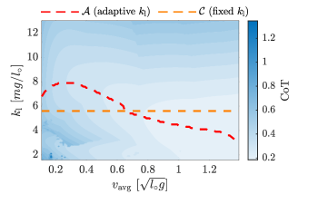
Figure 3: Top view of the map of optimal gaits generated using the grid based exploration in the $(v_{\mathrm{avg}},k_{\mathrm{l}})$ parameter space. Each point represents an optimal gait, with its color indicating the corresponding cost of transport. The families of gaits $\mathcal{A}$ (optimal leg stiffness) and $\mathcal{C}$ (constant leg stiffness) are shown respectively in red and orange.

For slower gaits, lower stiffness values generally result in a higher CoT, while at faster gaits, the CoT tends to increase with higher leg stiffness values. This trend is also reflected in the curve $\mathcal{A}$, which tends to decrease as the average speed increases. These observations align with the established concept that, at lower speeds a stiffer leg enables more efficient locomotion, whereas compliance gains significance at higher speeds. Additionally, the region surrounding $\mathcal{A}$ is relatively flat, indicating minimal variation in cost when selecting a stiffness value slightly different from the optimal.

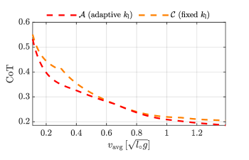
Figure 4: Comparison of the cost of transport for the family of gaits $\mathcal{A}$ with optimal stiffness and the family of gaits $\mathcal{C}$ with constant stiffness over various average forward speeds.

Fig. 4 compares the cost of transport for the families of gaits $\mathcal{A}$ and $\mathcal{C}$ across varying average forward speeds. The two curves remain closely aligned, with the most significant increase in cost of transport observed at approximately $v_{\mathrm{avg}}\approx 0.3\sqrt{l_{\circ}g}$, where the cost of transport rises by $20\%$. Averaged across all speeds, the cost of transport increases by $6\%$ with constant leg stiffness. Notably, the curves nearly overlap in the speed range $v_{\mathrm{avg}}\in[0.6,0.8]$, indicating that adapting the leg stiffness has little impact on the cost in this region.

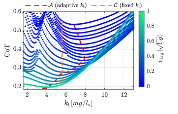
Figure 5: Zoomed-in side view of the map of optimal gaits, showing different slices of constant $v_{\mathrm{avg}}$.

Fig. 5 depicts the side view of the map of optimal gaits, showing a sampled set of slices of equal speed from the generated grid. Most depicted slices have the shape of a parabolic curve, with many showing the presence of two consecutive parabolic shapes, and hence two minima. When solving the NLP $\mathcal{S}$, where $k_{\mathrm{l}}$ is a decision variable, the optimizer might land in either of the minima, showcasing the existence of multiple local minima in such optimization problems.

The curve for $\mathcal{A}$ connects the lowest minima of these slices at each considered speed. At lower stiffness values, the slices exhibit a relatively high curvature, indicating a high sensitivity to changes in stiffness within that range. However, at higher stiffness values, the curvatures are small, indicating lower sensitivity to leg stiffness. Additionally, at lower stiffness values, slices appear organized, with slower gaits having a higher CoT. Starting from $k_{\mathrm{l}}\approx 9\,m_{\circ}g/l_{\circ}$, we observe an intertwined structure (in this 2-D view), where, as stiffness increases, slower gaits have a lower cost. However, gaits with medium speeds gradually surpass those of higher speeds.

V DISCUSSION AND CONCLUSIONS

The results suggest a correlation between leg stiffness and speed in the energy economy of a one-legged hopper. While adapting leg stiffness to the robot’s speed may provide energy savings of up to $20\%$ at certain speeds, the overall improvement in energy efficiency for a one-legged hopper with adaptive leg stiffness is modest compared to a well-chosen fixed stiffness. Although this improvement provides a compelling enough argument for implementing variable stiffness in some cases, the practical challenges of doing so—including additional energy consumption, higher costs, and the need for sophisticated control strategies—often outweigh the modest gains in efficiency. A carefully chosen constant stiffness can achieve similar results in most scenarios.

Despite the extensive computing efforts used to generate the library of optimal gaits, there is no guarantee that these solutions are global minima, showcasing the complexity of the task. Moreover, the current study was limited to explore speeds of up to $v_{\mathrm{avg}}=1.45$. Furthermore, regular manual sanity checks were required to avoid undesirable minima during the exploration process.

Future work will address these challenges by refining the optimization problem formulation and improving the grid exploration methodology to ensure a broader and more reliable search for globally optimal solutions.

References

- [1] C. Bellicoso, M. Bjelonic, L. Wellhausen, K. Holtmann, F. Günther, M. Tranzatto, P. Fankhauser, and M. Hutter, “Advances in real world applications for legged robots,” Journal of Field Robotics, vol. 35, pp. 1311–1326, 2018.
- [2] J. Delmerico, S. Mintchev, A. Giusti, et al., “The current state and future outlook of rescue robotics,” Journal Of Field Robotics, vol. 36, pp. 1171–1191, 2019.
- [3] I. Miller, F. Cladera, A. Cowley, S. Shivakumar, E. Lee, L. Jarin-Lipschitz, A. Bhat, N. Rodrigues, A. Zhou, A. Cohen, A. Kulkarni, J. Laney, C. Taylor, and V. Kumar, “Mine tunnel exploration using multiple quadrupedal robots,” IEEE Robotics And Automation Letters, vol. 5, pp. 2840–2847, 2020.
- [4] S. Kim and P. Wensing, “Design of dynamic legged robots,” Foundations And Trends In Robotics, vol. 5, pp. 117–190, 2017.
- [5] N. Kong, “Increasing reliability of legged robots in the presence of uncertainty,” Ph.D. dissertation, Carnegie Mellon University, 2023.
- [6] N. Smit-Anseeuw, R. Gleason, R. Vasudevan, and C. Remy, “The energetic benefit of robotic gait selection2̆014a case study on the robot ram¡italic¿one¡/italic¿,” IEEE Robotics and Automation Letters, vol. 2, pp. 1124–1131, 2017.
- [7] G. Fadini, T. Flayols, A. Del Prete, N. Mansard, and P. Soueres, “Computational design of energy-efficient legged robots: Optimizing for size and actuators,” in 2021 IEEE International Conference On Robotics And Automation, 2021, pp. 9898–9904.
- [8] K. Koutsoukis and E. Papadopoulos, “On the effect of robotic leg design on energy efficiency,” in 2021 IEEE International Conference On Robotics And Automation, 2021, pp. 9905–9911.
- [9] N. Kashiri, A. Abate, S. Abram, A. Albu-Schaffer, P. Clary, M. Daley, S. Faraji, R. Furnemont, M. Garabini, H. Geyer, A. Grabowski, J. Hurst, J. Malzahn, G. Mathijssen, D. Remy, W. Roozing, M. Shahbazi, S. Simha, J. Song, N. Smit-Anseeuw, S. Stramigioli, B. Vanderborght, Y. Yesilevskiy, and N. Tsagarakis, “An overview on principles for energy efficient robot locomotion,” Frontiers In Robotics And AI, vol. 5, p. 129, 2018.
- [10] H. Geyer, A. Seyfarth, and R. Blickhan, “Compliant leg behaviour explains basic dynamics of walking and running,” Book. Biological Sciences, vol. 273, pp. 2861–2867, 2006.
- [11] Z. Gan, T. Wiestner, M. Weishaupt, N. Waldern, and C. David Remy, “Passive dynamics explain quadrupedal walking, trotting, and tölting,” Journal Of Computational And Nonlinear Dynamics, vol. 11, pp. 0 210 081–2 100 812, 2016.
- [12] W. Xi, Y. Yesilevskiy, and C. Remy, “Selecting gaits for economical locomotion of legged robots,” The International Journal Of Robotics Research, vol. 35, pp. 1140–1154, 2016.
- [13] W. J. Schwind and D. E. Koditschek, “Spring loaded inverted pendulum running: a plant model,” 1998. [Online]. Available: https://api.semanticscholar.org/CorpusID:116186304
- [14] A. Struzik, K. Karamanidis, A. Lorimer, J. Keogh, and J. Gajewski, “Application of leg, vertical, and joint stiffness in running performance: A literature overview,” Applied Bionics And Biomechanics, vol. 2021, p. 9914278, 2021.
- [15] F. Meyer, M. Falbriard, K. Aminian, and G. Millet, “Vertical and leg stiffness modeling during running: Effect of speed and incline,” International Journal Of Sports Medicine, vol. 44, pp. 673–679, 2023.
- [16] D. Ferris and C. Farley, “Interaction of leg stiffness and surfaces stiffness during human hopping,” Journal Of Applied Physiology (Bethesda, Md. : 1985), vol. 82, pp. 15–22; discussion 13–4, 1997.
- [17] A. Kerdok, A. Biewener, T. McMahon, P. Weyand, and H. Herr, “Energetics and mechanics of human running on surfaces of different stiffnesses,” Journal Of Applied Physiology (Bethesda, Md. : 1985), vol. 92, pp. 469–478, 2002.
- [18] J. Morin, G. Dalleau, H. Kyröläinen, T. Jeannin, and A. Belli, “A simple method for measuring stiffness during running,” Journal Of Applied Biomechanics, vol. 21, pp. 167–180, 2005.
- [19] M. Brughelli and J. Cronin, “Influence of running velocity on vertical, leg and joint stiffness: modelling and recommendations for future research,” Sports Medicine (Auckland, N.Z.), vol. 38, pp. 647–657, 2008.
- [20] Z. Gan, Y. Yesilevskiy, P. Zaytsev, and C. Remy, “All common bipedal gaits emerge from a single passive model,” Journal Of The Royal Society, Interface, vol. 15, 2018.
- [21] T. McMahon and G. Cheng, “The mechanics of running: how does stiffness couple with speed?” Journal Of Biomechanics, vol. 23 Suppl 1, pp. 65–78, 1990.
- [22] H. Hong, S. Kim, C. Kim, S. Lee, and S. Park, “Spring-like gait mechanics observed during walking in both young and older adults,” Journal Of Biomechanics, vol. 46, pp. 77–82, 2013.
- [23] B. Serpell, N. Ball, J. Scarvell, and P. Smith, “A review of models of vertical, leg, and knee stiffness in adults for running, jumping or hopping tasks,” Journal of Sports Sciences, vol. 30, pp. 1347–1363, 2012.
- [24] R. Blickhan, “The spring-mass model for running and hopping,” Journal of Biomechanics, vol. 22, pp. 1217–1227, 1989.
- [25] R. Alexander, A model of bipedal locomotion on compliant legs, 1992, vol. 338.
- [26] M. Srinivasan, “Fifteen observations on the structure of energy-minimizing gaits in many simple biped models,” Journal Of The Royal Society, Interface, vol. 8, pp. 74–98, 2011.
- [27] R. Schroeder and A. Kuo, “Elastic energy savings and active energy cost in a simple model of running,” PLoS Computational Biology, vol. 17, p. e1009608, 2021.
- [28] Z. Shen and J. Seipel, “Animals prefer leg stiffness values that may reduce the energetic cost of locomotion,” Journal of Theoretical Biology, vol. 364, pp. 433–438, 2015.
- [29] H. Vu, R. PFEIFER, F. Iida, and X. Yu, “Improving energy efficiency of hopping locomotion by using a variable stiffness actuator,” IEEE/ASME Transactions On Mechatronics, p. 1, 2015.
- [30] X. Zhang, H. Yi, J. Liu, Q. Li, and X. Luo, “A bio-inspired compliance planning and implementation method for hydraulically actuated quadruped robots with consideration of ground stiffness,” Sensors (Basel, Switzerland), vol. 21, 2021.
- [31] N. Tsagarakis, S. Morfey, G. Medrano Cerda, L. Zhibin, and D. Caldwell, “Compliant humanoid coman: Optimal joint stiffness tuning for modal frequency control,” in 2013 IEEE International Conference On Robotics And Automation (ICRA 2013), 2013, pp. 673–678.
- [32] J. Rummel, Y. Blum, and A. Seyfarth, “Robust and efficient walking with spring-like legs,” Bioinspiration & Biomimetics, vol. 5, p. 046004, 2010.
- [33] M. Ahmadi and M. Buehler, “The arl monopod ii running robot: control and energetics,” in 1999 IEEE International Conference On Robotics And Automation, 1999, pp. 1689–1694.
- [34] M. Aboufazeli, A. Samare Filsoofi, J. Gurney, S. Meek, and V. Mathews, “An online learning algorithm for adapting leg stiffness and stride angle for efficient quadruped robot trotting,” Frontiers In Robotics And AI, vol. 10, p. 1127898, 2023.
- [35] E. Heijmink, A. Radulescu, B. Ponton, et al., “Learning optimal gait parameters and impedance profiles for legged locomotion,” in 2017 IEEE-RAS 17th International Conference On Humanoid Robotics (Humanoids), 2017, pp. 339–346.
- [36] K. Galloway, J. Clark, and D. Koditschek, “Design of a multi-directional variable stiffness leg for dynamic running,” in Mechanics Of Solids And Structures, 2008, pp. 73–80.
- [37] ——, “Variable stiffness legs for robust, efficient, and stable dynamic running,” Journal Of Mechanisms And Robotics, vol. 5, 2013.
- [38] J. Hurst and A. Rizzi, “Series compliance for an efficient running gait,” IEEE Robotics & Automation Magazine, vol. 15, pp. 42–51, 2008.
- [39] C. Remy, “Optimal exploitation of natural dynamics in legged locomotion,” Ph.D. dissertation, ETH Zurich, 2011.
- [40] M. Raff, N. Rosa, and C. Remy, “Generating families of optimally actuated gaits from a legged system’s energetically conservative dynamics,” in 2022 IEEE/RSJ International Conference On Intelligent Robots And Systems (IROS), 2022, pp. 8866–8872.
- [41] N. Rosa, B. Katamish, M. Raff, and C. D. Remy, “An approach for generating families of energetically optimal gaits from passive dynamic walking gaits,” in 2023 IEEE/RSJ International Conference on Intelligent Robots and Systems (IROS). IEEE, 2023, pp. 8551–8557.
- [42] A. Hof, “Scaling gait data to body size,” Gait & Posture, vol. 4, pp. 222–223, 1996.
- [43] C. Remy, K. Buffinton, and R. Siegwart, “Comparison of cost functions for electrically driven running robots,” in 2012 IEEE International Conference On Robotics And Automation, 2012, pp. 2343–2350.
- [44] M. Kelly, “An introduction to trajectory optimization: How to do your own direct collocation,” SIAM Review, vol. 59, no. 4, pp. 849–904, 2017.
- [45] J. A. E. Andersson, J. Gillis, G. Horn, J. B. Rawlings, and M. Diehl, “CasADi – A software framework for nonlinear optimization and optimal control,” Mathematical Programming Computation, 2018.
- [46] A. Wächter and L. T. Biegler, “On the implementation of an interior-point filter line-search algorithm for large-scale nonlinear programming,” Mathematical programming, vol. 106, pp. 25–57, 2006.
- [47] P. R. Amestoy, I. S. Duff, J.-Y. L’Excellent, and J. Koster, “A fully asynchronous multifrontal solver using distributed dynamic scheduling,” SIAM Journal on Matrix Analysis and Applications, vol. 23, no. 1, pp. 15–41, 2001.
- [48] E. L. Allgower and K. Georg, Introduction to numerical continuation methods. SIAM, 2003.