Performance of Practical Quantum Oblivious Key Distribution

Abstract

Motivated by the applications of secure multiparty computation as a privacy-protecting data analysis tool, and identifying oblivious transfer as one of its main practical enablers, we propose a practical realization of randomized quantum oblivious transfer. By using only symmetric cryptography primitives to implement commitments, we construct computationally-secure randomized oblivious transfer without the need for public-key cryptography or assumptions imposing limitations on the adversarial devices. We show that the protocol is secure under an indistinguishability-based notion of security and demonstrate an experimental implementation to test its real-world performance. Its security and performance are then compared to both quantum and classical alternatives, showing potential advantages over existing solutions based on the noisy storage model and public-key cryptography.

1 Introduction

Cryptography is a critical tool for data privacy, a task deeply rooted in the functioning of today’s digitalized world. Whether it is in terms of secure communication over the Internet or secure data access through authentication, finding ways of protecting sensitive data is of utmost importance. The one-time pad encryption scheme allows communication with perfect secrecy [1], at the cost of requiring the exchange of single-use secret (random) keys of the size of the communicated messages. Distribution of secret keys, therefore, is considered one of the most important tasks in cryptography. Modern cryptography relies heavily on conjectures about the computational hardness of certain mathematical problems to design solutions for the key distribution problem. However, as quantum computers threaten to make most of the currently used cryptography techniques obsolete [2], better solutions for data protection are needed. This transition towards quantum-resistant solutions becomes particularly crucial when it comes to protecting data associated with the government, finance and health sectors, being already susceptible to intercept-now-decrypt-later attacks.

Cryptography solutions secure in a post-quantum world, where large-scale quantum computers will be commercially available, have been explored in two directions. Classical cryptography based solutions, also referred as post-quantum cryptography [3, 4, 5], involve using a family of mathematical problems that are conjectured to be resilient to quantum computing attacks. On the other hand, quantum cryptography based solutions [6] using the laws of quantum mechanics can offer information-theoretic security, depending on the physical properties of quantum systems rather than computational hardness assumptions. Quantum Key Distribution (QKD) [7] is the most well-studied and developed of these quantum solutions, while other works beyond QKD have been proposed [8].

It is noteworthy that secure communication is not the only cryptographic task where end-users’ private data may be exposed to an adversary. Cryptography beyond secure communication and key distribution includes zero-knowledge proofs, secret sharing, contract signing, bit commitment (BC), e-Voting, secure data mining, etc. [9]. A huge class of such problems can be cast as Multi-Party Computation (MPC), where distrustful parties can benefit from a joint collaborative computation on their private inputs. It requires parties’ individual inputs to remain hidden from each other during the computation, among other security guarantees such as correctness, fairness, etc. [10]. Secure MPC is a powerful cryptographic tool with a vast range of applications as it allows collaborative work with private data. Generic MPC protocols work by expressing the function to evaluate as an arithmetic or Boolean circuit and then securely evaluating the individual gates. These protocols are based on one of two main fundamental primitives[11, 12, 13, 14]: Oblivious Transfer (OT) and Homomorphic encryption, the former of which is the focus of this work.

A 1-out-of-2 OT [15], is the task of sending two messages, such that the receiver can choose only one message to receive, while the sender remains oblivious to this choice. The original protocol, now called all-or-nothing OT, was proposed by Rabin in 1981 [16], where a single message is sent and the receiver obtains it with 1/2 probability. The two flavours of OT were later shown to be equivalent [17]. Notably, it has been shown that it is possible to implement secure MPC using only OT as a building block [18, 19]. Relevant to our work is a variation of OT called Random Oblivious Transfer (ROT), which is similar to 1-out-of-2 OT, except that both the sent messages and the receiver’s choice are randomly chosen during the execution of the protocol. This can be seen as analogous to the key distribution task, in which both parties receive a random message (the key) as output. By appropriately encrypting messages using the outputs of a ROT protocol as a shared resource, it is possible to efficiently perform 1-out-of-2 OT. As an important consequence, parties expecting to engage in MPC in the future can execute many instances of ROT in advance and save the respective outputs as keys to be later used as a resource to perform fast OTs during an MPC protocol [20]. Because of this, we can think of ROT as a basic primitive for secure MPC.

In the context of quantum cryptography, OT is remarkable because, unlike classically, there exists a reduction from OT to commitment schemes [21, 22, 23]. This result is somewhat undermined by the existence of several theorems regarding the impossibility of unconditionally secure commitments both in classical [24] and quantum [25, 26] cryptography, and it was further proven impossible in the more general abstract cryptography framework [27]. These results, in turn, imply that unconditionally secure OT itself is impossible. In light of this, approaches with different technological or physical constraints on the adversarial power have been proposed. Practical solutions based on hardware limitations, such as bounded and noisy storage [28, 29, 30, 31], have the disadvantage that the performance of such protocols decreases as technology improves.

Computationally-secure classical protocols have also been proposed [32, 33, 34, 35], which work under the assumptions of post-quantum public-key cryptography. Alternatively, we can take advantage of quantum reduction from OT to commitments by implementing commitment schemes using (non-trapdoor) one-way functions (OWF) such as Hash functions [36] and pseudo-random generators [37] which allows us to construct OT from symmetric cryptography primitives. The existence of general OWFs is a weaker assumption than public-key cryptography [38, 39], which requires the existence of the more restrictive trapdoor OWFs. This difference is significant, as the latter are defined over mathematically rich structures, such as elliptic curves and lattices, and the computational hardness of the associated problems is less understood than that of their private-key counterparts. For an in-depth study of the relation between OT and OWFs see [40].

Having established that there is a theoretical merit in using computationally-secure quantum protocols to implement secure MPC, it is also important to understand how practical quantum protocols compare with currently used classical solutions in security, computational and communication complexity, and practical speed in current setups. This work focuses in studying the performance of a practical quantum ROT protocol and its potential advantages compared to currently used classical solutions for OT during MPC.

The contributions of this work can be summarized as follows: We introduce a definition for a quantum ROT protocol, satisfying a strong indistinguishability-based security notion, which generalizes the security of classical ROT protocols. We present a protocol that realizes said quantum ROT, based on the standard commitment-based construction (originally by [41, 21]). The protocol uses a weakly-interactive string commitment scheme which is statistically binding and computationally hiding, and can be implemented in practice using current QKD setups. We present a formal finite-key security proof of the proposed protocol assuming only the existence of quantum-secure OWFs, together with security bounds as functions of the protocol’s parameters. We also present calculations for the maximum usable channel error, as well as for the key rate as a function of the number of shared signals per instance of the protocol. We experimentally demonstrate our protocol using current technology with a setup based on polarization-entangled photons. We also present a security analysis which accounts for potential implementation-specific attacks and how they can be circumvented using an appropriate reporting strategy. Finally, we compare our performance results with the performance of current ROT solutions and point out the advantages and disadvantages of using quantum ROT in the context of MPC.

2 Preliminaries

2.1 Quantum computational efficiency and distinguishability

A quantum program is defined as a set of instructions to be run in a specified type of quantum computer, which are devices that have a classical interface and a quantum part. Quantum programs can be compared with probabilistic classical programs as they both have natural numbers as inputs/outputs. When a quantum computer runs the program $T$ with input $x\in\mathbb{N}$, we assume that the quantum part of the computer starts with some predefined initial state, performs a sequence of operations on its quantum registers, and upon halting, it outputs $T(x)\in\mathbb{N}$ on its classical interface by reading the appropriate registers associated with the program’s output.

Definition 2.1.

(Computational efficiency)
Let $T$ be a quantum program. We say that $T$ is computationally efficient (or polynomial-time) if there exists a polynomial $P$ such that the running time of $T(x)$ is $O(P(x))$.

Definition 2.2.

(Distinguishing Advantage)
Let $X_{1},X_{2}$ be two random variables with values in $\mathbb{N}$. For any quantum program $T$, the distinguishing advantage of $X_{1},X_{2}$ using $T$ is defined as

$$\textnormal{Adv}_{T}(X_{1},X_{2})=\big{|}\Pr[T(X_{1})=1]-\Pr[T(X_{2})=1]\big{|},$$ (1)

Analogously, let $\rho_{1},\rho_{2}\in\mathcal{D}(\mathcal{H})$. For any quantum program $T$, the distinguishing advantage of $\rho_{1},\rho_{2}$ using $T$ is defined as

$$\textnormal{Adv}_{T}(\rho_{1},\rho_{2})=\big{|}\Pr[T^{(\rho_{1})}=1]-\Pr[T^{(\rho_{2})}=1]\big{|},$$ (2)

where $T^{(\rho)}$ denotes the classical output of the program starting with the quantum state $\rho$ and zero classical input.

Definition 2.3.

(Indistinguishability - Finite)
Let $\rho_{1},\rho_{2}\in\mathcal{D}(\mathcal{H})$ and $\varepsilon\geq 0$. We say that $\rho_{1}$ and $\rho_{2}$ are $\varepsilon$-indistinguishable, denoted by $\rho_{1}\approx_{\varepsilon}\rho_{2}$, whenever

$$\textnormal{Adv}_{T}\big{(}\rho_{1},\rho_{2}\big{)}\leq\varepsilon\quad\textnormal{for all quantum programs }T.$$ (3)

$\varepsilon$-indistinguishability for random variables is defined analogously.

As the following proposition states, to show that two states are $\varepsilon$-indistinguishable, it is enough to upper bound their trace distance $D$. (for more detail on the relationship of these quantities, see [42, 43]).

Proposition 2.1.

For any pair of quantum states $\rho_{1},\rho_{2}\in\mathcal{D}(\mathcal{H})$ it holds that

$$\rho_{1}\approx_{D(\rho_{1},\rho_{2})}\rho_{2}.$$ (4)

Definition 2.4.

(Indistinguishability - Asymptotical)
Let $\{\rho_{1}^{(k)}\in\mathcal{D}(\mathcal{H}_{k})\}$ and $\{\rho_{2}^{(k)}\in\mathcal{D}(\mathcal{H}_{k})\}$ be two families of density operators. We say that the two families are statistically indistinguishable if there exists a negligible function $\varepsilon(k)\geq 0$ such that

$$\rho_{1}^{(k)}\approx_{\varepsilon(k)}\rho_{2}^{(k)}\quad\textnormal{for all }k\in\mathbb{N}.$$ (5)

Furthermore, we say the two families are computationally indistinguishable if for every efficient quantum program $T$, there exists a negligible function $\varepsilon_{T}(k)\geq 0$ such that

$$\textnormal{Adv}_{T}\big{(}\rho_{1}^{(k)},\rho_{2}^{(k)}\big{)}\leq\varepsilon_{T}(k)\quad\textnormal{for all }k\in\mathbb{N}.$$ (6)

Statistical and computational indistinguishability for random variables is defined analogously.

For the purposes of this work, the concept of indistinguishability will be often used to compare the state of systems in a “real” run of the protocol versus another “ideal” desired state. In those cases, the associated families of states are parameterized by the protocol’s security parameters. When the associated families $\{\rho_{1}^{(k)}\}$ and $\{\rho_{2}^{(k)}\}$ are clear by context, we will just refer to them as $\rho_{1}$ and $\rho_{2}$ and use the following notation to denote indistinguishability:

$$\rho_{1}\approx\rho_{2}$$ for statistically indistinguishable

$$\rho_{1}\approx^{(c)}\rho_{2}$$ for computationally indistinguishable

Additionally, in this work we consider protocols that can abort if certain conditions are satisfied. Mathematically, it is useful to consider the state of the aborted protocol as the zero operator. This means that events that trigger the protocol to abort are described as trace-decreasing operations, and hence, the operator representing the associated system at the end of the protocol is, in general, not normalized. The probability of the protocol finishing successfully is given then by the trace of the final state of the output registers. Note that the above definitions of indistinguishability can be naturally extended to non-normalized operators since the outcomes of a quantum program can always be represented by the outcomes of a POVM $\{F_{i}\}$, whose probabilities are given by $\Tr[F_{i}\rho]$, which is a well defined quantity even for non-normalized $\rho$. We now turn our attention to the properties of indistinguishable states. It is worth noting that computational indistinguishability is only meaningful in terms of information security when the adversary is assumed to have limited computational capabilities. It is important then to define the type of quantum operations such adversary can perform:

Definition 2.5.

(Efficient quantum operation)
We say that a family $\{\mathcal{E}^{(k)}\}_{k=1}^{\infty}$ of quantum operations is efficient if there exists an efficient quantum program $T$ such that, for each $k$, $\mathcal{E}^{(k)}$ is the associated operation applied to the quantum part of the machine while running $T$ on input $k$

The following properties are straightforward to prove from Definitions 2.3 and 2.4 and the properties of trace distance:

Lemma 2.1.

(Properties of indistinguishable states I)
Let $\rho_{1},\rho_{2},\rho_{3}\in\mathcal{D}(\mathcal{H})$:

1. $\rho_{1}\approx_{\varepsilon}\rho_{2}\wedge\rho_{2}\approx_{\varepsilon^{\prime}}\rho_{3}\Rightarrow\rho_{1}\approx_{\varepsilon+\varepsilon^{\prime}}\rho_{3}$

2. $\rho_{1}\approx_{\varepsilon}\rho_{2}\wedge\sigma_{1}\approx_{\varepsilon^{\prime}}\sigma_{2}\Rightarrow\rho_{1}\otimes\sigma_{1}\approx_{\varepsilon+\varepsilon^{\prime}}\rho_{2}\otimes\sigma_{2}$

3. Let $x\in\mathcal{X}$. For any probability distribution $P_{x}$, assume that $\big{(}\forall x\in\mathcal{X}\big{)}\>\rho_{1}^{x}\approx_{\varepsilon^{x}}\rho_{2}^{x}$. Then

   $$\sum_{x\in\mathcal{X}}P_{x}\rho_{1}^{x}\approx_{\varepsilon^{\textnormal{max}}}\sum_{x\in\mathcal{X}}P_{x}\rho_{2}^{x}\>\>\textnormal{where}\>\>\varepsilon^{\textnormal{max}}=\max_{x\in\mathcal{X}}\{\varepsilon^{x}\}.$$

4. $\rho_{1}\approx_{\varepsilon}\rho_{2}\Rightarrow\mathcal{E}(\rho_{1})\approx_{\varepsilon}\mathcal{E}(\rho_{2})$, for any completely positive, trace non-increasing map $\mathcal{E}$.

Lemma 2.2.

(Properties of indistinguishable states II)
Let $\{\rho_{1}(k)\},\{\rho_{2}(k)\},\{\rho_{3}(k)\}$ be families of density operators parameterized by $k=1,2,\ldots$ The following statements hold for asymptotic computational indistinguishability:

1. $\rho_{1}\approx^{(c)}\rho_{2}\wedge\rho_{2}\approx^{(c)}\rho_{3}\Rightarrow\rho_{1}\approx^{(c)}\rho_{3}$

2. $\rho_{1}\approx^{(c)}\rho_{2}\wedge\sigma_{1}\approx^{(c)}\sigma_{2}\Rightarrow\rho_{1}\otimes\sigma_{1}\approx^{(c)}\rho_{2}\otimes\sigma_{2}$

3. Let $x\in\mathcal{X}$. For any probability distribution $P_{x}$, assume that $\big{(}\forall x\in\mathcal{X}\big{)}\>\rho_{1}^{x}\approx^{(c)}\rho_{2}^{x}$. Then

   $$\sum_{x\in\mathcal{X}}P_{x}\rho_{1}^{x}\approx^{(c)}\sum_{x\in\mathcal{X}}P_{x}\rho_{2}^{x}.$$

4. $\rho_{1}\approx^{(c)}\rho_{2}\Rightarrow\mathcal{E}(\rho_{1})\approx^{(c)}\mathcal{E}(\rho_{2})$, where $\{\mathcal{E}^{(k)}\}$ is an efficient family of quantum operations acting on the respective $\rho_{i}(k)$.

2.2 Entropic quantities

We start off by defining a useful pair of quantities for measuring information in quantum systems: the max-entropy and the conditional min-entropy. The max entropy is a measure of the number of possible different outcomes that can result from measuring a quantum state, whereas the conditional min-entropy is a way of measuring the information that a party can infer from a quantum system given access to another correlated quantum system. This measures will be useful to bound the distance between states based on their internal correlations.

Definition 2.6.

(Max-entropy)
Let $\rho\in\mathcal{D}(\mathcal{H})$. The max-entropy of $\rho$ is defined as

$$H_{\max}(\rho)=\log\big(\dim(\textnormal{supp}(\rho))\big{missing}),$$ (7)

where $\textnormal{supp}(\rho)$ denotes the support subspace of $\rho$ and $\dim$ denotes its dimension.

Definition 2.7.

(Min-entropy and conditional min-entropy)
Let $\rho\in\mathcal{D}(\mathcal{H})$ and $\lambda_{\max}(\rho)$ denote the maximum eigenvalue of $\rho$. The min-entropy of $\rho$ is defined as

$$H_{\textnormal{min}}(\rho)=-\log(\lambda_{\max}(\rho)),$$ (8)

Let $\rho_{AB}\in\mathcal{D}(\mathcal{H}_{A}\otimes\mathcal{H}_{B})$ and $\sigma_{B}\in\mathcal{D}(\mathcal{H}_{B})$. The conditional min-entropy of $\rho_{AB}$ given $\sigma_{B}$ is defined as

$$H_{\textnormal{min}}(\rho_{AB}|\sigma_{B})=-\log(\lambda_{\sigma_{B}}),$$ (9)

where $\lambda_{\sigma_{B}}$ is the minimum real number such that $\lambda_{\sigma_{B}}(\mathbb{1}_{A}\otimes\sigma_{B})-\rho_{AB}$ is non-negative. The conditional min-entropy of $\rho_{AB}$ given $\mathcal{H}_{B}$ is defined as

$$H_{\textnormal{min}}(A|B)_{\rho}=\!\!\!\!\!\!\sup_{\sigma_{B}\in\mathcal{D}(\mathcal{H}_{B})}\!\!\!\!\!\!H_{\textnormal{min}}(\rho_{AB}|\sigma_{B}),$$ (10)

Furthermore, let $\varepsilon>0$. The $\varepsilon$-smooth conditional min-entropy is defined as

$$H_{\textnormal{min}}^{\varepsilon}(A|B)_{\rho}=\!\!\!\!\!\!\!\!\!\sup_{\rho^{\prime}_{AB}\in\mathcal{B}^{\varepsilon}(\rho_{AB})}\!\!\!\!\!\!\!\!\!H_{\textnormal{min}}(A|B)_{\rho^{\prime}},$$ (11)

where $\mathcal{B}^{\varepsilon}(\rho_{AB})=\{\rho^{\prime}_{AB}:D(\rho_{AB},\rho^{\prime}_{AB})<\varepsilon\}$.

The smooth conditional min-entropy is in general hard to compute. Because of this, it is useful to have some tools to bound it for states that have some specific forms. In our case we are interested in states that are partially classical.

Definition 2.8.

(Partially classical states)
A quantum state described by the density operator $\rho_{AB}\in\mathcal{D}(\mathcal{H}_{A}\otimes\mathcal{H}_{B})$ is classical in $\mathcal{H}_{A}$ (or classical in $A$) if it can be written in the form

$$\rho_{AB}=\sum_{x}\lambda_{x}|x\rangle\ \!\!\!\langle x|_{A}\otimes\rho^{x}_{B},$$ (12)

where the set $\{{|{x}\rangle}\}_{x}$ is an orthonormal basis for $\mathcal{H}_{A}$. A multipartite state is said to be classical if it is classical in all its parts.

When dealing with partially classical states as shown in Eq. (12), we will refer to the operators $\rho^{x}_{B}$ as the state of the system $B$ conditioned to $x$.

Lemma 2.3.

(Properties of min-,max-entropy)
Let $\varepsilon,\varepsilon^{\prime}\geq 0$:

1. $H_{\textnormal{min}}(\rho_{A}\otimes\rho_{B}|\rho_{B})=-\log(\lambda_{\max}(\rho_{A}))$

2. $H_{\textnormal{min}}^{\varepsilon+\varepsilon^{\prime}}(AA^{\prime}|BB^{\prime})_{\rho\otimes\rho^{\prime}}\geq H_{\textnormal{min}}^{\varepsilon}(A|B)_{\rho}+H_{\textnormal{min}}^{\varepsilon^{\prime}}(A^{\prime}|B^{\prime})_{\rho^{\prime}}$

3. $H_{\textnormal{min}}^{\varepsilon}(A|BC)_{\rho}\leq H_{\textnormal{min}}^{\varepsilon}(A|B)_{\rho}$

4. $H_{\textnormal{min}}^{\varepsilon}(AB|C)_{\rho}\leq H_{\textnormal{min}}^{\varepsilon}(A|BC)_{\rho}+H_{\max}(\rho_{B})$

5. $H_{\textnormal{min}}^{\varepsilon}(A|B)_{\rho}\geq\inf_{x}\{H_{\textnormal{min}}^{\varepsilon}(\rho_{A}^{x})\}$, whenever the state $\rho_{AB}$ is classical on $B$

We use universal hashing to implement randomness extraction in the final steps of the protocol. With the appropriate conditional min-entropy bounds provided by Lemma A.3, we can use the quantum leftover hash lemma to show that Bob can only get negligible information about at least one of the two strings. The proof both Lemmas 2.3 and 2.4 can be found in [44].

Definition 2.9.

(Universal hashing)
A set of functions $\textnormal{{F}}=\{f_{i}:\{0,1\}^{m}\rightarrow\{0,1\}^{n}\}$ is a universal hash family if, for all $x,y\in\{0,1\}^{m}$, such that $x\neq y$, and $i$ chosen uniformly at random, we have

$$\textnormal{Pr}[f_{i}(x)=f_{i}(y)]\leq\frac{1}{2^{n}}.$$

Lemma 2.4.

(Quantum leftover hash)
Let $\textnormal{{F}}=\{f_{i}:\{0,1\}^{n}\rightarrow\{0,1\}^{\ell}\}$ be a universal hash family, let $\mathcal{H}_{A},\mathcal{H}_{B},\mathcal{H}_{F},\mathcal{H}_{E}$ be Hilbert spaces such that $\{{|{x}\rangle}\}_{x\in\{0,1\}^{n}},\{{|{f_{i}}\rangle}\}_{f_{i}\in\textnormal{{F}}}$, and $\{{|{e}\rangle}\}_{e\in\{0,1\}^{\ell}}$ are orthonormal bases for $\mathcal{H}_{A},\mathcal{H}_{F},$ and $\mathcal{H}_{E}$ respectively. Then for any $\varepsilon\geq 0$ and any state of the form

$$\rho_{ABFE}=\frac{1}{|\textnormal{{F}}|}\sum_{\begin{subarray}{c}x\in\{0,1\}^{n}\\ f_{i}\in\textnormal{{F}}\end{subarray}}\lambda(x)|f_{i}\rangle\ \!\!\!\langle f_{i}|_{F}\otimes|f_{i}(x)\rangle\ \!\!\!\langle f_{i}(x)|_{E}\otimes|x\rangle\ \!\!\!\langle x|_{A}\otimes\rho^{x}_{B},$$ (13)

it holds that

$$\rho_{EBF}\approx_{\varepsilon^{\prime}}\mathsf{U}_{E}\otimes\rho_{BF}$$ (14)

with

$$\varepsilon^{\prime}=\varepsilon+\frac{1}{2}\cdot 2^{-\frac{1}{2}(H_{\textnormal{min}}^{\varepsilon}(A|B)_{\rho}-\ell)}$$ (15)

3 Quantum Random Oblivious Transfer (ROT)

We move towards defining the concept of Random Oblivious Transfer, which is the main object of study of this work. Informally, a ROT is a probabilistic protocol between a sender and a receiver, which returns two strings $m_{0},m_{1}$ to the sender, and a bit $c$, together with the string $m_{c}$ to the receiver. We say that the protocol is secure against a cheating sender if they are not able to get information of the value of $c$. Similarly, the protocol is secure against a cheating receiver if it can be guaranteed that upon finishing the protocol, they are ignorant about at least one of the two strings $m_{0},m_{1}$.

We are interested in a protocol which assumes that the parties have quantum capabilities (ability to generate entangled states and measure in different bases), hence we are concerned with security definitions which take into account the quantum information shared during the protocol execution. Let $\mathcal{H}_{C}$, $\mathcal{H}_{M_{0}}$, $\mathcal{H}_{M_{1}}$, and $\mathcal{H}_{M_{C}}$ denote the Hilbert spaces of the memory registers in which the information of the bit $c$, and the strings $m_{0},m_{1},m_{c}$, is saved. Note that here, as well as in the definitions below, the upper-case symbols $C$, $M_{0}$, $M_{1}$, and $M_{C}$ are labels of the corresponding systems, and not variables. For any Hilbert space $\mathcal{H}_{X}$, we denote the associated maximally mixed state by $\mathsf{U}_{X}$.

Definition 3.1.

(Quantum Random Oblivious Transfer)
An $n$-bit Quantum Random Oblivious Transfer with security parameter $k$ is a protocol, without external inputs, between two parties S (the sender) and R (the receiver) which, upon finishing, outputs the joint quantum state $\rho_{M_{0},M_{1},C,M_{C}}$ satisfying:

1. (Correctness) The final state of the outputs when the protocol is run with both honest parties satisfies

   $$\rho_{M_{0},M_{1},C,M_{C}}\approx\frac{p_{\textnormal{succ}}}{2^{(2n+1)}}\!\!\!\!\!\!\!\!\!\sum\limits_{\begin{subarray}{c}m_{0},m_{1}\in\{0,1\}^{n}\\ c\in\{0,1\}\end{subarray}}\!\!\!\!\!\!\!\!\!|m_{0}\rangle\ \!\!\!\langle m_{0}|_{M_{0}}\otimes|m_{1}\rangle\ \!\!\!\langle m_{1}|_{M_{1}}\otimes|c\rangle\ \!\!\!\langle c|_{C}\otimes|m_{c}\rangle\ \!\!\!\langle m_{c}|_{M_{C}},$$ (16)

   where $p_{\textnormal{succ}}=\textnormal{Tr}[\rho_{M_{0},M_{1},C,M_{C}}]$ is the probability of the protocol finishing successfully.

2. (Security against dishonest sender) Let $H_{S}$ be the Hilbert space associated to all of the sender’s memory registers. For the final state after running the protocol with an honest receiver it holds that

   $$\rho_{S,C}\approx\rho_{S}\otimes\mathsf{U}_{C}.$$ (17)

3. (Security against dishonest receiver) Let $H_{R}$ be the Hilbert space associated to all of the receiver’s memory registers. For the final state after running the protocol with an honest sender, there exists a binary probability distribution given by $(p_{0},p_{1})$ such that

   $$\rho_{R,M_{0},M_{1}}\approx\sum_{b}\left(p_{b}\,\rho_{R,M_{\bar{b}}}^{b}\otimes\mathsf{U}_{M_{b}}\right).$$ (18)

The above properties define statistical security for each feature of the ROT protocol. If any of them holds for the notion of computational indistinguishability $\approx^{(c)}$ instead, we say that the ROT protocol is computationally secure in the respective sense.

We expect the outputs $m_{0},m_{1},c$ to be uniformly distributed and the receiver always obtaining the correct corresponding $m_{c}$. The first property is typically called correctness and it states that, when both parties follow the protocol, the probability of it not aborting and having incorrect outputs is neglible in the security parameter. The probability $p_{\textnormal{succ}}$ of the protocol finishing appears explicitly in this expression as the success of quantum protocols often depends on external conditions, most notably the noise in the quantum communication channels. For any specific value of $p_{\textnormal{succ}}$ and any $\varepsilon^{r}\leq 1-p_{\textnormal{succ}}$ we say that, under the associated external conditions, the protocol is $\varepsilon^{(r)}$-robust.

The second property, called security against dishonest sender, states that regardless of how much the sender deviates from the protocol, their final quantum state (which includes all the information accessible to them) is uncorrelated to the uniformly distributed value of the receiver’s choice bit $c$. Analogously, the third property, called security against dishonest receiver, states that even for a receiver running an arbitrary program, by the end of the protocol there is always at least one of the two strings $m_{0},m_{1}$ that is completely unknown to them (denoted by $m_{b}$).

3.1 Additional schemes

In this section, we define the subroutines used inside of our main protocol. We start by defining a weakly-interactive commitment scheme, which gets its name from the fact that the verifier publishes a single random message at the start, which defines the operations that the committer performs.

Definition 3.2.

(String commitment scheme)
Let $k,n\in\mathbb{N}$. A weakly-interactive $n$-bit string commitment scheme with security parameter $k$ is a family of efficient (in $n$, as well as in $k$) programs $\mathtt{com},\mathtt{open},\mathtt{ver}$

$$\begin{split}\mathtt{com}&:\{0,1\}^{n}\times\{0,1\}^{n_{s}(k)}\times\{0,1\}^{n_{r}(k)}\rightarrow\{0,1\}^{n_{c}(k)};\\ \mathtt{open}&:\{0,1\}^{n}\times\{0,1\}^{n_{s}(k)}\rightarrow\{0,1\}^{n_{o}(k)};\\ \mathtt{ver}&:\{0,1\}^{n_{c}(k)}\times\{0,1\}^{n_{o}(k)}\times\{0,1\}^{n_{r}(k)}\rightarrow\{0,1\}^{n}\cup\{\bot\},\end{split}$$ (19)

such that

1. (correctness) $\mathtt{ver}\big{(}\mathtt{com}(m,s,r),\mathtt{open}(m,s),r\big{)}=m$ for all $m\in\{0,1\}^{n}$, $s\in\{0,1\}^{n_{s}}$, and $r\in\{0,1\}^{n_{r}}$.

2. (hiding property) For all $m_{1},m_{2}\in\{0,1\}^{n}$ and $r\in\{0,1\}^{n_{r}}$ the distributions for $\mathtt{com}(m_{1},s_{1},r)$ and $\mathtt{com}(m_{2},s_{2},r)$ are computationally (or statistically) indistinguishable in $k$ whenever $s_{1},s_{2}$ are sampled uniformly.

3. (binding property) For uniformly sampled $r$, the probability $\varepsilon_{\textnormal{bind}}(k)$ that there exists a tuple $(\textnormal{com},\textnormal{open}_{1},\textnormal{open}_{2})$ such that

   $$\bot\neq\mathtt{ver}(\textnormal{com},\textnormal{open}_{1},r)\neq\mathtt{ver}(\textnormal{com},\textnormal{open}_{2},r)\neq\bot,$$ (20)

   is negligible in $k$.

Weakly-interactive string commitment schemes can be implemented using common cryptographic primitives like hash functions or pseudo-random generators. Most notably, Naor’s commitment protocol [37] provides a black box construction of weakly-interactive commitments from OWFs.

Definition 3.3.

(Verifiable information reconciliation scheme)
Let $\mathcal{C}\subseteq\{0,1\}^{n}\times\{0,1\}^{n}$. A verifiable one-way Information Reconciliation (IR) scheme with security parameter $k$ and leak $\ell$ for $\mathcal{C}$ is a pair of efficient programs $(\mathtt{syn},\mathtt{dec})$ with

$$\begin{split}\mathtt{syn}&:\{0,1\}^{n}\rightarrow\{0,1\}^{\ell},\\ \mathtt{dec}&:\{0,1\}^{\ell}\times\{0,1\}^{n}\rightarrow\{0,1\}^{n}\cup\{\bot\},\end{split}$$ (21)

such that,

1. (correctness) Whenever $(x,y)\in\mathcal{C}$ it holds that $\mathtt{dec}(\mathtt{syn}(x),y)=x$ except with negligible probability in $k$.

2. (verifiability) For any $(x,y)\in\{0,1\}^{n}\times\{0,1\}^{n}$ it holds that either $\mathtt{dec}(\mathtt{syn}(x),y)=x$ or $\mathtt{dec}(\mathtt{syn}(x),y)=\bot$, except with negligible probability $\varepsilon_{\textnormal{IR}}(k)$.

Due to Shannon’s Noisy-channel coding theorem, the size of the leak $\ell$ for any IR scheme over a discrete memoryless channel is lower bounded by $h(p)$, where $p$ represents the bit-error probability, and $h(\cdot)$ denotes the binary entropy function. For concrete IR schemes, we can usually describe their efficiency using the ratio between the scheme’s leak and the theoretical optimal: $f=\frac{\ell}{h(p)}$.

3.2 The protocol

In this section we present the protocol $\pi_{\textnormal{QROT}}$ for an $n$-bit quantum ROT based on the primitives described in the previous section and the use of quantum communication. The protocol’s main security parameter is $N_{0}$, which corresponds to the number of quantum signals sent during the quantum phase. Additionally, it has two secondary security parameters $k,k^{\prime}$, which define the security of the underlying commitment and IR schemes, respectively.

In order to facilitate the finite-key security analysis, the description of $\pi_{\textnormal{QROT}}$ features two statistical tolerance parameters, denoted as $\delta_{1},\delta_{2}$. The role of $\delta_{1}$ is to account for the error in the estimation of the Qubit Error Rate (QBER), while the role of $\delta_{2}$ is to account for the small variations in the frequency of outcomes of $50/50$ events. These parameters can be ignored (set to zero) when considering very large values of $N_{0}$. In the following description of the protocol we use the bit values $0,1$ to the denote the computational and Hadamard bases for qubit Hilbert spaces, respectively, and ${|{\Phi^{+}}\rangle}=\frac{1}{\sqrt{2}}({|{00}\rangle}+{|{11}\rangle})$. Finally, we will use the relative (or normalized) Hamming weight function $r_{H}:\{0,1\}^{n}\rightarrow[0,1]$ defined for any $x=(x_{1},\ldots,x_{n})$ as

$$r_{\textnormal{H}}(x)=\frac{1}{n}\sum_{i=1}^{n}x_{i}.$$ (22)

Parameters:

• Parameter estimation sample ratio $0<\alpha<1$

• Statistical tolerance parameters $\delta_{1},\delta_{2}$

• Maximum qubit error rate $0\leq p_{\text{max}}\leq 1/2$

• Coincidence block size $N_{0}\in\mathbb{N}$, test set size $N_{\textnormal{test}}=\alpha N_{0}$, minimum check set size $N_{\textnormal{check}}=(\frac{1}{2}-\delta_{2})\alpha N_{0}$, and raw string block size $N_{\textnormal{raw}}=(\frac{1}{2}-\delta_{2})(1-\alpha)N_{0}$

• Weakly-interactive 2-bit string commitment scheme $(\mathtt{com},\mathtt{open},\mathtt{ver})$, which is computationally hiding and statistically binding, with security parameter $k\in\mathbb{N}$ and associated string lengths $n_{s},n_{r},n_{c},n_{o}$

• Verifiable one-way information reconciliation scheme $(\mathtt{syn},\mathtt{dec})$ on the set $\mathcal{C}=\{(x,y)\in\{0,1\}^{N_{\text{raw}}}\times\{0,1\}^{N_{\text{raw}}}:r_{\textnormal{H}}(x\oplus y)<p_{\text{max}}+\delta_{1}\}$, with security parameter $k^{\prime}\in\mathbb{N}$ and leak $\ell=f\cdot h(p_{\text{max}}+\delta_{1})$

• Universal hash family $\textnormal{{F}}=\big{\{}f_{i}:\{0,1\}^{N_{\text{raw}}}\rightarrow\{0,1\}^{n}\big{\}}_{i}$

Parties: The sender Alice and the receiver Bob.
Protocol steps:
Quantum phase

1. Alice generates the state $\bigotimes_{i=1}^{N_{0}}{|{\Phi^{+}}\rangle}_{i}$ and sends one qubit of each entangled pair to Bob through a (potentially noisy) quantum channel. Then she samples the string $\theta^{A}\in\{0,1\}^{N_{0}}$ and for each $i\in I=\{1,\ldots,N_{0}\}$ performs a measurement in the basis $\theta^{A}_{i}$ on her qubit of ${|{\Phi^{+}}\rangle}_{i}$ to obtain the outcome string $x^{A}$.

2. Bob samples the string $\theta^{B}\in\{0,1\}^{N_{0}}$ and for each $i\in I$ performs a measurement in the basis $\theta^{B}_{i}$ on his qubit of ${|{\Phi^{+}}\rangle}_{i}$ to obtain the outcome string $x^{B}$.

Commit/open phase

1. Alice uniformly samples the string $r\in\{0,1\}^{n_{r}}$ and sends it to Bob.

2. For each $i\in I$, Bob samples a random string $s_{i}\in\{0,1\}^{n_{s}}$, computes

   $$(\textnormal{com}_{i},\textnormal{open}_{i})=\big{(}\mathtt{com}((\theta^{B}_{i},x^{B}_{i}),s_{i},r),\mathtt{open}((\theta^{B}_{i},x^{B}_{i}),s_{i})\big{)},$$ (23)

   and sends the string $\textnormal{com}=(\textnormal{com}_{i})$ to Alice.

3. Alice randomly chooses a subset test $I_{t}\subset I$ of size $\alpha N_{0}$ and sends $I_{t}$ to Bob.

4. For each $j\in I_{t}$, Bob sends $\textnormal{open}_{j}$ to Alice.

5. For each $j\in I_{t}$, Alice checks that $\mathtt{ver}(\textnormal{com}_{j},\textnormal{open}_{j},r)\neq\bot$. If so, she sets $(\tilde{\theta}^{B}_{j},\tilde{x}^{B}_{j})=\mathtt{ver}(\textnormal{com}_{j},\textnormal{open}_{j},r)$. Then, Alice computes the set $I_{s}=\{j\in I_{t}|\theta^{A}_{j}=\tilde{\theta}^{B}_{j}\}$ and the quantity

   $$p=r_{\textnormal{H}}\left(x^{A}_{I_{s}}\oplus\tilde{x}^{B}_{I_{s}}\right),$$ (24)

   and checks that $|I_{s}|\geq N_{\textnormal{check}}$ and $p\leq p_{\text{max}}$. If any of the checks fail Alice aborts the protocol.

String separation phase

1. Alice sends $\theta^{A}_{\bar{I}_{t}}$ to Bob.

2. Bob constructs the set $I_{0}$ by randomly selecting $N_{\text{raw}}$ indices $i\in\bar{I}_{t}$ for which $\theta^{A}_{i}=\theta^{B}_{i}$. Similarly, he constructs $I_{1}$ by randomly selecting $N_{\text{raw}}$ indices $i\in\bar{I}_{t}$ for which $\theta^{A}_{i}\neq\theta^{B}_{i}$. He then samples a random bit $c$ and sends the ordered pair $(I_{c},I_{\bar{c}})$ to Alice. If Bob is not able to construct $I_{0}$ or $I_{1}$, he aborts the protocol.

Post processing phase

1. Alice computes the strings $\left(\mathtt{syn}(x^{A}_{I_{c}}),\mathtt{syn}(x^{A}_{I_{\bar{c}}})\right)$ and sends the result to Bob.

2. Bob computes $\mathtt{dec}\left(x^{B}_{I_{0}},\mathtt{syn}(x^{A}_{I_{0}})\right)=y^{B}$. If $y^{B}=\bot$ Bob aborts the protocol.

3. Alice randomly samples $f\in\textnormal{{F}}$, computes $m^{A}_{0}=f(x^{A}_{I_{c}})$ and $m^{A}_{1}=f(x^{A}_{I_{\bar{c}}})$, sends the description of $f$ to Bob and outputs $(m^{A}_{0},m^{A}_{1})$.

4. Bob computes $m^{B}=f(y^{B})$ and outputs $(m^{B},c)$.

3.3 Security and performance of the main protocol

We start by stating the main theorem regarding security of the proposed $\pi_{\textnormal{QROT}}$ protocol.

Theorem 3.1.

(Security of $\pi_{\textnormal{QROT}}$)
The protocol $\pi_{\textnormal{QROT}}$ is a statistically correct, computationally secure against dishonest sender, and statistically secure against dishonest receiver $n$-bit ROT protocol.

A high-level proof of Theorem 3.1, including the derivation of the security bounds from Lemmas 3.1 and 3.2 can be found in Section 5 and further details can be found in Appendix A. The security of $\pi_{\textnormal{QROT}}$ is given by its main security parameter $N_{0}$, as well as the security parameters of the underlying commitment and IR schemes $k$ and $k^{\prime}$, respectively. These values can be computed for the statistical security features of the protocol and are given by the following lemmas:

Lemma 3.1.

(Correctness)
The outputs of $\pi_{\textnormal{QROT}}$ when run by honest sender and receiver satisfy

$$\rho_{M_{0},M_{1},C,M_{C}}\approx_{\varepsilon}\frac{p_{\textnormal{succ}}}{2^{(2n+1)}}\!\!\!\!\!\!\!\!\!\sum\limits_{\begin{subarray}{c}m_{0},m_{1}\in\{0,1\}^{n}\\ c\in\{0,1\}\end{subarray}}\!\!\!\!\!\!\!\!\!|m_{0}\rangle\ \!\!\!\langle m_{0}|_{M_{0}}\otimes|m_{1}\rangle\ \!\!\!\langle m_{1}|_{M_{1}}\otimes|c\rangle\ \!\!\!\langle c|_{C}\otimes|m_{c}\rangle\ \!\!\!\langle m_{c}|_{M_{C}},$$ (25)

with

$$\varepsilon=2^{-\frac{1}{2}(N_{\textnormal{raw}}-n)}+2\varepsilon_{\textnormal{IR}}(k^{\prime}),$$ (26)

where $\varepsilon_{\textnormal{IR}}$ is a negligible function given by the security of the underlying IR scheme.

Lemma 3.2.

(Security against dishonest receiver)
For the final state after running the protocol of $\pi_{\textnormal{QROT}}$ with an honest sender, there exists a binary probability distribution given by $(p_{0},p_{1})$ such that

$$\rho_{R,M_{0},M_{1}}\approx_{\varepsilon^{\prime}}\sum_{b}\left(p_{b}\,\rho_{R,M_{\bar{b}}}^{b}\otimes\mathsf{U}_{M_{b}}\right),$$ (27)

with

$$\varepsilon^{\prime} =\sqrt{2}\left(e^{-\frac{1}{2}(1-\alpha)^{2}N_{\textnormal{test}}\delta^{2}_{1}}+e^{-\frac{1}{2}N_{\textnormal{check}}\delta^{2}_{1}}\right)^{\frac{1}{2}}+e^{-D_{KL}(\frac{1}{2}-\delta_{2}|\frac{1}{2})(1-\alpha)N_{0}}+\varepsilon_{\textnormal{bind}}(k)$$ (28)

$$\quad\quad+\frac{1}{2}\cdot 2^{n-N_{\textnormal{raw}}\left(\frac{1}{2}-\delta_{2}-h\left(\frac{p_{\textnormal{max}}+\delta_{1}}{\frac{1}{2}-\delta_{2}}\right)-f\cdot h(p_{\textnormal{max}}+\delta_{1})\right)},$$

where $\mathcal{H}_{R}$ denotes the Hilbert space associated to all of the receiver’s memory registers and $\varepsilon_{\textnormal{bind}}$ is a negligible function given by the security of the underlying commitment scheme.

We can use these results to find the minimum requirements, both in terms of channel losses and number of shared entangled qubits, necessary to securely realize ROT for a given security level. We focus on the quantity

$$\varepsilon_{\max}=\varepsilon+\varepsilon^{\prime}.$$ (29)

For the purposes of this analysis, we assume that the commitment and IR schemes, as well as their security parameters $k,k^{\prime}$, are appropriately chosen to satisfy the desired security level and we focus in the dependence $\varepsilon_{\max}$ has on the channel losses, characterized by the parameter $p_{\max}$, and the number of quantum signals $N_{0}$. We are also interested in a quantity known as the secret key rate $R_{\textnormal{key}}$. For given values of $N_{0}$, $\alpha$, $\delta_{1}$, $\delta_{2}$, $p_{\max}$, and $\varepsilon_{\max}$, let $n_{\max}$ be the largest number for which the associated $n_{\max}$-bit ROT has at least security $\varepsilon_{\max}$, then

$$R_{\textnormal{key}}=\frac{n_{\max}}{N_{0}},$$ (30)

represents the ratio in which the original measurements of the shared qubits “transform” into the oblivious key. In Figure 1 we can see the behaviour of $R_{\textnormal{key}}$ as $p_{\max}$ increases. Note that, similarly to the case of quantum key distribution, there is a critical error $p_{\textnormal{crit}}$ after which $R_{\textnormal{key}}$ becomes negative and no secure key can be generated. The value of $p_{\textnormal{crit}}$ is upper bounded by $\approx 0.028$, which is achieved when we set $\alpha,\delta_{1},\delta_{2}\rightarrow 0$ and $N_{0}\rightarrow\infty$.

Figure 1: Maximum key rate output $\frac{n}{N_{0}}$ versus error rate $p_{\max}$. The blue line represents the upper bound for the key rate, when $N_{0}\rightarrow\infty$, $\alpha,\delta_{1},\delta_{2}$ are taken to be 0 and $f=1$. The orange line represent a more typical case with $\alpha=0.35$, $\delta_{1}=0.01,\delta_{2}=0.025$, and $f=1.2$.

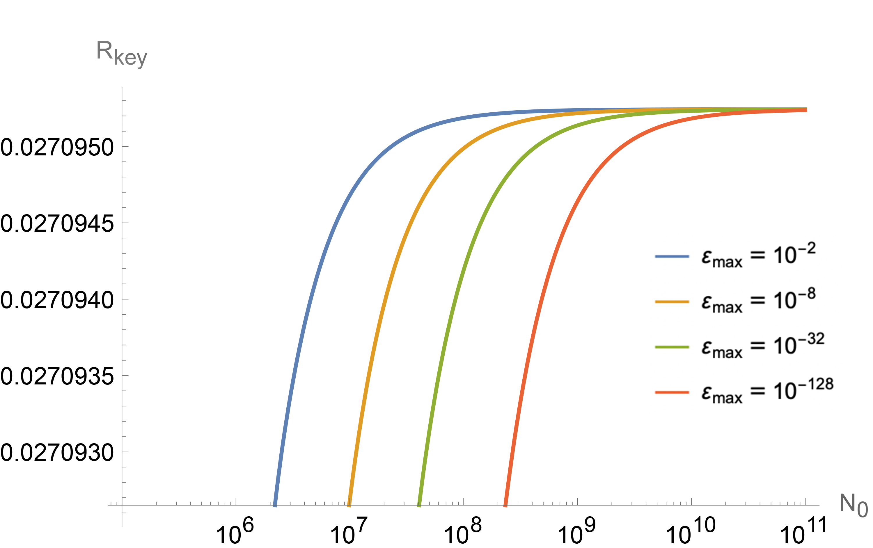
Figure 2: Maximum key rate behaviour as a function of $N_{0}$ for different security levels.

Another important aspect to analyze is the relation between $R_{\textnormal{key}}$ and $N_{0}$, which is shown in Figure 2. Fixing the $\alpha,\delta_{1},\delta_{2},p_{\max}$, there is a clearly marked phase transition-like behaviour in which, for each $\varepsilon_{\max}$, there is a critical value of $N_{0}=N_{\textnormal{crit}}$ before which $R_{\textnormal{key}}=0$, and after which it quickly reaches its maximum value. This result comes from the fact that the parameter estimation requires relatively big sample sizes to reach high confidence. It shows that, even for small $n$, there is a minimum amount of entangled qubits needed to be shared. In some cases, for instance, generating a $1$-bit oblivious key or a $128$-bit one may have similar costs in terms of quantum communication. Because the use of resources of the protocol scales with $N_{0}$, the parameters $\alpha,\delta_{1},\delta_{2}$ should be chosen such that $N_{\textnormal{crit}}$ is the smallest. Figure 3 exemplifies the dependency of $N_{\textnormal{crit}}$ on $\varepsilon_{\max}$.

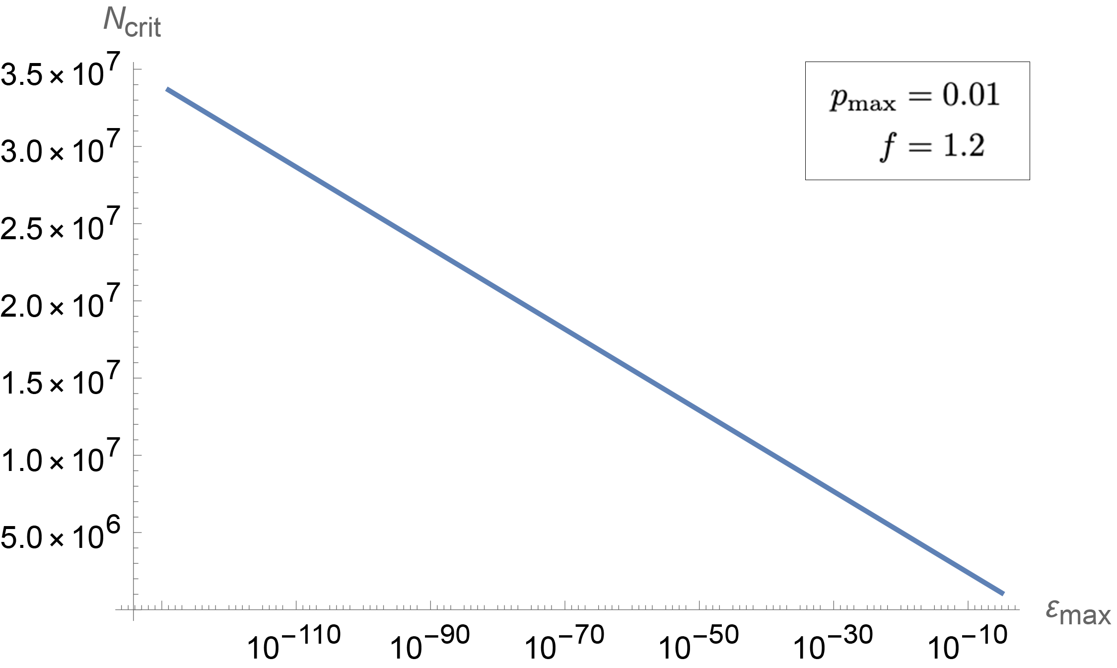
Figure 3: Critical value $N_{\textnormal{crit}}$ of the number of shared qubits needed to obtain positive key rates as a function of the security level. The values of $N_{\textnormal{crit}}$ were computed using the parameters $\alpha,\delta_{1},\delta_{2}$ that minimize the value of $N_{\textnormal{crit}}$ for each $\varepsilon_{\max}$.

3.4 Experimental implementation performance

An experiment was implemented to test the performance of the $\pi_{\textnormal{QROT}}$ protocol with contemporary technology. Data was acquired using a picosecond pulsed photon source in a Sagnac configuration  [45], producing wavelength degenerate, polarization-entangled photons at 1550nm. In this setup, entangled photons were produced via spontaneous parametric down conversion (SPDC) by applying a laser pump beam into a 30mm long periodically-poled potassium titanyl phosphate (ppKTP) crystal. The photon pairs were split using a half-wave plate (HWP) and a polarizing beam splitter (PBS), and then sent to each party where they are detected using superconducting nanowire single-photon detectors.

To test the OT speed of this implementation, different values for the power $P$ of the laser pump were tested, as well as the use of multiplexing. As the $P$ increases, the amount of coincidences detected per second $R_{\textnormal{c}}$ increases, but the fidelity of the produced entangled pairs decreases, resulting in larger values for qubit error rate, which is represented by the protocol parameter $p_{\max}$. The number of maximum potential OT instances per second is computed as

$$R_{OT}=\frac{R_{\textnormal{c}}}{N_{\textnormal{crit}}},$$ (31)

where $N_{\textnormal{crit}}$ is computed using the optimal values of $\alpha,\delta_{1},\delta_{2}$ for the respective error rate $p_{\max}$ associated to $P$, and a given $\varepsilon_{\max}$, assuming perfectly efficient information reconciliation, $f=1$. As seen in Figure 4, for this implementation, the additional coincidence rate gained by increasing $P$ is not enough to compensate for the induced increased error. This result is not immediately obvious, as $N_{\textnormal{crit}}$ does not depend explicitly on $p_{\max}$. The decrease in performance comes from the fact that increasing $p_{\max}$ limits the values that $\delta_{1}$ can have while maintaining positive key rates. This restriction on the values of $\delta_{1}$ ultimately results in an increase in $N_{\textnormal{crit}}$ and therefore, a reduction on $R_{OT}$.

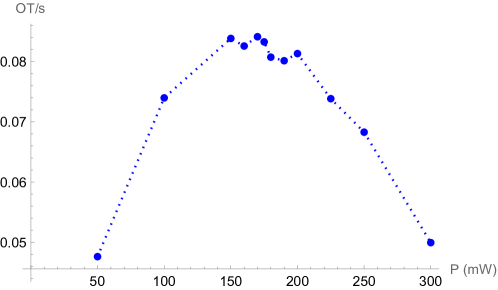
Figure 4: Maximum potential ROT rates as a function of the pump power P for $\varepsilon_{\max}=10^{-8}$. We see that the best performance is obtained at a laser pump power of $P=170$ mW, corresponding to a coincidence rate close to $2.45$ kHz. The uncertainty on the power measurement (x-axis) along with the error bars resulting from the Poissonian noise on the coincidence counts (used to calculate y-values) are negligible with respect to the current plot scale.

Table 1 shows the an example of the performance of the protocol in a real-world implementation using the data from the experimental setup. For the commit/open phase, the weakly-interactive string commitment protocol introduced in [37] was implemented using the BLAKE3 hash function algorithm as a one-way function. For the post-processing phase, a low density parity check (LDPC) code was used for IR, and random binary matrices were used to implement the universal hash family for privacy amplification. We evaluated the performance by the number of $128$-bit ROT instances able to be completed per second.

Parameter	Symbol	Value
Message size (bits)	$n$	$128$
Security level	$\varepsilon_{\textnormal{max}}$	$5.71\text{\times}{10}^{-9}$
Cost in quantum signals	$N_{0}$	$5.86\text{\times}{10}^{6}$
Max allowed QBER	$p_{\textnormal{max}}$	$1.18\%$
Testing set ratio	$\alpha$	$0.35$
Statistical parameter 1	$\delta_{1}$	$9.2\text{\times}{10}^{-3}$
Statistical parameter 2	$\delta_{2}$	$3\text{\times}{10}^{-3}$
IR verifiability security	$\varepsilon_{\textnormal{IR}}$	$2^{-32}$
Commitment binding security	$\varepsilon_{\textnormal{bind}}$	$2^{-32}$
Efficiency of IR	$f$	$1.61$
	ROT rate	$0.023$ ROT/s

Table 1: Table of protocols parameters and the resulting performance. The values of $N_{0}$ and $\delta_{1}$ and the laser pump power were optimized to yield the highest ROT rate for an LDPC code with efficiency f = 1.61.

4 Discussion

Using Naor’s protocol [37] in conjunction with a linear time OWF (such as a hash function fron the SHA3 or BLAKE family), it is possible to implement the required 2-bit commitment in linear time in $k$. On the other hand, using an LDPC code with soft-decision decoding and hash based verification, one can implement an IR scheme which is linear in both the block size $N_{\textnormal{raw}}$ (and therefore $N_{0}$) and $k^{\prime}$. Finally, by taking the universal hash set F to be the set of Toeplitz matrices of size $N_{\textnormal{raw}}\times n$, and using the FFT algorithm for matrix-vector multiplication, the computation of the output strings can be done in time $O(N_{\textnormal{raw}}\log(N_{\textnormal{raw}}))$. Considering that the protocol requires $N_{0}$ commitments and all the remaining computations of random subsets and checks can be done in linear time in $N_{0}$, the total protocol running time is $O(N_{0}(k+k^{\prime}+\log(N_{0}))$.

Regarding the practicality of implementing $\pi_{\textnormal{QROT}}$, the protocol is designed to be compatible with BB84-based QKD setups, both from the physical layer up to the post-processing, only requiring the addition of the commitment scheme. The most important difference to note is that $\pi_{\textnormal{QROT}}$ has significantly lower tolerance for Qubit Error Rate (QBER). While most common QKD protocols can produce keys through QBERs above $10\%$, this protocol is limited to a maximum of $2.8\%$. This comparatively reduces the distances at which the protocol can be successful. However, it is important to note that, as opposed to key distribution between trusting parties, there are legitimate use-cases for OT at short range. While being in proximity to each other can help two trusting parties isolate themselves from a third party eavesdropper, mistrusting parties do not gain anything (security wise) from being in the same place while attempting to do MPC, making the protocol useful regardless of the distance between the users.

Comparisons between classical and quantum protocols can be difficult because physical/technological assumptions, such as access to quantum communication or noisy quantum storage, do not straightforwardly compare with computational hardness assumptions. Furthermore, there is no natural way of quantitatively comparing statistical versus computational security. We can, however, contrast the (dis-)advantages of using a computationally-secure quantum OT protocol as compared to both fully classical computationally-secure protocols, as well as statistically-secure quantum ones.

Classical OT protocols based on asymmetric cryptography comprise the overwhelming majority of current real-world implementations of OT. The obvious main advantage of quantum OT is the weaker computational hardness assumption (OWF vs asymmetric cryptography), while the main advantage of current post-quantum classical OT implementations is speed. As shown in Fig. 4, the presented experimental setup is able to produce up to $~0.08$ OT/s, which pales in comparison to contemporary classical protocols, such as [32, 33, 34, 35], that can achieve upwards of $10^{5}$ OT/s (not including latency between parties) with current off-the-shelf hardware (for more details, see [35]). This difference can be mitigated by the use of OT extension algorithms, as the difference in speed would only matter during the generation of the base OTs. Note that in this case one should use a OT extension that matches the computational assumption of this work, such as [46].

Quantum protocols, both discrete variable (DV) [29] and continuous variable (CV) [31], have been shown to achieve statistically-secure OT in the noisy-storage model. Their experimental implementations show comparable values of quantum communication cost in terms of shared signals: $10^{8}$ (no memory encoding assumption), and $10^{5}$ (Gaussian encoding) for CV, and $10^{7}$ for DV. As shown in Fig. 3, our protocol requires $10^{6}$ quantum signals when matching their security ($\varepsilon=10^{-7}$), which improves upon the alternatives when no additional assumption on the memory encoding of the adversary is made. Less straightforward to compare is the strength of the assumptions of noisy storage and OWFs. We note that the existence of OWFs is an assumption that permeates modern cryptography, from block cipher encryption and message authentication up to public-key cryptography protocols [47], which makes $\pi_{\textnormal{QROT}}$ more suited to be introduced in current cipher suites than protocols with alternative assumptions. In particular, as noted above, OWFs are required for OT extension algorithms.

Regarding potential improvements and further work, we can identify two main directions to build upon this work: performance and security. Regarding performance, we note that dominant term in the expression for $\varepsilon_{max}$ is the one associated with the significance of the parameter estimation (the first term in Eq. 28). This translates into the relatively large values of $N_{0}$ needed to achieve adequate security, which was the bottleneck in the performance of our implementation. One way to reduce the number of signals needed per OT is to modify the protocol to perform many concurrent ROTs in a single run. This would mean performing one single estimation, albeit of a larger sample, that would work for many OTs in such a way that the required number of signals per ROT is decreased. On the topic of increasing security it seems like a natural step to transform our indistinguishability-based security definition into a simulation-based one. This would involve replacing the commitment scheme with one that holds the properties of equivocability and extractability. Such constructions based only on OWF have been developed in [40] and independently in [48]. Although using these type of commitment schemes can non-trivially increase the complexity of the protocol, this type of security is considered to be desirable in the context of using the OTs as a resource for arbitrary MPC.

5 Security Analysis

In this section, we prove the main security result, which relates the overall security of the protocol as a function of its parameters $N_{0},\alpha,\delta_{1}$, and $\delta_{2}$ in Theorem 3.1. For clarity of presentation, we have compacted some of the properties into lemmas, for which detailed proofs can be found in Appendix A.

5.1 Correctness

In order to prove correctness we need to show that either the protocol either finishes with Alice outputting uniformly distributed messages $m_{0},m_{1}$ and Bob outputting a uniformly random bit $c$ and the corresponding message $m_{c}$, or it aborts, except with negligible probability.

Recall that we model the aborted state of the protocol as the zero operator. This way, whenever we have a mixture of states, some of which trigger aborting and some that do not, the abort operation removes the events that trigger it from the mixture, effectively reducing its trace by the probability of aborting. There are three instances where the protocol can abort: first during Step (7) if the estimated qubit error rate is larger than $p_{\max}$; the second one is during Step (9) if Bob does not have enough (mis)matching bases to construct the sets $I_{0},I_{1}$; and finally during Step (11) if the IR verification fails. The probability of aborting in Steps (7) and (11) depends on the particular transformation that the states undergo when being sent from Alice’s to Bob’s laboratory, about which we make no assumptions. We can group these three abort events and denote by $p_{\textnormal{abort}}$ the probability of the protocol aborting by the end of Step (11). The state at this point can be written as $(1-p_{\textnormal{abort}})\rho^{\top}$, where $\rho^{\top}$ represents the normalized state conditioned that the protocol has not aborted by this point. As Lemma 5.1 states, the verifiability property of the Information Reconciliation scheme guarantees that the states that “survive” past Step (11) have the property that Bob’s corrected string $y^{B}$ is the same as Alice’s outcome string $x^{A}_{I_{0}}$, which is uniformly distributed.

Lemma 5.1.

Let $X^{A}_{I_{0}},X^{A}_{I_{1}},C,Y^{B}$ denote the systems holding the information of the respective values $x^{A}_{I_{0}},x^{A}_{I_{1}},c$, and $y^{B}$ of $\pi_{\textnormal{QROT}}$. Denote by $\rho^{\top}$ the parties’ joint state at the end of Step (11) conditioned that Bob constructed the sets $(I_{0},I_{1})$ during Step (9) and the protocol has not aborted. Assume both parties follow the Steps of the protocol, then

$$\rho^{\top}_{X^{A}_{I_{0}},X^{A}_{I_{1}},C,Y^{B}}\approx_{\varepsilon_{\textnormal{IR}}(k^{\prime})}\tilde{\rho}^{\top}_{X^{A}_{I_{0}},X^{A}_{I_{1}},C,Y^{B}},$$ (32)

where $\varepsilon_{\textnormal{IR}}(k^{\prime})$ is a negligible function given by the security of the underlying Information Reconciliation scheme, $k^{\prime}$ its associated security parameter, and

$$\tilde{\rho}^{\top}_{X^{A}_{I_{0}},X^{A}_{I_{1}},C,Y^{B}}=\frac{1}{2^{(2N_{\textnormal{raw}}+1)}}\!\sum_{\begin{subarray}{c}x_{I_{0}},x_{I_{1}}\\ c\end{subarray}}\!|x_{I_{0}}\rangle\ \!\!\!\langle x_{I_{0}}|_{X^{A}_{I_{0}}}|x_{I_{1}}\rangle\ \!\!\!\langle x_{I_{1}}|_{X^{A}_{I_{1}}}|x_{I_{0}}\rangle\ \!\!\!\langle x_{I_{0}}|_{Y^{B}}|c\rangle\ \!\!\!\langle c|_{C}.$$ (33)

During Step (12) universal hashing is used in both $x^{A}_{I_{0}}$ and $x^{A}_{I_{1}}$ to obtain $m_{c}$ and $m_{\bar{c}}$. Because Eq. (33) describes a state for which the $X^{A}_{I_{0}},X^{A}_{I_{1}}$, and $C$ subsystems are independent and uniformly distributed, it follows from Lemma 5.1 that

$$H_{\textnormal{min}}^{\varepsilon_{\textnormal{IR}}(k^{\prime})}(X^{A}_{I_{0}}Y^{B}|X^{A}_{I_{1}}C)_{\rho^{\top}}=H_{\textnormal{min}}^{\varepsilon_{\textnormal{IR}}(k^{\prime})}(X^{A}_{I_{1}}|X^{A}_{I_{0}}Y^{B}C)_{\rho^{\top}}=N_{\textnormal{raw}}.$$ (34)

Finally, using the quantum leftover hash Lemma 2.4 twice (once for $m_{0}$ and $m_{1}$) with the corresponding entropy terms given by Eq. (34), together with Lemma 2.1 (1), we conclude that the state $\rho^{(\textnormal{out})}_{M_{0},M_{1},C,M_{C}}$ of the output systems after the post processing phase satisfies (substituting $p_{\textnormal{succ}}=1-p_{\textnormal{abort}}$)

$$\rho_{M_{0},M_{1},C,M_{C}}^{(\textnormal{out})}\approx_{\varepsilon}\frac{p_{\textnormal{succ}}}{2^{(2n+1)}}\!\!\!\!\!\!\!\!\!\sum\limits_{\begin{subarray}{c}m_{0},m_{1}\in\{0,1\}^{n}\\ c\in\{0,1\}\end{subarray}}\!\!\!\!\!\!\!\!\!|m_{0}\rangle\ \!\!\!\langle m_{0}|_{M_{0}}\otimes|m_{1}\rangle\ \!\!\!\langle m_{1}|_{M_{1}}\otimes|c\rangle\ \!\!\!\langle c|_{C}\otimes|m_{c}\rangle\ \!\!\!\langle m_{c}|_{M_{C}},$$ (35)

with

$$\varepsilon\leq 2^{-\frac{1}{2}(N_{\textnormal{raw}}-n)}+2\varepsilon_{\textnormal{IR}}(k^{\prime}).$$ (36)

5.2 Security against dishonest sender

For this scenario we show that, in the case of an honest Bob and Alice running an arbitrary program, the resulting state after the protocol successfully finishes satisfies Eq. (17). In other words, independently of what quantum state Alice shares at the beginning of the protocol and which operations she performs on her systems, her final state is independent of the value of $c$. We assume that Alice’s laboratory consists of everything outside Bob’s. In particular, this means that she controls the environment, which includes the transmission channels. We also assume that Alice is limited to performing efficient computations.

Let $A$ be the system consisting of all of Alice’s laboratory after Step (1) of the protocol, that is, $A$ contains her part of the shared system and every other ancillary system she may have access, but does not contain any system from Bob’s laboratory, including Bob’s part of the system shared in Step (1). During the execution of the protocol, Alice receives external information from Bob exactly three times: the commitment information shared during Step (4), the opening information $\textnormal{open}_{I_{t}}$ for the commitments associated to the test set $I_{t}$ in Step (6), and the information of the pair of sets $(J_{0},J_{1})=(I_{c},I_{\bar{c}})$ during Step (9). Let $\textnormal{COM}=(\textnormal{COM}_{i})_{i=1}^{N_{0}}$ and $\textnormal{OPEN}=(\textnormal{OPEN}_{i})_{i=1}^{N_{0}}$ be the respective systems used by Bob to store the information of the strings $\textnormal{com}=(\textnormal{com}_{i})_{i=1}^{N_{0}}$ and $\textnormal{open}=(\textnormal{open}_{i})_{i=1}^{N_{0}}$, and let SEP be the system holding the string separation information $(J_{0},J_{1})$. We want to show that, by the end of the protocol, the state of the system $A,\textnormal{COM},\textnormal{OPEN}_{J},\textnormal{SEP},C$ satisfies:

$$\rho_{A,\textnormal{COM},\textnormal{OPEN}_{\bar{I}_{t}},\textnormal{SEP},C}\approx^{(c)}\rho_{A,\textnormal{COM},\textnormal{OPEN}_{\bar{I}_{t}},\textnormal{SEP}}\otimes\mathsf{U}_{C}.$$ (37)

To guarantee that Alice will not be able to obtain information about the value of $c$ during the string separation phase, it is necessary to show that Alice does not have access to the information of Bob’s bases choices $\theta^{B}_{I_{0},I_{1}}$ from the commitments sent by Bob during Step (4) of the protocol. As shown by Lemma 5.2, the shared state of the parties after the commitment information is sent is computationally indistinguishable from a state where Alice’s information is independent of $\theta^{B}_{\bar{I}_{t}}$.

Lemma 5.2.

Assuming Bob follows the protocol, for any $J\subseteq I$, the state of the system $A,\textnormal{COM},\textnormal{OPEN}_{J},\Theta^{B}_{\bar{J}}$ after Step (4) satisfies

$$\rho_{A,\textnormal{COM},\textnormal{OPEN}_{J},\Theta^{B}_{\bar{J}}}\approx^{(c)}\rho_{A,\textnormal{COM},\textnormal{OPEN}_{J}}\otimes\mathsf{U}_{\Theta^{B}_{\bar{J}}}.$$ (38)

At Step (8) of the protocol, Alice sends Bob the system $\Theta^{A}_{\bar{I}_{t}}$ intended to have the information of her measurement bases. Bob then is able to determine the indices for which $\theta^{A}_{\bar{I}_{t}}$ and $\theta^{B}_{\bar{I}_{t}}$ coincide. With this information, he randomly selects sets $I_{0},I_{1}\in\bar{I}_{t}$ of size $N_{\textnormal{raw}}$ for which all indices are associated with matching (for $I_{0}$) or nonmatching (for $I_{1}$) bases. Then he computes $(J_{0},J_{1})=(I_{c},I_{\bar{c}})$, by flipping the order if the pair $(I_{0},I_{1})$ depending on the value of $c$. Clearly, $(J_{0},J_{1})$ depend on both $\theta^{B}_{\bar{I}_{t}}$ and $c$, but as Lemma 5.3 states, any correlation between $(J_{0},J_{1})$, $c$, and Alice’s information disappears if one does not have access to $\theta^{B}_{\bar{I}_{t}}$.

Lemma 5.3.

Denote by $A^{\prime}$ the system representing Alice’s laboratory at the start of Step (9). Let $\mathcal{E}^{(I_{t})}:\mathcal{D}(\mathcal{H}_{A^{\prime},\Theta^{A}_{\bar{I}_{t}},{\Theta^{B}_{\bar{I}_{t}}},C})\rightarrow\mathcal{D}(\mathcal{H}_{A^{\prime},\Theta^{A}_{\bar{I}_{t}},{\Theta^{B}_{\bar{I}_{t}}},C,\textnormal{SEP}})$ be the quantum operation used by Bob to compute the string separation information $(J_{0},J_{1})$ during Step (9) of the protocol. The resulting state after applying $\mathcal{E}^{(I_{t})}$ to a product state of the form

$$\mathcal{E}^{(I_{t})}(\rho_{A^{\prime},\Theta^{A}_{\bar{I}_{t}}}\otimes\mathsf{U}_{\Theta^{B}_{\bar{I}_{t}}}\otimes\mathsf{U}_{C})=\sigma_{A^{\prime},\Theta^{A}_{\bar{I}_{t}},{\Theta^{B}_{\bar{I}_{t}}},C,\textnormal{SEP}},$$ (39)

satisfies:

$$\Tr_{\Theta^{A}_{\bar{I}_{t}},\Theta^{B}_{\bar{I}_{t}}}\big{[}\sigma_{A^{\prime},\Theta^{A}_{\bar{I}_{t}},{\Theta^{B}_{\bar{I}_{t}}},C,\textnormal{SEP}}\big{]}=\sigma_{A^{\prime}}\otimes\sigma_{\textnormal{SEP}}\otimes\mathsf{U}_{C}.$$ (40)

A proof of both Lemmas 5.2 and 5.3 can be found in Appendix A.3. By setting $J=I_{t}$, Lemma 5.2 guarantees that Alice’s system’s state after the opening information has been sent is computationally indistinguishable from one that is completely uncorrelated with Bob’s measurement basis information in $\bar{I}_{t}$. Additionally, by recalling that the value of $c$ is sampled independently of any of the considered systems, we know that the state $\rho_{{A^{\prime},\Theta^{A}_{\bar{I}_{t}},\Theta^{B}_{\bar{I}_{t}}},C}$ before $(J_{0},J_{1})$ is computed has the required product form and, from Lemma 5.3, we conclude that the state of all of Alice’s system at this point is computationally indistinguishable from a state uncorrelated with $C$. Let $\mathcal{E}$ be the operation Alice performs in her system from here to the end the protocol. By using Lemma 2.2 (4) and grouping all of Alice’s systems into $S$, we obtain the desired result:

$$\rho_{S,C}\approx^{(c)}\rho_{S}\otimes\mathsf{U}_{C}.$$ (41)

5.3 Security against dishonest receiver

We consider now the scenario in which Alice runs the protocol honestly and Bob runs an arbitrary program. We want to show that the state after finishing the protocol successfully satisfies Eq. (18). This means that the state at the end of the protocol can be described as a mixture of states where Bob’s system is uncorrelated with at least one of the two strings outputted by Alice. Similarly to the dishonest sender’s case, we assume that Bob’s laboratory consists of everything outside Alice’s, which means that he controls the communication channels and the environment. However, we do not assume that Bob is restricted to efficient computations.

The values of Alice’s output strings depend on several quantities: Alice’s measurement outcomes, the choice of the $I_{t},J_{0},J_{1}$ subsets, and the choice of hashing function $f$ during the post-processing phase of the protocol. From all of these, the only ones that are not made explicitly public during the protocol’s execution are Alice’s measurement outcomes. Instead, partial information of these outcomes is revealed at different steps of the protocol. Let $x^{A}_{J_{0}},x^{A}_{J_{1}}$ be the sub-strings of measurement outcomes used to compute Alice’s outputs $m_{0},m_{1}$, respectively, and let $R$ denote Bob’s system at the end of the protocol (which includes all the systems that Alice sent during the execution of the protocol). In order to prove security we need to show that the joint state of the system $X^{A}_{J_{0}},X^{A}_{J_{1}},R$ can be written as a mixture of states $\rho^{b}$ (with $b\in\{0,1\}$) such that the conditional min-entropy $H_{\textnormal{min}}^{\varepsilon}(X^{A}_{J_{b}}|R)_{\rho^{b}}$ is high enough, so that we can use the leftover hash Lemma 2.4 to guarantee that the outcome of the universal hashing $m_{b}=f(x^{A}_{J_{b}})$ is uncorrelated with $R$.

At the start of the protocol the parties share a completely correlated entangled system. If the parties make measurements as intended, their outcomes will be only partially correlated, but if Bob was able to postpone his measurement until after Alice’s reveals her measurement bases, Bob could potentially obtain the whole information of $x^{A}$ by measuring in the appropriate basis on his system. To prevent this, Bob is required to commit his measurement bases and results to Alice before knowing which set is going to be tested. Then a statistical test is performed in Step (7) to estimate the correlation of Alice’s measurement outcomes with with the ones that Bob committed. As Lemma 5.4 states, any state passing the aforementioned test is such that, regardless of how Bob defines the sets $(J_{0},J_{1})$ during the string separation phase, there is a minimum of uncertainty that he has with respect to Alice’s measurement outcomes. Recall that, when Alice is honest, the overall state of the protocol before Step (8) will be a partially classical state, which could be written as a mixture over all of Alice’s classical information. Let $\vec{\tau}=(x^{A}_{I_{t}},\theta^{A},r,\textnormal{com},I_{t},I_{s},\textnormal{open}_{I_{t}})$ denote the transcript of the protocol up to Step (8), and let $\rho_{X^{A}B}(\vec{\tau},J_{0},J_{1})$ be the joint state of Alice’s measurement outcomes and Bob’s laboratory conditioned to $\vec{\tau},J_{0},J_{1}$.

Lemma 5.4.

Assuming Alice follows the protocol, let $T,\textnormal{SEP},B$ denote the systems of the protocols transcript, the strings $J_{0},J_{1}$, and Bob’s laboratory at the end of Step (9) of the protocol, and let $\rho_{T,\textnormal{SEP},X^{A},B}$ be the state of the joint system at that point. There exists a state $\tilde{\rho}_{T,\textnormal{SEP},X^{A},B}$, which is classical in $T$ and SEP such as:

1. The conditioned states $\tilde{\rho}_{X^{A},B}(\vec{\tau},J_{0},J_{1})$ satisfy:

   $$H_{\textnormal{min}}(X^{A}_{J_{0}}|X^{A}_{J_{1}}B)_{\tilde{\rho}(\vec{\tau},J_{0},J_{1})}+H_{\textnormal{min}}(X^{A}_{J_{1}}|X^{A}_{J_{0}}B)_{\tilde{\rho}(\vec{\tau},J_{0},J_{1})}\geq 2N_{\text{raw}}\left(\frac{1}{2}-\delta_{2}-h\left(\frac{p_{\text{max}}+\delta_{1}}{\frac{1}{2}-\delta_{2}}\right)\right),$$ (42)

2. $\rho_{T,\textnormal{SEP},X^{A},B}\approx_{\varepsilon}\tilde{\rho}_{T,\textnormal{SEP},X^{A},B}$, with

   $$\varepsilon=\left(2(e^{-\frac{1}{2}\alpha(1-\alpha)^{2}N_{0}\delta^{2}_{1}}+e^{-\frac{1}{2}(\frac{1}{2}-\delta_{2})\alpha N_{0}\delta^{2}_{1}})\right)^{\frac{1}{2}}+e^{-D_{KL}(\frac{1}{2}-\delta_{2}|\frac{1}{2})(1-\alpha)N_{0}}+\varepsilon_{\textnormal{bind}}(k),$$ (43)

   where $h(\cdot)$ and $D_{KL}(\cdot|\cdot)$ denote the binary entropy and the binary relative entropy functions, respectively, and $\varepsilon_{\textnormal{bind}}(k)$ is a negligible function given by the binding property of the commitment scheme.

To reach the desired result, we will first show that a state $\tilde{\rho}_{T,\textnormal{SEP},X^{A},B}$ satisfying Lemma 5.4 (1) also satisfies a tighter version Lemma 3.2, and then use Lemma 5.4 (2) to attain the bound for the real protocol’s outcome. Since $\tilde{\rho}_{T,\textnormal{SEP},X^{A},B}$ is classical in both $T$ and SEP we can write the state of the joint system of Alice’s measurement outcomes and Bob’s laboratory as a mixture over all the possible transcripts at that point, that is:

$$\tilde{\rho}_{X^{A}B}=\sum_{\begin{subarray}{c}\vec{\tau}\\ {J_{0},J_{1}}\end{subarray}}P(\vec{\tau},J_{0},J_{1})\tilde{\rho}_{X^{A}B}(\vec{\tau},J_{0},J_{1}),$$ (44)

where $P(\vec{\tau},J_{0},J_{1})$ defines a probability distribution which is dependent on Bob’s behavior during the previous steps. We can now separate the $\rho_{X^{A}B}(\vec{\tau},J_{0},J_{1})$ in two categories depending on which of the $x^{A}_{J_{0}},x^{A}_{J_{1}}$ is the least correlated with Bob’s system. Consider the function $b(\vec{\tau},J_{0},J_{1})$ to be equal to $0$ if $H_{\textnormal{min}}^{\varepsilon}(X^{A}_{J_{0}}|X^{A}_{J_{1}}B)_{\rho(\vec{\tau},J_{0},J_{1})}\geq H_{\textnormal{min}}^{\varepsilon}(X^{A}_{J_{1}}|X^{A}_{J_{0}}B)_{\rho(\vec{\tau},J_{0},J_{1})}$, and equal to $1$ otherwise. By regrouping the terms from (44) for which the value of $b$ is the same, we can rewrite the joint state as:

$$\tilde{\rho}_{X^{A}B}=\sum_{b\in\{0,1\}}P_{b}\tilde{\rho}^{b}_{X^{A}B}.$$ (45)

where, from Lemma 5.4 and recalling that, as Lemma 2.3 (5) states, the min-entropy of a mixture is lower bounded by that of the term with the least min-entropy, we know that

$$H_{\textnormal{min}}(X^{A}_{J_{b}}|X^{A}_{J_{\bar{b}}}B)_{\tilde{\rho}^{b}}\geq N_{\text{raw}}\left(\frac{1}{2}-\delta_{2}-h\left(\frac{p_{\text{max}}+\delta_{1}}{\frac{1}{2}-\delta_{2}}\right)\right).$$ (46)

At Step (10), Alice shares with Bob the syndromes $S_{0}=\mathtt{syn}(x^{A}_{J_{0}})$ and $S_{1}=\mathtt{syn}(x^{A}_{J_{1}})$. Since these syndromes are completely determined by the respective sub-strings $x^{A}_{J_{i}}$, we know that

$$H_{\textnormal{min}}(X^{A}_{J_{b}}|S_{b}S_{\bar{b}}B) \geq H_{\textnormal{min}}(X^{A}_{J_{b}}|S_{b}X^{A}_{J_{\bar{b}}}B)$$

$$\geq H_{\textnormal{min}}(X^{A}_{J_{b}}|X^{A}_{J_{\bar{b}}}B)-H_{\max}(S_{b})$$

$$\geq N_{\text{raw}}\left(\frac{1}{2}-\delta_{2}-h\left(\frac{p_{\text{max}}+\delta_{1}}{\frac{1}{2}-\delta_{2}}\right)-f\cdot h(p_{\text{max}}+\delta_{1})\right),$$ (47)

where the second inequality follows from Lemma 2.3 (3) and (4), and the max entropy term $H_{\max}(S_{b})$ is upper bounded by the size in bits of the syndrome $\ell=N_{\text{raw}}(f\cdot h(p_{\text{max}}+\delta_{1}))$. Now we can apply Equation (5.3) to Lemma 2.4, which states that, for the outcomes $M_{0},M_{1}$ of the universal hashing by Alice in Step (12) and the Bob’s final system $R$ it holds that

$$\tilde{\rho}_{R,M_{0},M_{1}}^{b}\approx_{\varepsilon^{\prime}}\tilde{\rho}_{R,M_{\bar{b}}}^{b}\otimes\mathsf{U}_{M_{b}},$$ (48)

with

$$\varepsilon^{\prime}=\frac{1}{2}\cdot 2^{n-N_{\text{raw}}\left(\frac{1}{2}-\delta_{2}-h\left(\frac{p_{\text{max}}+\delta_{1}}{\frac{1}{2}-\delta_{2}}\right)-f\cdot h(p_{\text{max}}+\delta_{1})\right)}.$$ (49)

where $\varepsilon$ is given by Eq. (43). Finally, by applying Lemma 2.1 (3) and (4) to Equations (45) and  (48), and then Lemma 2.1 (1) to Eq. (43) we get the desired result:

$$\rho_{R,M_{0},M_{1}}\approx_{\varepsilon}\sum_{b}P_{b}\,\rho_{R,M_{\bar{b}}}^{b}\otimes\mathsf{U}_{M_{b}},$$ (50)

with

$$\varepsilon =\sqrt{2}\left(e^{-\frac{1}{2}(1-\alpha)^{2}N_{\textnormal{test}}\delta^{2}_{1}}+e^{-\frac{1}{2}N_{\textnormal{check}}\delta^{2}_{1}}\right)^{\frac{1}{2}}+e^{-D_{KL}(\frac{1}{2}-\delta_{2}|\frac{1}{2})(1-\alpha)N_{0}}+\varepsilon_{\textnormal{bind}}(k)$$ (51)

$$\quad\quad+\frac{1}{2}\cdot 2^{n-N_{\textnormal{raw}}\left(\frac{1}{2}-\delta_{2}-h\left(\frac{p_{\textnormal{max}}+\delta_{1}}{\frac{1}{2}-\delta_{2}}\right)-f\cdot h(p_{\textnormal{max}}+\delta_{1})\right)}.$$

6 Experimental Implementation

6.1 Description of the Setup

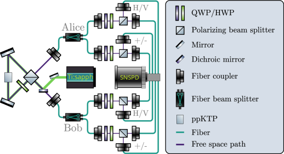
Figure 5: Experimental setup. Polarization-entangled photon pairs are created using spontaneous parametric down conversion. Alice’s and Bob’s photons are individually fiber coupled and each sent to 50/50 fiber beam splitters, which probabilistically route them to free-space polarization projection stages - one projecting onto the linear, and one onto the diagonal basis each for Bob and Alice.

A schematic representation of the experimental setup can be seen in Fig. 5. Spontaneous parametric down conversion (SPDC), attributed to Alice, is used to create polarization entangled photon pairs in the state ${|{\Psi^{+}}\rangle}=\frac{1}{\sqrt{2}}\left({|{HH}\rangle}+{|{VV}\rangle}\right)$, which are coupled into optical fiber. One photon is sent through a 50/50 fiber beam splitter, probabilistically routing it to one of two polarization projection stages. There, a quarter-wave plate (QWP), a half-wave plate (HWP) and a polarizing beam splitter (PBS) are used to project the photons state onto the linear ($H/V$) or diagonal ($+/-$) basis, respectively. All photons are sent to superconducting nanowire single photon detectors (SNSPDs) and their arrival time is recorded using a time tagging module (TTM). The second photon of the state ${|{\Psi^{+}}\rangle}$, attributed to Bob, travels through an equivalent probabilistic projection setup.

Entangled photon pairs are generated using collinear type-II SPDC in a periodically poled $\mathrm{KTiOPO_{4}}$-crystal with a poling period of $46.2\text{\,}\mathrm{\SIUnitSymbolMicro m}$ inside of a sagnac interferometer. The pump light is produced by a pulsed Ti:Sapphire laser (Coherent Mira 900HP) with a pulse width of $2.93\text{\,}\mathrm{ps}$ and a central wavelength of $\lambda_{p}=$773\text{\,}\mathrm{nm}$$, creating degenerate single-photon pairs at $\lambda_{s}=\lambda_{i}=$1546\text{\,}\mathrm{nm}$$. The laser’s inherent pulse repetition rate of $76\text{\,}\mathrm{MHz}$ is doubled twice to $304\text{\,}\mathrm{MHz}$ using a passive temporal multiplexing scheme [49]. About $100\text{\,}\mathrm{m}$ of single mode fiber separate the experimental setup from the $1\text{\,}\mathrm{K}$ cryostat housing the SNSPDs with a detection efficiency of around $95\text{\,}\mathrm{\char 37\relax}$ and a dark-count rate of around $300\text{\,}\mathrm{Hz}$.

6.2 Practical security

Any photonic implementation of quantum cryptography presents experimental imperfections, which can be exploited by dishonest parties to enhance their cheating probability and violate ideal security assumptions. Important examples of such imperfections include multiphoton noise, lossy/noisy quantum channels, non-unit detection efficiency and detector dark counts.

Dishonest sender. In our experiment, threshold detectors cannot resolve the incident photon number, and unexpected click patterns can occur. For example, several of the four detectors may simultaneously click for a given round, which leads to an inconclusive measurement outcome that has to be reported by the honest receiver. This in turn allows a dishonest sender to gain significant information about the receiver’s measurement basis by sending polarized multiphoton states, except when the following reporting strategy is used [50]:

• $1$ click: assign the correct bit value and report a successful round

• $2$ clicks from the same basis: assign a random bit value and report a successful round

• any other click pattern: report an unsuccessful round

Dishonest receiver. Due to Poisson statistics in the SPDC process, emission of double pairs can occur for a given round. When the two photons kept by the sender are projected onto the same state (i.e. only a single click is recorded in the four detectors), the two photons sent to Bob have the same polarization. In this case, a dishonest receiver can split the two photons and measure one in each basis. The probability of such multiphoton states occurring is characterized and bounded by our second-order correlation measurement.

7 Acknowledgements

M.L., P.M., and N.P. acknowledge Fundação para a Ciência e Tecnologia (FCT), Instituto de Telecomunicações Research Unit, ref. UIDB/50008/2020, UIDP/50008/2020 and PEst-OE/EEI/LA0008/2013, as well as FCT projects QuantumPrime reference PTDC/EEI-TEL/8017/2020. M.L. acknowledges PhD scholarship PD/BD/114334/2016. N.P. acknowledges the FCT Estímulo ao Emprego Científico grant no. CEECIND/04594/2017/CP1393/CT000. P.S., M.B. and P.W. acknowledge funding from the European Union’s Horizon Europe research and innovation program under Grant Agreement No. 101114043 (QSNP), along with the Austrian Science Fund FWF 42 through [F7113] (BeyondC) and the AFOSR via FA9550-21-1-0355 (QTRUST). D.E. was supported by the JST Moonshot R&D program under Grant JPMJMS226C.

Appendix A Detailed proof of Theorem 3.1

A.1 Supporting lemmas

One of the main features to analyze for the security against a dishonest receiver is the potential information that he can learn about the the sender’s strings given the quantum state that remains with him after the commit/open phase. In order to talk about the security of the protocol independently of the specific cheating strategy that may be used by the dishonest parties (or possible effects that the environment can have in the shared quantum state), we want to understand the properties that a quantum state that passes Alice’s test at Step (7) can have. We do this through the following lemma, a version of which was originally proven in [22]. Here, we provide a more self contained statement and make explicit the trace distance bound.

Lemma A.1.

Let $\varepsilon>0$, $I=\{1,\ldots,N\}$, and $\rho_{T,\hat{X},X,E}$ be a density operator of the form

$$\begin{split}\rho_{T,\hat{X},X,E}&=\!\!\!\!\!\sum_{\begin{subarray}{c}I_{1},I_{2}\\ \in\mathcal{P}(I)\setminus\{\emptyset\}\end{subarray}}\!\!\!\!\!q(I_{1},I_{2})|I_{1},I_{2}\rangle\ \!\!\!\langle I_{1},I_{2}|_{T}\otimes|\hat{x}\rangle\ \!\!\!\langle\hat{x}|_{\hat{X}}\otimes|\psi\rangle\ \!\!\!\langle\psi|_{X,E}\\ {|{\psi}\rangle}_{X,E}&=\sum_{x\in\{0,1\}^{N}}\beta^{x}{|{x}\rangle}_{X}{|{\phi^{x}}\rangle}_{E},\end{split}$$ (52)

where $\dim(\mathcal{H}_{\hat{X}})=\dim(\mathcal{H}_{X})=2^{N}$ and $\mathcal{P}(I)$ denotes the set of all subsets of $I$. For each $I_{1},I_{2}$ define the set

$$B_{I_{1},I_{2}}=\{x\in\{0,1\}^{N}:|r_{\textnormal{H}}(x_{I_{1}}\oplus\hat{x}_{I_{1}})-r_{\textnormal{H}}(x_{I_{2}}\oplus\hat{x}_{I_{2}})|<\varepsilon\}.$$ (53)

Additionally, let $\mathcal{Q}(N,\varepsilon)$ be a function such that, whenever the subsets $I_{1},I_{2}$ are sampled according to $q$, it holds that

$$\Pr[|r_{\textnormal{H}}(x_{I_{1}}\oplus\hat{x}_{I_{1}})-r_{\textnormal{H}}((x_{I_{2}}\oplus\hat{x}_{I_{2}})|>\varepsilon]\leq\mathcal{Q}(N,\varepsilon)$$ (54)

independently of $x$. There exists a state $\tilde{\rho}_{T,\hat{X},X,E}$ of the form

$$\begin{split}\tilde{\rho}_{T,\hat{X},X,E}&=\!\!\!\!\!\sum_{\begin{subarray}{c}I_{1},I_{2}\\ \in\mathcal{P}(I)\setminus\{\emptyset\}\end{subarray}}\!\!\!\!\!q(I_{1},I_{2})|I_{1},I_{2}\rangle\ \!\!\!\langle I_{1},I_{2}|_{T}\otimes|\hat{x}\rangle\ \!\!\!\langle\hat{x}|_{\hat{X}}\otimes|\psi_{I_{1},I_{2}}\rangle\ \!\!\!\langle\psi_{I_{1},I_{2}}|_{X,E}\\ {|{\psi_{I_{1},I_{2}}}\rangle}&=\sum_{x\in B_{I_{1},I_{2}}}\tilde{\beta}^{x}_{I_{1},I_{2}}{|{x}\rangle}_{X}{|{\phi^{x}_{I_{1},I_{2}}}\rangle}_{E}\end{split}$$ (55)

such that

$$D(\rho_{T,\hat{X},X,E},\tilde{\rho}_{T,\hat{X},X,E})\leq\mathcal{Q}(N,\varepsilon)^{\frac{1}{2}}.$$ (56)

Proof.

First, we choose an adequate definition for the $\tilde{\beta}^{x}_{I_{1},I_{2}}$ and then show that, under that choice, the bound in Eq. (56) holds. Note that we can write the state

$$\begin{split}{|{\psi}\rangle}_{X,E}&=\sum_{x\in\{0,1\}^{N}}\beta_{x}{|{x}\rangle}_{X}{|{\phi^{x}}\rangle}_{E}\\ &=\underbrace{\left(\sum_{x\in B_{I_{1},I_{2}}}|\beta_{x}|^{2}\right)^{\frac{1}{2}}}_{\lambda_{I_{1},I_{2}}}\underbrace{\frac{\sum_{x\in B_{I_{1},I_{2}}}\beta_{x}{|{x}\rangle}_{X}{|{\phi^{x}}\rangle}_{E}}{\left(\sum_{x\in B_{I_{1},I_{2}}}|\beta_{x}|^{2}\right)^{\frac{1}{2}}}}_{{|{\psi_{I_{1},I_{2}}}\rangle}_{X,E}}+\underbrace{\left(\sum_{x\notin B_{I_{1},I_{2}}}|\beta_{x}|^{2}\right)^{\frac{1}{2}}}_{\lambda^{\perp}_{I_{1},I_{2}}}\underbrace{\frac{\sum_{x\notin B_{I_{1},I_{2}}}\beta_{x}{|{x}\rangle}_{X}{|{\phi^{x}}\rangle}_{E}}{\left(\sum_{x\notin B_{I_{1},I_{2}}}|\beta_{x}|^{2}\right)^{\frac{1}{2}}}}_{{|{\psi^{\perp}_{I_{1},I_{2}}}\rangle}_{X,E}}\end{split}$$ (57)

The trace distance between the pure states ${|{\psi}\rangle}$ and ${|{\psi_{I_{1},I_{2}}}\rangle}$ is given by $\sqrt{1-|\langle\psi|\psi_{I_{1},I_{2}}\rangle|^{2}}=\lambda^{\perp}_{I_{1},I_{2}}$, hence the trace distance between the complete joint states is given by

$$\begin{split}D(\rho_{T,\hat{X},X,E},\tilde{\rho}_{T,\hat{X},X,E})^{2}&\leq\ \left(\sum_{I_{1},I_{2}\in\mathcal{T}(N,\alpha)}qD(|\psi\rangle\ \!\!\!\langle\psi|_{X,E},|\psi_{I_{1},I_{2}}\rangle\ \!\!\!\langle\psi_{I_{1},I_{2}}|_{X,E})\right)^{2}\\ &=\left(\sum_{I_{1},I_{2}\in\mathcal{T}(N,\alpha)}q\lambda^{\perp}_{I_{1},I_{2}}\right)^{2}\\ &\leq\sum_{I_{1},I_{2}\in\mathcal{T}(N,\alpha)}q{\lambda^{\perp}_{I_{1},I_{2}}}^{2},\end{split}$$ (58)

where the Jensen’s inequality was used in the last Step. We proceed now to bound the right side of Eq. (58). For that purpose consider the function:

$$\xi(I_{1},I_{2},x)=\begin{cases}0&\quad\text{if}\quad x\in B_{I_{1},I_{2}}\\ 1&\quad\text{otherwise}\end{cases},$$ (59)

so that

$$\begin{split}\sum_{I_{1},I_{2}}q(I_{1},I_{2})\xi(I_{1},I_{2},x)=\Pr[|r_{\textnormal{H}}(\hat{x}\oplus x|_{I_{1}})-r_{\textnormal{H}}(\hat{x}\oplus x|_{I_{2}})|>\varepsilon]=\mathcal{Q}(N,\varepsilon)\end{split}$$ (60)

hence,

$$\begin{split}||\rho_{T,\hat{X},X,E}-\tilde{\rho}_{T,\hat{X},X,E}||^{2}&\leq\sum_{I_{1},I_{2}}q(I_{1},I_{2}){\lambda^{\perp}_{I_{1},I_{2}}}^{2}\\ &=\sum_{I_{1},I_{2}}q(I_{1},I_{2})\sum_{x\notin B_{I_{1},I_{2}}}|\beta_{x}|^{2}\\ &=\sum_{I_{1},I_{2}}q(I_{1},I_{2})\sum_{x\in\{0,1\}^{N}}\xi(I_{1},I_{2},x)|\beta_{x}|^{2}\\ &=\sum_{x\in\{0,1\}^{N}}|\beta_{x}|^{2}\sum_{I_{1},I_{2}}q(I_{1},I_{2})\xi(I,x)\\ &\leq\sum_{x\in\{0,1\}^{N}}|\beta_{x}|^{2}\mathcal{Q}(N,\varepsilon)=\mathcal{Q}(N,\varepsilon),\end{split}$$ (61)

as required. ∎

In order to use the above result in the context of the $\pi_{\textnormal{QROT}}$ protocol, we need to find an appropriate function $\mathcal{Q}(N,\varepsilon)$ that satisfies Eq. (54) for the case when the $\hat{x},x$ are the respective measurement outcomes of Alice and Bob when measuring in the same basis. We do this through the following lemma based on the Hoeffding inequality for sampling without replacement.

Definition A.1.

Given a set $I$ and an integer $n\leq|I|$, define the set $\mathcal{T}(n,I)$ as the set of all subsets of $I$ with size $n$.

Lemma A.2.

(Hoeffding’s inequalities)
Let $x\in\{0,1\}^{N}$, $\delta>0$, $I=\{1,\ldots,N\}$ and $0<\alpha<\frac{1}{2}$ such that $\alpha N\in\mathbb{N}$.

1. (Inequality for sampling without replacement comparing the sampled subset with the whole set) For $I_{t}\in\mathcal{T}(\alpha N,I)$ sampled uniformly, it holds that

   $$\Pr[|r_{\textnormal{H}}(x|_{I_{t}})-r_{\textnormal{H}}(x)|>\delta]\leq 2e^{-2\alpha N\delta^{2}}.$$ (62)

2. (Inequality for sampling without replacement comparing the sampled subset with its complement)

   $$\Pr[|r_{\textnormal{H}}(x|_{I_{t}})-r_{\textnormal{H}}(x|_{\bar{I}_{t}})|>\delta]\leq 2e^{-2\alpha(1-\alpha)^{2}N\delta^{2}}.$$ (63)

3. (Inequality for sampling without replacement comparing the sampled subset with its complement and ignoring part of the sample) Let $n\in\{n_{0},\ldots,\alpha N\}$ be sampled according to some distribution $P(n)$. For $I_{s}\in\mathcal{T}(n,I_{t})$ sampled uniformly, it holds that

   $$\Pr[|r_{\textnormal{H}}(x|_{I_{s}})-r_{\textnormal{H}}(x|_{\bar{I}_{t}})|>\delta]\leq 2(e^{-\frac{1}{2}\alpha(1-\alpha)^{2}N\delta^{2}}+e^{-\frac{1}{2}n_{0}\delta^{2}}).$$ (64)

Proof.

1. This is the original Hoeffding inequality for sampling without replacement, the proof of which can be found in [51].

2. Note that we can write $r_{\textnormal{H}}(x)=\alpha r_{\textnormal{H}}(x|_{I_{t}})+(1-\alpha)r_{\textnormal{H}}(x|_{\bar{I}_{t}})$. Substituting $r_{\textnormal{H}}(x)$ in (62) we get

   $$\Pr[|r_{\textnormal{H}}(x|_{I_{t}})-\alpha r_{\textnormal{H}}(x|_{I_{t}})+(1-\alpha)r_{\textnormal{H}}(x|_{\bar{I}_{t}})|>\delta^{\prime}] =\Pr[|r_{\textnormal{H}}(x|_{I_{t}})-r_{\textnormal{H}}(x|_{\bar{I}_{t}})|>\delta^{\prime}/(1-\alpha)]$$ (65)

   $$\leq 2e^{-2\alpha N\delta^{\prime 2}}.$$ (66)

   The result is obtained by taking $\delta^{\prime}=(1-\alpha)\delta$

3. Let us consider first the case where $n$ is fixed. From the triangle inequality we know that

   $$|r_{\textnormal{H}}(x|_{I_{s(n)}})-r_{\textnormal{H}}(x|_{\bar{I}_{t}})|>\delta \Rightarrow|r_{\textnormal{H}}(x|_{I_{s(n)}})-r_{\textnormal{H}}(x|_{I_{t}})|+|r_{\textnormal{H}}(x|_{I_{t}})-r_{\textnormal{H}}(x|_{\bar{I}_{t}})|>\delta$$ (67)

   $$\Rightarrow|r_{\textnormal{H}}(x|_{I_{s(n)}})-r_{\textnormal{H}}(x|_{I_{t}})|>\delta/2\vee|r_{\textnormal{H}}(x|_{I_{t}})-r_{\textnormal{H}}(x|_{\bar{I}_{t}})|>\delta/2,$$ (68)

   and hence, by the union bound

   $$\Pr[|r_{\textnormal{H}}(x|_{I_{s(n)}})-r_{\textnormal{H}}(x|_{\bar{I}_{t}})|>\delta] \leq\Pr[|r_{\textnormal{H}}(x|_{I_{s(n)}})-r_{\textnormal{H}}(x|_{I_{t}})|+|r_{\textnormal{H}}(x|_{I_{t}})-r_{\textnormal{H}}(x|_{\bar{I}_{t}})|>\delta]$$ (69)

   $$\leq\Pr[|r_{\textnormal{H}}(x|_{I_{s(n)}})-r_{\textnormal{H}}(x|_{I_{t}})|>\delta/2]$$

   $$\quad\quad\quad+\Pr[|r_{\textnormal{H}}(x|_{I_{t}})-r_{\textnormal{H}}(x|_{\bar{I}_{t}})|>\delta/2]$$ (70)

   $$\leq 2e^{-\frac{1}{2}n\delta^{2}}+2e^{-\frac{1}{2}\alpha(1-\alpha)^{2}N\delta^{2}},$$ (71)

   where the last expression comes from applying the (b) and (a) inequalities to the first and second terms of (70) respectively. Using this, we can consider the case in which $n$ is not fixed, but instead follows a probability distribution $P(n)$ such that $P(n)=0$ for $n<n_{0}$. For this case

   $$\Pr[|r_{\textnormal{H}}(x|_{I_{s}})-r_{\textnormal{H}}(x|_{\bar{I}_{t}})|>\delta] =\sum_{n}P(n)\Pr[|r_{\textnormal{H}}(x|_{I_{s(n)}})-r_{\textnormal{H}}(x|_{\bar{I}_{t}})|>\delta]$$ (72)

   $$\leq\sum_{n}P(n)2(e^{-\frac{1}{2}\alpha(1-\alpha)^{2}N\delta^{2}}+e^{-\frac{1}{2}n\delta^{2}})$$ (73)

   $$\leq 2\sum_{n}P(n)(e^{-\frac{1}{2}\alpha(1-\alpha)^{2}N\delta^{2}}+e^{-\frac{1}{2}n_{0}\delta^{2}})$$ (74)

   $$=2(e^{-\frac{1}{2}\alpha(1-\alpha)^{2}N\delta^{2}}+e^{-\frac{1}{2}n_{0}\delta^{2}}).$$ (75)

∎

The following lemma helps us bound the conditional min-entropy of a partially measured pure state by comparing it with the one of an appropriately chosen, partially measured mixed state. A proof of this result can be found in [52].

Lemma A.3.

(Entropy bound for post-measurement states)
Let $\mathcal{H}_{A}$ and $\mathcal{H}_{E}$ be Hilbert spaces and $\{{|{x}\rangle}\}_{x\in\mathcal{X}},\{{|{y}\rangle}\}_{y\in\mathcal{Y}}$ be orthonormal bases for $\mathcal{H}_{A}$. Let $J\subseteq\mathcal{X}$, define the states

$$\rho_{AE}=|\phi\rangle\ \!\!\!\langle\phi|_{AE}\;\;\;\;\textit{with}\;\;\;\;{|{\phi}\rangle}_{AE}=\sum_{x\in J}\beta_{x}{|{x}\rangle}_{A}{|{\phi^{x}}\rangle}_{E},$$ (76)

$$\rho^{\textnormal{mix}}_{AE}=\sum_{x\in J}{|\beta_{x}|^{2}}|x\rangle\ \!\!\!\langle x|_{A}\otimes|\phi^{x}\rangle\ \!\!\!\langle\phi^{x}|_{E}.$$ (77)

Denote by $\sigma_{YE}$ and $\sigma^{\textnormal{mix}}_{YE}$ the states resulting from measuring the subsystem $A$ of $\rho_{AE}$ and $\rho^{\textnormal{mix}}_{AE}$ respectively in the basis $\{{|{y}\rangle}\}_{y\in\mathcal{Y}}$, storing the result in the system $Y$, and then tracing out the $A$ subsystem; then it holds that

$$H_{\textnormal{min}}(Y|E)_{\sigma}\geq H_{\textnormal{min}}(Y|E)_{\sigma^{\textnormal{mix}}}-\log|J|.$$ (78)

A.2 Proof of Lemma 5.1

Here we present a proof of Lemma 5.1 used in the protocol’s correctness analysis in Section 5.

Lemma A.4.

Let $X^{A}_{I_{0}},X^{A}_{I_{1}},C,Y^{B}$ denote the systems holding the information of the respective values $x^{A}_{I_{0}},x^{A}_{I_{1}},c$, and $y^{B}$ of $\pi_{\textnormal{QROT}}$. Denote by $\rho^{\top}$ the parties’ joint state at the end of Step (11) conditioned that Bob constructed the sets $(I_{0},I_{1})$ during Step (9) and the protocol has not aborted. Assume both parties follow the steps of the protocol, then

$$\rho^{\top}_{X^{A}_{I_{0}},X^{A}_{I_{1}},C,Y^{B}}\approx_{\varepsilon_{\textnormal{IR}}(k^{\prime})}\tilde{\rho}^{\top}_{X^{A}_{I_{0}},X^{A}_{I_{1}},C,Y^{B}},$$ (79)

where $\varepsilon_{\textnormal{IR}}(k^{\prime})$ is a negligible function given by the security of the underlying Information Reconciliation scheme, $k^{\prime}$ its associated security parameter, and

$$\tilde{\rho}^{\top}_{X^{A}_{I_{0}},X^{A}_{I_{1}},C,Y^{B}}=\frac{1}{2^{(2N_{\textnormal{raw}}+1)}}\!\sum_{\begin{subarray}{c}x_{I_{0}},x_{I_{1}}\\ c\end{subarray}}\!|x_{I_{0}}\rangle\ \!\!\!\langle x_{I_{0}}|_{X^{A}_{I_{0}}}|x_{I_{1}}\rangle\ \!\!\!\langle x_{I_{1}}|_{X^{A}_{I_{1}}}|x_{I_{0}}\rangle\ \!\!\!\langle x_{I_{0}}|_{Y^{B}}|c\rangle\ \!\!\!\langle c|_{C}.$$ (80)

Proof.

Note that, because the state shared by Alice at Step (1) of the protocol is a tensor product of maximally entangled states, the state of Alice’s part is a product of maximally mixed states. This means that regardless of the measurement bases $\theta^{A}$ the outcome of her measurements $x^{A}$ is always uniform in $\{0,1\}^{N_{0}}$. Let $\rho^{(2)}_{\Theta^{A},\Theta^{B},X^{A},X^{B}}$ be the state of the parties’ respective measurement bases and outcomes at the end of Step (2) of the protocol, we can write

$$\rho^{(2)}_{\Theta^{A},\Theta^{B},X^{A},X^{B}}= \frac{1}{2^{2N_{0}}}\sum_{\theta^{A},\theta^{B}}|\theta^{A},\theta^{B}\rangle\ \!\!\!\langle\theta^{A},\theta^{B}|_{\Theta^{A}\Theta^{B}}\frac{1}{2^{N_{0}}}\sum_{x^{A}}|x^{A}\rangle\ \!\!\!\langle x^{A}|_{X^{A}}$$

$$\otimes\sum_{x^{B}}P(x^{B}|x^{A},\theta^{A},\theta^{B})|x^{B}\rangle\ \!\!\!\langle x^{B}|_{X^{B}},$$ (81)

where $P(x^{B}|x^{A},\theta^{A},\theta^{B})$ denotes the probabilities of Bob’s outcomes given each parties measurement bases and Alice’s measurement outcomes, which in turn depends on the effect of the transmission channel when the state was shared from Alice’s laboratory. All operations will be classical from this point onwards. To arrive to Eq (80), we first need to show that the abort operations within the protocol do not bias the distribution of possible values of $x_{I_{0}}$ and $x_{I_{1}}$, and then use the verifiability property of the IR scheme to ensure that $y^{B}=x_{I_{0}}$ with high probability.

We will consider now the two abort instructions at Steps (7) and (9) as a single quantum operation $\mathcal{E}$ that maps the state to the zero operator if any of the two abort conditions is satisfied and applies the identity map otherwise. Let us first separate the values of $\theta^{{A/B}}$ and $x^{B}$ that “survive” the abort operation. For any given values of $x^{A}$ and $I_{t}$, define the sets:

$$J^{(1)}_{I_{t},x^{A}}=\{(\theta^{A},\theta^{B}):w_{\textnormal{H}}\left(\overline{\theta^{A}_{I_{t}}\oplus\theta^{B}_{I_{t}}}\right)\geq N_{\textnormal{check}}\land N_{\textnormal{raw}}\leq w_{\textnormal{H}}(\theta^{A}_{\bar{I}_{t}}\oplus\theta^{B}_{\bar{I}_{t}})\leq(1-\alpha)N_{0}-N_{\textnormal{raw}}\}$$ (82)

$$J^{(2)}_{I_{t},x^{A},\theta^{A},\theta^{B}}=\{x^{B}:r_{\textnormal{H}}(x^{A}_{I_{s}}\oplus x^{B}_{I_{s}})\leq p_{\textnormal{max}}\},$$ (83)

where $w_{H}(\cdot)$ denotes the Hamming weight function. Let $\mathcal{T}=\mathcal{T}(\alpha N_{0},I)$ be the set of all subsets of $I=\{1,\ldots,N_{0}\}$ of size $\alpha N_{0}$, and denote by $S$ the system where Bob holds the information of the sets $I_{0}$ and $I_{1}$. The joint state of the systems $C,X^{A/B},\Theta^{A/B},S$ at the end of Step (10) of the protocol is

$$\rho^{(10)}_{C,X^{A},X^{B},\Theta^{A},\Theta^{B},S}= \frac{1}{2}\sum_{c}|c\rangle\ \!\!\!\langle c|_{C}\frac{1}{2^{N_{0}}}\sum_{x^{A}}|x^{A}\rangle\ \!\!\!\langle x^{A}|_{X^{A}}\frac{1}{|\mathcal{T}|\cdot 2^{2N_{0}}}\sum_{I_{t}}\!\sum_{\begin{subarray}{c}(\theta^{A},\theta^{B})\\ \in J^{(1)}\end{subarray}}\!\!\!\!|\theta^{A},\theta^{B}\rangle\ \!\!\!\langle\theta^{A},\theta^{B}|_{\theta^{A},\theta^{B}}$$

$$\otimes\!\!\!\!\sum_{x^{B}\in J^{(2)}}\!\!\!\!P(x^{B}|x^{A},\theta^{A},\theta^{B})|x^{B}\rangle\ \!\!\!\langle x^{B}|_{X^{B}}\sum_{I_{0},I_{1}}P(I_{0},I_{1}|I_{t},\theta^{A},\theta^{B})|I_{0},I_{1}\rangle\ \!\!\!\langle I_{0},I_{1}|_{S},$$ (84)

where the conditional distribution $P(I_{0},I_{1}|I_{t},\theta^{A},\theta^{B})$ notably does not depend on $x^{A}$ or $c$. Tracing out the $\Theta^{A/B}$ systems and rearranging terms we get

$$\rho^{(10)}_{S,C,X^{A},X^{B}}= \sum_{I_{0},I_{1}}P(I_{0},I_{1})|I_{0},I_{1}\rangle\ \!\!\!\langle I_{0},I_{1}|_{S}$$

$$\otimes\underbrace{\frac{1}{2^{N_{0}+1}}\sum_{x^{A},c}|x^{A},c\rangle\ \!\!\!\langle x^{A},c|_{X^{A},C}\sum_{x^{B}}P(x^{B}|I_{0},I_{1},x^{A})|x^{B}\rangle\ \!\!\!\langle x^{B}|_{X^{B}}}_{\textnormal{conditioned state}\quad\rho^{(10)}_{C,X^{A},X^{B}}(I_{0},I_{1})},$$ (85)

where

$$P(I_{0},I_{1})=\frac{1}{|\mathcal{T}|\cdot 2^{2N_{0}}}\sum_{I_{t}}\sum_{\begin{subarray}{c}(\theta^{A},\theta^{B})\\ \in J^{(1)}\end{subarray}}P(I_{0},I_{1}|I_{t},\theta^{A},\theta^{B}),$$ (86)

and

$$P(x^{B}|I_{0},I_{1},x^{A})=\frac{\sum_{I_{t}}\sum_{\begin{subarray}{c}(\theta^{A},\theta^{B})\\ \in J^{(1)}\end{subarray}}P(x^{B}|x^{A},\theta^{A},\theta^{B})P(I_{0},I_{1}|I_{t},\theta^{A},\theta^{B})}{\sum_{I_{t}}\sum_{\begin{subarray}{c}(\theta^{A},\theta^{B})\\ \in J^{(1)}\end{subarray}}P(I_{0},I_{1}|I_{t},\theta^{A},\theta^{B})}.$$ (87)

Now that we have a form for the conditioned state as pointed out in Eq. (A.2), we can move to the action of Step (11), where Bob computes $y^{B}=\mathtt{dec}(\mathtt{syn}(x^{A}_{I_{0}},x^{B}_{I_{0}}))$. The resulting state of the systems $C,X^{A}_{I_{0}},X^{A}_{I_{1}},Y^{B}$ is then given by:

$$\rho^{(11)}_{C,X^{A}_{I_{0}},X^{A}_{I_{1}},Y^{B}}(I_{0},I_{1})= \frac{1}{2^{2N_{\textnormal{raw}}+1}}\sum_{\begin{subarray}{c}x^{A}_{I_{0}},x^{A}_{I_{1}}\\ c\end{subarray}}|x^{A}_{I_{0}},x^{A}_{I_{1}}\rangle\ \!\!\!\langle x^{A}_{I_{0}},x^{A}_{I_{1}}|_{X^{A}_{I_{0}},X^{A}_{I_{1}}}|c\rangle\ \!\!\!\langle c|_{C}$$

$$\otimes\left(P_{\textnormal{correct}}|x^{A}_{I_{0}}\rangle\ \!\!\!\langle x^{A}_{I_{0}}|_{Y^{B}}+P_{\bot}|\bot\rangle\ \!\!\!\langle\bot|_{Y^{B}}+P_{\textnormal{error}}\sigma_{Y^{B}}\right),$$ (88)

for some coefficients $P_{\textnormal{correct}},P_{\bot},P_{\textnormal{error}}$, and state $\sigma$ orthogonal to both $|x^{A}_{I_{0}}\rangle\ \!\!\!\langle x^{A}_{I_{0}}|$ and $|\bot\rangle\ \!\!\!\langle\bot|$. By applying the verifiability property of the IR scheme with security parameter $k^{\prime}$ (where $P_{\textnormal{error}}=\varepsilon_{\textnormal{IR}}(k^{\prime})$), and conditioning the resulting state to not having aborted, we get the desired result

$$\rho^{(11),\top}_{X^{A}_{I_{0}},X^{A}_{I_{1}},Y^{B},C}(I_{0},I_{1})\approx_{\varepsilon_{\textnormal{IR}}(k^{\prime})}\frac{1}{2^{2N_{\textnormal{raw}}+1}}\sum_{\begin{subarray}{c}x^{A}_{I_{0}},x^{A}_{I_{1}}\\ c\end{subarray}}|x^{A}_{I_{0}},x^{A}_{I_{1}}\rangle\ \!\!\!\langle x^{A}_{I_{0}},x^{A}_{I_{1}}|_{X^{A}_{I_{0}},X^{A}_{I_{1}}}|x^{A}_{I_{0}}\rangle\ \!\!\!\langle x^{A}_{I_{0}}|_{Y^{B}}|c\rangle\ \!\!\!\langle c|_{C}.$$ (89)

∎

A.3 Proof of Lemma 5.2

Here we present a proof of the Lemma 5.2 introduced in Section 5.2 regarding the hiding property of the commitment in the context of $\pi_{\textnormal{QROT}}$.

Lemma A.5.

Assuming Bob follows the protocol, for any $J\subseteq I$, the state of the system $A,\textnormal{COM},\textnormal{OPEN}_{J},\Theta^{B}_{\bar{J}}$ after Step (4) satisfies

$$\rho_{A,\textnormal{COM},\textnormal{OPEN}_{J},\Theta^{B}_{\bar{J}}}\approx^{(c)}\rho_{A,\textnormal{COM},\textnormal{OPEN}_{J}}\otimes\mathsf{U}_{\Theta^{B}_{\bar{J}}},$$ (90)

where

$$\mathsf{U}_{\Theta^{B}_{\bar{J}}}=\frac{1}{2^{N_{0}-|J|}}\sum_{\theta^{B}_{\bar{J}}}|\theta^{B}_{\bar{J}}\rangle\ \!\!\!\langle\theta^{B}_{\bar{J}}|_{\Theta^{B}_{\bar{J}}},$$ (91)

denotes the uniform distribution over all possible values of $\theta^{B}_{\bar{J}}$.

Proof.

We start by describing the general form of the state prepared by Alice at the beginning of the protocol, which is sent to Bob. Because the value of $r\in\{0,1\}^{n_{r}}$ sent by Alice in Step (3) as part of the commitment scheme is independent of any of Bobs actions, we can consider without loss of generality that it is prepared at the start of the protocol. The state shared at the beginning of the protocol (after Bob receives his qubit shares) has a general form given by:

$$\rho^{(0)}_{\Phi^{B},R,A}=|\psi^{(0)}\rangle\ \!\!\!\langle\psi^{(0)}|_{\Phi^{B},R,A}\quad\quad\quad{|{\psi^{(0)}}\rangle}_{\Phi^{B},R,A}=\sum_{x,r}\alpha^{x,r}{|{x}\rangle}_{\Phi^{B}}{|{r}\rangle}_{R}{|{\phi^{x,r}}\rangle}_{A},$$ (92)

where the ${|{\phi^{x,r}}\rangle}$ are not necessarily orthogonal. Using the Hadamard operator $H$, we can define the states

$${|{x,\theta}\rangle}=H^{\theta}{|{x}\rangle}=H^{\otimes\theta_{1}}\otimes\ldots\otimes H^{\theta_{N_{0}}}{|{x}\rangle},$$ (93)

and write, for any string of basis choices $\theta\in\{0,1\}^{N_{0}}$, the state ${|{\psi^{(0)}}\rangle}_{\Phi^{B},R,A}$ as

$${|{\psi^{(0)}}\rangle}_{\Phi^{B},R,A} =\sum_{x^{\prime},r}\alpha^{x^{\prime},r}{|{\phi^{x^{\prime},r}}\rangle}_{A}{|{r}\rangle}_{R}\sum_{x}{\langle{x}|}H^{\theta}{|{x^{\prime}}\rangle}{|{x,\theta}\rangle}_{\Phi^{B}}$$

$$=\sum_{x,r}\beta^{x,\theta,r}{|{x,\theta}\rangle}_{\Phi^{B}}{|{r}\rangle}_{R}{|{\phi^{x,\theta,r}}\rangle}_{A}$$ (94)

with

$$\beta^{x,\theta,r}=\left(\sum_{x^{\prime}}|{\langle{x}|}H^{\theta}{|{x^{\prime}}\rangle}\alpha^{x^{\prime},r}|^{2}\right)^{\frac{1}{2}}\quad\quad\quad{|{\phi^{x,\theta,r}}\rangle}=\left(\beta^{x,\theta,r}\right)^{-1}\sum_{x^{\prime}}{\langle{x}|}H^{\theta}{|{x^{\prime}}\rangle}\alpha^{x^{\prime},r}{|{\phi^{x^{\prime},r}}\rangle}.$$ (95)

After uniformly sampling the values of $\theta^{B}$, Bob proceeds to perform his measurement on his qubit shares. Let $\mathcal{H}_{X^{B}}$ denote the system where Bob records the outcome string $x^{B}$. Additionally, at Step (3) Bob receives the value of $r$, this is a classical message, which we model as Bob receiving the $\mathcal{H}_{R}$ system and measuring it in the computational basis upon arrival. We can now easily use Eq. (A.3) to get the post-measurement state at the end of Step (3) after tracing out $\mathcal{H}_{\Phi^{B}}$, which is given by

$$\rho^{(1)}_{X^{B},\Theta^{B},R,A}=\frac{1}{2^{N_{0}}}\sum_{x^{B},\theta^{B},r}|\beta^{x^{B},\theta^{B},r}|^{2}|\theta^{B}\rangle\ \!\!\!\langle\theta^{B}|_{\Theta^{B}}|x^{B}\rangle\ \!\!\!\langle x^{B}|_{X^{B}}|r\rangle\ \!\!\!\langle r|_{R}|\phi^{x^{B},\theta^{B},r}\rangle\ \!\!\!\langle\phi^{x^{B},\theta^{B},r}|_{A}.$$ (96)

Before proceeding with the protocol, it will be useful to state some basic properties of the above state. Note that even though each of the ${|{\phi^{x^{B},\theta^{B},r}}\rangle}$ depends on $\theta^{B}$, the partial trace

$$\Tr_{X^{B}}[\rho^{(1)}]=\frac{1}{2^{N_{0}}}\sum_{\theta^{B}}|\theta^{B}\rangle\ \!\!\!\langle\theta^{B}|_{\Theta^{B}}\otimes\sum_{x,r}|\alpha^{x,r}|^{2}|r\rangle\ \!\!\!\langle r|_{R}|\phi^{x,r}\rangle\ \!\!\!\langle\phi^{x,r}|_{A}$$ (97)

has a product form. Furthermore, because honest Bob measures each of his qubits independently, for any $I^{\prime}\subseteq I$, the partial trace

$$\Tr_{X^{B}_{I^{\prime}}}[\rho^{(1)}]=\frac{1}{2^{|I^{\prime}|}}\!\!\!\!\!\sum_{\begin{subarray}{c}\theta^{B}_{I^{\prime}}\\ \in\{0,1\}^{|I^{\prime}|}\end{subarray}}\!\!\!\!\!|\theta^{B}_{I^{\prime}}\rangle\ \!\!\!\langle\theta^{B}_{I^{\prime}}|_{\Theta^{B}_{I^{\prime}}}\otimes\rho^{(1)}_{X^{B}_{\bar{I^{\prime}}},\Theta^{B}_{\bar{I^{\prime}}},R,A}$$ (98)

also has a product form. As Alice will be able to perform quantum operations on her part of the joint state, it’s important to note that the above property holds even after the $A$ subsystem undergoes an arbitrary CPTP transformation independent of $\Theta^{B}_{I^{\prime}}$ and $X^{B}_{I^{\prime}}$. During Step (4) Bob commits his values of $\theta^{B}$ and $x^{B}$, for that he samples the values of $s=\left(s_{1},\ldots,s_{N_{0}}\right)$ and computes

com $$=\left(\mathtt{com}((\theta^{B}_{1},x^{B}_{1}),s_{1},r),\ldots,\mathtt{com}((\theta^{B}_{N_{0}},x^{B}_{N_{0}}),s_{N_{0}},r)\right)$$

open $$=\left(\mathtt{open}((\theta^{B}_{1},x^{B}_{1}),s_{1}),\ldots,\mathtt{open}((\theta^{B}_{N_{0}},x^{B}_{N_{0}}),s_{N_{0}})\right),$$ (99)

leading to the state

$$\rho^{(2)}= \frac{1}{2^{N_{0}}}\sum_{x^{B},\theta^{B},r}|\beta^{x^{B},\theta^{B},r}|^{2}|\theta^{B}\rangle\ \!\!\!\langle\theta^{B}|_{\Theta^{B}}|x^{B}\rangle\ \!\!\!\langle x^{B}|_{X^{B}}|r\rangle\ \!\!\!\langle r|_{R}|\phi^{x^{B},\theta^{B},r}\rangle\ \!\!\!\langle\phi^{x^{B},\theta^{B},r}|_{A}$$

$$\bigotimes_{i\in I}\bigg{(}\frac{1}{2^{n_{s}}}\sum_{s_{i}}|\mathtt{com}((\theta^{B}_{i},x^{B}_{i}),s_{i},r)\rangle\ \!\!\!\langle\mathtt{com}((\theta^{B}_{i},x^{B}_{i}),s_{i},r)|_{\textnormal{COM}_{i}}$$

$$\otimes|\mathtt{open}((\theta^{B}_{i},x^{B}_{i}),s_{i})\rangle\ \!\!\!\langle\mathtt{open}((\theta^{B}_{i},x^{B}_{i}),s_{i})|_{\textnormal{OPEN}_{i}}\bigg{)},$$ (100)

Let $J\subseteq I$, we now want to use the hiding property of the commitment scheme to approximate the state (A.3) to one where the values of com and $\textnormal{open}_{J}$ don’t provide any information about $\theta^{B}_{\bar{J}}$. First, we proceed to rewrite the expression for the $\textnormal{COM}_{i}$ and $\textnormal{OPEN}_{i}$ subsystems by grouping the individual values of $\textnormal{com}_{i}$

$$\frac{1}{2^{n_{s}}}\sum_{s_{i}}|\mathtt{com}((\theta^{B}_{i},x^{B}_{i}),s_{i},r)\rangle\ \!\!\!\langle\mathtt{com}((\theta^{B}_{i},x^{B}_{i}),s_{i},r)|_{\textnormal{COM}_{i}}|\mathtt{open}((\theta^{B}_{i},x^{B}_{i}),s_{i})\rangle\ \!\!\!\langle\mathtt{open}((\theta^{B}_{i},x^{B}_{i}),s_{i})|_{\textnormal{OPEN}_{i}}$$

$$= \sum_{\begin{subarray}{c}\textnormal{com}_{i}\\ \in\{0,1\}^{n_{c}}\end{subarray}}\!\!\!\!\!P^{\theta_{i},x_{i},r}_{\textnormal{com}}(\textnormal{com}_{i})|\textnormal{com}_{i}\rangle\ \!\!\!\langle\textnormal{com}_{i}|_{\textnormal{COM}_{i}}\!\!\!\!\!\!\sum_{\begin{subarray}{c}\textnormal{open}_{i}\\ \in\mathcal{C}_{r}(\textnormal{com}_{i})\end{subarray}}\!\!\!\!\!\!P^{\theta_{i},x_{i},r}_{\textnormal{open}}(\textnormal{com}_{i},\textnormal{open}_{i})|\textnormal{open}_{i}\rangle\ \!\!\!\langle\textnormal{open}_{i}|_{\textnormal{OPEN}_{i}}$$

$$= \sigma^{\theta_{i},x_{i},r}_{\textnormal{COM}_{i},\textnormal{OPEN}_{i}},$$ (101)

where $P^{\theta_{i},x_{i},r}_{\textnormal{com}}$ is the respective distribution for $\textnormal{com}_{i}$ for uniformly sampled $s_{i}$, which depends on the commitment scheme used, and $\mathcal{C}_{r}(\textnormal{com}_{i})$ is the set of strings $\textnormal{open}_{i}$ that satisfy $\mathtt{ver}(\textnormal{com}_{i},\textnormal{open}_{i},r)\neq\bot$. Substituting Eq. (A.3) into Eq. (A.3) and tracing out $\textnormal{OPEN}_{\bar{J}}$ and $R$ results in

$$\rho^{(2)}=\frac{1}{2^{N_{0}}}\sum_{x^{B},\theta^{B},r}|\beta^{x^{B},\theta^{B},r}|^{2}|\theta^{B}\rangle\ \!\!\!\langle\theta^{B}|_{\Theta^{B}}|x^{B}\rangle\ \!\!\!\langle x^{B}|_{X^{B}}|\phi^{x^{B},\theta^{B},r}\rangle\ \!\!\!\langle\phi^{x^{B},\theta^{B},r}|_{A}\underbrace{\bigotimes_{i\in J}\sigma^{\theta_{i},x_{i},r}_{\textnormal{COM}_{i},\textnormal{OPEN}_{i}}}_{\sigma^{\theta_{J},x_{J},r}_{\textnormal{COM}_{J},\textnormal{OPEN}_{J}}}\underbrace{\bigotimes_{i\in\bar{J}}\sigma^{\theta_{i},x_{i},r}_{\textnormal{COM}_{i}}}_{\sigma^{\theta_{\bar{J}},x_{\bar{J}},r}_{\textnormal{COM}_{\bar{J}}}}.$$ (102)

The hiding property of the commitment scheme states that for any fixed $r$, the distributions $P^{\theta_{i},x_{i},r}_{\textnormal{com}}$ are computationally indistinguishable among themselves. Let $P^{r}_{\textnormal{com}}=P^{0,0,r}_{\textnormal{com}}$, then

$$\sigma^{\theta_{i},x_{i},r}_{\textnormal{COM}_{i}}\approx^{(c)}\tilde{\sigma}^{r}_{\textnormal{COM}_{i}},$$ (103)

with

$$\tilde{\sigma}^{r}_{\textnormal{COM}_{i}}=\!\!\!\!\!\sum_{\begin{subarray}{c}\textnormal{com}_{i}\\ \in\{0,1\}^{n_{c}}\end{subarray}}\!\!\!\!\!P^{r}_{\textnormal{com}}(\textnormal{com}_{i})|\textnormal{com}_{i}\rangle\ \!\!\!\langle\textnormal{com}_{i}|_{\textnormal{COM}_{i}}.$$ (104)

Applying Eq. (103) to the $\bar{J}$ subset in Eq. (102), and from Lemma 2.2 (2) and (3) we get that

$$\rho^{(2)}_{\Theta^{B},X^{B},A,\textnormal{COM},\textnormal{OPEN}_{J}}\approx^{(c)}\tilde{\rho}^{(2)}_{\Theta^{B},X^{B},A,\textnormal{COM},\textnormal{OPEN}_{J}},$$ (105)

where

$$\tilde{\rho}^{(2)}=\frac{1}{2^{N_{0}}}\sum_{x^{B},\theta^{B},r}|\beta^{x^{B},\theta^{B},r}|^{2}|\theta^{B}\rangle\ \!\!\!\langle\theta^{B}|_{\Theta^{B}}|x^{B}\rangle\ \!\!\!\langle x^{B}|_{X^{B}}|\phi^{x^{B},\theta^{B},r}\rangle\ \!\!\!\langle\phi^{x^{B},\theta^{B},r}|_{A}\sigma^{\theta_{J},x_{J},r}_{\textnormal{COM}_{J},\textnormal{OPEN}_{J}}\tilde{\sigma}^{r}_{\textnormal{COM}_{\bar{J}}}.$$ (106)

Note that, since both $\sigma^{\theta_{J},x_{J}}_{\textnormal{COM}_{J},\textnormal{OPEN}_{J}}$ and $\tilde{\sigma}_{\textnormal{COM}_{\bar{J}}}$ are independent of $\theta^{B}_{\bar{J}},x^{B}_{\bar{J}}$, we can use Eq.(98) with $I^{\prime}=\bar{J}$ such that, after tracing the $\Theta^{B}_{J},X^{B}$ subsystem, we obtain the state

$$\tilde{\rho}^{(2)}_{\Theta^{B}_{\bar{J}},A,\textnormal{COM},\textnormal{OPEN}_{J}}=\mathsf{U}_{\Theta^{B}_{\bar{J}}}\otimes\tilde{\rho}^{(2)}_{A,\textnormal{COM},\textnormal{OPEN}_{J}}.$$ (107)

Finally, using Lemma 2.2 (1) and (2) we obtain the required result

$$\rho^{(2)}_{\Theta^{B}_{\bar{J}},A,\textnormal{COM},\textnormal{OPEN}_{J}}\approx^{(c)}\mathsf{U}_{\Theta^{B}_{\bar{J}}}\otimes\rho^{(2)}_{A,\textnormal{COM},\textnormal{OPEN}_{J}}.$$ (108)

∎

A.4 Proof of Lemma 5.3

In this section we present a proof of Lemma 5.3, which states that the string separation step of $\pi_{\textnormal{QROT}}$ does not leak any information about the random bit $c$ to the receiver.

Lemma A.6.

Let $\mathcal{E}^{(I_{t})}:\mathcal{H}_{A,\Theta^{A}_{\bar{I}_{t}},{\Theta^{B}_{\bar{I}_{t}}},C}\rightarrow\mathcal{H}_{A,\Theta^{A}_{\bar{I}_{t}},{\Theta^{B}_{\bar{I}_{t}}},C,\textnormal{SEP}}$ be the quantum operation used by Bob to compute the string separation information $(J_{0},J_{1})$ during Step (9) of the protocol. The resulting state after applying $\mathcal{E}^{(I_{t})}$ to a product state of the form

$$\mathcal{E}^{(I_{t})}(\rho_{A,\Theta^{A}_{\bar{I}_{t}}}\otimes\mathsf{U}_{\Theta^{B}_{\bar{I}_{t}}}\otimes\mathsf{U}_{C})=\sigma_{A,\Theta^{A}_{\bar{I}_{t}},{\Theta^{B}_{\bar{I}_{t}}},C,\textnormal{SEP}},$$ (109)

satisfies:

$$\Tr_{\Theta^{A}_{\bar{I}_{t}},\Theta^{B}_{\bar{I}_{t}}}\big{[}\sigma_{A,\Theta^{A}_{\bar{I}_{t}},{\Theta^{B}_{\bar{I}_{t}}},C,\textnormal{SEP}}\big{]}=\sigma_{A}\otimes\sigma_{\textnormal{SEP}}\otimes\mathsf{U}_{C}.$$ (110)

Proof.

Let $\theta^{\textnormal{ch}}=\theta^{A}\oplus\theta^{B}$ and, for $b\in\{0,1\}$, define the sets $S_{b}=\{i\in\bar{I}_{t}\>|\>\theta^{\textnormal{ch}}_{i}=b\}$. Bob’s operation consists on randomly choosing subsets $I_{0},I_{1}$ of size $N_{\textnormal{raw}}$, from $S_{0}$ and $S_{1}$, respectively, and then computing $J_{0}=I_{c},J_{1}=I_{\bar{c}}$. Denote by $N_{1}=(1-\alpha)N_{0}$ the size of the working set $\bar{I}_{t}$, so that $N_{\textnormal{raw}}=(\frac{1}{2}-\delta_{2})N_{1}$. If the number of matching bases in $\bar{I}_{t}$, given by the Hamming weight $w_{\textnormal{H}}(\theta^{\textnormal{ch}}_{\bar{I}_{t}})$, is either smaller than $N_{\textnormal{raw}}$ or greater than $N_{1}-N_{\textnormal{raw}}$, Bob won’t be able to construct either $I_{0}$ or $I_{1}$, in which case he sends an abort message to Alice independently of the value of $c$ and Eq. (110) is satisfied. On the other hand, we will show that whenever $N_{\textnormal{raw}}\leq w_{\textnormal{H}}(\theta^{\textnormal{ch}}_{\bar{I}_{t}})\leq N_{1}-N_{\textnormal{raw}}$, the probability of choosing $I_{0},I_{1}$ is the same for every $I_{0},I_{1}$. Define

$$C(I_{0},I_{1})=\{\theta^{\textnormal{ch}}\>:\>\forall i\in I_{0}\forall j\in I_{1}(\theta^{\textnormal{ch}}_{i}=0\And\theta^{\textnormal{ch}}_{j}=1)\}.$$ (111)

Note that, because for any two pairs $(I^{1}_{0},I^{1}_{1}),(I^{2}_{0},I^{2}_{1})$ the elements of $C(I^{1}_{0},I^{1}_{1})$ and $C(I^{2}_{0},I^{2}_{1})$ are related to each other through a permutation of indices, the size of the $C(I_{0},I_{1})$ is independent of $I_{0},I_{1}$. The probability of Bob choosing $I_{0},I_{1}$ is then given by

$$P(I_{0},I_{1}) =\!\!\!\!\!\!\!\sum_{\theta^{B}_{\bar{I}_{t}}\in C(I_{0},I_{1})}\!\!\!\!\!\!\!P(I_{0},I_{1}\>|\>\theta^{B}_{\bar{I}_{t}})P(\theta^{B}_{\bar{I}_{t}})$$

$$=\sum_{n=N_{\textnormal{raw}}}^{N_{0}-N_{\textnormal{raw}}}\sum_{\begin{subarray}{c}w_{H}(\theta^{\textnormal{ch}}_{\bar{I}_{t}})=n\\ \theta^{\textnormal{ch}}\in C(I_{0},I_{1})\end{subarray}}\binom{n}{N_{\textnormal{raw}}}^{-1}\binom{N_{1}-n}{N_{\textnormal{raw}}}^{-1}P(\theta^{\textnormal{ch}})$$

$$=\sum_{n=N_{\textnormal{raw}}}^{N_{0}-N_{\textnormal{raw}}}\sum_{\begin{subarray}{c}w_{H}(\theta^{\textnormal{ch}}_{\bar{I}_{t}})=n\\ \theta^{\textnormal{ch}}\in C(I_{0},I_{1})\end{subarray}}\binom{n}{N_{\textnormal{raw}}}^{-1}\binom{N_{1}-n}{N_{\textnormal{raw}}}^{-1}2^{-N_{1}}$$

$$=P^{\textnormal{SEP}},$$ (112)

where the combinatorial factors come from the fact that, for each $\theta^{\textnormal{ch}}$, the $I_{0},I_{1}$ are chosen uniformly among all available compatible combinations, and the $2^{-N_{1}}$ factor comes from the fact that both $\theta^{A}$ and $\theta^{B}$ are sampled independently and $\theta^{B}$ is sampled uniformly (as guaranteed by the product form Eq. (109)), and the last equality comes from the fact that the number of elements in $C(I_{0},I_{1})$ is constant, and hence the number of terms in the summation is the same for every $(I_{0},I_{1})$. Importantly, note that $P^{\textnormal{SEP}}$ is independent of $(I_{0},I_{1})$. To obtain Eq. (110) we start by computing

$$\sigma_{\textnormal{SEP},{\Theta^{B}_{\bar{I}_{t}}},C} =\mathcal{E}^{(I_{t},\Theta^{A}_{\bar{I}_{t}})}(\mathsf{U}_{\Theta^{B}_{\bar{I}_{t}}}\otimes\mathsf{U}_{C})$$

$$=\frac{1}{2^{N_{1}}}\sum_{\theta^{B}_{\bar{I}_{t}}}|\theta^{B}_{\bar{I}_{t}}\rangle\ \!\!\!\langle\theta^{B}_{\bar{I}_{t}}|_{\Theta^{B}_{\bar{I}_{t}}}\otimes\frac{1}{2}\sum_{c}|c\rangle\ \!\!\!\langle c|_{C}\otimes\sum_{I_{0},I_{1}}P(I_{0},I_{1}\>|\>\theta^{B}_{\bar{I}_{t}})|I_{c},I_{\bar{c}}\rangle\ \!\!\!\langle I_{c},I_{\bar{c}}|_{\textnormal{SEP}}$$

$$=\frac{1}{2}\sum_{c}|c\rangle\ \!\!\!\langle c|_{C}\otimes\sum_{I_{0},I_{1}}P(I_{0},I_{1})|I_{c},I_{\bar{c}}\rangle\ \!\!\!\langle I_{c},I_{\bar{c}}|_{\textnormal{SEP}}\otimes\!\!\!\!\!\!\!\!\sum_{\theta^{B}_{\bar{I}_{t}}\in C(I_{0},I_{1})}\!\!\!\!\!\!\!\!P(\theta^{B}_{\bar{I}_{t}}\>|\>I_{0},I_{1})|\theta^{B}_{\bar{I}_{t}}\rangle\ \!\!\!\langle\theta^{B}_{\bar{I}_{t}}|_{\Theta^{B}_{\bar{I}_{t}}},$$ (113)

where the sum in SEP goes over all possible $I_{0},I_{1}$ given $I_{t}$. Tracing out $\Theta^{B}_{\bar{I}_{t}}$ and using Eq. (A.4) we obtain

$$\Tr_{\Theta^{B}_{\bar{I}_{t}}}\big{[}\sigma_{\textnormal{SEP},{\Theta^{B}_{\bar{I}_{t}}},C}\big{]} =\frac{1}{2}\sum_{c}|c\rangle\ \!\!\!\langle c|_{C}\otimes\sum_{I_{0},I_{1}}P^{\textnormal{SEP}}|I_{c},I_{\bar{c}}\rangle\ \!\!\!\langle I_{c},I_{\bar{c}}|_{\textnormal{SEP}}$$

$$=\frac{1}{2}\sum_{c}|c\rangle\ \!\!\!\langle c|_{C}\otimes\sum_{I_{0},I_{1}}P^{\textnormal{SEP}}|I_{0},I_{1}\rangle\ \!\!\!\langle I_{0},I_{1}|_{\textnormal{SEP}}$$

$$=\mathsf{U}_{\textnormal{SEP}}^{I_{t}}\otimes\mathsf{U}_{C}$$ (114)

∎

A.5 Proof of Lemma 5.4

In this section we present a proof of Lemma 5.4, introduced in Section 5 as part of the security analysis against a dishonest receiver. Recall that the transcript of the protocol $\vec{\tau}=(x^{A}_{I_{t}},\theta^{A},r,\textnormal{com},I_{t},I_{s},\textnormal{open}_{I_{t}},r)$ is defined to consist of all classical information (with the exception of her measurement outcomes) that Alice has access up to Step (8) of the protocol.

Lemma A.7.

Assuming Alice follows the protocol, let $X^{A},B$ denote the systems of Alice measurement outcomes and Bob’s laboratory at the end of Step (9) of the protocol, and let $\rho_{X^{A},B}$ be the state of the joint system at that point. There exists a state $\tilde{\rho}_{X^{A},B}$, such as:

1. The conditioned states $\tilde{\rho}_{X^{A},B}(\vec{\tau},J_{0},J_{1})$ satisfy:

   $$H_{\textnormal{min}}(X^{A}_{J_{0}}|X^{A}_{J_{1}}B)_{\tilde{\rho}(\vec{\tau},J_{0},J_{1})}+H_{\textnormal{min}}(X^{A}_{J_{1}}|X^{A}_{J_{0}}B)_{\tilde{\rho}(\vec{\tau},J_{0},J_{1})}\geq 2N_{\text{raw}}\left(\frac{1}{2}-\delta_{2}-h\left(\frac{p_{\text{max}}+\delta_{1}}{\frac{1}{2}-\delta_{2}}\right)\right),$$ (115)

2. $\rho_{X^{A},B}\approx_{\varepsilon}\tilde{\rho}_{X^{A},B}$, with

   $$\varepsilon=\left(2(e^{-\frac{1}{2}\alpha(1-\alpha)^{2}N_{0}\delta^{2}_{1}}+e^{-\frac{1}{2}(\frac{1}{2}-\delta_{2})\alpha N_{0}\delta^{2}_{1}})\right)^{\frac{1}{2}}+e^{-D_{KL}(\frac{1}{2}-\delta_{2}|\frac{1}{2})(1-\alpha)N_{0}}+\varepsilon_{\textnormal{bind}}(k),$$ (116)

   where $h(\cdot)$ and $D_{KL}(\cdot|\cdot)$ denote the binary entropy and the binary relative entropy functions, respectively, and $\varepsilon_{\textnormal{bind}}(k)$ is a negligible function given by the binding property of the commitment scheme.

Proof.

We proceed by tracking the properties of Alice’s and Bob’s shared state as the protocol develops in order to bound the conditional min-entropy of Alice’s measurement outcomes given the information the Bob gains during the protocol, then we use Lemma 2.4 to obtain the desired result. Let $\rho^{\textnormal{rand}}_{\Theta^{A},T,R}$ denote the quantum state associated to the systems holding Alice’s basis choice $\theta^{A}$, test subset $I_{t}$, and the value of $r$ used in the commit/open phase, which we can treat as if they are sampled at the beginning of the protocol since their distribution is fixed, and is given by

$$\rho^{\textnormal{rand}}_{\Theta^{A},T,R}=\frac{1}{2^{N_{0}}}\sum_{\theta^{A}}|\theta^{A}\rangle\ \!\!\!\langle\theta^{A}|_{\Theta^{A}}\otimes\frac{1}{|\mathcal{T}(\alpha N_{0},I)|}\sum_{I_{t}}|I_{t}\rangle\ \!\!\!\langle I_{t}|_{T}\otimes\frac{1}{2^{n_{r}}}\sum_{r}|r\rangle\ \!\!\!\langle r|_{R},$$ (117)

where $\mathcal{T}(\alpha N_{0},I)$ denotes the set of subsets of $I=\{1,2,...,N_{0}\}$ with $\alpha N_{0}$ elements. Let $S_{\textnormal{bind}}(k)$ be the set of all $r\in\{0,1\}^{n_{r}(k)}$ for which there exists a tuple $(\textnormal{com},\textnormal{open}_{1},\textnormal{open}_{2})$ such that

$$\bot\neq\mathtt{ver}(\textnormal{com},\textnormal{open}_{1},r)\neq\mathtt{ver}(\textnormal{com},\textnormal{open}_{2},r)\neq\bot.$$ (118)

From the binding property of the commitment scheme we know that there exists a negligible function $\varepsilon_{\textnormal{bind}}(k)$ such that, for a commitment security parameter $k$ it holds that

$$\frac{S_{\textnormal{bind}}(k)}{2^{n_{r}(k)}}=\varepsilon_{\textnormal{bind}}(k).$$ (119)

and hence the state

$$\tilde{\rho}^{\textnormal{rand}}_{\Theta^{A},T,R}=\frac{1}{2^{N_{0}}}\sum_{\theta^{A}}|\theta^{A}\rangle\ \!\!\!\langle\theta^{A}|_{\Theta^{A}}\otimes\frac{1}{|\mathcal{T}(\alpha N_{0},I)|}\sum_{I_{t}}|I_{t}\rangle\ \!\!\!\langle I_{t}|_{T}\otimes P_{R}\!\!\!\sum_{r\in\bar{S}_{\textnormal{bind}}}\!\!\!|r\rangle\ \!\!\!\langle r|_{R},$$ (120)

where $P_{R}=\frac{1}{2^{n_{r}}-|S_{\textnormal{bind}}|}$, satisfies

$$\rho^{\textnormal{rand}}_{\Theta^{A},T,R}\approx_{\varepsilon_{\textnormal{bind}}(k)}\tilde{\rho}^{\textnormal{rand}}_{\Theta^{A},T,R}.$$ (121)

In other words, the state of the system holding the value of the variable $r$ is indistinguishable to one where the commitment scheme is perfectly binding (for all com strings, there is at most one open string that passes verification).

Additionally, the state of the shared resource system as after Bob receives his shares at the beginning of the protocol is given by:

$$\rho^{(0)}=\tilde{\rho}^{\textnormal{rand}}_{\Theta^{A},T,R}\otimes|\psi^{(0)}\rangle\ \!\!\!\langle\psi^{(0)}|\quad\quad\quad{|{\psi^{(0)}}\rangle}=\frac{1}{\sqrt{2^{N_{0}}}}\sum_{x}{|{x}\rangle}_{\Phi^{A}}{|{x}\rangle}_{\Phi^{B}},$$ (122)

Since the measurement on Alice subsystem is performed independently from Bob’s actions, we can equivalently consider a version of the protocol in which Alice doesn’t measure her side of the shared resource state until it’s needed to perform the check at Step (7) (for the indices in $I_{t}$) and the computation of the syndromes at Step (10) (for the remaining indices).

We now turn our attention to Step (4), when Bob computes and sends his commitment strings after receiving the value of $r$. Denote by $B_{0}$ the system containing all of Bob’s laboratory at the beginning of the protocol, and let $U_{1}$ be the transformation that Bob performs on his system to produce the commitments, which has the general form

$$U_{1}{|{r}\rangle}_{R}{|{x}\rangle}_{\Phi^{B}}{|{0}\rangle}_{B_{0}}=\sum_{\textnormal{com}}\alpha^{r,x,\textnormal{com}}{|{\textnormal{com}}\rangle}_{\textnormal{COM}}{|{\phi^{r,x,\textnormal{com}}}\rangle}_{B_{1}},$$ (123)

where $\mathcal{H}_{R}\otimes\mathcal{H}_{\Phi^{B}}\otimes\mathcal{H}_{B_{0}}=\mathcal{H}_{\textnormal{COM}}\otimes\mathcal{H}_{B_{1}}$, and $\textnormal{com}=(\textnormal{com}_{1},\textnormal{com}_{2},\ldots,\textnormal{com}_{N_{0}})$ with $\textnormal{com}_{i}\in\{0,1\}^{n_{c}(k)}$. Bob then proceeds to send the COM system to Alice, who measures it in the computational basis. The joint shared state as Bob sends the commitment information is

$$\rho^{(1)}=\frac{1}{2^{N_{0}}|\mathcal{T}(\alpha N_{0},I)|}\sum_{\theta^{A}}|\theta^{A}\rangle\ \!\!\!\langle\theta^{A}|_{\Theta^{A}}\sum_{I_{t}}|I_{t}\rangle\ \!\!\!\langle I_{t}|_{T}\!\!\!\sum_{\begin{subarray}{c}r\in\bar{S}_{\textnormal{bind}}\\ \textnormal{com}\end{subarray}}\!\!\!P^{r}_{\textnormal{com}}|\textnormal{com}\rangle\ \!\!\!\langle\textnormal{com}|_{\textnormal{COM}}|\eta^{r,\textnormal{com}}\rangle\ \!\!\!\langle\eta^{r,\textnormal{com}}|_{\Phi^{A}B_{1}},$$ (124)

where

$$P^{r}_{\textnormal{com}} =\frac{P_{R}}{2^{N_{0}}}\sum_{x}|\alpha^{r,x,\textnormal{com}}|^{2}$$

$${|{\eta^{r,\textnormal{com}}}\rangle}_{\Phi^{A}B_{1}} =\sum_{x}\underbrace{\sqrt{\frac{P_{R}}{2^{N_{0}}}}(P_{\textnormal{com}}^{r})^{-\frac{1}{2}}\alpha^{r,x,\textnormal{com}}}_{\beta^{r,x,\textnormal{com}}}{|{x}\rangle}_{\Phi^{A}}{|{\phi^{r,x,\textnormal{com}}}\rangle}_{B_{1}}.$$ (125)

We intend to use Lemma A.1 to bound the form of the shared state after the parameter estimation step, and then Lemma A.3 to bound the amount of correlation between Alice’s measurement outcomes on the system $\Phi^{A}$ and Bob’s system. For that, we first need to associate Bob’s commitments with their corresponding committed strings $x^{B}$ and $\theta^{B}$. For an arbitrary dishonest Bob the strings that Alice received are not guaranteed to be outcomes of the $\mathtt{com}$ function and may not have an associated preimage. Consider now the functions $x^{B}_{i}(r,\textnormal{com}),\theta^{B}_{i}(r,\textnormal{com}):\{0,1\}^{n_{r}}\times\{0,1\}^{n_{c}}\rightarrow\{0,1\}$ defined as follows:

$$x^{B}_{i}(r,\textnormal{com})=\begin{cases}x&\quad\textnormal{if }\textnormal{com}_{i}=\mathtt{com}((\theta,x),s,r)\textnormal{ for some }\theta\in\{0,1\},s\in\{0,1\}^{n_{s}}\\ 0&\quad\textnormal{otherwise }\end{cases}$$ (126)

$$\theta^{B}_{i}(r,\textnormal{com})=\begin{cases}\theta&\quad\textnormal{if }\textnormal{com}_{i}=\mathtt{com}((\theta,x),s,r)\textnormal{ for some }x\in\{0,1\},s\in\{0,1\}^{n_{s}}\\ 0&\quad\textnormal{otherwise },\end{cases}$$ (127)

and denote

$$x^{B}(r,\textnormal{com})=(x^{B}_{i}(r,\textnormal{com}))_{i};\quad\theta^{B}(r,\textnormal{com})=(\theta^{B}_{i}(r,\textnormal{com}))_{i}.$$ (128)

We know the above functions are well defined for all $r\in\bar{S}_{\textnormal{bind}}$ because, by definition of $S_{\textnormal{bind}}$, for each possible value of $\textnormal{com}_{i}$, there is at most a single opening that passes verification. For any $\theta^{B}\in\{0,1\}^{N_{0}}$ we can write the state ${|{\eta^{r,\textnormal{com}}}\rangle}_{\Phi^{A}B_{1}}$ in the $\theta^{B}$ basis of $\Phi^{A}$ as

$${|{\eta^{r,\textnormal{com}}}\rangle}_{\Phi^{A}B_{1}}=\sum_{x}\underbrace{\sum_{x^{\prime}}\beta^{r,x,\textnormal{com}}\langle x,\theta^{B}|x^{\prime}\rangle{|{\phi^{r,x^{\prime},\textnormal{com}}}\rangle}_{B_{1}}}_{\beta^{r,x,\theta^{B},\textnormal{com}}{|{\phi^{r,x,\theta^{B},\textnormal{com}}}\rangle}}{|{x,\theta^{B}}\rangle}_{\Phi^{A}}.$$ (129)

Recall that $I_{s}(\theta^{A},\theta^{B},I_{t})=\{i\in I_{t}:\theta^{A}_{i}\oplus\theta^{B}_{i}=0\}$. From Lemma A.1 we know that there exists a state

$$\tilde{\rho}^{(1)}=\frac{1}{2^{N_{0}}|\mathcal{T}(\alpha N_{0},I)|}\!\sum_{\begin{subarray}{c}r\in\bar{S}_{\textnormal{bind}}\\ \textnormal{com}\end{subarray}}\!\!\!P^{r}_{\textnormal{com}}|\textnormal{com}\rangle\ \!\!\!\langle\textnormal{com}|_{\textnormal{COM}}\sum_{\theta^{A},I_{t}}|\theta^{A}\rangle\ \!\!\!\langle\theta^{A}|_{\Theta^{A}}|I_{t}\rangle\ \!\!\!\langle I_{t}|_{T}|\eta^{r,\textnormal{com},I_{s},\bar{I}_{t}}\rangle\ \!\!\!\langle\eta^{r,\textnormal{com},I_{s},\bar{I}_{t}}|_{\Phi^{A}B_{1}},$$ (130)

where the ${|{\eta^{r,\textnormal{com},I_{s},\bar{I}_{t}}}\rangle}$ have the form

$${|{\eta^{r,\textnormal{com},I_{s},\bar{I}_{t}}}\rangle}_{\Phi^{A}B_{1}}=\!\!\!\!\!\!\!\!\!\sum_{\begin{subarray}{c}x\in\\ B(\theta^{B},r,\textnormal{com},I_{s},I_{t})\end{subarray}}\!\!\!\!\!\!\!\!\!\tilde{\beta}^{x,\theta^{B},r,\textnormal{com},I_{s},I_{t}}{|{x,\theta^{B}(r,\textnormal{com})}\rangle}_{\Phi^{A}}{|{\phi^{x,\theta^{B},r,\textnormal{com},I_{s},I_{t}}}\rangle}_{B_{1}}$$ (131)

$$B(r,\textnormal{com},I_{s},I_{t})=\{x:|r_{\textnormal{H}}(x_{I_{s}}\oplus x^{B}_{I_{s}}(r,\textnormal{com}))-r_{\textnormal{H}}(x_{\bar{I_{t}}}\oplus x^{B}_{\bar{I_{t}}}(r,\textnormal{com}))|\leq\delta_{1}\}$$ (132)

such that

$$D(\rho^{(1)},\tilde{\rho}^{(1)}) \leq\sqrt{2}\left(e^{-\frac{1}{2}\alpha(1-\alpha)^{2}N_{0}\delta^{2}_{1}}+e^{-\frac{1}{2}(\frac{1}{2}-\delta_{2})\alpha N_{0}\delta^{2}_{1}}\right)^{\frac{1}{2}}.$$ (133)

We are ready now proceed to Step (6) of the protocol, in which Bob sends the string $\textnormal{open}_{I_{t}}=(\textnormal{open}_{i})_{i\in I_{t}}$, which is expected to contain the opening information for all the commitments $\textnormal{com}_{i},i\in I_{t}$.

$$U_{\textnormal{open}}{|{\phi^{x,r,\textnormal{com},I_{s},I_{t}}}\rangle}_{B_{1}}=\sum_{\textnormal{open}_{I_{t}}}\alpha^{x,r,\textnormal{com},I_{s},I_{t},\textnormal{open}_{I_{t}}}{|{\phi^{x,r,\textnormal{com},I_{s},I_{t},\textnormal{open}_{I_{t}}}}\rangle}_{B_{2}}{|{\textnormal{open}_{I_{t}}}\rangle}_{\textnormal{OPEN}_{I_{t}}},$$ (134)

where $\mathcal{H}_{B_{1}}=\mathcal{H}_{B_{2}}\otimes\mathcal{H}_{\textnormal{OPEN}_{I_{t}}}$. Such that

$$U_{\textnormal{open}}{|{\eta^{r,\textnormal{com},I_{s},\bar{I}_{t}}}\rangle}_{\Phi^{A}B_{1}}= \sum_{\textnormal{open}_{I_{t}}}\sum_{x\in B}\tilde{\beta}^{x,r,\textnormal{com},I_{s},I_{t}}\alpha^{x,r,\textnormal{com},I_{s},I_{t},\textnormal{open}_{I_{t}}}{|{x,\theta^{B}(r,\textnormal{com})}\rangle}_{\Phi^{A}}$$

$$\otimes{|{\phi^{x,r,\textnormal{com},I_{s},I_{t},\textnormal{open}_{I_{t}}}}\rangle}_{B_{2}}{|{\textnormal{open}_{I_{t}}}\rangle}_{\textnormal{OPEN}_{I_{t}}}.$$ (135)

During Step (7), after receiving the opening information and measuring the OPEN system in the computational basis, she aborts the protocol unless $\mathtt{ver}(\textnormal{com}_{i},\textnormal{open}_{i},r)\neq\bot$ for all $i\in I_{t}$. Let $H(r,I_{t})$ be the set of strings com for which Alice’s first check can be passed. From the binding property of the commitment scheme, we know that, for any $r\in\bar{S}_{\textnormal{bind}}$, if $\textnormal{com}\in H(r,I_{t})$ there is only one $\textnormal{open}^{\prime}(r,\textnormal{com},I_{t})$ for which $\mathtt{ver}(\textnormal{com}_{i},\textnormal{open}^{\prime}_{i},r)\neq\bot$ for all $i\in I_{t}$. Because the protocol aborts if Alice’s test is not passed, the state of the joint system after Alice performs this check is given by (note that from here, by removing the mixture over all opens, we are reducing the overall trace of the system. Effectively, we are keeping only the runs of the protocol that did not abort in the commitment check part of Step (7). The amount for which the trace is reduced is given by the sum of the $|\alpha^{x,r,\textnormal{com},I_{s},I_{t},\textnormal{open}_{I_{t}}}|^{2}$ over the values of $\textnormal{open}\neq\textnormal{open}^{\prime}(\textnormal{com},I_{t})$ or for which $I_{s}<N_{\textnormal{check}}$):

$$\tilde{\rho}^{(2)}=\frac{1}{2^{N_{0}}|\mathcal{T}(\alpha N_{0},I)|} \sum_{I_{t},\theta^{A}}|I_{t}\rangle\ \!\!\!\langle I_{t}|_{T}\!\!\!\!\!\!\!\!\sum_{\begin{subarray}{c}r\in\bar{S}_{\textnormal{bind}}\\ \textnormal{com}\in H(r,I_{t})\end{subarray}}\!\!\!\!\!\!\!\!P^{r}_{\textnormal{com}}P^{r}_{\textnormal{open}^{\prime}}|\textnormal{com}\rangle\ \!\!\!\langle\textnormal{com}|_{\textnormal{COM}}|\textnormal{open}^{\prime}\rangle\ \!\!\!\langle\textnormal{open}^{\prime}|_{\textnormal{OPEN}_{I_{t}}}$$

$$\otimes |\theta^{A}\rangle\ \!\!\!\langle\theta^{A}|_{\Theta^{A}}|\tilde{\eta}^{r,\textnormal{com},I_{s},\bar{I}_{t}}\rangle\ \!\!\!\langle\tilde{\eta}^{r,\textnormal{com},I_{s},\bar{I}_{t}}|_{\Phi^{A}B_{2}},$$ (136)

with

$$P^{r}_{\textnormal{open}^{\prime}}=\!\!\!\!\!\!\!\!\!\sum_{\begin{subarray}{c}x\in\\ B(r,\textnormal{com},I_{s},I_{t})\end{subarray}}\!\!\!\!\!\!\!\!\!|\tilde{\beta}^{x,r,\textnormal{com},I_{s},I_{t}}\alpha^{x,r,\textnormal{com},I_{s},I_{t},\textnormal{open}^{\prime}}|^{2}$$

$${|{\tilde{\eta}^{r,\textnormal{com},I_{s},\bar{I}_{t}}}\rangle}=\!\!\!\!\!\!\!\!\!\sum_{\begin{subarray}{c}x\in\\ B(r,\textnormal{com},I_{s},I_{t})\end{subarray}}\!\!\!\!\!\!\!\!\! \Big{(}\underbrace{(P^{r}_{\textnormal{open}^{\prime}})^{-\frac{1}{2}}\tilde{\beta}^{x,r,\textnormal{com},I_{s},I_{t}}\alpha^{x,r,\textnormal{com},I_{s},I_{t},\textnormal{open}^{\prime}}{|{\phi^{x,r,\textnormal{com},I_{s},I_{t},\textnormal{open}^{\prime}}}\rangle}_{B_{2}}}_{\gamma^{x,r,\textnormal{com},I_{s},I_{t}}{|{\tilde{\phi}^{x,r,\textnormal{com},I_{s},I_{t}}}\rangle}}$$

$$\quad\otimes{|{x,\theta^{B}(r,\textnormal{com})}\rangle}_{\Phi^{A}}\Big{)}$$ (137)

Alice then proceeds to measure her part of the state. Let us divide her measurement in two parts: the measurement of the qubits in $I_{t}$, and the measurement of the reminder qubits. For the first part, the action of measuring the subsystem $\Phi^{A}_{I_{t}}$ in a state ${|{\tilde{\eta}^{\textnormal{com},I_{s},\bar{I}_{t}}}\rangle}$ and in the $\theta^{A}_{I_{t}}$ basis is:

$$|\tilde{\eta}^{r,\textnormal{com},I_{s},\bar{I}_{t}}\rangle\ \!\!\!\langle\tilde{\eta}^{r,\textnormal{com},I_{s},\bar{I}_{t}}| \rightarrow\sum_{x^{A}_{I_{t}}}|x^{A}_{I_{t}},\theta^{A}_{I_{t}}\rangle\ \!\!\!\langle x^{A}_{I_{t}},\theta^{A}_{I_{t}}|\left(|\tilde{\eta}^{r,\textnormal{com},I_{s},\bar{I}_{t}}\rangle\ \!\!\!\langle\tilde{\eta}^{r,\textnormal{com},I_{s},\bar{I}_{t}}|\right)|x^{A}_{I_{t}},\theta^{A}_{I_{t}}\rangle\ \!\!\!\langle x^{A}_{I_{t}},\theta^{A}_{I_{t}}|$$

$$=\sum_{x^{A}_{I_{t}}}P_{x^{A}_{I_{t}}}^{r}|x^{A}_{I_{t}},\theta^{A}_{I_{t}}\rangle\ \!\!\!\langle x^{A}_{I_{t}},\theta^{A}_{I_{t}}|_{\Phi^{A}_{I_{t}}}|\tilde{\eta}^{r,\textnormal{com},I_{s},\bar{I}_{t},\theta^{A},x^{A}_{I_{t}}}\rangle\ \!\!\!\langle\tilde{\eta}^{r,\textnormal{com},I_{s},\bar{I}_{t},\theta^{A},x^{A}_{I_{t}}}|_{\Phi^{A}_{\bar{I}_{t}}B_{2}},$$ (138)

where

$$P_{x^{A}_{I_{t}}}^{r}=\sum_{x\in B}\big{|}\langle x_{I_{t}},\theta^{B}_{I_{t}}(r,\textnormal{com})|x^{A}_{I_{t}},\theta^{A}_{I_{t}}\rangle\gamma^{x,r,\textnormal{com},I_{s},I_{t}}\big{|}^{2},$$ (139)

and

$${|{\tilde{\eta}^{r,\textnormal{com},I_{s},\bar{I}_{t},x^{A}_{I_{t}},\theta^{A}}}\rangle}=\sum_{x\in B} (P_{x^{A}_{I_{t}}}^{r})^{-\frac{1}{2}}\underbrace{\langle x_{I_{s}},\theta^{B}_{I_{s}}|x^{A}_{I_{s}},\theta^{B}_{I_{s}}\rangle}_{\delta(x_{I_{s}},x^{A}_{I_{s}})}\langle x_{{I_{t}\setminus I_{s}}},\theta^{B}_{{I_{t}\setminus I_{s}}}|x^{A}_{{I_{t}\setminus I_{s}}},\bar{\theta}^{B}_{{I_{t}\setminus I_{s}}}\rangle$$

$$\times\gamma^{x,\theta^{B},r,\textnormal{com},I_{s},I_{t}}{|{\tilde{\phi}^{x,\theta^{A},r,\textnormal{com},I_{t}}}\rangle}_{B_{2}}{|{x_{\bar{I}_{t}},\theta^{B}_{\bar{I}_{t}}}\rangle}_{\Phi^{A}_{\bar{I}_{t}}},$$ (140)

where in the last expression, and going forward, we omit the explicit dependence of both $x^{B}$ and $\theta^{B}$ on $r,\textnormal{com}$. By defining

$$G(x^{A}_{I_{s}},r,\textnormal{com})=\{x_{\bar{I}_{t}}:|r_{\textnormal{H}}(x^{A}_{I_{s}}\oplus x^{B}_{I_{s}})-r_{\textnormal{H}}(x_{\bar{I}_{t}}\oplus x^{B}_{\bar{I}_{t}})|\leq\delta_{1}\},$$ (141)

we can rewrite

$${|{\tilde{\eta}^{\textnormal{com},I_{s},\bar{I}_{t},x^{A}_{I_{t}},\theta^{A}}}\rangle}=\sum_{x_{\bar{I}_{t}}\in G} \underbrace{\sum_{x_{{I_{t}\setminus I_{s}}}}(P_{x^{A}_{I_{t}}}^{r})^{-\frac{1}{2}}\langle x_{{I_{t}\setminus I_{s}}},\theta^{B}_{{I_{t}\setminus I_{s}}}|x^{A}_{I_{s}},\theta^{B}_{I_{s}}\rangle\gamma^{x_{\bar{I}_{t}},x^{A}_{I_{t}},r,\textnormal{com},I_{s},I_{t}}{|{\tilde{\phi}^{x_{\bar{I}_{t}},x^{A}_{I_{t}},r,\textnormal{com},I_{s},I_{t}}}\rangle}_{B_{2}}}_{\tilde{\gamma}^{x_{\bar{I}_{t}},r,\textnormal{com},I_{s},I_{t}}{|{\tilde{\phi}^{x_{\bar{I}_{t}},r,\textnormal{com},I_{s},I_{t},\theta^{A}}}\rangle}}$$

$$\otimes{|{x_{\bar{I}_{t}},\theta^{B}_{\bar{I}_{t}}}\rangle}_{\Phi^{A}_{\bar{I}_{t}}}$$ (142)

After performing the measurement, Alice aborts the protocol whenever $r_{\textnormal{H}}(x^{A}_{I_{s}}\oplus x^{B}_{I_{s}}(r,\textnormal{com}))>p_{\text{max}}$. The state of the shared system after this check is (tracing out the $T,\textnormal{COM},\textnormal{OPEN}$ subsystems)

$$\tilde{\rho}^{(3)} =\frac{1}{2^{N_{0}}|\mathcal{T}(\alpha N_{0},I)|}\sum_{I_{t}}\!\!\!\!\!\sum_{\begin{subarray}{c}r\in\bar{S}_{\textnormal{bind}}\\ \textnormal{com}\in H(r,I_{t})\end{subarray}}\!\!\!\!\!P_{\textnormal{com}}^{r}P_{\textnormal{open}^{\prime}}^{r}\sum_{\theta^{A}}|\theta^{A}\rangle\ \!\!\!\langle\theta^{A}|_{\Theta^{A}}$$

$$\otimes\!\!\!\sum_{\begin{subarray}{c}x^{A}_{I_{t}}\in\\ J_{p_{\text{max}}}\end{subarray}}\!\!\!P_{x^{A}_{I_{t}}}^{r}|x^{A}_{I_{t}},\theta^{A}_{I_{t}}\rangle\ \!\!\!\langle x^{A}_{I_{t}},\theta^{A}_{I_{t}}|_{\Phi^{A}_{I_{t}}}|\tilde{\eta}^{r,\textnormal{com},I_{s},\bar{I}_{t},x^{A}_{I_{t}},\theta^{A}}\rangle\ \!\!\!\langle\tilde{\eta}^{r,\textnormal{com},I_{s},\bar{I}_{t},x^{A}_{I_{t}},\theta^{A}}|_{\Phi^{A}_{\bar{I}_{t}}B_{2}},$$ (143)

where

$$J_{p_{\text{max}}}=\{x^{A}_{I_{t}}:r_{\textnormal{H}}(x^{A}_{I_{s}}\oplus x^{B}_{I_{s}})\leq p_{\text{max}}\}$$ (144)

Before proceeding, it will be useful to approximate the above state to a state where the number of mismatching bases in $\bar{I}_{t}$ is “high enough”. More precisely, this means approximating $\tilde{\rho}^{(3)}$ to a state for which the sum over $\theta^{A}$ runs explicitly over strings $\theta^{A}\in K_{\textnormal{com}}=\{\theta^{A}:w_{\textnormal{H}}(\theta^{\textnormal{ch}}_{{\bar{I}_{t}}})\geq N_{\textnormal{raw}}\}$. Let

$$\tilde{\tilde{\rho}}^{(3)} =\frac{1}{2^{N_{0}}|\mathcal{T}(\alpha N_{0},I)|}\sum_{I_{t}}\!\!\!\!\sum_{\begin{subarray}{c}r\in\bar{S}_{\textnormal{bind}}\\ \textnormal{com}\in H(r,I_{t})\end{subarray}}\!\!\!\!\!\!\!\!P_{\textnormal{com}}^{r}P_{\textnormal{open}^{\prime}}^{r}a(\textnormal{com})\!\!\!\sum_{\theta^{A}\in K_{\textnormal{com}}}\!\!\!|\theta^{A}\rangle\ \!\!\!\langle\theta^{A}|_{\Theta^{A}}$$

$$\otimes\!\!\!\sum_{\begin{subarray}{c}x^{A}_{I_{t}}\in\\ J_{p_{\text{max}}}\end{subarray}}\!\!\!P_{x^{A}_{I_{t}}}^{r}|x^{A}_{I_{t}},\theta^{A}_{I_{t}}\rangle\ \!\!\!\langle x^{A}_{I_{t}},\theta^{A}_{I_{t}}|_{\Phi^{A}_{I_{t}}}|\tilde{\eta}^{r,\textnormal{com},I_{s},\bar{I}_{t},x^{A}_{I_{t}}}\rangle\ \!\!\!\langle\tilde{\eta}^{r,\textnormal{com},I_{s},\bar{I}_{t},x^{A}_{I_{t}}}|_{\Phi^{A}_{\bar{I}_{t}}B_{2}},$$ (145)

with $a(\textnormal{com})=\frac{2^{N_{0}}}{|K_{\textnormal{com}}|}$. The distance between $\tilde{\rho}^{(3)}$ and $\tilde{\tilde{\rho}}^{(3)}$ is bounded by the probability of a uniformly chosen the $\theta^{A}$ not being in $K_{\textnormal{com}}$. Using the Chernoff-Hoeffding bound we get

$$D(\tilde{\rho}^{(3)},\tilde{\tilde{\rho}}^{(3)})\leq e^{-D_{KL}(\frac{1}{2}-\delta_{2}|\frac{1}{2})(1-\alpha)N_{0}},$$ (146)

where $D_{KL}(\frac{1}{2}-\delta_{2}|\frac{1}{2})$ represents the relative entropy between the binary distributions defined by the respective probabilities $p_{1}=\frac{1}{2}-\delta_{2}$ and $p_{2}=\frac{1}{2}$.

During Step (8), Alice sends the $\Theta^{A}$ system to Bob, who then computes $J_{0},J_{1}$ (in the actual protocol, Alice sends only $\Theta^{A}_{{\bar{I_{t}}}}$, but to simplify the expressions we can assume, without loss of generality, that she sends the whole register $\Theta^{A}$). To simplify the list of dependencies, denote the transcript of the protocol up until Step (8) as $\vec{\tau}=(x^{A}_{I_{t}},\theta^{A},r,\textnormal{com},I_{t},I_{s},\textnormal{open}_{I_{t}})$. Keep in mind that, although $\vec{\tau}$ consists of seven quantities, $I_{s}$ and $\textnormal{open}_{I_{t}}$ are completely defined by the other five. In the remaining of the proof, unless noted otherwise, the sums over $\vec{\tau}$ run over the values of its variables as shown in Eq. (A.5). By defining

$$P_{\vec{\tau}}=\frac{P_{\textnormal{com}}^{r}P_{\textnormal{open}^{\prime}}^{r}P_{x^{A}_{I_{t}}}^{r}a(\textnormal{com})}{2^{N_{0}}|\mathcal{T}(\alpha N_{0},I)|},$$ (147)

we can write

$$\tilde{\tilde{\rho}}^{(3)}=\sum_{\vec{\tau}}P_{\vec{\tau}}|\theta^{A}\rangle\ \!\!\!\langle\theta^{A}|_{\Theta^{A}}|x^{A}_{I_{t}},\theta^{A}_{I_{t}}\rangle\ \!\!\!\langle x^{A}_{I_{t}},\theta^{A}_{I_{t}}|_{\Phi^{A}_{I_{t}}}|\tilde{\eta}^{r,\textnormal{com},I_{s},\bar{I}_{t},x^{A}_{I_{t}}}\rangle\ \!\!\!\langle\tilde{\eta}^{r,\textnormal{com},I_{s},\bar{I}_{t},x^{A}_{I_{t}}}|_{\Phi^{A}_{\bar{I}_{t}}B_{2}}.$$ (148)

During Step (9), after receiving $\theta^{A}$, Bob sends the SEP system, containing the (classical) string separation information $J_{0},J_{1}$ to Alice. By following the same treatment as in Steps (4) and (6), let $U_{\textnormal{sep}}$ be the operation that Bob performs on the $B_{2}$ system to compute the information to be sent to Alice in the SEP system:

$$U_{\textnormal{sep}}{|{\tilde{\phi}^{x_{\bar{I}_{t}},r,\textnormal{com},I_{s},I_{t},\theta^{A}}}\rangle}_{B_{2}}{|{\theta^{A}}\rangle}_{\Theta^{A}}=\sum_{J_{0},J_{1}}\alpha^{x_{\bar{I}_{t}},\vec{\tau},J_{0},J_{1}}{|{\phi^{x_{\bar{I}_{t}},\vec{\tau},J_{0},J_{1}}}\rangle}_{B_{3}}{|{J_{0},J_{1}}\rangle}_{\textnormal{SEP}},$$ (149)

where $\mathcal{H}_{B_{2}}\otimes\mathcal{H}_{\Theta^{A}}=\mathcal{H}_{B_{3}}\otimes\mathcal{H}_{\textnormal{SEP}}$ and the summation over $J_{0},J_{1}$ goes over all possible values compatible with $I_{t}$. The state after Step (9) after Alice receives the SEP system and measures in the computational basis is then given by (tracing out SEP)

$$\tilde{\rho}^{(4)}=\sum_{\begin{subarray}{c}\vec{\tau}\\ {J_{0},J_{1}}\end{subarray}}P_{\vec{\tau},J_{0},J_{1}}|x^{A}_{I_{t}},\theta^{A}_{I_{t}}\rangle\ \!\!\!\langle x^{A}_{I_{t}},\theta^{A}_{I_{t}}|_{\Phi^{A}_{I_{t}}}|\nu^{\vec{\tau},J_{0},J_{1}}\rangle\ \!\!\!\langle\nu^{\vec{\tau},J_{0},J_{1}}|_{\Phi^{A}_{\bar{I}_{t}}B_{3}},$$ (150)

where

$$P_{\vec{\tau},J_{0},J_{1}} =\sum_{x_{\bar{I}_{t}\in G}}|\tilde{\gamma}^{x_{\bar{I}_{t}},r,\textnormal{com},I_{s},I_{t}}\alpha^{x_{\bar{I}_{t}},\vec{\tau},J_{0},J_{1}}|^{2}$$

$${|{\nu^{\vec{\tau},J_{0},J_{1}}}\rangle}_{\Phi^{A}_{\bar{I}_{t}}B_{3}} =\sum_{x_{\bar{I}_{t}\in G}}\underbrace{(P_{\vec{\tau},J_{0},J_{1}})^{-\frac{1}{2}}\tilde{\gamma}^{x_{\bar{I}_{t}},r,\textnormal{com},I_{s},I_{t}}\alpha^{x_{\bar{I}_{t}},\vec{\tau},J_{0},J_{1}}}_{\beta^{x_{\bar{I}_{t}},\vec{\tau},J_{0},J_{1}}}{|{x_{\bar{I}_{t}},\theta^{B}_{\bar{I}_{t}}}\rangle}_{\Phi^{A}_{\bar{I}_{t}}}{|{\phi^{x_{\bar{I}_{t}},\vec{\tau},J_{0},J_{1}}}\rangle}_{B_{3}}.$$ (151)

We can now consider Alice’s measurement on the $\Phi^{A}_{\bar{I}_{t}}$ system. So far we have tracked the evolution of the joint state in order to describe the relationship between both parties’ information. To finalize the proof we only need to keep track of the conditional min-entropy of Alice’s outcomes given Bob’s part of the joint system. Let $\rho_{X^{A}_{\bar{I}_{t}},B_{3}}(\vec{\tau},J_{0},J_{1})$ be the resulting (conditioned) state after measuring the system $\Phi^{A}_{\bar{I}_{t}}$ in the $\theta^{A}_{\bar{I}_{t}}$ basis, recording the respective outcomes in the $X^{A}_{\bar{I}_{t}}$ system, and tracing out the $\Phi^{A}_{\bar{I}_{t}}$ subsystem. We can write the state of the joint system after the measurement as

$$\tilde{\rho}^{(5)} =\sum_{\begin{subarray}{c}\vec{\tau}\\ {J_{0},J_{1}}\end{subarray}}P_{\vec{\tau},J_{0},J_{1}}\tilde{\rho}_{X^{A}_{\bar{I}_{t}},B_{3}}(\vec{\tau},J_{0},J_{1}).$$ (152)

Additionally, for any given $J_{0},J_{1}$, denote by $J_{d}$ the complement of $J_{0}\cup J_{1}$ in $\bar{I}_{t}$. Following Lemma 2.3 (3) and (5) we know that for any $b\in\{0,1\}$

$$H_{\textnormal{min}}^{\varepsilon}(X^{A}_{J_{b}}|X^{A}_{J_{\bar{b}}}B_{3})_{\tilde{\rho}^{(5)}} \geq H_{\textnormal{min}}^{\varepsilon}(X^{A}_{J_{b}}|X^{A}_{J_{\bar{b}}}X^{A}_{J_{d}}B_{3})_{\tilde{\rho}^{(5)}}$$

$$\geq\inf\limits_{\vec{\tau},J_{0},J_{1}}\{H_{\textnormal{min}}^{\varepsilon}(X^{A}_{J_{b}}|X^{A}_{J_{\bar{b}}}X^{A}_{J_{d}}B_{3})_{\tilde{\rho}(\vec{\tau},J_{0},J_{1})}\}$$

$$\geq\inf\limits_{\vec{\tau},J_{0},J_{1}}\{\inf\limits_{x_{{J_{\bar{b},d}}}}\{H_{\textnormal{min}}^{\varepsilon}(X^{A}_{J_{b}}|B_{3})_{\tilde{\rho}(x_{{J_{\bar{b},d}}},\vec{\tau},J_{0},J_{1})}\}\}.$$ (153)

We can invoke Lemma A.3 to obtain an expression for the above quantity explicitly in terms of the protocol parameters $N_{0},\alpha,\delta_{1}$, and $\delta_{2}$. For that, we must take a small detour to define the associated mixed states $\rho^{\textnormal{mix}}_{\Phi^{A}_{{J_{b}}}B_{3}}$ and compute their respective post-measurement entropy. First, for $b\in\{0,1\}$, we compute the reduced states

$$\rho_{\Phi^{A}_{J_{b}}B_{3}}(\vec{\tau},J_{0},J_{1}) =\Tr_{\Phi^{A}_{J_{\bar{b},d}}}\bigg{[}|\nu^{\vec{\tau},J_{0},J_{1}}\rangle\ \!\!\!\langle\nu^{\vec{\tau},J_{0},J_{1}}|_{\Phi^{A}_{\bar{I}_{t}}B_{3}}\bigg{]}$$

$$=\sum_{x_{{J_{\bar{b},d}}}}P_{x_{J_{\bar{b},d}}}^{\vec{\tau},J_{0},J_{1}}|\nu^{x_{J_{\bar{b},d}},\vec{\tau},J_{0},J_{1}}\rangle\ \!\!\!\langle\nu^{x_{J_{\bar{b},d}},\vec{\tau},J_{0},J_{1}}|_{\Phi^{A}_{J_{b}}B_{3}},$$ (154)

with

$$P_{x_{{J_{\bar{b},d}}}}^{\vec{\tau},J_{0},J_{1}}=\!\!\!\sum_{\begin{subarray}{c}x_{{J_{b}}}\in\\ B_{b}(x_{{J_{\bar{b},d}}})\end{subarray}}\!\!\!\big{|}\beta^{x_{\bar{I}_{t}},\vec{\tau},J_{0},J_{1}}\big{|}^{2}$$

$${|{\nu^{x_{J_{\bar{b},d}},\vec{\tau},J_{0},J_{1}}}\rangle}_{\Phi^{A}_{{J_{b}}}B_{3}}=\!\!\!\sum_{\begin{subarray}{c}x_{{J_{b}}}\in\\ B_{b}(x_{{J_{\bar{b},d}}})\end{subarray}}\underbrace{(P_{x_{{J_{\bar{b},d}}}}^{\vec{\tau},J_{0},J_{1}})^{-\frac{1}{2}}\beta^{x_{\bar{I}_{t}},\vec{\tau},J_{0},J_{1}}}_{\lambda^{x_{\bar{I}_{t}},\vec{\tau},J_{0},J_{1}}}{|{x_{{J_{b}}},\theta^{B}_{{J_{b}}}}\rangle}_{\Phi^{A}_{{J_{b}}}}{|{\phi^{x_{\bar{I}_{t}},\vec{\tau},J_{0},J_{1}}}\rangle}_{B_{3}},$$ (155)

and

$$B_{b}(x_{{J_{\bar{b},d}}})=\{x_{{J_{b}}}:r_{\textnormal{H}}(x^{A}_{I_{s}})-\delta_{1}\leq(\frac{1}{2}-\delta_{2})r_{\textnormal{H}}(x_{{J_{b}}})+(\frac{1}{2}+\delta_{2})r_{\textnormal{H}}(x_{{J_{\bar{b},d}}})\leq r_{\textnormal{H}}(x^{A}_{I_{s}})+\delta_{1}\}.$$ (156)

Note that since $r_{\textnormal{H}}(x^{A}_{I_{s}})\leq p_{\text{max}}$ the size of $B_{b}(x_{{J_{\bar{b},d}}})$ is upper bounded by

$$|B_{b}(x_{{J_{\bar{b},d}}})|\leq 2^{h\left(\frac{p_{\text{max}}+\delta_{1}}{\frac{1}{2}-\delta_{2}}\right)N_{\text{raw}}},$$ (157)

where the $h$ stands for the binary entropy function. We can now define

$$\rho^{\textnormal{mix}}_{\Phi^{A}_{{J_{b}}}B_{3}}(x_{{J_{\bar{b},d}}},\vec{\tau},J_{0},J_{1})=\!\!\!\sum_{\begin{subarray}{c}x_{{J_{b}}}\in\\ B_{b}(x_{{J_{\bar{b},d}}})\end{subarray}}\!\!\! \big{|}\lambda^{x_{\bar{I}_{t}},\vec{\tau},J_{0},J_{1}}\big{|}^{2}|x_{{J_{b}}},\theta^{B}_{{J_{b}}}\rangle\ \!\!\!\langle x_{{J_{b}}},\theta^{B}_{{J_{b}}}|_{\Phi^{A}_{{J_{b}}}}$$

$$\otimes|\phi^{x_{\bar{I}_{t}},\vec{\tau},J_{0},J_{1}}\rangle\ \!\!\!\langle\phi^{x_{\bar{I}_{t}},\vec{\tau},J_{0},J_{1}}|_{B_{3}},$$ (158)

Measuring the above state in the $\theta^{A}_{{J_{b}}}$ basis, recording the results in $X_{J_{b}}$ and tracing out $\Phi^{A}_{{J_{b}}}$ leads to

$$\rho^{\textnormal{mix}}_{X^{A}_{{J_{b}}}B_{3}}(x_{{J_{\bar{b},d}}},\vec{\tau},J_{0},J_{1})=\sum_{x^{A}_{J_{b}}}\!\!\!\sum_{\begin{subarray}{c}x_{{J_{b}}}\in\\ B_{c}(x_{{J_{\bar{b},d}}})\end{subarray}}\!\!\! \big{|}\lambda^{x_{\bar{I}_{t}},\vec{\tau},J_{0},J_{1}}\big{|}^{2}|\langle x^{A}_{J_{b}},\theta^{A}_{{J_{b}}}|x_{{J_{b}}},\theta^{B}_{{J_{b}}}\rangle|^{2}|x^{A}_{J_{b}}\rangle\ \!\!\!\langle x^{A}_{J_{b}}|_{X^{A}_{J_{b}}}$$

$$\otimes|\phi^{x_{\bar{I}_{t}},\vec{\tau},J_{0},J_{1}}\rangle\ \!\!\!\langle\phi^{x_{\bar{I}_{t}},\vec{\tau},J_{0},J_{1}}|_{B_{3}},$$ (159)

defining $J_{b}^{0/1}=\{i\in J_{b}:\theta^{\textnormal{ch}}_{i}=0/1\}$ we can write the factors

$$\big{|}\langle x^{A}_{J_{b}},\theta^{A}_{{J_{b}}}|x_{{J_{b}}},\theta^{B}_{{J_{b}}}\rangle\big{|}^{2}=\prod_{i\in J_{b}^{0}}\underbrace{\big{|}\langle{x^{A}_{i},\theta^{A}_{i}}|x_{i},\theta^{B}_{i}\rangle\big{|}^{2}}_{\delta(x^{A}_{i},x_{i})}\prod_{i\in J_{b}^{1}}\underbrace{\big{|}\langle{x^{A}_{i},\theta^{A}_{i}}|x_{i},\theta^{B}_{i}\rangle\big{|}^{2}}_{\big{|}\frac{1}{\sqrt{2}}\big{|}^{2}},$$ (160)

substituting in Eq. (A.5) we get

$$\rho^{\textnormal{mix}}_{X^{A}_{{J_{b}}}B_{3}}(x_{{J_{\bar{b},d}}},\vec{\tau},J_{0},J_{1}) =\left(\frac{1}{2}\right)^{w_{\textnormal{H}}(\theta^{\textnormal{ch}}_{{J_{b}}})}\sum_{x^{A}_{{J_{b}^{1}}}}|x^{A}_{{J_{b}^{1}}}\rangle\ \!\!\!\langle x^{A}_{{J_{b}^{1}}}|_{X^{A}_{J_{b}^{1}}}$$

$$\otimes\!\!\!\sum_{\begin{subarray}{c}x_{{J_{b}}}\in\\ B_{b}(x_{{J_{\bar{b},d}}})\end{subarray}}\!\!\!\big{|}\lambda^{x_{\bar{I}_{t}},\vec{\tau},J_{0},J_{1}}\big{|}^{2}|x_{{I^{0}_{b}}}\rangle\ \!\!\!\langle x_{{I^{0}_{b}}}|_{X^{A}_{{J_{b}^{0}}}}|\phi^{x_{\bar{I}_{t}},\vec{\tau},J_{0},J_{1}}\rangle\ \!\!\!\langle\phi^{x_{\bar{I}_{t}},\vec{\tau},J_{0},J_{1}}|_{B_{3}},$$ (161)

which is a product state between the systems $X^{A}_{{J_{b}^{1}}}$ and $X^{A}_{{J_{b}^{0}}}B_{3}$. From Lemma 2.3 (1) and (2) we know that

$$H_{\textnormal{min}}^{\varepsilon}(X^{A}_{J_{b}}|B_{3})_{\rho^{\textnormal{mix}}(x_{{J_{\bar{b},d}}},\vec{\tau},J_{0},J_{1})} \geq H_{\textnormal{min}}^{0}(X^{A}_{J_{b}}|B_{3})_{\rho^{\textnormal{mix}}(x_{{J_{\bar{b},d}}},\vec{\tau},J_{0},J_{1})}$$

$$\geq H_{\textnormal{min}}^{0}(X^{A}_{J^{0}_{b}}|B_{3})_{\rho^{\textnormal{mix}}(x_{{J_{\bar{b},d}}},\vec{\tau},J_{0},J_{1})}+H_{\textnormal{min}}^{0}(X^{A}_{J^{1}_{b}})_{\rho^{\textnormal{mix}}(x_{{J_{\bar{b},d}}},\vec{\tau},J_{0},J_{1})}$$

$$\geq H_{\textnormal{min}}^{0}(X^{A}_{J^{1}_{b}})_{\rho^{\textnormal{mix}}(x_{{J_{\bar{b},d}}},\vec{\tau},J_{0},J_{1})}$$

$$=-\log\left(\left(\frac{1}{2}\right)^{w_{\textnormal{H}}(\theta^{\textnormal{ch}}_{{J_{b}}})}\right)=w_{\textnormal{H}}(\theta^{\textnormal{ch}}_{{J_{b}}}).$$ (162)

Application of Lemma A.3 together with equations (A.5) and (157) leads to

$$H_{\textnormal{min}}^{\varepsilon}(X^{A}_{J_{b}}|B_{3})_{\tilde{\rho}(x_{{J_{\bar{b},d}}},\vec{\tau},J_{0},J_{1})} \geq H_{\textnormal{min}}^{\varepsilon}(X^{A}_{J_{b}}|B_{3})_{\rho^{\textnormal{mix}}(x_{{J_{\bar{b},d}}},\vec{\tau},J_{0},J_{1})}-\log\left(|B_{b}(x_{{J_{\bar{b},d}}})|\right)$$

$$\geq w_{\textnormal{H}}(\theta^{\textnormal{ch}}_{{J_{b}}})-h\left(\frac{p_{\text{max}}+\delta_{1}}{\frac{1}{2}-\delta_{2}}\right)N_{\text{raw}}.$$ (163)

Note that the above expression depends only on the number of nonmatching bases $\theta^{\textnormal{ch}}$ associated to the indices in $J_{b}$ and the parameters of the protocol, which in turn makes the infimum in Eq. (A.5) straightforward to compute. We can now add the respective conditional min-entropies for $X^{A}_{J_{0}}$ and $X^{A}_{J_{1}}$, which results in:

$$H_{\textnormal{min}}^{\varepsilon}(X^{A}_{J_{0}}|X^{A}_{J_{1}}B_{3})_{\tilde{\rho}(\vec{\tau},J_{0},J_{1})}+H_{\textnormal{min}}^{\varepsilon}(X^{A}_{J_{1}}|X^{A}_{J_{0}}B_{3})_{\tilde{\rho}(\vec{\tau},J_{0},J_{1})} \geq w_{\textnormal{H}}(\theta^{\textnormal{ch}}_{J_{0}})+w_{\textnormal{H}}(\theta^{\textnormal{ch}}_{{J_{1}}})-h\left(\frac{p_{\text{max}}+\delta_{1}}{\frac{1}{2}-\delta_{2}}\right)N_{\text{raw}}$$

$$\geq(1-2\delta_{2})N_{\text{raw}}-2h\left(\frac{p_{\text{max}}+\delta_{1}}{\frac{1}{2}-\delta_{2}}\right)N_{\text{raw}}$$

$$\geq 2N_{\text{raw}}\left(\frac{1}{2}-\delta_{2}-h\left(\frac{p_{\text{max}}+\delta_{1}}{\frac{1}{2}-\delta_{2}}\right)\right).$$ (164)

The result follows by recalling, from Eqs. (133) and (146), that the real state at this point in the protocol has distance from $\tilde{\rho}^{(5)}$ bounded by

$$\varepsilon=\sqrt{2}\left(e^{-\frac{1}{2}\alpha(1-\alpha)^{2}N_{0}\delta^{2}_{1}}+e^{-\frac{1}{2}(\frac{1}{2}-\delta_{2})\alpha N_{0}\delta^{2}_{1}}\right)^{\frac{1}{2}}+e^{-D_{KL}(\frac{1}{2}-\delta_{2}|\frac{1}{2})(1-\alpha)N_{0}}+\varepsilon_{\textnormal{bind}}(k).$$ (165)

∎

References

• [1] Claude E Shannon. Communication theory of secrecy systems. The Bell system technical journal, 28(4):656–715, 1949.
• [2] Peter W Shor. Algorithms for quantum computation: discrete logarithms and factoring. In Proceedings 35th annual symposium on foundations of computer science, pages 124–134. Ieee, 1994.
• [3] Vadim Lyubashevsky, Chris Peikert, and Oded Regev. On ideal lattices and learning with errors over rings. Journal of the ACM (JACM), 60(6):1–35, 2013.
• [4] Oded Regev. On lattices, learning with errors, random linear codes, and cryptography. Journal of the ACM (JACM), 56(6):1–40, 2009.
• [5] Daniel J Bernstein and Tanja Lange. Post-quantum cryptography. Nature, 549(7671):188–194, 2017.
• [6] Stefano Pirandola, Ulrik L Andersen, Leonardo Banchi, Mario Berta, Darius Bunandar, Roger Colbeck, Dirk Englund, Tobias Gehring, Cosmo Lupo, Carlo Ottaviani, et al. Advances in quantum cryptography. Advances in optics and photonics, 12(4):1012–1236, 2020.
• [7] Stephen Wiesner. Conjugate coding. ACM Sigact News, 15(1):78–88, 1983.
• [8] Anne Broadbent and Christian Schaffner. Quantum cryptography beyond quantum key distribution. Designs, Codes and Cryptography, 78:351–382, 2016.
• [9] Yehida Lindell. Secure multiparty computation for privacy preserving data mining. In Encyclopedia of Data Warehousing and Mining, pages 1005–1009. IGI global, 2005.
• [10] Yehuda Lindell. Secure multiparty computation (mpc). Cryptology ePrint Archive, 2020.
• [11] Chuan Zhao, Shengnan Zhao, Minghao Zhao, Zhenxiang Chen, Chong-Zhi Gao, Hongwei Li, and Yu-an Tan. Secure multi-party computation: theory, practice and applications. Information Sciences, 476:357–372, 2019.
• [12] Andrew C Yao. Protocols for secure computations. In 23rd annual symposium on foundations of computer science (sfcs 1982), pages 160–164. IEEE, 1982.
• [13] Oded Goldreich, Silvio Micali, and Avi Wigderson. How to play any mental game, or a completeness theorem for protocols with honest majority. In Providing Sound Foundations for Cryptography: On the Work of Shafi Goldwasser and Silvio Micali, pages 307–328. Association for Computing Machinery, 2019.
• [14] Ivan Damgård, Valerio Pastro, Nigel Smart, and Sarah Zakarias. Multiparty computation from somewhat homomorphic encryption. In Advances in Cryptology–CRYPTO 2012: 32nd Annual Cryptology Conference, Santa Barbara, CA, USA, August 19-23, 2012. Proceedings, pages 643–662. Springer, 2012.
• [15] Shimon Even, Oded Goldreich, and Abraham Lempel. A randomized protocol for signing contracts. Communications of the ACM, 28(6):637–647, 1985.
• [16] Michael O Rabin. How to exchange secrets with oblivious transfer. Cryptology ePrint Archive, 2005.
• [17] Claude Crépeau. Equivalence between two flavours of oblivious transfers. In Advances in Cryptology-CRYPTO’87: Proceedings 7, pages 350–354. Springer, 1988.
• [18] Andrew Chi-Chih Yao. How to generate and exchange secrets. In 27th annual symposium on foundations of computer science (Sfcs 1986), pages 162–167. IEEE, 1986.
• [19] Joe Kilian. Founding crytpography on oblivious transfer. In Proceedings of the twentieth annual ACM symposium on Theory of computing, pages 20–31, 1988.
• [20] Mariano Lemus, Mariana F Ramos, Preeti Yadav, Nuno A Silva, Nelson J Muga, André Souto, Nikola Paunković, Paulo Mateus, and Armando N Pinto. Generation and distribution of quantum oblivious keys for secure multiparty computation. Applied Sciences, 10(12):4080, 2020.
• [21] Andrew Chi-Chih Yao. Security of quantum protocols against coherent measurements. In Proceedings of the twenty-seventh annual ACM symposium on Theory of computing, pages 67–75, 1995.
• [22] Ivan Damgård, Serge Fehr, Carolin Lunemann, Louis Salvail, and Christian Schaffner. Improving the security of quantum protocols via commit-and-open. In Annual International Cryptology Conference, pages 408–427. Springer, 2009.
• [23] Dominique Unruh. Universally composable quantum multi-party computation. In EUROCRYPT, volume 6110, pages 486–505. Springer, 2010.
• [24] Ran Canetti and Marc Fischlin. Universally composable commitments. In Advances in Cryptology—CRYPTO 2001: 21st Annual International Cryptology Conference, Santa Barbara, California, USA, August 19–23, 2001 Proceedings 21, pages 19–40. Springer, 2001.
• [25] Hoi-Kwong Lo and Hoi Fung Chau. Is quantum bit commitment really possible? Physical Review Letters, 78(17):3410, 1997.
• [26] Dominic Mayers. Unconditionally secure quantum bit commitment is impossible. Physical review letters, 78(17):3414, 1997.
• [27] Ueli Maurer and Renato Renner. Abstract cryptography. In International Conference on Supercomputing, 2011.
• [28] Ivan B Damgård, Serge Fehr, Louis Salvail, and Christian Schaffner. Cryptography in the bounded-quantum-storage model. SIAM Journal on Computing, 37(6):1865–1890, 2008.
• [29] Christopher Erven, N Ng, Nikolay Gigov, Raymond Laflamme, Stephanie Wehner, and Gregor Weihs. An experimental implementation of oblivious transfer in the noisy storage model. Nature communications, 5(1):3418, 2014.
• [30] Yi-Kai Liu. Building one-time memories from isolated qubits. In Proceedings of the 5th conference on Innovations in theoretical computer science, pages 269–286, 2014.
• [31] Fabian Furrer, Tobias Gehring, Christian Schaffner, Christoph Pacher, Roman Schnabel, and Stephanie Wehner. Continuous-variable protocol for oblivious transfer in the noisy-storage model. Nature Communications, 9(1):1450, 2018.
• [32] Daniel Mansy and Peter Rindal. Endemic oblivious transfer. In Proceedings of the 2019 ACM SIGSAC Conference on Computer and Communications Security, pages 309–326, 2019.
• [33] Bo Mi, Darong Huang, Shaohua Wan, Libo Mi, and Jianqiu Cao. Oblivious transfer based on ntruencrypt. IEEE Access, 6:35283–35291, 2018.
• [34] Bo Mi, Darong Huang, Shaohua Wan, Yu Hu, and Kim-Kwang Raymond Choo. A post-quantum light weight 1-out-n oblivious transfer protocol. Computers & Electrical Engineering, 75:90–100, 2019.
• [35] Pedro Branco, Luís Fiolhais, Manuel Goulão, Paulo Martins, Paulo Mateus, and Leonel Sousa. Roted: Random oblivious transfer for embedded devices. IACR Transactions on Cryptographic Hardware and Embedded Systems, pages 215–238, 2021.
• [36] Shai Halevi and Silvio Micali. Practical and provably-secure commitment schemes from collision-free hashing. In Advances in Cryptology—CRYPTO’96: 16th Annual International Cryptology Conference Santa Barbara, California, USA August 18–22, 1996 Proceedings 16, pages 201–215. Springer, 1996.
• [37] Moni Naor. Bit commitment using pseudorandomness. Journal of cryptology, 4:151–158, 1991.
• [38] Russell Impagliazzo. A personal view of average-case complexity. In Proceedings of Structure in Complexity Theory. Tenth Annual IEEE Conference, pages 134–147. IEEE, 1995.
• [39] Boaz Barak. The complexity of public-key cryptography. In Tutorials on the Foundations of Cryptography: Dedicated to Oded Goldreich, pages 45–77. Springer, 2017.
• [40] Alex B Grilo, Huijia Lin, Fang Song, and Vinod Vaikuntanathan. Oblivious transfer is in miniqcrypt. In Advances in Cryptology–EUROCRYPT 2021: 40th Annual International Conference on the Theory and Applications of Cryptographic Techniques, Zagreb, Croatia, October 17–21, 2021, Proceedings, Part II, pages 531–561. Springer, 2021.
• [41] Claude Crépeau and Joe Kilian. Achieving oblivious transfer using weakened security assumptions. In [Proceedings 1988] 29th Annual Symposium on Foundations of Computer Science, pages 42–52. IEEE Computer Society, 1988.
• [42] Carl W Helstrom and Carl W Helstrom. Quantum detection and estimation theory, volume 84. Academic press New York, 1976.
• [43] Christopher A Fuchs and Jeroen Van De Graaf. Cryptographic distinguishability measures for quantum-mechanical states. IEEE Transactions on Information Theory, 45(4):1216–1227, 1999.
• [44] Renato Renner. Security of quantum key distribution. International Journal of Quantum Information, 6(01):1–127, 2008.
• [45] Taehyun Kim, Marco Fiorentino, and Franco N.C. Wong. Phase-stable source of polarization-entangled photons using a polarization sagnac interferometer. Physical Review A, 73(1):012316, 2006.
• [46] Bruno Costa, Pedro Branco, Manuel Goulão, Mariano Lemus, and Paulo Mateus. Randomized oblivious transfer for secure multiparty computation in the quantum setting. Entropy, 23(8):1001, 2021.
• [47] Oded Goldreich. Foundations of Cryptography: Volume 1. Cambridge University Press, USA, 2006.
• [48] James Bartusek, Andrea Coladangelo, Dakshita Khurana, and Fermi Ma. One-way functions imply secure computation in a quantum world. In Advances in Cryptology–CRYPTO 2021: 41st Annual International Cryptology Conference, CRYPTO 2021, Virtual Event, August 16–20, 2021, Proceedings, Part I 41, pages 467–496. Springer, 2021.
• [49] Chiara Greganti, Peter Schiansky, Irati Alonso Calafell, Lorenzo M. Procopio, Lee A. Rozema, and Philip Walther. Tuning single-photon sources for telecom multi-photon experiments. Optics Express, 26(3):3286, jan 2018.
• [50] Mathieu Bozzio, Adrien Cavaillès, Eleni Diamanti, Adrian Kent, and Damián Pitalúa-García. Multiphoton and side-channel attacks in mistrustful quantum cryptography. PRX Quantum, 2:030338, 2021.
• [51] Wassily Hoeffding. Probability inequalities for sums of bounded random variables. Journal of the American Statistical Association, 58(301), 1963.
• [52] Niek J Bouman and Serge Fehr. Sampling in a quantum population, and applications. In Annual Cryptology Conference, pages 724–741. Springer, 2010.