Patterns robust to Disorder in spatially-interacting Generalized Lotka-Volterra Ecosystems
Abstract
How do interactions between species influence their spatial distribution in an ecosystem? To answer this question, we introduce a spatially-extended ecosystem of Generalized Lotka-Volterra type, where species can diffuse and interactions are nonlocal. We compute the criterion for the loss of stability of the spatially homogeneous ecosystem, and we show that the stability of the uniform state crucially depends on the most abundant species, and on the interplay between space exploration during one species generation and the interaction range. Focusing on the spectrum of the interaction matrix weighted by the species abundances, we identify a Baik-Ben Arous-Péché transition that translates into a transition in the final patterns of the species repartition. Finally assuming that the disorder is small, we exhibit an explicit solution of the dynamical mean-field equation for the species density, obtained as the fixed point of a nonlocal Fisher-Kolmogorov-Petrovski-Piskounov equation. Our work paves the way of future combined approaches at the frontier of active matter and disordered systems, with the hope of better understanding complex ecosystems like bacterial communities.
I Introduction
The first works on ecological models can be attributed to Alfred Lotka [1] and Vito Volterra [2] for independently proposing the mean-field equations that govern a two-species predator-prey system. As they stand, these equations are too simple to accurately describe ecosystems [3, 4, 5] but they highlight the possible endogenous population regulation dynamics. The Lotka-Volterra formulation can then be seen as the starting point to provide answers to important ecological questions, namely: Can one predict the extinction of a species? Can one foresee a species invasion? How does a species spread in a given environment? Answering these questions is extremely difficult in practice, since large scales experiments cannot be carried out easily. From a theoretical point of view, two approaches in physics have been followed in parallel to still bring insights to these questions.
A first approach builds on the seminal work of Fisher [6], and Kolmogorov, Petrovski, Piskounov [7], and focuses on the spatial propagation of a small number of species, typically one, two, or three, subjected to diffusion, logistic growth and interaction [8, 9]. These models have proven efficient to understand bacteria spreading in controlled setups [10, 11]. Nonlocal interactions between species that can typically emerge from the sensing of a chemical in the medium can also be considered [12, 13, 14].
A second and parallel approach builds on the physics of disordered systems. More precisely, to avoid burdening biologists and ecologists, Robert May in 1972 addressed the question of the general stability of ecosystems in which the interactions between species are not known but are drawn from a probability distribution (say Gaussian), reflecting both the ignorance of interspecies interactions and the possible complexity and heterogeneity of interactions [15]. Further using the tools of complex systems, this approach has known a recent upsurge of interest and has brought answers on the multiple dynamically accessible equilibria of an ecosystem [16, 17, 18, 19, 20, 21], along with the dynamical transitions from stability to chaos and aging [22, 23, 24], and the possible resilience of ecosystems when migration is possible [25, 26, 27].
In the article, we try to bridge the gap between these two approaches by considering a spatially-extended Lotka-Volterra ecosystem in which the interactions are random and nonlocal, a path that has been followed recently [28, 14, 29]. After specifying the instability criterion of such ecosystems, we identify two regimes of pattern formation, dictated by a Baik-Ben Arous-Péché transition. In some regions of parameter space, we also find that the dynamics is controlled by a nonlocal Fisher-Kolmogorov-Petrovskii-Piskunov (F-KPP) equation, which is obtained by means of dynamical mean-field theory (DMFT). Using recent results on the F-KPP equation, we can obtain the stationary state of the spatially heterogeneous system. Our work constitutes a noticeable example where the non-trivial solution of a DMFT equation for a spatially-extended field can be written explicitly. Our findings are validated by extensive numerical simulations.
II A model with nonlocal interactions
We consider species interacting in a -dimensional domain , with or . These species can diffuse in space. The abundance of each species is described by a field with , whose dynamics in space and time are given by the generalized Lotka-Volterra equations
| (1) | ||||
where we have introduced a diffusion coefficient , an interaction kernel and coefficients with random that translate the heterogeneity of possible interactions between different species. In this model, the reproduction rate and the carrying capacity are thus set to 1 for each species in absence of interactions. The heterogeneity in the diffusion can be considered as well and will be discussed later. The kernel displays a typical interaction range of and we assume it can be cast into , with , , and . The operator indicates the convolution in space domain, i.e.
| (2) |
The interaction kernel translates the nonlocal interactions that emerge between species in a spatially-extended ecosystem. For instance, bacteria and fungi can interact through chemicals released in the medium and alter the replication process of other species. Following the notations of [17, 22], the coefficients are defined by , and for any , are random and defined as
| (3) |
where translates the mean interaction type, cooperative () or competitive (), is the level of dispersion in the inter-species interactions, and the variables are drawn from a Gaussian distribution with , and . The overbar stands for the average over the Gaussian ensemble, and indicates the correlation between coefficients, controlling the fraction of predator-prey interactions.
The main goal of the present article is to establish the phase diagram of the present model, notably specifying under which circumstances heterogeneous ecosystems remain stable, or in other words, that the population neither vanishes, nor diverges.
III How the most abundant species destabilizes the ecosystem
III.1 Homogeneous densities as a starting point
We want to know under which conditions the spatially homogeneous population is no longer stable. This criterion can be found by a direct linear stability analysis on Eq. (1). First, one should determine the homogeneous fixed point of the dynamics, i.e. the state of spatially homogeneous densities that satisfy the stationary equations
| (4) |
The notation will refer to the density or abundance of the species in the zero-dimensional system. The distribution of these fixed points reached dynamically has already been the object of intense research [30, 16, 31, 23, 32], and is already a nontrivial question. In essence, since one looks for positive (or null) densities, the fixed point equation yields or , which, assuming is invertible, leads to
| (5) |
If the right-hand side is positive for all , then the ecological system is said feasible [16, 17]. If the right-hand side is negative for some , it means that the targeted fixed point cannot be reached by the dynamics, and one should discard the species that is extinct () from the equation. In that case, the system is said non-feasible. One must pay attention to the fact that discarding an extinct species in the dynamics is equivalent to setting for all . Suppressing the line and column in yields a new interaction matrix whose coefficients can be strongly correlated [22]. In practice, the reduced matrix can also be obtained numerically with very high accuracy by running a dynamics without space, i.e. , let the dynamical system evolve and reach a fixed point, and discard the coefficients in corresponding to species whose densities are up to numerical error, typically .
In what follows, we will denote the diagonal matrix such that for all , and we will derive the instability criterion for the extended ecosystem.
III.2 Criterion for instability
We assume that the ecosystem is a priori feasible, i.e for all . The derivation for a non-feasible ecosystem is more involved and is provided in Appendix A. It will however lead to the same instability criterion. We focus on the evolution of a perturbation of the density. The perturbation is denoted and we thus write . Linearizing Eq. (1) close to the feasible equilibrium yields
| (6) |
In Fourier space, where we denote by the Fourier transform of a function , we obtain the evolution of a mode :
| (7) |
We denote by the spectrum of a matrix . The homogeneous fixed point loses its stability when one of the eigenvalues of the matrix has a positive real part. Since is diagonal, one is thus left with the computation of the spectrum . It turns out that the spectrum of the matrix has been studied in [33, 34, 22], and always lies in the part of the complex plane for feasible ecosystems. From this, we conclude that if , then and the feasible ecosystem remains stable. We will thus assume in what follows that the Fourier transform of the kernel can be negative. Since we are looking for , the instability will come from the eigenvalue of with the smaller (or most negative) real part, that we will denote . This onset of instability is here defined by the manifold where for the marginally stable mode , one has . Using the fact that , the marginally stable mode can be written as , with the smallest positive solution of
| (8) |
The pattern wavelength is thus independent of the surviving species characteristics, or of the diffusion coefficient, but simply dependent on the kernel and on the interaction length . Finally injecting in the instability condition , we find that the homogeneous system becomes unstable when the ratio is smaller than a critical value denoted and defined by
| (9) |
Recalling that the reproduction rate was set to , we understand that is the ratio between two quantities: the typical diffusion length during one species generation, and the interaction range . If the ratio is large enough, interactions become purely local, and since all species have the same diffusivity, the behavior is dictated by its 0-dimensional counterpart. If the ratio is small, distant interactions influence reproduction faster than species displacement, possibly leading to constructive or destructive reactions, hence an instability at finite wavelength, depending on the kernel shape.
To compute the spectrum of the matrix , we use perturbation theory, a priori restrained to , . We will see in Fig. 1 that it leads to a very good approximation of the instability onset. We start by remembering that , with a perturbation. In the canonical basis, using the fact that for all , perturbation theory yields
| (10) |
One cannot compute the higher order terms of the expansion via perturbation theory because the distance between the unperturbed eigenvalues is typically much smaller than the amplitude of the perturbations (). The minimum eigenvalue of is thus given by
| (11) |
In this system, interestingly enough, the stability is thus fully determined by the behavior of the most abundant species, a feature that could be measured and tested in controlled ecosystems. Also, this result is valid for any correlation , assuming the zero-dimensional dynamics has converged to a feasible state. Finally, the condition seems peculiar because it means that the specific shape of the kernel plays a role, and as such, endangers the very notion of universality. The sufficient and necessary conditions to obtain negative Fourier transforms of a distribution remain poorly understood physically [35, 36]. The role of the kernel had already been unveiled in a similar model [12], without diffusing species though. Its effect on the possible resulting patterns has also been explored in [13]. Note finally that the mechanism that leads to an instability here is also different from a Turing pattern formation, which emerges in a reaction-diffusion system when species do not have identical diffusivity [37].
The minimum eigenvalue of can actually be obtained more accurately by means of random matrix theory. In Appendix D, we show that the correction to the 0th order reads
| (12) |
with
| (13) |
and
| (14) |
and where denotes the mean abundances of species, and . These expressions where obtained using a mean-field approximation, and assuming that to compute the outlier.
We then use the fact that can be obtained in the large limit. Indeed, the are shown to be drawn from a truncated Gaussian distribution in the thermodynamic limit. This distribution can be obtained by means of dynamical mean-field theory (DMFT) computations and we refer to Appendix B for a summary of the results derived in Ref. [16, 17]. Using the fact that the maximum value of draws of a Gaussian random variable with mean and variance scales as , we obtain for :
| (15) |
where we have injected the DMFT prediction of the first and the second moment of the fixed-point distribution, denoted and , respectively, and the response coefficient to obtain this result.
All in all, the predictions of RMT and the ones from perturbation theory are remarkably close, as observed in Fig. 1. They agree even for large values of and , if there is no outlier eigenvalue. The results from RMT are also confirmed by a linear stability analysis on the dynamical mean-field equations, see Appendix C.
Finally, it appears that diverges as when . When looking at the expression of , we conclude that whenever , a homogeneous system will always loose stability via the growth of the critical mode as the number of species in the ecosystem increases. Hence, in the following we will no longer assume that that would trivially lead to instability but rather consider large but finite.
III.3 Phase diagram
Having identified the instability criterion, we now turn to the phase diagram and we describe the new phases that emerge when the system is no longer homogeneous.
We work at a finite . In that case, the instability can either come from the mode or from the mode depending on the values of , , and . The various transition lines are displayed in Fig. 1, for a given interaction kernel . If the instability comes from the mode , the dynamics of the system will follow the zero-dimensional one: Either the average abundance may diverge without the loss of stability of the homogeneous fixed point, or the fixed point loses its stability, multiple attractors appear and a chaotic dynamics is expected [16, 17]. Interestingly enough, the simulations show that the densities become spatially uniform in the chaotic phase. This behavior is not surprising since the time scales of the population dynamics diverge with aging in the chaotic phase [23, 25], but the time scale of diffusion remains finite, hence the spatial homogenization of the densities. We will assume that the instability comes from the mode .
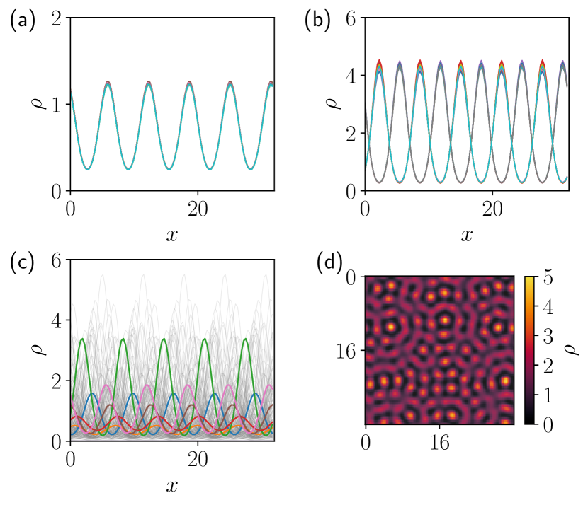
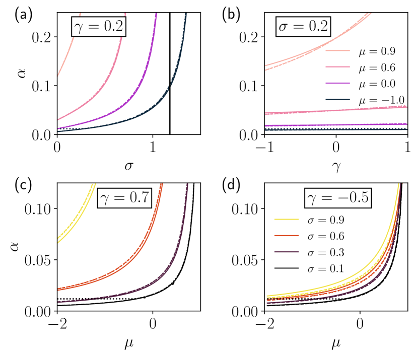
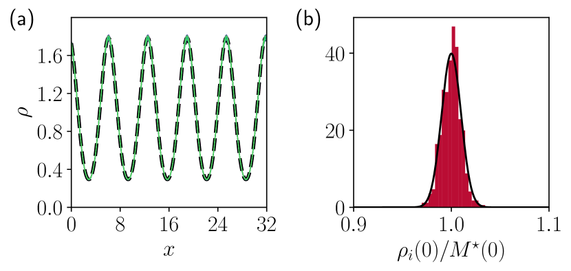
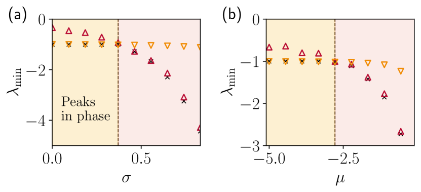
We then perform extensive numerical simulations to explore the phase diagram. In practice, and to keep a reasonable convergence time, we solve the dynamics via a semi-spectral scheme on a one-dimensional domain with periodic boundary conditions, for . We first confirm that for , the homogeneous state remains stable, see symbols Fig. 3(a) and (d). We then identify 3 regimes when the homogeneous state loses stability via , i.e. when . (i) For small values of the dispersion , the system can reach a stationary state where all the species densities display spatial modulation of wavelength , as displayed in Fig. 2(a) and (b). (ii) For larger values of and , the density profiles keep the patterned structure but are evolving with time. They typically oscillate, and the species propagate in the medium, without displaying mass explosion, see Fig. 2(c). (iii) For even larger values of , the instability at leads to exponential divergence of the pattern amplitudes and the abundances explode, see symbols () in Fig. 3(a) and (d).
Our numerical findings are consistent with our theory. They are also in agreement with the linking between scales observed numerically in [14], since our variable shows that the system will pattern when diffusion is small enough or when the range of interaction is large enough.
III.4 Surviving fraction and abundances
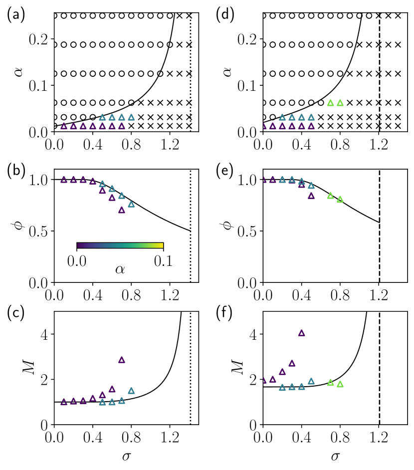
An important question that initially motivated this work is to know whether the additional spatial dimension may prevent species from becoming extinct. We hypothesized that moving in space could allow a species to escape a predator or to escape the competitive interactions on a given site. To measure the effect of space on the ecosystem, we rely on two observables, namely, the surviving fraction and the mean abundance . In the system, a species is considered surviving if its mean abundance over space denoted is larger to some threshold, typically . The surviving fraction is the ratio of the number of surviving species denoted and the total number of species .
Interestingly enough, we find that the surviving fraction when species can spread spatially is not higher than the surviving fraction of the zero-dimensional system, when species are forced to interact in the same point of space. This is shown in Fig. 3(b) and (c) where the results of the simulations closely follow the prediction of in a zero-dimensional system. Even in the case of cooperative interactions (), the surviving fraction is bounded by the 0d prediction. For very low the surviving fraction is even smaller than the 0d prediction. On the other hand, the mean abundance of the species across space, defined as is found to be significantly larger than the 0d prediction for small , see Fig. 3(c) and (f). As increases, the abundances eventually diverge while the density profiles keep their spatially-periodic structure. All in all, our results indicate that space allows for a diverging biomass for lower levels of heterogeneity in the interactions. This fact contrasts with those of [26, 27]. Even though survival fraction increases with diffusion (higher values of ), in our case average mass, , decreases for larger diffusion, as it can be seen in Fig. 3.
IV F-KPP equations and stable patterns
In the previous section, we have shown that the flat solution was destabilized for . However, a proof is missing confirming the convergence to some state, stationary or not, in which the species densities remain bounded. We address this question below.
IV.1 The limit case
Confirming the existence of a patterned solution to a partial differential equation can usually be done via the amplitude equation describing the evolution of the large wavelength modulations of the sinusoidal patterns emerging at the critical wavelength . For , the disorder on the interacting coefficients can lead to oscillations and non-stationary solutions, as shown by the PDE solutions. To get insights on the dynamics and to capture the transitions that we observe, we derive the DMFT equation describing the typical behavior of a random species in the ecosystem. This derivation is carried out in Appendix C. Finding a complete ansatz for the DMFT equation is usually out of reach in the general case. For however, the disorder only lies in the initial conditions, and the DMFT equation can be strongly simplified, as the self-consistent noise and the response term vanish. The dynamics of a typical species thus reads
| (16) | ||||
Since the noise has vanished, all species now follow the same evolution equation. If , species are not interacting with each other, and their final density profile will be identical, up to some phase shift that depends on the initial conditions. In particular, each species density satisfies a nonlocal Fisher-Kolmogorov-Petrovskii-Piskunov (F-KPP) equation [38, 39, 40], whose stationary fixed point is either homogeneous or patterned [41]. In , the stationary patterns span on the whole spatial domain and are pure sinusoids close to the onset, and in a species condenses in a triangular lattice. For , the different species do interact and we can assume that the initial conditions will not be relevant anymore to determine the density profile at long times. Numerically, we observe two distinct behaviors, depending on the sign of .
For (competitive interactions), the species end up all overlapping into a single stationary patterned state, similarly to what is shown in Fig. 2(a) in , or on the same triangular lattice in (not shown). In that case, the species profiles cannot be distinguished from the mean . If one assumes that, indeed, each profile can then be expanded as , one obtains to leading order the dynamics for the mean:
| (17) | ||||
and we recover a nonlocal F-KPP equation, now satisfied for the mean . A solution to this equation is a stationary patterned profile, that we will denote , for which densities remain bounded. In our case , close to the onset of patterning, the modes of interest are all around [41], where is defined by Eq. (8).
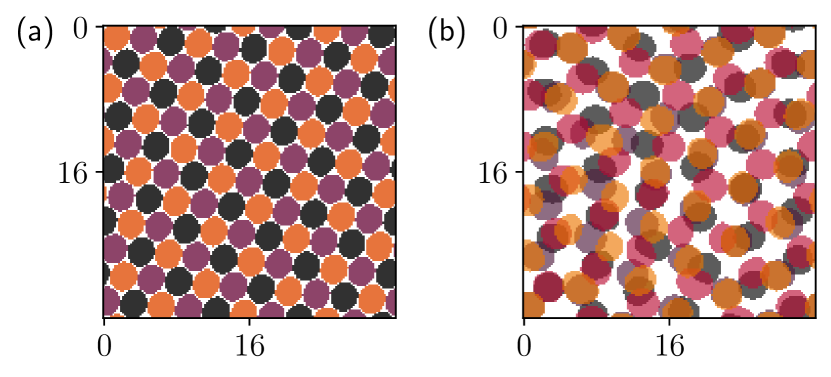
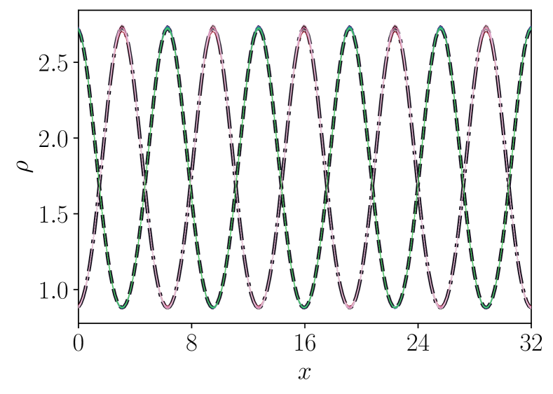
For (cooperative interactions), the species spread spatially and self-organize into two groups (in ) with identical static pattern profiles (one group density is shifted by half a period with respect to the other), similarly to what is shown in Fig. 2(b). In dimensions, group repulsion is also found but the species may end up in a frustrated state. Indeed, each species arranges in a triangular lattice but these lattices repel each other. For 3 species only, the lattices do not overlap because each species can occupy the nodes of a different triangular lattice, see Fig. 4(a). Once a fourth species is added, the new triangular lattice of this species is repelled by the 3 others. As the number of species increases, the frustration enhances the apparition of topological defects that suppress the long-range translational and rotational orders, see Fig. 4(b). In Fig. 2(d), we display the average density of species in this frustrated system.
The drastic change of behavior as changes sign is the signature of a phase transition. We relate the transition in the patterns to a transition in the spectrum of the matrix . We sketch the argument below. For , when the minimum eigenvalue of the matrix is and is of multiplicity , while for , and is of multiplicity , as detailed in Appendix D. The value corresponds to the outlier crossing the edge of the bulk of the spectrum (although degenerate for ), a second-order transition referred to as the Baik–Ben Arous-Péché (BBP) transition [42]. Focusing on the case , one can show that the eigenvector related to the outlier eigenvalue is . The function is then given by , the projection of the density vector on the only unstable direction that destabilizes all the species in the same direction. The species finally align and the only dynamically relevant equation is indeed the equation of the mean . For , there is no longer a unique unstable direction, and all the dynamically relevant directions (and equations) are to be considered, which translates in the PDE solution into several groups of interacting patterns.
It may appear paradoxical that the species split in several families when interactions are cooperative, while they overlap when they compete. We rationalize this behavior a posteriori when we compare the interaction radius of the kernel (here a step) to the period of the patterns . In particular, focusing in for simplicity, we have , which means that a species, labeled , that condenses at the maximum density of the patterns of a second one, labeled , will not interact with the other density peaks of the species , a favorable situations when species compete. Shifting the settlement of species by half of a period allows the species to interact with two density peaks of , beneficial for abundances when interactions are cooperative. The phenomenon described here is possible because the kernel somehow weights distant interactions as relevant as local ones, which is tightly related to the fact that its Fourier transform has negative values. And indeed, we have checked that this behavior is recovered with other kernels whose Fourier transforms display negative values. Finally, taking a nonzero such that an outlier eigenvalue can still exist in the spectrum should not change the global picture of the pattern transition. This is the subject of the next section.
IV.2 Expansion close to
IV.2.1 Case : instability from the outlier eigenvalue
What is the level of dispersion in the interactions for which the patterns are stable? We have shown in the previous paragraph that for , one can recover the nonlocal F-KPP equation satisfied by the mean . At the onset of patterning, we have shown that the solution is spatially oscillating with wavenumber , and that the patterns are static and stable. Our goal is now to expand for small but nonzero.
We start back from Eqs. (11) and (15), and we rescale , such that the quantity stays of order , and the critical line in parameter space is not collapsing on the axis in the limit . In that limit, the variance of the distribution of fixed points goes to zero, and the mean is . We are going to expand close to the solution. We have for some random species :
| (18) |
with a species dependent field. We use the fact that is solution of (17), and retaining leading order terms in the DMFT equation yields
| (19) | ||||
The DMFT noise , that satisfies , needs simply to be evaluated to leading order. The correlation now reads
| (20) | ||||
| (21) |
to leading order. The correlation is no longer a function of and , so it is constant in time. In space, the correlation is now factorized, which means that the covariance matrix is of rank 1. Hence, the noise , that is Gaussian, is now deterministic, once given. We drop the time dependence and we have
| (22) |
with a Gaussian random variable of mean 0 and variance 1. Injecting in Eq. (19), we have
| (23) | ||||
which accepts as a static solution. We are now able, using Eq. (18), to give an explicit formula for the density profiles close to :
| (24) |
We have thus explicitly shown that the patterns survive a small amount of disorder in the interaction. Moreover, the density fields of the different species are all proportional to the mean profile , and the dispersion around this profile is Gaussian with variance . Interestingly enough, this result holds even for , i.e. far from the onset of patterns, as shown in Fig. 5, where the amplitude of the patterns is of the same order as the mean density. Finally, although the system may display a time oscillating behavior and traveling waves, the prediction of such features is out of the scope of the present study, since they occur for larger and for which the noise can no longer be simplified as it has been here.
IV.2.2 Case : instability from the edge of the bulk
In that case, at , the system splits into two families (for ) of periodic fields and , of spatial periodicity , and that satisfy
| (25) | ||||
| (26) | ||||
with, in addition, . The density profile, that is a random variable, can be written
| (27) |
with , a random variable that satisfies exactly, according to the PDE solutions. The are thus correlated but the correlation vanishes in the limit.
We now look at a small expansion. The density is expanded as . The constraints on the noise correlation reads
| (28) | ||||
| (29) |
Since the noise is Gaussian, the covariance matrix of rank 2 fully determines the noise, which is then given by
| (30) |
with , independent Gaussian random variables of mean 0 and variance 1. One can show that the stationary solution for is not a simple linear combination of the two fields and , but rather involves nonlocal operators. As such, the stationary solution cannot be obtained explicitly. It has nonetheless the same flavor as the case, where each species follows one of the two master densities of , as displayed in Fig. 6. In particular, the variance of the Gaussian distribution of abundances around each of the master densities and is now space dependent.
IV.3 Larger values of
As the heterogeneity increases, mean cooperation or competition are lost in the noise of interactions with other species. As long as the instability at finite wavelength comes from the outlier eigenvalue of , species’ patterns are in phase close to the instability onset. Their amplitudes can be strongly spread however. When the outlier eigenvalue is absorbed by the bulk, patterns no longer share the same phase. The transition between the two regimes is given in Appendix D, and is summarized in Fig. 7 where the prediction of the outlier and the bulk minimum eigenvalue are compared.
V Conclusion
Let us summarize what we have achieved in this paper. Starting from a spatially-extended ecosystem of generalized Lotka-Volterra type where interactions between species are random but possibly correlated, we have computed the criterion for the loss of stability of the spatially homogeneous ecosystem. The instability at finite wavelength cannot develop if the Fourier transform of the interaction kernel is positive for all Fourier modes. The stability criterion depends on the most abundant species and can be captured by the ratio , that measures how far species diffuse in one generation with respect to the interspecies interaction range. If species move fast enough, the system remains homogeneous. As the homogeneous phase loses its stability, the stationary patterned profiles are solutions of a nonlocal F-KPP equation. In addition, we have identified a BBP transition at the linear stability level that translates in a transition in the stationary state, where nonlinear terms are relevant. Expanding in the heterogeneity level parameter close to the patterned state, we have shown that an explicit solution of the DMFT equation could still be obtained in the stationary regime.
From a theoretical point of view, our work suggests that combining approaches from active matter systems, theoretical ecology and disordered systems is a promising path to unveil salient features of the spatial organization of interacting species. In our work, we have mainly focused on the behavior at long times in a closed environment. The dynamics of spreading of the species in an unbounded domain remains to be explored. We have also discarded the noise coming from the spatial diffusion and the one coming from population dynamics, that should ultimately be considered to understand the invasion and the extinction of species. Experimentally, the dynamics of many interacting bacterial strains start to be scrutinized at the lab [43, 44, 45], and new experiments with genetically engineered strains, in the spirit of [46], offer a way to test the mechanism we have pinpointed that lead to pattern formation. In natural habitats, experiments are difficult to carry out, but data of quality are progressively obtained by means of environmental DNA [47, 48]. Accurate maps on the repartition of species offer a new way to test predictions based on the complex system approaches [49].
Acknowledgements.
We warmly thank A. Altieri, J.W. Baron, M. Benzaquen, J.-P. Bouchaud, and J. Garnier-Brun for interesting discussions and precious insights. R.Z. thanks T. Arnoulx de Pirey for illuminating discussions. This research was conducted within the Econophysics & Complex Systems Research Chair, under the aegis of the Fondation du Risque, the Fondation de l’École polytechnique, the École polytechnique and Capital Fund Management.Appendix A Generalization to non-feasible ecosystems
In general, given the interaction matrix , for large or for large , it is possible to show that species extinction necessary occurs [17]. The system is then said to be non-feasible. The results from the section III.2 might differ in this situation. We address this question below.
We consider a system that has undergone species extinction and we want to know if the final homogeneous state is stable with respect to spatial perturbation of the species abundances. The perturbation affects all the species, surviving ones as well as extinct ones (this can be justified if one allows species to migrate into the considered domain). For clarity, we reorder the species indices, such that, by denoting the number of surviving species, we have which refers to surviving species while will refer to extinct species. At the same time, we reorder the interaction matrix and we denote by the new interaction matrix that can be cast with 4 blocks:
| (31) |
with refers to the interactions of surviving species on other surviving species, the interactions of extinct species on extinct ones, and the interactions of surviving species on extinct ones. In particular, the blocks and are square matrices of size and , respectively. Considering a perturbation , the linearized dynamics of Eq. (1) reads
| (32) | ||||
where now one has to be careful of the fact that for , . In a compact form, one can write
| (33) |
with the matrix given by
| (34) |
and is the diagonal matrix of size with elements , the positive abundances of the surviving species. The stability is then determined by the spectrum of the operator . In particular, since is block upper triangular, its spectrum is the union of the spectrum of and the spectrum of . It turns out that the eigenvalues of are all necessarily negative since the extinct species have all died out dynamically in the homogeneous system by construction. The destabilization of the ecosystem can only come from the spectrum of . The work [22] has addressed the question of the boundaries of the spectrum of . Let us then discuss the stability depending on the sign of the kernel :
(i) If then . The matrix is referred to as the reduced Jacobian in Ref. [22]. It turns out that the leading eigenvalue (which is real) of the reduced Jacobian becomes positive exactly when the leading eigenvalue of the reduced interaction matrix becomes positive. However, as soon as the mode diverges. In other words, the reduced interaction matrix fully determines the stability in this case, and the spatially-extended system loses stability for the modes exactly when the zero-dimensional system loses stability. In this case we should not expect stable regular spatial heterogeneities.
(ii) If for some , one has , then . Using perturbation theory like in the feasible ecosystem case, we find that one has
| (35) |
Again, the stability is set by the most abundant species.
Appendix B Known results in the zero-dimensional case
We recall here the known results on the distribution of fixed points and the system stability when , as it can be found in [50, 51]. We consider a generalized Lotka-Volterra dynamics in zero dimension
| (36) |
where a perturbation field has been introduced for convenience to compute the response to a perturbation on the dynamics. Via the cavity method (sketched in the next section) or via the generating functional analysis, one obtains the DMFT equation. This equation pinpoints the role of 3 observables that self-consistently determine the dynamics. We define the mean abundance of the species
| (37) |
the correlation of the species abundance,
| (38) |
and the response function
| (39) |
Assuming that we lie in the region of parameters where the system has converged to a stationary state, the final abundance of a species is a random variable that we denote . The first and the second moment of the distribution are then denoted , , and the static response function is denoted . Defining , one obtains , and as the solution of the self-consistent equations:
| (40) | ||||
| (41) | ||||
| (42) |
and . In Ref. [17], the distribution of fixed points is computed and reads
| (43) |
with the Heaviside function and a Gaussian random variable of mean and variance . The complete distribution of thus splits between the surviving species (of fraction ) with distribution , and the extinct species of fraction .
Appendix C Dynamical-mean-field theory equations
In the main text, the phase diagram has been obtained using perturbation analysis, valid only at order 1 in . We have also used results from dynamical-mean field theory obtained in zero dimension [17]. In what follows we will generalize the DMFT equation in dimension and see what one can deduce from this set of self-consistent equations.
C.1 Sketch of the derivation for the DMFT equations
We derive the DMFT equations via the cavity method [52]. A new species in the system is considered as a perturbation of existing dynamics. Interactions between species are then interpreted as coming from a fluctuating bath. A set of an infinite number of deterministic equations simplifies into a single stochastic equation describing the density of a typical representative species in our system. We refer the reader to [53] where similar derivations are carried out in a pedestrian way. Starting from our set of equations describing the evolution of species,
| (44) | ||||
and we introduced an auxiliary field , later set to zero, that provides the response and correlation functions necessary to close the dynamics.
We now follow the common steps of the DMFT to obtain the self-consistent equation:
1. Let the be solutions of the system (44).
2. Add a new species, labeled with index , which follows a similar dynamics:
| (45) | ||||
where the are the solutions of the dynamics that includes interactions with species .
3. For large enough, the effect of a new species on the dynamics is small and can thus be treated via linear perturbation theory. The perturbed trajectories are thus given by
| (46) |
where denotes the response function.
4. We can insert Eq. (46) into Eq. (45) to obtain
| (47) | ||||
with
| (48) | ||||
| (49) |
5. This latter equation can simplify when using the correlations between the matrix coefficients of , invoking the central limit theorem and neglecting terms scaling in , see [51].
6. We finally obtain the evolution equation of the density , but since all species play a similar role, encodes in fact the “typical” behavior any species in the system. We thus drop the index and the evolution equation reads
| (50) |
where , is a Gaussian noise with space and time correlation
| (51) |
and the response function
| (52) |
The average is taken over several realizations of the complete dynamics (1).
C.2 Fixed points and stability analysis
There are a priori two kinds of fixed points in the DMFT: homogeneous fixed points, denoted and non-homogeneous ones, . Looking for homogeneous fixed points is equivalent to finding the ones from the zero-dimensional model, already presented in Appendix B.
On the other hand, we can find necessary conditions to the existence of a spatially dependent stationary state . Such a state would indeed solve the time-independent version of Eq. (50), and one solution has been obtained for small and . Determining the stability of such solutions via a DMFT linear stability analysis cannot be performed easily because of products of space-dependent fields that hinder modes diagonalization via Fourier transforms. Nonetheless, we suggest to follow a general path to assess state stability and will refine hypotheses later.
A natural procedure to assess the stability is to perturb the system with a multiplicative Gaussian white noise (with ) such that the perturbed dynamics still satisfies . One then computes the power spectrum of the field that is continuously kicked away from the fixed points by the excitations. As we expect to stay close to the fixed point solution, we write and as
| (53) | ||||
| (54) |
with , , , , and the self-consistent correlation relations
| (55) | ||||
| (56) |
where averaging over the white noise , the DMFT noise and the distribution of fixed points is indicated by the indices of the brackets. A step-by-step treatment of the different terms can be found in the lecture notes of Galla, see [51]. Retaining leading order terms in Eq. (50) leads to linear equations for . In particular, close to the identically zero fixed points , one obtains
| (57) |
We note first that the perturbations around the identically (flat) zero fixed point vanish. Indeed in Fourier space the relaxation rate of a Fourier mode reads , with since from the truncated Gaussian distribution in (43). On the other hand, the fluctuations around a non-zero fixed point satisfy
| (58) | ||||
A comprehensive study of this equation with a space dependent fixed point would be out of the scope of the present work. In the following we will focus on the perturbations around homogeneous nonzero fixed points. Close to a homogeneous state of density , the dynamics (58) in Fourier space reads
| (59) | ||||
which, after factorizing, yields
| (60) | ||||
The power spectrum is obtained by taking the modulus squared and the average over the independent noises , DMFT noise , and realizations of fixed point . In particular, the contributions to the spectrum from the vanishes, which explicitly writes
| (61) | ||||
| (62) | ||||
| (63) | ||||
Using now the independence of , and , and using Eq. (56), one obtains
| (64) |
with
| (65) |
and we check that for , the power spectrum remains finite. The solution to reads
| (66) |
We now take the limit to probe the behavior of the spectrum at long times, and we will denote , and , which is real. We check that taking the limit yields back the power spectrum of the zero-dimensional case investigated in [50, 16, 17], that reads
| (67) |
and which diverges when one has , with . Keeping the mode dependence, the onset of instability of the system is the manifold on which the power spectrum starts diverging. The condition yields the fastest growing mode and reads
| (68) |
with
| (69) | ||||
and where we defined
| (70) |
Equation (69) can be further simplified. Indeed, through Eq. (60), we have, by definition of the response function,
| (71) | ||||
| (72) |
By taking the derivative with respect to in Eq. (72) (and taking ), one obtains
| (73) | ||||
Injecting this expression in Eq. (69), we find that only if solves . We thus recover here the condition of Eq. (8) on the critical mode that we obtained from the linear stability analysis conducted in Section III.2. Finally using a mean-field approximation in Eq. (72), we find that is a root of a second-degree polynomial, which leads to
| (74) |
This expression can then be injected into in order to solve the instability criterion .
We now examine the case where can be negative and we focus on the fastest growing mode , for which necessarily. One would like to assess the expectation , but one notices that there is a pole in the integrand of that leads to divergence of as soon as the support of the distribution of intercepts it. In addition, since for modes that satisfy , the function is surjective on , hence there exists a mode such that Eq. (66) is satisfied, yielding the divergence of the power spectrum for that mode. In other words, the system is always unstable when the number of species goes to infinity, in line with our findings of Section III.3.
To avoid the trivial divergence of the dynamics, we finally consider a large but finite system , and it is interesting to restrict the integration bound on to the highest abundance that can be obtained from draws on the fixed point distribution. Denoting by , we define
| (75) |
If , then remains finite and is maximal for , see Eq. (68). Hence we have
| (76) |
and the power spectrum diverges as soon as
| (77) |
This equation can be solved numerically to recover the transition line in parameter space , see Fig. 1. The agreement between the DMFT and the perturbation theory is remarkable.
Appendix D Exact results from random matrix theory
In the presence of the interaction kernel , we have seen that the stability of the ecosystem is determined by the minimal eigenvalue of the matrix . We are computing this minimal eigenvalue in what follows.
We first write the matrix in the following way,
| (78) |
with and the matrix filled of , and such that it is clear that the effect of is that of a rank one perturbation in the limit.
Consider first the case . The species are all equivalent, and , with . The spectrum can be computed analytically, and the eigenvalues are simply
| (79) |
This means that asymptotically we have eigenvalues equal to and one eigenvalue equal to . Therefore, the minimum depends on the sign of ,
| (80) |
The general case will behave in a similar way. It is useful to first consider the case , and . We will generalize to the case later.
We introduce the resolvent for the matrix ,
| (81) |
and its trace,
| (82) |
The function encodes the information about the eigenvalues of in its poles. We will approximate it by means of the cavity method. Using the Schur complement formula, we have
| (83) |
where is the resolvent for the matrix with row and column removed. Using the Schur complement a second time we can write an equations for it as well,
| (84) |
In the large limit we can use the statistical properties of the variables and assume statistical properties of will be independent of the removed site, , giving
| (85) |
where
| (86) |
Plugging this back in (83), we get
| (87) |
In order to write a self-consistent equation for we assume statistical equivalence between and , which should hold in the large limit, combining this with (84) and (86) we write down the following equation,
| (88) |
We can immediately see that for , can be approximated with
| (89) |
and the poles are all simply located at the values . Since we are interested in the minimum eigenvalue of , we can see it has to be associated with , giving .
Now assume that for moderate , the minimum eigenvalue is real and just slightly perturbed, , we can write down the equation for assuming it is associated with a new pole, ,
| (90) |
While (88) and (90) constitute a well-defined system of equations for and , we can proceed further analytically if we perform a mean-field approximation for ,
| (91) |
where . This function has a simple analytical form,
| (92) |
Note that we have precisely recovered the response function obtained in Eq. (74), if one sets . Using (92) with (90) we can derive
| (93) |
where we have used the fact for large by definition of . All in all, the minimal eigenvalue reads
| (94) |
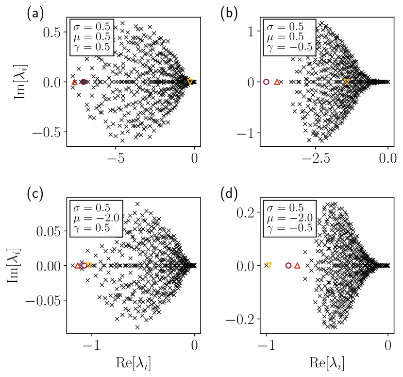
Comparison with the order 0 perturbation theory is displayed in Fig. 8 where the full spectrum of the matrix is computed for various , and . There, the matrix is obtained from running the 0-dimensional Lotka-Volterra dynamics given by . Hence, the matrices and are not independent, but assuming they are is indeed a very good approximation.
For the outlier we can follow similar steps as in [54]. The outlier eigenvalue should satisfy by definition , which here writes
| (95) |
If is outside of the bulk then we should have invertible, giving
| (96) |
using Sylvester’s determinant theorem
| (97) |
where by definition we have
| (98) |
If we approximate by keeping only the diagonal terms when is small and use definition (86), we find the following equation for the outlier eigenvalue,
| (99) |
Using the mean-field approximation, (92), we find
| (100) |
Note that this formula uses both a mean-field and a diagonal approximation, but the outlier is properly predicted for large values of and , as shown in Fig. 7. Also, the formula is no longer valid if . Finally equating the outlier eigenvalue and the minimum eigenvalue of the bulk obtained in Eq. (94) yields the approximated frontier of the BBP transition.
References
- Lotka [1920] A. J. Lotka, Undamped oscillations derived from the law of mass action., Journal of the american chemical society 42, 1595 (1920).
- Volterra [1926] V. Volterra, Fluctuations in the abundance of a species considered mathematically, Nature 118, 558 (1926).
- Maslov and Sneppen [2017] S. Maslov and K. Sneppen, Population cycles and species diversity in dynamic kill-the-winner model of microbial ecosystems, Scientific reports 7, 1 (2017).
- Joseph et al. [2020] T. A. Joseph, L. Shenhav, J. B. Xavier, E. Halperin, and I. Pe’er, Compositional lotka-volterra describes microbial dynamics in the simplex, PLoS computational biology 16, e1007917 (2020).
- Dedrick et al. [2023] S. Dedrick, V. Warrier, K. P. Lemon, and B. Momeni, When does a Lotka-Volterra model represent microbial interactions? Insights from in vitro nasal bacterial communities, mSystems 8, e0075722 (2023).
- Fisher [1937] R. A. Fisher, The Wave of Advance of Advantageous Genes, Annals of Eugenics 7, 355 (1937).
- Kolmogorov et al. [1937] A. Kolmogorov, I. Petrovsky, and N. Piskunov, Investigation of a diffusion equation connected to the growth of materials, and application to a problem in biology, Bull. Univ. Moscow, Ser. Int. Sec. A 1 (1937).
- Reichenbach et al. [2008] T. Reichenbach, M. Mobilia, and E. Frey, Self-organization of mobile populations in cyclic competition, Journal of Theoretical Biology 254, 368 (2008).
- Täuber [2024] U. C. Täuber, Stochastic spatial lotka-volterra predator-prey models (2024), arXiv:2405.05006 [cond-mat.stat-mech] .
- Deforet et al. [2019] M. Deforet, C. Carmona-Fontaine, K. S. Korolev, and J. B. Xavier, Evolution at the edge of expanding populations, The American Naturalist 194, 291 (2019), pMID: 31553215.
- Lee et al. [2022] H. Lee, J. Gore, and K. S. Korolev, Slow expanders invade by forming dented fronts in microbial colonies, Proceedings of the National Academy of Sciences 119, e2108653119 (2022).
- Pigolotti et al. [2007] S. Pigolotti, C. López, and E. Hernández-García, Species Clustering in Competitive Lotka-Volterra Models, Physical Review Letters 98, 258101 (2007).
- Andreguetto Maciel and Martinez-Garcia [2021] G. Andreguetto Maciel and R. Martinez-Garcia, Enhanced species coexistence in Lotka-Volterra competition models due to nonlocal interactions, Journal of Theoretical Biology 530, 110872 (2021).
- Zelnik et al. [2024a] Y. R. Zelnik, M. Barbier, D. W. Shanafelt, M. Loreau, and R. M. Germain, Linking intrinsic scales of ecological processes to characteristic scales of biodiversity and functioning patterns, Oikos 2024, e10514 (2024a).
- May [1972] R. M. May, Will a Large Complex System be Stable?, Nature 238, 413 (1972).
- Bunin [2017] G. Bunin, Ecological communities with Lotka-Volterra dynamics, Physical Review E 95, 042414 (2017).
- Galla [2018] T. Galla, Dynamically evolved community size and stability of random Lotka-Volterra ecosystems, Europhysics Letters 123, 48004 (2018).
- Altieri et al. [2021a] A. Altieri, F. Roy, C. Cammarota, and G. Biroli, Properties of equilibria and glassy phases of the random lotka-volterra model with demographic noise, Phys. Rev. Lett. 126, 258301 (2021a).
- Aguirre-López [2024] F. Aguirre-López, Heterogeneous mean-field analysis of the generalized lotka-volterra model on a network, arXiv preprint arXiv:2404.11164 (2024).
- Poley et al. [2024] L. Poley, T. Galla, and J. W. Baron, Interaction networks in persistent lotka-volterra communities, arXiv preprint arXiv:2404.08600 (2024).
- Park et al. [2024] J. I. Park, D.-S. Lee, S. H. Lee, and H. J. Park, Incorporating heterogeneous interactions for ecological biodiversity, Physical Review Letters 133, 198402 (2024).
- Baron et al. [2023] J. W. Baron, T. J. Jewell, C. Ryder, and T. Galla, Breakdown of Random-Matrix Universality in Persistent Lotka-Volterra Communities, Physical Review Letters 130, 137401 (2023).
- Arnoulx de Pirey and Bunin [2023] T. Arnoulx de Pirey and G. Bunin, Aging by Near-Extinctions in Many-Variable Interacting Populations, Physical Review Letters 130, 098401 (2023).
- Suweis et al. [2024] S. Suweis, F. Ferraro, C. Grilletta, S. Azaele, and A. Maritan, Generalized lotka-volterra systems with time correlated stochastic interactions, Physical Review Letters 133, 167101 (2024).
- Arnoulx de Pirey and Bunin [2024] T. Arnoulx de Pirey and G. Bunin, Many-Species Ecological Fluctuations as a Jump Process from the Brink of Extinction, Physical Review X 14, 011037 (2024).
- Garcia Lorenzana et al. [2024] G. Garcia Lorenzana, A. Altieri, and G. Biroli, Interactions and migration rescuing ecological diversity, PRX Life 2, 013014 (2024).
- Denk and Hallatschek [2024] J. Denk and O. Hallatschek, Tipping points emerge from weak mutualism in metacommunities, PLOS Computational Biology 20, 1 (2024), publisher: Public Library of Science.
- Olmeda and Rulands [2023] F. Olmeda and S. Rulands, Long-range interactions and disorder facilitate pattern formation in spatial complex systems, arXiv preprint arXiv:2303.12611 (2023).
- Padmanabha et al. [2024] P. Padmanabha, G. Nicoletti, D. Bernardi, S. Suweis, S. Azaele, A. Rinaldo, and A. Maritan, Landscape and environmental heterogeneity support coexistence in competitive metacommunities, Proceedings of the National Academy of Sciences 121, e2410932121 (2024).
- Galla [2006] T. Galla, Random replicators with asymmetric couplings, Journal of Physics A: Mathematical and General 39, 3853 (2006).
- Altieri et al. [2021b] A. Altieri, F. Roy, C. Cammarota, and G. Biroli, Properties of Equilibria and Glassy Phases of the Random Lotka-Volterra Model with Demographic Noise, Physical Review Letters 126, 258301 (2021b).
- Garnier-Brun et al. [2021] J. Garnier-Brun, M. Benzaquen, S. Ciliberti, and J.-P. Bouchaud, A new spin on optimal portfolios and ecological equilibria, Journal of Statistical Mechanics: Theory and Experiment 2021, 093408 (2021).
- Ahmadian et al. [2015] Y. Ahmadian, F. Fumarola, and K. D. Miller, Properties of networks with partially structured and partially random connectivity, Phys. Rev. E 91, 012820 (2015).
- Stone [2018] L. Stone, The feasibility and stability of large complex biological networks: a random matrix approach, Scientific Reports 8, 8246 (2018).
- Tuck [2006] E. Tuck, On Positivity of Fourier Transforms, Bulletin of the Australian Mathematical Society 74, 133 (2006).
- Giraud and Peschanski [2014] B. G. Giraud and R. Peschanski, On the positivity of Fourier transforms, Tech. Rep. arXiv:1405.3155 (arXiv, 2014) arXiv:1405.3155 [hep-ph, physics:hep-th, physics:math-ph, physics:nucl-th] type: article.
- Turing [1990] A. M. Turing, The chemical basis of morphogenesis, Bulletin of mathematical biology 52, 153 (1990).
- Berestycki et al. [2009] H. Berestycki, G. Nadin, B. Perthame, and L. Ryzhik, The non-local Fisher–KPP equation: travelling waves and steady states, Nonlinearity 22, 2813 (2009).
- Achleitner and Kuehn [2015] F. Achleitner and C. Kuehn, On bounded positive stationary solutions for a nonlocal Fisher–KPP equation, Nonlinear Analysis: Theory, Methods & Applications 112, 15 (2015).
- Kuehn and Throm [2018] C. Kuehn and S. Throm, Validity of amplitude equations for nonlocal nonlinearities, Journal of Mathematical Physics 59, 071510 (2018).
- Faye and Holzer [2015] G. Faye and M. Holzer, Modulated traveling fronts for a nonlocal Fisher-KPP equation: A dynamical systems approach, Journal of Differential Equations 258, 2257 (2015).
- Baik et al. [2005] J. Baik, G. B. Arous, and S. Péché, Phase transition of the largest eigenvalue for nonnull complex sample covariance matrices, The Annals of Probability 33, 1643 (2005).
- Monmeyran et al. [2021] A. Monmeyran, W. Benyoussef, P. Thomen, N. Dahmane, A. Baliarda, M. Jules, S. Aymerich, and N. Henry, Four species of bacteria deterministically assemble to form a stable biofilm in a millifluidic channel, npj Biofilms and Microbiomes 7, 64 (2021).
- Hu et al. [2022] J. Hu, D. R. Amor, M. Barbier, G. Bunin, and J. Gore, Emergent phases of ecological diversity and dynamics mapped in microcosms, Science 378, 85 (2022).
- Alejandro Martínez-Calvo et al. [2023] Alejandro Martínez-Calvo, Carolina Trenado-Yuste, Hyunseok Lee, Jeff Gore, Ned S. Wingreen, and Sujit S. Datta, Interfacial morphodynamics of proliferating microbial communities, bioRxiv , 2023.10.23.563665 (2023).
- Curatolo et al. [2020] A. Curatolo, N. Zhou, Y. Zhao, C. Liu, A. Daerr, J. Tailleur, and J. Huang, Cooperative pattern formation in multi-component bacterial systems through reciprocal motility regulation, Nature Physics 16, 1152 (2020).
- Bohmann et al. [2014] K. Bohmann, A. Evans, M. T. P. Gilbert, G. R. Carvalho, S. Creer, M. Knapp, W. Y. Douglas, and M. De Bruyn, Environmental dna for wildlife biology and biodiversity monitoring, Trends in ecology & evolution 29, 358 (2014).
- Aglieri et al. [2021] G. Aglieri, C. Baillie, S. Mariani, C. Cattano, A. Calò, G. Turco, D. Spatafora, A. Di Franco, M. Di Lorenzo, P. Guidetti, et al., Environmental dna effectively captures functional diversity of coastal fish communities, Molecular Ecology 30, 3127 (2021).
- Zelnik et al. [2024b] Y. R. Zelnik, N. Galiana, M. Barbier, M. Loreau, E. Galbraith, and J.-F. Arnoldi, How collectively integrated are ecological communities?, Ecology Letters 27, e14358 (2024b).
- Opper and Diederich [1992] M. Opper and S. Diederich, Phase transition and 1/ f noise in a game dynamical model, Physical Review Letters 69, 1616 (1992).
- Galla [2024] T. Galla, Generating-functional analysis of random lotka-volterra systems: A step-by-step guide (2024), arXiv:2405.14289 [cond-mat.dis-nn] .
- Mézard et al. [1987] M. Mézard, G. Parisi, and M. A. Virasoro, Spin glass theory and beyond: An Introduction to the Replica Method and Its Applications, Vol. 9 (World Scientific Publishing Company, 1987).
- Roy et al. [2019] F. Roy, G. Biroli, G. Bunin, and C. Cammarota, Numerical implementation of dynamical mean field theory for disordered systems: application to the lotka–volterra model of ecosystems, Journal of Physics A: Mathematical and Theoretical 52, 484001 (2019).
- Baron [2022] J. W. Baron, Eigenvalue spectra and stability of directed complex networks, Physical Review E 106, 064302 (2022).