Concentration of Empirical First-Passage Times

Abstract

First-passage properties are central to the kinetics of target-search processes. Theoretical approaches so far primarily focused on predicting first-passage statistics for a given process or model. In practice, however, one faces the reverse problem of inferring first-passage statistics from, typically sub-sampled, experimental or simulation data. Obtaining trustworthy estimates from under-sampled data and unknown underlying dynamics remains a daunting task, and the assessment of the uncertainty is imperative. In this chapter, we highlight recent progress in understanding and controlling finite-sample effects in empirical first-passage times of reversible Markov processes. Precisely, we present concentration inequalities bounding from above the deviations of the sample mean for any sample size from the true mean first-passage time and construct non-asymptotic confidence intervals. Moreover, we present two-sided bounds on the range of fluctuations, i.e, deviations of the expected maximum and minimum from the mean in any given sample, which control uncertainty even in situations where the mean is a priori not a sufficient statistic.

1 Introduction

In the past decades, there has been a surge of interest in target-search problems, typically devoted to determining the time it takes a random searcher to find a target. This stochastic time, canonically referred to as first-passage or first-hitting time, has proven to be invaluable in understanding kinetic properties of various physical, chemical, and biological processes redner2001guide ; metzler2014first ; lindenberg2019 ; iyer2016first ; Zhang2016 .

As a pioneering example consider diffusive barrier crossing, when a thermally driven searcher (e.g., a reactant molecule) must overcome an energy barrier in order to “collide” with its reaction or binding partner. This situation arises naturally in the classical picture of Kramers’ reaction-rate theory Kramers ; Haenggi , according to which kinetic rates of chemical reactions can be understood in terms of inverse mean first-crossing times. Building on the success of these ideas, first-passage theory remained an effective paradigm for investigating (bio-) chemical kinetics ever since Szabo ; Redner ; Grebenkov_2018 ; Grebenkov_2018_2 ; Grebenkov_PRL1 ; Bressloff ; Roldn2016 ; Ghusinga2017 ; Rijal2022 ; Parmar2015 ; Charlebois2011 ; Frey2019 ; Lloyd2001 ; Hufnagel2004 ; Olivier_RMP ; Boccardo2022 ; Erdmann2004_2 ; Thirumalai ; Blom2021 ; Goychuk2002 .

In a similar vein, numerous events in biological settings are initiated when a diffusing searcher, for example, a messenger ligand, first binds to its target, its receptor. Evidently, this prompts the application of first-passage ideas to study the kinetics of molecular and cellular processes such as cell signaling and gene regulation Berg ; Andy ; Holcman ; Olivier_Chromatin ; Marklund ; Bauer ; Olivier_NC ; Bnichou2014 ; Godec_PRX ; Newby_PRL , intracellular transport Bressloff , RNA biosynthesis Roldn2016 , stochastic protein accumulation Ghusinga2017 ; Rijal2022 , DNA-binding Parmar2015 , virus uptake Frey2019 , cell adhesion Erdmann2004_2 ; Thirumalai ; Blom2021 , kinetochore capture Nayak2020 , or gating of ion channels Goychuk2002 . Notably, going beyond the molecular and cellular scope, first-passage principles have also found biological relevance in exploring the emergence of drug resistance Charlebois2011 , spreading dynamics of diseases Lloyd2001 ; Hufnagel2004 , and foraging behavior of bacteria and animals Olivier_RMP .

It should thus come to no surprise that addressing target-search questions through the lens of first-passage properties led to an immense body of literature with successful applications spanning virtually all scientific domains, including mathematics, physics, chemistry, biology, geology, economics, and finance, among others (see e.g. redner2001guide ; metzler2014first ; lindenberg2019 ; schuss2009theory ; bouchaud2003theory ; Paul2013 ; Gardiner and references therein).

First-passage concepts have further been applied in more abstract settings to characterize persistence properties Dougherty2002 ; Constantin2003 ; Merikoski2003 ; Constantin2004 ; Dougherty2005 ; Godrche2009 ; Bray_2013 , as well as diffusion through interfaces Kay2022 and across phase boundaries Bo2021 . Recently, first-passage problems arose in the field of stochastic thermodynamics Seifert2012 where they give insight into the statistics of stochastic currents currents ; Singh2019 , thermodynamic entropy production decision ; stopping ; Falasco2020 ; Neri2022 , and dynamical activity Garrahan2017 ; Hiura2021 in systems driven far from equilibrium. Lastly, we remark that first-passage phenomena are intimately tied to the statistics of extremes Kac ; Schehr ; Satya_records ; Hartich_JPA , and their mathematical description has been extended to capture quantum systems Eli_QM1 ; Eli_QM , additive functionals of stochastic paths Kearney2005 ; Kearney2007 ; Kearney2014 ; Kearney2021 ; Majumdar2021 ; Singh2022 , intermittent targets MercadoVsquez2019 ; Kumar2021 ; Spouge1996 ; Scher2021 ; Kumar2023 , active particles Woillez2019 ; Mori2020 ; DiTrapani2023 , non-Markovian dynamics Hnggi1983 ; Hanggi1985 ; Gurin2016 , and resetting processes Evans2011 ; Kusmierz2014 ; Reuveni2016 ; Pal2017 ; Pal2019 ; Evans2020 ; Besga2020 ; TalFriedman2020 ; DeBruyne2020 ; DeBruyne2022 ; Stojkoski2022 , including soft resets Deng2022 .

Unfortunately, the exact first-passage time density and thus the full statistics are typically known only for rather elementary examples and simple geometries (e.g., see Ref. redner2001guide ), and therefore remains a grand theoretical challenge on its own. The long-time behavior of the first-passage time density is generally somewhat better accessible but still requires substantial efforts Hartich_JPA ; Hartich_2018 ; Hartich_2019 . A more accessible, albeit still demanding, statistic is the mean first-passage time. Remarkably, this simplest statistic is often a highly non-trivial quantity, especially in cases where the dynamics span a broad range of timescales. Here, some trajectories almost directly reach the target and contribute to the short-time behavior, whereas others survive much longer and feed into the long-time behavior Godec_PRX . This makes an estimation of the mean first-passage time or its inverse (i.e., the kinetic rate constant) from experimental or simulation data a complex problem. The central theme of this chapter is thus how to efficiently control the uncertainty of such empirically derived estimates of the mean first-passage time, especially in the context of small sample-sizes.

We will focus on the first-passage properties of general target searches described by reversible Markovian dynamics in discrete or continuous state-spaces (see Fig. 1). In particular, we will discuss Markov jump processes with arbitrary transition-rate matrices and effectively one-dimensional diffusion processes in arbitrary confining potentials $U(x)$ that also include radial representations of hyper-spherically symmetric diffusion processes in $d$ dimensions where the spurious drift in radial direction allows the mapping to a one-dimensional geometric free energy of purely entropic origin (e.g., see Godec_PRX ).

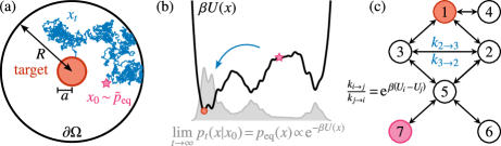
Figure 1: Schematic of target search processes for ergodic reversible Markov dynamics. Diffusive dynamics in (a) $d$ dimensional spherical domains (here $d=2$) with reflecting boundary $\partial\Omega$ and (b) arbitrary one-dimensional confining potential landscapes $U(x)$. (c) Markov jump dynamics on a discrete network state-space with transition rates that obey detailed balance. Search processes are initialized from $x_{t=0}$ (magenta), which is drawn from the stationary density $\tilde{p}_{\rm eq}(x)$ and we consider the first-passage time $\tau$ to reach the target (red).

The chapter is structured as follows. We begin in Sec. 2.1 with an overview of general first-passage concepts. In Sec. 2.2 we outline the basics of spectral theory of first-passage processes. Two illustrative examples are worked out in Secs. 2.3 and 2.4. Section 3 introduces the challenges associated with estimating mean first-passage times from observations, and Sec. 3.1 explores concentration inequalities for bounding deviations of inferred estimates from the true mean first-passage time, applicable for all sample sizes. Building on these results, Section 3.2 demonstrates how they can be applied to construct performance guarantees that do not hinge on asymptotic assumptions. In Section 4 we move beyond mean first-passage times and showcase results that bound deviations of minimum and maximum first-passage times in samples of arbitrary sizes. These findings are relevant in situations when the mean is a priori an insufficient statistic and problems involving multiple searchers. The chapter concludes in Sec. 5 with a discussion and an outlook.

2 First-passage fundamentals: a spectral-theoretic perspective

In this section we present some background, by introducing elementary concepts of first-passage theory of target search. Of particular importance is hereby the mathematical structure encoded in a spectral decomposition of first-passage time densities, which will be the essential building block of derivations throughout the chapter.

2.1 Generic concepts in first-passage theory

Let $x_{t}$ denote the abstract trajectory of a “searcher” in a state space $\Omega$; for instance, it may correspond to the position coordinate of a diffusive particle confined within a spherical domain (see Fig. 1a), a particle exploring an arbitrary confining potential landscape $U(x)$ (see Fig. 1b), or a network-based representation of protein configurations in the search of the native conformational state during folding (see Fig. 1c). We suppose that $x_{t}$ follows a reversible Markovian equation of motion. A more precise formulation of reversible dynamics will be given at the end of this section. The description will be kept “light” and informal.

The time required for the searcher to make its first encounter with some predefined target $a\in\Omega$ starting from an initial condition distributed according to the density $p_{0}$ then corresponds to the first-passage time $\tau$, formally defined as,

$$\tau=\inf_{t}\left[t|x_{t}=a,p_{0}(x_{0})\right].$$ (1)

The stochastic nature of the underlying dynamics inherently renders the first-passage time a random variable that not only depends on the location of the target $a$ but also the initial position $x_{t=0}$ (drawn from $p_{0}(x)$). The complete statistics of $\tau$ is encoded in the so-called survival probability

$$S_{a}(t|x_{0})\equiv\mathbb{P}(\tau\geq t),$$ (2)

the probability that the searcher has not found the target by time $t$, i.e., the first-passage event has not yet occurred by $t$. The normalized probability flux into the target $a$ corresponds to the first-passage time density $\wp_{a}(t|x_{0})=\langle\delta(t-\tau[\{x_{t^{\prime}}\}]\rangle$, where $\langle\cdot\rangle$ represents the average over all first-passage paths $\{x_{t^{\prime}}\}_{0\leq t^{\prime}\leq\tau}$, i.e., paths that hit $a$ only once. By the fundamental theorem of calculus, the survival probability $S_{a}(t|x_{0})$ in Eq. (2) and the first-passage time density $\wp_{a}(t|x_{0})$ are related via

$$\wp_{a}(t|x_{0})=-\frac{\partial}{\partial t}S_{a}(t|x_{0}).$$ (3)

Assumptions about the dynamics We assume $x_{t}$ to be a strongly ergodic time-homogeneous Markov process on a continuous or discrete state space $\Omega$ with invariant (equilibrium) density $p_{\rm eq}(x)$. The transition probability density $p_{t}(x|x_{0})$ to find $x_{t}$ at $x$ at time $t$, given that it started from $x_{0}$, is given by $p_{t}(x|x_{0})={\rm e}^{\hat{L}t}\delta_{x_{0}}(x)$ where $\delta_{x_{0}}(x)$ denotes either the Dirac or Kronecker delta, depending on the specific state-space being considered, and the generator $\hat{L}$ is a linear reversible (dissipative) operator that is essentially self-adjoint (i.e., it is self-adjoint in some basis; e.g., the operator $\sqrt{p_{\rm eq}(x)}^{-1}\hat{L}\sqrt{p_{\rm eq}(x)}$ is self-adjoint).

In our context, $\hat{L}$ can take the form of a Markov-rate matrix or, equivalently, an effectively one-dimensional Fokker-Planck operator with discrete spectrum and real non-positive eigenvalues; obeying detailed balance in both cases. The effectively one-dimensional character of the process is crucial, as the theory in Sec. 2.2 builds on the renewal theorem Siegert1951 ; Hartich_2018 ; Hartich_2019 . For the latter to hold, a process starting from some $x_{0}$ must, before reaching the final state $x$, pass through the point-like target set $a$ that, however, has zero measure in $d\geq 2$. If we consider absorbing sets with positive measure, the renewal structure breaks down unless the symmetry allows a reduction to an effectively one-dimensional Markov dynamics. The results may even hold without this requirement, but are not covered by our proof. As we assume $x_{t}$ to be ergodic, $p_{t}$ reaches Boltzmann-Gibbs equilibrium for long times $\lim_{t\to\infty}p_{t}(x|x_{0})=p_{\rm eq}\propto\exp(-\beta U)$ with thermal energy $\beta^{-1}=k_{\rm B}T$. Lastly, a discrete and real spectrum of eigenvalue is ensured by assuming that $\hat{L}$ is (i) either bounded (Fig. 1c) (ii) $\Omega$ is finite with reflecting boundary $\partial\Omega$ (Fig. 1a) or (iii) that $\beta U(x)$ is sufficiently confining (Fig. 1b).

The processes discussed above are relaxation processes that conserve probability. In the first-passage setting one has to additionally introduce the absorbing target $x=a$, which formally modifies the generator $\hat{L}\to\hat{L}_{a}$. For discrete-state dynamics the generator is obtained by removing all transitions out of the absorbing target, i.e., $\hat{L}_{a}=\hat{L}-\hat{L}|a\rangle\langle a|$. Here $|a\rangle$ is a vector containing zero entries except an entry of unity at the $a$-th position. In a continuous state-space $L_{a}$ remains the Fokker-Planck operator, however, the subscript $a$ now denotes an absorbing (Dirichlet) boundary condition $p_{t}(a,t|x_{0})=0$.

2.2 Spectral decomposition of first-passage processes

The reversibility of the underlying Markov process and the finite/confining domain ensure that the first-passage generator $\hat{L}_{a}$ has a spectral expansion in a bi-orthogonal eigenbasis

$$\hat{L}_{a}=-\sum_{k\geq 1}\mu_{k}|\phi_{k}^{\rm R}\rangle\langle\phi_{k}^{\rm L}|$$ (4)

in terms of the eigenvalues $\mu_{k}>0$ and right $|\phi_{k}^{\rm R}\rangle$ and left $\langle\phi_{k}^{\rm L}|$ real eigenfunctions, respectively. Without loss of generality we assume the ordering $\mu_{k}\leq\mu_{k+1}$, where $\mu_{1}>0$. For more details on the spectral-theoretic description of relaxation and first passage see Hartich_2018 ; Hartich_2019 .

The first-passage time density $\wp_{a}(t|x_{0})$ to reach the absorbing target at $x=a$ starting from $x_{0}$ in turn also admits a spectral representation of the form Hartich_2018 ; Hartich_2019

$$\wp_{a}(t|x_{0})=\sum_{k\geq 1}w_{k}(x_{0})\mu_{k}{\rm e}^{-\mu_{k}t}.$$ (5)

Each eigenvalue $\mu_{k}$ corresponds to a distinct first-passage time-scale via $1/\mu_{k}$, and the contribution of each time-scale is governed by the corresponding (generally not necessarily positive) first-passage weight $w_{k}(x_{0})$. The weights are normalized according to $\sum_{k}w_{k}(x_{0})=1$. Moreover, first-passage weights explicitly depend on the initial condition $x_{0}$ and for pseudo-equilibrium initial conditions $x_{0}\sim\tilde{p}_{\rm eq}(x)$ (i.e., equilibrium but excluding—effectively disregarding—the target; see below) one always finds $w_{k}^{\rm eq}\geq 0,\forall k$ bebon2023controlling . Furthermore, it is important to highlight that both, $\mu_{k}(a)$ and $w_{k}(x_{0},a)$, depend on the location of the absorbing target $a$, which we strictly account for, but omit in the notation for the sake of readability. The survival probability Eq. (3) can equally be expressed in a spectral form,

$$S_{a}(t|x_{0})=\sum_{k\geq 1}w_{k}(x_{0}){\rm e}^{-\mu_{k}t},$$ (6)

and the $m$-th first-passage moment is computed via $\langle\tau^{m}\rangle=m!\sum_{k\geq 1}w_{k}(x_{0})/\mu_{k}^{m}$.

Pseudo-equilibrium initial conditions We stress that we will in all subsequent discussions assume that $x_{t=0}$ is drawn from the pseudo-equilibrium density $p_{0}(x)=\tilde{p}_{\rm eq}(x)$. This has important consequences for $w_{k}(x_{0})$ (and hence $\wp_{a}(t|x_{0})$ and $S_{a}(t|x_{0})$). These pseudo-equilibrium initial conditions apply in a large number of settings Olivier_NC ; Bnichou2014 ; Mattos2012 ; chevalier2010first ; meyer2011universality ; bowman2013introduction ; noe2019boltzmann ; Braun2019 since, for example, $x_{0}$ usually cannot be controlled in practice and is thus effectively sampled from the stationary density. For a discussion of general initial conditions see bebon2023controlling .

In contrast to the equilibrium density $p_{\rm eq}(x)$ for standard relaxation processes (see Fig. 1b in gray), the absorption process will reach the target with probability 1 as $t\to\infty$. A corresponding definition of a non-trivial stationary pseudo-equilibrium density $\tilde{p}_{\rm eq}(x)$ as an initial condition for the first-passage process (i.e., absorption) therefore becomes more nuanced by the presence of the absorbing target $a$. For discrete state-spaces $\Omega_{\rm ds}$ with states $x\in\Omega_{\rm ds}$ the pseudo-equilibrium density is obtained via a renormalization of $p_{\rm eq}(x)$ by simply excluding the target in the sense of $\tilde{p}_{\rm eq}(x)\equiv p_{\rm eq}(x)/\sum_{k\neq a}p_{\rm eq}(k)$ for $x\neq a$ and $\tilde{p}_{\rm eq}(x)=0$ when $x=a$. The resulting pseudo-equilibrium density therefore adopts the target as perfectly reflecting, effectively disregarding its presence. This ensures $S_{a}(t=0|x_{0}\sim\tilde{p}_{\rm eq})=1$. Note that by contrast, in this case the true invariant distribution of the absorption process is trivially $p_{\rm inv}^{\rm abs}(x)=\delta_{x,a}$. The situation is straightforward for continuous state-spaces, where we have $\tilde{p}_{\rm eq}(x)=p_{\rm eq}(x)$, since the target $a$ has zero measure.

2.3 Example 1: Markov jump network

For illustrative purposes we first consider a Markov process on a discrete state space (see Fig. 1c) as a model of a conformational search of a protein for the native folded state $a=1$ (red), with the initial condition $x_{0}$ drawn from the pseudo-equilibrium $\tilde{p}_{\rm eq}(x)$. The dynamics are encoded in the transition rates $k_{i\to j}$ from state $i$ to $j$ and enter the transition-rate matrix $\hat{L}$ via $L_{ji}=k_{i\to j}$ and $L_{ii}=-\sum_{j\neq i}L_{ji}$. Since we consider reversible dynamics, $\hat{L}$ obeys detailed balance $p_{\text{eq},j}/p_{\text{eq},i}=L_{ji}/L_{ij}=\exp[\beta(U_{i}-U_{j})]$, and the transition rates are related to the (free) energy of states $U_{i}$. Computing the weights is readily achieved by diagonalization of $\hat{L}_{a}$ and using $w_{k}(x_{0})=-\langle a|\phi_{k}^{\rm R}\rangle\langle\phi_{k}^{\rm L}|x_{0}\rangle$ Hartich_2018 ; Hartich_2019 . Recall that $w_{k}^{\rm eq}\geq 0,\forall k$ as a result of the pseudo-equilibrium initial condition bebon2023controlling .

2.4 Example 2: diffusive target search in a confined spherical domain

As a second example we analyse a confined diffusive search of a Brownian particle in a $d=3$ dimensional unit sphere with reflecting boundary $\partial\Omega$ at $R=1$ (see Fig. 1a). A perfectly absorbing spherical target with radius $0<a<1$ is placed in the center (we take $a=0.1$). The time-evolution of the distance to the absorbing sphere $x_{t}$ is a confined Bessel process obeying the stochastic Skorokhod equation Skorokhod1961 ; McKean1965 ; Tanaka1979 ; Lions1984 ; Grebenkov2019PRE ; Grebenkov2020PRL

$$dx_{t}=\frac{2}{x_{t}}dt+\sqrt{2}dW_{t}+\vmathbb{1}_{\partial\Omega}(x_{t})dL_{t},$$ (7)

where $dW_{t}$ denotes the Wiener increment, i.e., Gaussian white noise with $\langle dW_{t}\rangle=0$, $\langle dW_{t}dW_{t^{\prime}}\rangle=\delta(t-t^{\prime})dtdt^{\prime}$, and we set the diffusion constant to unity $D=1$ without loss of generality. The second term explicitly accounts for (normal) reflections on the boundary $\partial\Omega$, i.e., that $x_{t}$ does not leave the domain $\Omega$. Here, the boundary local time $L_{t}$ is a non-decreasing process with $L_{0}=0$, that by construction only increases when $x_{t}\in\partial\Omega$, i.e., the indicator function $\vmathbb{1}_{\partial\Omega}(x_{t})=1$ if $x_{t}\in\partial\Omega$ and $0$ otherwise. Note that the general case of a sphere with radius $R$ with any $0<D<\infty$ is easily recovered by expressing time in units $R^{2}/D$. It is not difficult to show that the pseudo-equilibrium weights are given by

$$w_{k}^{\rm eq}=\frac{2}{\mu_{k}}\frac{3a^{2}}{1-a^{3}}\frac{\tan[(1-a)\sqrt{\mu_{k}}]+\frac{1}{\sqrt{\mu_{k}}}}{(1-a)\tan[(1-a)\sqrt{\mu_{k}}]-\frac{a}{\sqrt{\mu_{k}}}},$$ (8)

and the first-passage rates $\mu_{k}$ are solutions of the transcendental equation $\sqrt{\mu_{k}}=\tan([1-a]\sqrt{\mu_{k}})$.

3 Inference of the mean first-passage time

From a practical point of view, the inference of the mean first-passage time $\langle\tau\rangle$ from experimental or simulation data via the direct unbiased sample-mean estimator that we call empirical first-passage time $\overline{\tau}_{n}\equiv n^{-1}\sum_{i}\tau_{i}$, generally poses a serious challenge, especially in situations where only a limited number $n$ of first-passage events $\tau_{i}$ are available. The sub-sampling may be due to, e.g., practical constraints in experimental setups or limited computational resources. Hence, sample numbers in the range from 1-10 lindorff2011fast ; Adelman2013 ; Bert ; Mostofian2019 ; Mehra2019 ; Militaru2021 or sometimes up to 100 Rondin2017 are quite common. Clearly, when dealing with sub-sampling issues, the inferred estimate is afflicted by large uncertainties, especially when first-passage times are distributed across many time-scales and extreme values substantially contribute to (and potentially skew) the sample mean. Understanding the fluctuations of $\overline{\tau}_{n}$ for any $n$ is thus crucial but challenging, since limited sample-sizes lead to non-Gaussian errors in turn rendering uncertainty quantification not amendable to standard error-analysis techniques.

As detailed in the following section, we recently addressed the statistical deviations of the inferred empirical $\overline{\tau}_{n}$ from the actual mean first-passage time $\langle\tau\rangle$ by bounding the probability of such deviations in the small-sample regime bebon2023controlling . Our approach rests on a non-asymptotic description of the concentration-of-measure phenomenon.

3.1 Bounding the probability of deviations

The study of the concentration behavior of the sample-mean (here $\overline{\tau}_{n}$) around the true mean (here $\langle\tau\rangle$) has a long tradition in probability theory. For example, in the asymptotic limit $n\to\infty$ the (weak or strong) law of large numbers establishes that $\overline{\tau}_{n}$ converges to $\langle\tau\rangle$ (in probability or almost surely) and the central limit theorem asserts that $\sqrt{n}(\overline{\tau}_{n}-\langle\tau\rangle)$ converges to a normal distribution with mean 0 and variance $\sigma^{2}$. Similar statements for finite $n$ pose a much greater challenge that requires a more intricate analysis. On a related note, we remark that understanding finite-sample effects is important beyond statistical inference, as these manifest in diverse contexts such as, e.g., molecule-number fluctuations in chemical reactions Metzler2015 .

Returning to statistics, to assess the fluctuations of the inferred $\overline{\tau}_{n}$ around the true mean $\langle\tau\rangle$ in more general situations (i.e., small $n$) where the sample-average $\overline{\tau}_{n}$ is not yet tightly concentrated around $\langle\tau\rangle$ and its probability density is not close to a Gaussian (see Fig. 2a), we examine deviation probabilities $\mathbb{P}(\overline{\tau}_{n}\geq\langle\tau\rangle+t)$ and $\mathbb{P}(\overline{\tau}_{n}\leq\langle\tau\rangle-t)$, respectively. These reflect the probability that the empirical first-passage time $\overline{\tau}_{n}$, estimated from a sample of $n\geq 1$ recorded first-passage events, deviates from the true mean $\langle\tau\rangle$ by more than some value $t$ in either direction, as illustrated in Fig. 2a by the colored regions. These probabilities gauge the likelihood and magnitude of fluctuations in the estimate $\overline{\tau}_{n}$ regardless of sample-size; however they cannot be obtained in a generic fashion since the probability density of $\overline{\tau}_{n}$ is not known.

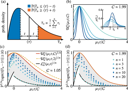
Figure 2: Non-asymptotic concentration and sample-size effects of empirical first-passage times $\overline{\tau}_{n}$ around the true mean $\langle\tau\rangle$. (a) Schematic probability density of $\overline{\tau}_{n}$ inferred from a (small) sample of $n$ realizations. Fluctuations are quantified by tail probabilities of deviations of $\overline{\tau}_{n}$ from $\langle\tau\rangle$ by more than $t$ towards the right $\mathbb{P}(\overline{\tau}_{n}\geq\langle\tau\rangle+t)$ or the left $\mathbb{P}(\overline{\tau}_{n}\leq\langle\tau\rangle-t)$ and are shown in orange and blue, respectively. (b) Dependence of the upper bounds $\mathcal{U}_{n}^{\pm}(\mu_{1}t;\mathcal{C})$ on sample size $n$ for the confined Brownian search in $d=3$. Bounds quantify how the probability of deviations from the sample mean drastically diminishes as $n$ increases (bright to dark; see (d)). Inset: corresponding empirical histogram of the sample mean $\overline{\tau}_{n}$ for different $n$ values. (c, d) Deviation probabilities and corresponding bounds for (c) a Markov network representation of protein folding ($\mathcal{C}\approx 1.05$) and (d) a spatially confined Brownian search ($\mathcal{C}\approx 1.99$) as introduced in Fig. 1. Probabilities are scaled as $\mathbb{P}^{1/n}({\rm sgn}(t)[\overline{\tau}_{n}-\langle\tau\rangle]\geq|t|)$; right tail areas are shown for $t>0$ and left for $t<0$, respectively. Lower $\mathcal{L}_{n}^{\pm}(\mu_{1}t)^{1/n}$ and upper bounds $\mathcal{U}_{n}^{\pm}(\mu_{1}t;\mathcal{C})^{1/n}$ are depicted as black and red lines, respectively, and the model-free bounds $\mathcal{U}_{n}^{\pm}(\mu_{1}t;2)^{1/n}$ are shown as yellow dashed line. Corresponding deviation probabilities obtained by numerical simulations as a function of $t$ for different fixed $n$ are denoted by symbols. Yellow and red curves coincide in (d) since $\mathcal{C}\approx 1.99$.

Here, we describe a solution of this problem in terms of the recently derived general upper bounds, so-called concentration inequalities, $\mathbb{P}(\pm[\overline{\tau}_{n}-\langle\tau\rangle]\geq t)\leq\mathcal{U}^{\pm}_{n}(t)$, which do not require the knowledge of the distribution of $\overline{\tau}_{n}$. Notably, these bounds are valid for all values $n\geq 1$ and $t\geq 0$ and their most conservative version is independent of any specific details about the underlying dynamics. From a technical perspective they are derived from a bounding technique referred to as the Cramér-Chernoff method boucheron2013concentration which is summarized briefly at the end of this section.

A complete derivation with all mathematical details is beyond the scope of this chapter (see bebon2023controlling ), we therefore only outline the key concepts. The procedure starts from Chernoff’s inequality $\mathbb{P}(\pm[\tau-\langle\tau\rangle]\geq t)\leq{\rm e}^{-\lambda t+\psi_{\pm(\tau-\langle\tau\rangle)}(\lambda)}$, where $\psi_{X}(\lambda)$ denotes the cumulant generating function of a random variable $X$ (see below), and essentially involves two main steps. First, we prove an upper bound on the cumulant generating function $\ln\langle\exp[\pm\lambda(\tau-\langle\tau\rangle)]\rangle\leq\phi_{\pm}(\lambda)$, $\lambda\in\mathbb{R}^{+}$, in the form of

$$\phi_{+}(\lambda)=\frac{\lambda^{2}}{2}\frac{\mu_{1}^{2}\langle\tau^{2}\rangle}{1-\lambda/\mu_{1}}\quad\text{and}\quad\phi_{-}(\lambda)=\frac{\lambda^{2}}{2}\frac{\mu_{1}^{2}\langle\tau^{2}\rangle}{1-(\lambda/\mu_{1})^{2}},$$ (9)

for the right tail ($\tau\geq\langle\tau\rangle$; index $+$) and left tail ($\tau<\langle\tau\rangle$; index $-$), respectively. In the second step we carry out a Legendre transform $\phi_{\pm}^{\ast}(t)\equiv\sup_{\lambda}[\lambda t-\phi_{\pm}(\lambda)]$ to optimize the bound. Considering the statistical independence of the $\tau_{i}$, the concentration bounds are found to have an exponential form $\mathbb{P}(\pm[\overline{\tau}_{n}-\langle\tau\rangle]\geq t)\leq\exp(-n\phi^{\ast}_{\pm}(t))$. Carrying out these steps we obtain the announced upper bounds bebon2023controlling

$$\mathbb{P}(\overline{\tau}_{n}-\langle\tau\rangle\geq t)\leq\exp(-n\mathcal{C}h_{+}(\mu_{1}t/\mathcal{C}))\equiv\mathcal{U}_{n}^{+}(\mu_{1}t;\mathcal{C})\quad 0\leq t\leq\infty$$

$$\mathbb{P}(\langle\tau\rangle-\overline{\tau}_{n}\geq t)\leq\exp(-n\mathcal{C}h_{-}(\mu_{1}t/\mathcal{C}))\equiv\mathcal{U}_{n}^{-}(\mu_{1}t;\mathcal{C})\quad 0\leq t\leq\langle\tau\rangle,$$ (10)

where we introduced $\mathcal{C}\equiv\mu_{1}^{2}\langle\tau^{2}\rangle$ and defined the auxiliary functions

$$h_{+}(u)\equiv 1+u-\sqrt{1+2u}\quad\text{and}\quad h_{-}(u)\equiv\Lambda(u)u-\frac{1}{2}\frac{\Lambda(u)^{2}}{1-\Lambda(u)^{2}},$$ (11)

with

$$\Lambda(u)\equiv\frac{1}{2}\left[g(u)-\sqrt{4+2/g(u)-g(u)^{2}}\right]$$ (12)

$$g(u)\equiv\frac{2}{\sqrt{3}}\left\{1+2\cosh\left[\frac{1}{3}\arccos\left(1+\frac{3^{3}}{2^{7}u^{2}}\right)\right]\right\}^{1/2}.$$ (13)

It is worth noting that, for the bounds presented in Eq. (10), the underlying details of the dynamics manifest solely via the system-dependent constant $\mathcal{C}$. Remarkably, however, it can be shown that for pseudo-equilibrium initial conditions ($x_{0}\sim\tilde{p}_{\rm eq}$; see end of Sec. 2.2) this constant falls within the range $0\leq\mathcal{C}\leq 2$ bebon2023controlling . This insight can be leveraged to directly establish

$$\mathcal{U}_{n}^{\pm}(\mu_{1}t;\mathcal{C})\leq\mathcal{U}_{n}^{\pm}(\mu_{1}t;2)\equiv\mathcal{U}_{n}^{\pm}(\mu_{1}t).$$ (14)

While these bounds tend to be more conservative (i.e., when the actual value of $\mathcal{C}$ significantly deviates from 2 one may still take $\mathcal{C}=2$ but the bound becomes less sharp), they are entirely model-independent. In the case of general initial conditions $p_{0}(x)\neq\tilde{p}_{\rm eq}$, $\mathcal{C}$ becomes replaced with a different constant (for details see bebon2023controlling ).

At this point we emphasize that the magnitude of deviations, in other words, the “error”, is naturally parameterized by the dimensionless variable $\mu_{1}t$ as evident from the argument of $h_{\pm}(\mu_{1}t/\mathcal{C})$ in Eq. (10). Therefore, considering errors in units $1/\mu_{1}$, $\pm\mu_{1}(\overline{\tau}_{n}-\langle\tau\rangle)$, there is no need to specify or know $\mu_{1}$ (i.e., the longest time-scale) itself. This relative error normalized by the “observable largest value” of first passage events $1/\mu_{1}$ thus quantifies the deviation of the inferred empirical mean first-passage time $\overline{\tau}_{n}$ from the true mean $\langle\tau\rangle$ relative to the characteristic (maximal, “extreme-case-scenario”) time-scale of the system. In this context deviation bounds (10) state that, for any sample size $n$, the probability $\mathbb{P}(\mu_{1}[\overline{\tau}_{n}-\langle\tau\rangle]\geq\mu_{1}t)$ of observing a relative error larger than a specified (dimensionless) value $\mu_{1}t$ (e.g., say $\mu_{1}t=0.1$ or 10%) is lower that the corresponding upper bound $\mathcal{U}_{n}^{\pm}(\mu_{1}t)$.

The validity of concentration bounds (10) and sample-size effects are illustrated in Fig. 2b-d for the target-search examples introduced earlier. To make the comparison, we evaluated “exact” empirical deviation probabilities (symbols) obtained from extensive sampling of $\overline{\tau}_{n}$ ($10^{11}$ repetitions) for various fixed values of $n$ (see inset Fig.2b for histograms of $\overline{\tau}_{n}$). For visualization purposes, we formally let $t\to-t$ for the left tails, allowing us to depict both, the right and left deviation bounds, in a single plot over the support $[-\langle\tau\rangle,\infty)$. Illustrated in Fig. 2b, deviation bounds quantify an exponential concentration rate of $\overline{\tau}_{n}$ around $\langle\tau\rangle$ as $n$ increases. In panels (c-d) we additionally employed the scaling $\mathbb{P}^{1/n}$ to collapse the results onto a single master curve for all values of $n$. Data points approach the upper bound as $n$ increases and as anticipated, the model-independent bound $\mathcal{U}_{n}^{\pm}(\mu_{1}t;2)$ (yellow) holds universally but tends to be more conservative.

Finally, we mention that in bebon2023controlling we also derived corresponding lower bounds $\mathcal{L}^{\pm}_{n}$, for the sake of completeness shown in black,

$$\mathbb{P}(\overline{\tau}_{n}-\langle\tau\rangle\geq t)\geq\left(w_{1}{\rm e}^{-\mu_{1}(\langle\tau\rangle+t)}\right)^{n}\equiv\mathcal{L}_{n}^{+}(\mu_{1}t)$$

$$\mathbb{P}(\langle\tau\rangle-\overline{\tau}_{n}\geq t)\geq\left(1-{\rm e}^{-\mu_{1}(\langle\tau\rangle-t)}\right)^{n}\equiv\mathcal{L}_{n}^{-}(\mu_{1}t),$$ (15)

by again leveraging the spectral analysis discussed in Sec. 2.2 in combination with ideas from extreme-value theory. Specifically, the searcher is assumed to start at $x_{0}$ drawn from pseudo-equilibrium $\tilde{p}_{\rm eq}(x)$. A detailed discussion of lower bounds (15)—explicitly demonstrating the existence of an intrinsic noise-floor—is beyond the scope of this chapter, as these do not play a role in the construction of performance guarantees presented in the following section. Nevertheless, these non-trivial lower bounds underscore the critical importance of a robust assessment of uncertainty of the observable $\overline{\tau}_{n}$, which we explore next.

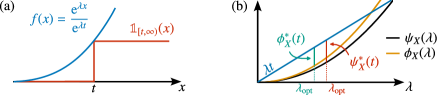
Figure 3: Sketch of the Cramér-Chernoff method. (a) Schematic of the inequality in Eq. (16). (b) Illustration of the Legendre transform of $\psi_{X}(\lambda)$ (black) and $\phi_{X}(\lambda)$ (yellow). The optimal $\lambda_{\rm opt}$ maximizes the difference with $\lambda t$ (blue); $\psi_{X}^{\ast}(t)$ (red) and $\phi_{X}^{\ast}(t)$ (green) denoting the corresponding Legendre transform (Eq. (18)), respectively. Note that $\phi_{X}(\lambda)\geq\psi_{X}(\lambda)$ implies $\phi_{X}^{\ast}(t)\leq\psi_{X}^{\ast}(t)$.

Cramér-Chernoff method in a nutshell Here we present a short overview of the Cramér-Chernoff method, for more details see, e.g., boucheron2013concentration . Consider a real-valued positive random variable $X$, in our context either $\tau-\langle\tau\rangle$ for the right tail or $\langle\tau\rangle-\tau$ for the left tail. For any $\lambda\in\mathbb{R}^{+}$, we begin with the obvious inequality (see Fig. 3a):

$$\vmathbb{1}_{[t,\infty)}\leq\frac{{\rm e}^{\lambda X}}{{\rm e}^{\lambda t}}\quad\forall X\geq 0,$$ (16)

where $\vmathbb{1}_{A}$ denotes the indicator function of set $A$. Taking expectation over $X$, $\langle\cdot\rangle$, on both sides, we immediately obtain

$$\mathbb{P}(X\geq t)\leq{\rm e}^{-\lambda t}\langle{\rm e}^{\lambda X}\rangle={\rm e}^{-\lambda t+\psi_{X}(\lambda)},$$ (17)

where $\psi_{X}(\lambda)\equiv\ln\langle{\rm e}^{\lambda X}\rangle$ denotes the cumulant generating function of $X$. Since this inequality holds for all values $\lambda\geq 0$, one can select $\lambda$ in a way that optimizes the upper bound, achieved by computing the Cramér-Legendre transform (see Fig. 3b)

$$\psi^{\ast}_{X}(t)=\sup_{\lambda\in\mathbb{R}^{+}}[\lambda t-\psi_{X}(\lambda)].$$ (18)

By Eq. (17) we thus obtain an upper bound on the tail probability according to

$$\mathbb{P}(X\geq t)\leq{\rm e}^{-\psi_{X}^{\ast}(t)}.$$ (19)

The strength of the method lies in its extension to sums $\overline{X}=X_{1}+\ldots+X_{n}$ of $n$ i.i.d. real-valued random variables $X_{1},\ldots X_{n}$. Due to independence, we have $\psi_{\overline{X}}(\lambda)=n\psi_{X}(\lambda)$, leading to $\psi^{\ast}_{\overline{X}}(t)=n\psi^{\ast}_{X}(t/n)$, in turn allowing one to write

$$\mathbb{P}(\overline{X}/n\geq t)\leq{\rm e}^{-n\psi^{\ast}_{X}(t)},$$ (20)

which underscores the evident connection to sample-averages like $\overline{\tau}_{n}$. We remark that in our case, the Legendre transform was computed not directly for $\psi_{X}(\lambda)$ but rather for $\phi_{X}(\lambda)\geq\psi_{X}(\lambda)$ (Eq. (9)), implying that $\psi_{X}^{\ast}(t)\geq\phi_{X}^{\ast}(t)$ (see Fig. 3b).

3.2 Uncertainty quantification

Having established the importance of assessing uncertainty in estimates derived from undersampled data, we are now confronted with the challenge of constructing reliable performance guarantees for the kinetic inference of empirical first-passage times $\overline{\tau}_{n}$. Unfortunately, for the task at hand many standard procedures fall short as they are grounded in asymptotic theory that necessitates a large sample size ($n\to\infty$). This requirement, clearly, is practically unattainable, making their applicability in sub-sampled regimes, by definition, problematic. Likewise, complementary approaches to statistical inference via Bayesian methods (see e.g., Ref. gelman1995bayesian ) face challenges when dealing with limited data, as the influence of prior distributions must be carefully considered. A sensitivity to the choice of a prior potentially results in “biased” prior-dependent uncertainty estimates, even in the large-sample limit.

This apparent lack of accurate finite-sample guarantees highlights the pressing need for reliable non-asymptotic error estimation techniques—e.g., in the form of confidence intervals—with correct finite-sample coverage probabilities to assess the quality of inferred estimates. Luckily, the concentration bounds (10) hold for any $n$, thus providing a well-suited candidate for addressing the challenges of the small-sample regime. As we will outline next, they provide a framework to quantify the discrepancy between the estimate $\overline{\tau}_{n}$ and the true parameter $\langle\tau\rangle$ in terms of non-asymptotic “with high probability” guarantees.

A construction of such performance guarantees is straightforward and easily implementable. By setting $\mathcal{U}_{n}^{\pm}(\mu_{1}t_{\alpha_{\pm},n}^{\pm})=\alpha_{\pm}$ for a user-defined acceptable left and right error probability of $\alpha_{\pm}$, we promptly obtain the implicit definition of a confidence interval $[-t_{\alpha_{-},n}^{-},t^{+}_{\alpha_{+},n}]$ in the form

$$\mathbb{P}(-t_{\alpha_{-},n}^{-}\leq\overline{\tau}_{n}-\langle\tau\rangle\leq t_{\alpha_{+},n}^{+})\geq 1-(\alpha_{-}+\alpha_{+})\equiv 1-\alpha$$ (21)

by performing an ordinary union bound. In other words, Eq. (21) asserts that with a high probability of at least $1-\alpha$ the inferred sample-average $\overline{\tau}_{n}$ falls within the interval $[\langle\tau\rangle-t_{\alpha_{-},n}^{-},\langle\tau\rangle+t_{\alpha_{+},n}^{+}]$ (see green region in Fig. 4a). For illustrative purposes we present in Fig. 4b the most conservative, universal $90\%$ confidence region (i.e., $\alpha=0.1$ and $\alpha_{\pm}=\alpha/2$) for the relative error as a function of the given sample-size $n$ for the model systems previously introduced in Secs. 2.3 and 2.4.

The non-asymptotic confidence intervals (21) are further valuable in addressing the equally important question of how large the minimal number of realizations $n_{\rm min}$ has to be if one wants to ensure that the error of the estimate $\overline{\tau}_{n_{\rm min}}$ does not exceed a specified threshold with a desired level of confidence—an essential consideration in the planning of experimental or computational studies. Correspondingly, this number is implicitly defined via

$$\mathcal{U}^{-}_{n_{\rm min}}(\mu_{1}t^{-}_{\alpha_{-},n};\mathcal{C})+\mathcal{U}^{+}_{n_{\rm min}}(\mu_{1}t^{+}_{\alpha_{+},n};\mathcal{C})=\alpha.$$ (22)

Using our simple examples, we explicitly show in Fig. 4c the minimal sample-size $n_{\rm min}$ necessary to guarantee a (dimensionless) relative error $\mu_{1}(\overline{\tau}_{n}-\langle\tau\rangle)$ of at most $\pm 10\%$ as a function of the confidence level $1-\alpha$ for the Markov network model (blue; $\mathcal{C}\approx 1.05$) and compare them with the most conservative model-independent version (black line). Note that the conservative bound holds for any setup that is described by Markovian dynamics as we introduced in Sec. 2.1 and a reliable inference of the mean (i.e., 90% confidence level; dashed line in Fig. 4c) typically requires hundreds to thousands of samples.

Collectively, Eqs. (21) and (22) provide a framework for evaluating uncertainties that arise in the kinetic inference of $\overline{\tau}_{n}$ when dealing with undersampled data. The required values of $t_{\alpha_{\pm},n}^{\pm}$ and $n_{\rm min}$ can readily be determined using standard root-finding techniques (e.g., bisection method). We remark that in our discussion, we have chosen equal tail probabilities $\alpha_{\pm}=\alpha/2$, resulting in what are commonly referred to as “central” confidence intervals. However, in general, two-sided confidence regions are not uniquely defined by their confidence level, and various other choices exist (e.g., symmetric intervals). Expanding on this, there are situations where only one-sided confidence intervals are needed bebon2023controlling . In this case we even explicitly obtain that

$$\overline{\tau}_{n}-\langle\tau\rangle\leq-\frac{\ln(\alpha)}{\mu_{1}n}+\frac{\sqrt{2}\sqrt{-\ln(\alpha)}}{\mu_{1}\sqrt{n/\mathcal{C}}}$$ (23)

with probability of $1-\alpha$. Correspondingly, one obtains the explicit bound

$$n_{\rm min}^{\pm}\geq-\frac{\ln(\alpha_{\pm})}{\mathcal{C}h_{\pm}(\mu_{1}t/\mathcal{C})}$$ (24)

where $n_{\rm min}^{\pm}$ now denotes the required sample-sizes to ensure that $\pm(\overline{\tau}_{n}-\langle\tau\rangle)\leq t$ with a probability of at least $1-\alpha_{\pm}$.

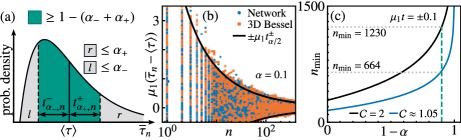
Figure 4: Uncertainty quantification of the sample-mean $\overline{\tau}_{n}$ for any sample-size $n$. (a) Probability that the sample-mean $\overline{\tau}_{n}$ lies within an interval of $[-t_{\alpha_{-},n}^{-},t_{\alpha_{+},n}^{+}]$ around $\langle\tau\rangle$ with a probability of at least $1-(\alpha_{-}+\alpha_{+})$. (b) Model-free 90% confidence region (i.e., $\alpha=0.1$) that the error in units $1/\mu_{1}$ remains within $\pm 10\%$ as a function of sample-size $n$. (c) Minimal-sample size $n_{\rm min}$ required to ensure that the relative error $\mu_{1}(\overline{\tau}_{n}-\langle\tau\rangle)$ does not exceed $\pm 10\%$ as a function of confidence level $1-\alpha$; a confidence of at least $90\%$ is shown as dashed line.

4 Going beyond the mean first-passage time

Thus far we reviewed recent advances in quantifying uncertainty of the sample-mean $\overline{\tau}_{n}$ inferred from a (small) finite number $n$ of experimental or simulated trajectories, and explored how many samples are needed to ensure that the uncertainty of $\overline{\tau}_{n}$ falls below a predefined threshold value. However, the fact that possibly multiple relevant time-scales are at play (e.g., in “compact” search processes Olivier_NC ; Bnichou2014 ; Godec_PRX ; Godec_SciRep ) introduces an additional layer of complexity to the uncertainty of $\overline{\tau}_{n}$. In such situations the mean on its own may not be a sufficient statistic (i.e., as the “characteristic” time-scale) and a priori may not faithfully characterize the entire distribution. This calls for a deeper understanding of the first-passage time density $\wp_{a}(t)$, including aspects such as its behavior in the short and long-time regimes Grebenkov_2018_2 ; Olivier_NC ; Bnichou2014 ; Godec_PRX ; Godec_SciRep .

Interestingly, assuming that a reliable estimate of the mean is available (which can be achieved using the outlined procedure designed to handle uncertainty in $\overline{\tau}_{n}$ even where estimation becomes challenging, including scenarios involving multiple time-scales), we can apply the upper bounds $\mathcal{U}_{n}^{\pm}(t)$ to gain insight. By inspecting the case $n=1$, i.e., $\overline{\tau}_{n}=\tau$ and $\mathbb{P}(\pm[\tau-\langle\tau\rangle]\geq t)\leq\mathcal{U}^{\pm}(t)$, the bounds directly provide knowledge about the tail regions of the first-passage time density $\wp_{a}(t)$ (see Fig. 2a) since, in this scenario, the mean first-passage time $\langle\tau\rangle$ acts as a “reference point”. Understanding these tail regions is crucial, as trajectories that survive for long times (right tail) explore their environment extensively, and thus retain information about structural properties. Conversely, shorter trajectories (left tail) typically reach their target more directly, often following the shortest direct path and reveal intricate features such as the number of energy minima Tolya . On top of that, in cases where the mean is not a priori representative the spread of extreme (i.e., minimal and maximal) first-passage times provides insight about the range of first-passage events (see below).

Another intriguing and related challenge emerges when moving beyond the “single searcher setting” to the first-passage properties of multiple searchers — the fastest search time Hartich_2018 ; Hartich_Book ; Lawley_1 ; Lawley_2 ; Lawley_3 . Here, the statistics may be dominated by the time it takes the fastest (minimal $\tau$) or slowest (maximal $\tau$) out of many searchers to reach a target for the first time. This phenomenon is particularly evident in various biological systems, such as the search process of sperm cells seeking an egg cell Yang2015 .

Motivated by these challenges, we now summarize recent progress in understanding first-passage properties in scenarios where the mean first-passage time $\langle\tau\rangle$ alone falls short in capturing the complete range of the dynamics or when dealing with multiple searchers bebon2023controlling .

4.1 Bounding extreme deviations

The presence of many different distinct time-scales is already included in the spectral expansion of the first-passage time density $\wp_{a}(t)=\sum_{k}w_{k}^{\rm eq}\mu_{k}\exp(-\mu_{k}t)$; recall that $w_{k}^{\rm eq}\geq 0,\forall k$ for pseudo-equilibrium initial conditions. Evidently, whenever more than a single weight $w_{k}^{\rm eq}$ contributes, multiple time-scales become relevant. In such cases, relying solely on the knowledge of $\langle\tau\rangle$ may not suffice for an accurate characterization of the entire dynamics, as $\wp_{a}(t)$ significantly deviates from a single exponential. For the following discussion we will make use of the fact that the presence of multiple time-scales is reflected in the dimensionless factor $\mu_{1}\langle\tau\rangle\in(0,1]$, i.e., it substantially differs from 1, and the dimensionless parameter $\mathcal{C}=\mu_{1}^{2}\langle\tau^{2}\rangle$ becomes substantially smaller than 2.

To address the range of these sample-to-sample fluctuations of the first-passage time $\tau$ we consider extreme deviations from the mean, i.e., we are interested how much the maximal $\tau^{+}_{n}\equiv\max_{i\in[1,n]}\tau_{i}$ and minimal $\tau_{n}^{-}\equiv\min_{i\in[1,n]}\tau_{i}$ in a sample of $n$ i.i.d. observed first-passage times $\tau_{i}$ deviate from the mean (see Fig. 5a) on average. This expected range of extreme deviations $\langle m_{n}^{\pm}\rangle\equiv\langle\tau_{n}^{\pm}-\langle\tau\rangle\rangle$ is the appropriate observable controlling uncertainty when multiple time-scales are concerned, especially in the small-sample setting, as it provides information regarding the spread (i.e., uncertainty) of observations. To this end, we recently derived sharp two-sided “squeeze” bounds bebon2023controlling

$$\underline{\mathcal{M}}_{n}^{\pm}\leq\langle m_{n}^{\pm}\rangle\leq\overline{\mathcal{M}}_{n}^{\pm},\quad n\geq 1$$ (25)

in the form of

$$\overline{\mathcal{M}}_{n}^{+}\equiv\sum_{k=1}^{n}\binom{n}{k}(-1)^{k+1}\frac{(\mu_{1}\langle\tau\rangle)^{k}}{\mu_{1}k}-\langle\tau\rangle, \overline{\mathcal{M}}_{n}^{-}\equiv\langle\tau\rangle\left[\frac{1}{n}-1\right]$$

$$\underline{\mathcal{M}}_{n}^{+}\equiv\langle\tau\rangle\sum_{k=2}^{n}\frac{1}{k}, \underline{\mathcal{M}}_{n}^{-}\equiv\langle\tau\rangle\left[\frac{1}{n}(\mu_{1}\langle\tau\rangle)^{n-1}-1\right].$$ (26)

Notably, in dimensionless units of $1/\mu_{1}$, these bounds are functions of $\mu_{1}\langle\tau\rangle$ only. In other words, the mean $\langle\tau\rangle$ sharply bounds the expected range of extreme first-passage times even when it is a priori not a representative statistic due to the presence of multiple time-scales. Therefore, these results motivate an estimation of $\langle\tau\rangle$ via $\overline{\tau}_{n}$ even in the presence of many time-scales. The validity and sharpness is depicted in Fig. 5b,c for expected deviations of the maximum (blue) and the minimum (orange) for the Markov jump network from Fig. 1c. Each data point corresponds to one particular realization of the jump process (see Sec. 2.3) where transition rates are drawn randomly under the constraint of detailed balance. Note that the “squeeze” bounds (26) can be saturated (for a discussion see bebon2023controlling ).

Figure 5: Extreme deviations from the mean first-passage time. (a) Maximal $\tau_{n}^{+}\equiv\max_{i\in[1,n]}\tau_{i}$ and minimal $\tau_{n}^{-}\equiv\min_{i\in[1,n]}\tau_{i}$ first-passage time in a sample of $n$ i.i.d. realizations. (b, c) Average maximal ($+$) and minimal ($-$) deviation from the mean $\langle m_{n}^{\pm}\rangle\equiv\langle\tau_{n}^{\pm}-\langle\tau\rangle\rangle$ from extensive computer simulations (symbols) with lower $\underline{\mathcal{M}}_{n}^{\pm}$ (dashed black lines) and upper $\overline{\mathcal{M}}_{n}^{\pm}$ bound (black lines) shown for $n=10$ and $n=3$, respectively. Quantities are expressed in units of $1/\mu_{1}$ and shown as a function of $\mu_{1}\langle\tau\rangle$.

Considering that the maximal and minimal first-passage time in a sample of $n$ i.i.d. realizations can be viewed as representing the fastest and slowest first-passage times among the $n$ independent searchers, respectively, these results provide insight into the slowest and fastest first-passage events of $n$ independent searchers. Therefore, it is anticipated that these bounds will prove to be relevant in target-searches with multiple searches and in the few-encounter limit.

5 Discussion

To robustly asses the uncertainty of inferred empirical first-passage times in the small-sample regime in a general setting, one needs to go beyond conventional approaches relying on asymptotic reasoning or require prior belief. In this chapter, we presented one approach that achieves reliable error estimates by tackling the issue from a non-asymptotic concentration-of-measure perspective that builds on spectral properties of the first-passage problem.

In particular, we put forward a framework that allows to bound uncertainties associated with empirical first-passage times in terms of deviation probabilities that hold regardless of sample size. Subsequently, we showcased how these bounds can be applied by constructing non-asymptotic confidence intervals, which allowed us to tackle the critical question of what sample size is required to ensure tolerable errors.

In the last part, we addressed the challenging situation of many relevant time-scales, where it is no longer adequate to rely solely on the mean first-passage time for an appropriate description. In doing so, we presented sharp non-asymptotic bounds on average minimal and maximal deviations around the mean, and argued that these results have direct implications for target-search processes with multiple searchers.

To conclude, the presented framework of non-asymptotic uncertainty quantification is applicable to the broad class of reversible Markov dynamics that include discrete Markovian jump-processes in any dimension and Markovian diffusion in effectively one-dimensional potential landscapes. Accordingly, it will be interesting to see how the developed theory can be turned into new statistical tests in the future. Moreover, extensions to, for example, irreversible (i.e., driven) dynamics and more complicated observables will be carried out in the future.

- (1) S. Redner, A Guide to First-Passage Processes (Cambridge University Press, Cambridge, 2001).
- (2) R. Metzler, S. Redner, and G. Oshanin, First-Passage Phenomena and their Applications (World Scientific, Singapore, 2014).
- (3) K. Lindenberg, R. Metzler, and G. Oshanin, Chemical Kinetics: Beyond the Textbook (World Scientific, New Jersey, 2019).
- (4) S. Iyer-Biswas and A. Zilman, First-passage processes in cellular biology, Adv. Chem. Phys. 160, 261–306 (2016).
- (5) Y. Zhang and O. K. Dudko, First-passage processes in the genome, Annu. Rev. Biophys. 45, 117–134 (2016).
- (6) H. Kramers, Brownian motion in a field of force and the diffusion model of chemical reactions, Physica 7, 284 – 304 (1940).
- (7) P. Hänggi, P. Talkner, and M. Borkovec, Reaction-rate theory: fifty years after kramers, Rev. Mod. Phys. 62, 251–341 (1990).
- (8) A. Szabo, K. Schulten, and Z. Schulten, First passage time approach to diffusion controlled reactions, J. Chem. Phys. 72, 4350–4357 (1980).
- (9) E. Ben-Naim, S. Redner, and F. Leyvraz, Decay kinetics of ballistic annihilation, Phys. Rev. Lett. 70, 1890–1893 (1993).
- (10) D. S. Grebenkov, R. Metzler, and G. Oshanin, Towards a full quantitative description of single-molecule reaction kinetics in biological cells, Phys. Chem. Chem. Phys. 20, 16393–16401 (2018).
- (11) D. S. Grebenkov, R. Metzler, and G. Oshanin, Strong defocusing of molecular reaction times results from an interplay of geometry and reaction control, Commun. Chem. 1, 1 (2018).
- (12) D. S. Grebenkov, Universal formula for the mean first passage time in planar domains, Phys. Rev. Lett. 117, 260201 (2016).
- (13) P. C. Bressloff and J. M. Newby, Stochastic models of intracellular transport, Rev. Mod. Phys. 85, 135–196 (2013).
- (14) É. Roldán, A. Lisica, D. Sánchez-Taltavull, and S. W. Grill, Stochastic resetting in backtrack recovery by RNA polymerases, Phys. Rev. E 93, 062411 (2016).
- (15) K. R. Ghusinga, J. J. Dennehy, and A. Singh, First-passage time approach to controlling noise in the timing of intracellular events, Proc. Natl. Acad. Sci. 114, 693–698 (2017).
- (16) K. Rijal, A. Prasad, A. Singh, and D. Das, Exact distribution of threshold crossing times for protein concentrations: Implication for biological timekeeping, Phys. Rev. Lett. 128, 048101 (2022).
- (17) J. J. Parmar, D. Das, and R. Padinhateeri, Theoretical estimates of exposure timescales of protein binding sites on DNA regulated by nucleosome kinetics, Nucleic Acids Res. 44, 1630–1641 (2015).
- (18) D. A. Charlebois, N. Abdennur, and M. Kaern, Gene expression noise facilitates adaptation and drug resistance independently of mutation, Phys. Rev. Lett. 107, 218101 (2011).
- (19) F. Frey, F. Ziebert, and U. S. Schwarz, Stochastic dynamics of nanoparticle and virus uptake, Phys. Rev. Lett. 122, 088102 (2019).
- (20) A. L. Lloyd and R. M. May, How viruses spread among computers and people, Science 292, 1316–1317 (2001).
- (21) L. Hufnagel, D. Brockmann, and T. Geisel, Forecast and control of epidemics in a globalized world, Proc. Natl. Acad. Sci. 101, 15124–15129 (2004).
- (22) O. Bénichou, C. Loverdo, M. Moreau, and R. Voituriez, Intermittent search strategies, Rev. Mod. Phys. 83, 81–129 (2011).
- (23) F. Boccardo and O. Pierre-Louis, Controlling the shape of small clusters with and without macroscopic fields, Phys. Rev. Lett. 128, 256102 (2022).
- (24) T. Erdmann and U. S. Schwarz, Stability of adhesion clusters under constant force, Phys. Rev. Lett. 92, 108102 (2004).
- (25) S. Chakrabarti, M. Hinczewski, and D. Thirumalai, Plasticity of hydrogen bond networks regulates mechanochemistry of cell adhesion complexes, Proc. Natl. Acad. Sci. 111, 9048–9053 (2014).
- (26) K. Blom and A. Godec, Criticality in cell adhesion, Phys. Rev. X 11, 031067 (2021).
- (27) I. Goychuk and P. Hänggi, Ion channel gating: A first-passage time analysis of the kramers type, Proc. Natl. Acad. Sci. 99, 3552–3556 (2002).
- (28) O. G. Berg, R. B. Winter, and P. H. Von Hippel, Diffusion-driven mechanisms of protein translocation on nucleic acids. 1. models and theory, Biochem. 20, 6929–6948 (1981).
- (29) E. Koslover, M. Díaz de la Rosa, and A. Spakowitz, Theoretical and computational modeling of target-site search kinetics in vitro and in vivo, Biophys. J. 101, 856 – 865 (2011).
- (30) D. Holcman and Z. Schuss, Time scale of diffusion in molecular and cellular biology, J. Phys. A: Math. Theor. 47, 173001 (2014).
- (31) O. Bénichou, C. Chevalier, B. Meyer, and R. Voituriez, Facilitated diffusion of proteins on chromatin, Phys. Rev. Lett. 106, 038102 (2011).
- (32) E. G. Marklund, A. Mahmutovic, O. G. Berg, P. Hammar, D. van der Spoel, D. Fange, and J. Elf, Transcription-factor binding and sliding on dna studied using micro- and macroscopic models, Proc. Natl. Acad. Sci. 110, 19796–19801 (2013).
- (33) M. Bauer and R. Metzler, In vivo facilitated diffusion model, PLoS ONE 8, e53956 (2013).
- (34) O. Bénichou, C. Chevalier, J. Klafter, B. Meyer, and R. Voituriez, Geometry-controlled kinetics, Nat. Chem. 2, 472–477 (2010).
- (35) O. Bénichou and R. Voituriez, From first-passage times of random walks in confinement to geometry-controlled kinetics, Phys. Rep. 539, 225–284 (2014).
- (36) A. Godec and R. Metzler, Universal proximity effect in target search kinetics in the few-encounter limit, Phys. Rev. X 6, 041037 (2016).
- (37) A. F.Siegert, On the first passage time probability problem, Phys. Rev E 81, 617–623 (1951).
- (38) J. Newby and J. Allard, First-passage time to clear the way for receptor-ligand binding in a crowded environment, Phys. Rev. Lett. 116, 128101 (2016).
- (39) I. Nayak, D. Das, and A. Nandi, Comparison of mechanisms of kinetochore capture with varying number of spindle microtubules, Phys. Rev. Res. 2, 013114 (2020).
- (40) Z. Schuss, Theory and Applications of Stochastic Processes: An Analytical Approach (Springer Science & Business Media, New York, 2009).
- (41) J.-P. Bouchaud and M. Potters, Theory of Financial Risk and Derivative Pricing: From Statistical Physics to Risk Management (Cambridge University Press, Cambridge, 2003).
- (42) W. Paul and J. Baschnagel, Stochastic Processes: From Physics to Finance (Springer International Publishing, Cham, 2013).
- (43) C. W. Gardiner, Handbook of Stochastic Methods for Physics, Chemistry and the Natural Sciences (Springer, Berlin, 1985).
- (44) D. B. Dougherty, I. Lyubinetsky, E. D. Williams, M. Constantin, C. Dasgupta, and S. Sarma, Experimental persistence probability for fluctuating steps, Phys. Rev. Lett. 89, 136102 (2002).
- (45) M. Constantin, S. D. Sarma, C. Dasgupta, O. Bondarchuk, D. B. Dougherty, and E. D. Williams, Infinite family of persistence exponents for interface fluctuations, Phys. Rev. Lett. 91, 086103 (2003).
- (46) J. Merikoski, J. Maunuksela, M. Myllys, J. Timonen, and M. J. Alava, Temporal and spatial persistence of combustion fronts in paper, Phys. Rev. Lett. 90, 024501 (2003).
- (47) M. Constantin, C. Dasgupta, P. P. Chatraphorn, S. N. Majumdar, and S. D. Sarma, Persistence in nonequilibrium surface growth, Phys. Rev. E 69, 061608 (2004).
- (48) D. B. Dougherty, C. Tao, O. Bondarchuk, W. G. Cullen, E. D. Williams, M. Constantin, C. Dasgupta, and S. D. Sarma, Sampling-time effects for persistence and survival in step structural fluctuations, Phys. Rev. E 71, 021602 (2005).
- (49) C. Godrèche, S. N. Majumdar, and G. Schehr, Longest excursion of stochastic processes in nonequilibrium systems, Phys. Rev. Lett. 102, 240602 (2009).
- (50) A. J. Bray, S. N. Majumdar, and G. Schehr, Persistence and first-passage properties in nonequilibrium systems, Adv. Phys. 62, 225–361 (2013).
- (51) T. Kay and L. Giuggioli, Diffusion through permeable interfaces: Fundamental equations and their application to first-passage and local time statistics, Phys. Rev. Res. 4, 032039 (2022).
- (52) S. Bo, L. Hubatsch, J. Bauermann, C. A. Weber, and F. Jülicher, Stochastic dynamics of single molecules across phase boundaries, Phys. Rev. Res. 3, 043150 (2021).
- (53) U. Seifert, Stochastic thermodynamics, fluctuation theorems and molecular machines, Rep. Prog. Phys. 75, 126001 (2012).
- (54) T. R. Gingrich and J. M. Horowitz, Fundamental bounds on first passage time fluctuations for currents, Phys. Rev. Lett. 119, 170601 (2017).
- (55) S. Singh, P. Menczel, D. S. Golubev, I. M. Khaymovich, J. T. Peltonen, C. Flindt, K. Saito, É. Roldán, and J. P. Pekola, Universal first-passage-time distribution of non-gaussian currents, Phys. Rev. Lett. 122, 230602 (2019).
- (56) E. Roldán, I. Neri, M. Dörpinghaus, H. Meyr, and F. Jülicher, Decision making in the arrow of time, Phys. Rev. Lett. 115, 250602 (2015).
- (57) I. Neri, E. Roldán, and F. Jülicher, Statistics of infima and stopping times of entropy production and applications to active molecular processes, Phys. Rev. X 7, 011019 (2017).
- (58) G. Falasco and M. Esposito, Dissipation-time uncertainty relation, Phys. Rev. Lett. 125, 120604 (2020).
- (59) I. Neri, Estimating entropy production rates with first-passage processes, J. Phys. A: Math. Theor. 55, 304005 (2022).
- (60) J. P. Garrahan, Simple bounds on fluctuations and uncertainty relations for first-passage times of counting observables, Phys. Rev. E 95, 032134 (2017).
- (61) K. Hiura and S. ichi Sasa, Kinetic uncertainty relation on first-passage time for accumulated current, Phys. Rev. E 103, 050103 (2021).
- (62) M. Kac, On some connections between probability theory and differential and integral equations, Proceedings of the Second Berkeley Symposium on Mathematical Statistics and Probability, pp. 189–215, (University of California Press, Berkeley, 1951). D. Hartich and A. Godec, Reaction Kinetics in the Few-Encounter Limit, in Chemical Kinetics (World Scientific, New Jersey, 2019), chap. 11, pp. 265–283.
- (63) G. Schehr and S. N. Majumdar, Exact record and order statistics of random walks via first-passage ideas, in First-Passage Phenomena and Their Applications (World Scientific, Singapore, 2014), chap. 1, pp. 226–251.
- (64) S. N. Majumdar, G. Schehr, and G. Wergen, Record statistics and persistence for a random walk with a drift, J. Phys. A: Math. Theor. 45, 355002 (2012).
- (65) D. Hartich and A. Godec, Extreme value statistics of ergodic markov processes from first passage times in the large deviation limit, J. Phys. A: Math. Theor. 52, 244001 (2019).
- (66) H. Friedman, D. A. Kessler, and E. Barkai, Quantum walks: The first detected passage time problem, Phys. Rev. E 95, 032141 (2017).
- (67) F. Thiel, E. Barkai, and D. A. Kessler, First detected arrival of a quantum walker on an infinite line, Phys. Rev. Lett. 120, 040502 (2018).
- (68) M. J. Kearney and S. N. Majumdar, On the area under a continuous time brownian motion till its first-passage time, J. Phys. A: Math. Gen. 38, 4097–4104 (2005).
- (69) M. J. Kearney, S. N. Majumdar, and R. J. Martin, The first-passage area for drifted brownian motion and the moments of the airy distribution, J. Phys. A: Math. Theor. 40, F863–F869 (2007).
- (70) M. J. Kearney and S. N. Majumdar, Statistics of the first passage time of brownian motion conditioned by maximum value or area, J. Phys. A: Math. Theor. 47, 465001 (2014).
- (71) M. J. Kearney and R. J. Martin, Statistics of the first passage area functional for an ornstein–uhlenbeck process, J. Phys. A: Math. Theor. 54, 055002 (2021).
- (72) S. N. Majumdar and B. Meerson, Statistics of first-passage brownian functionals, J. Stat. Mech.: Theory Exp., 023202 (2020).
- (73) P. Singh and A. Pal, First-passage brownian functionals with stochastic resetting, J. Phys. A: Math. Theor. 55, 234001 (2022).
- (74) G. Mercado-Vásquez and D. Boyer, First hitting times to intermittent targets, Phys. Rev. Lett. 123, 250603 (2019).
- (75) A. Kumar, A. Zodage, and M. S. Santhanam, First detection of threshold crossing events under intermittent sensing, Phys. Rev. E 104, 052103 (2021).
- (76) J. L. Spouge, A. Szabo, and G. H. Weiss, Single-particle survival in gated trapping, Phys. Rev. E 54, 2248–2255 (1996).
- (77) Y. Scher and S. Reuveni, Unified approach to gated reactions on networks, Phys. Rev. Lett. 127, 018301 (2021).
- (78) A. Kumar, Y. Scher, S. Reuveni, and M. S. Santhanam, Inference from gated first-passage times, Phys. Rev. Res. 5 (2023).
- (79) E. Woillez, Y. Zhao, Y. Kafri, V. Lecomte, and J. Tailleur, Activated escape of a self-propelled particle from a metastable state, Phys. Rev. Lett. 122, 258001 (2019).
- (80) F. Mori, P. L. Doussal, S. N. Majumdar, and G. Schehr, Universal survival probability for a -dimensional run-and-tumble particle, Phys. Rev. Lett. 124, 090603 (2020).
- (81) F. D. Trapani, T. Franosch, and M. Caraglio, Active brownian particles in a circular disk with an absorbing boundary, Phys. Rev. E 107 (2023).
- (82) P. Hänggi and P. Talkner, Memory index of first-passage time: A simple measure of non-markovian character, Phys. Rev. Lett. 51, 2242–2245 (1983).
- (83) P. Hanggi and P. Talkner, First-passage time problems for non-markovian processes, Phys. Rev. A 32, 1934–1937 (1985).
- (84) T. Guérin, N. Levernier, O. Bénichou, and R. Voituriez, Mean first-passage times of non-markovian random walkers in confinement, Nature 534, 356–359 (2016).
- (85) M. R. Evans and S. N. Majumdar, Diffusion with stochastic resetting, Phys. Rev. Lett. 106, 160601 (2011).
- (86) L. Kusmierz, S. N. Majumdar, S. Sabhapandit, and G. Schehr, First order transition for the optimal search time of lévy flights with resetting, Phys. Rev. Lett. 113, 220602 (2014).
- (87) S. Reuveni, Optimal stochastic restart renders fluctuations in first passage times universal, Phys. Rev. Lett. 116, 170601 (2016).
- (88) A. Pal and S. Reuveni, First passage under restart, Phys. Rev. Lett. 118, 030603 (2017).
- (89) A. Pal, I. Eliazar, and S. Reuveni, First passage under restart with branching, Phys. Rev. Lett. 122, 020602 (2019).
- (90) M. R. Evans, S. N. Majumdar, and G. Schehr, Stochastic resetting and applications, J. Phys. A: Math. Theor. 53, 193001 (2020).
- (91) B. Besga, A. Bovon, A. Petrosyan, S. N. Majumdar, and S. Ciliberto, Optimal mean first-passage time for a brownian searcher subjected to resetting: Experimental and theoretical results, Phys. Rev. Res. 2, 032029 (2020).
- (92) O. Tal-Friedman, A. Pal, A. Sekhon, S. Reuveni, and Y. Roichman, Experimental realization of diffusion with stochastic resetting, J. Phys. Chem. Lett. 11, 7350–7355 (2020).
- (93) B. D. Bruyne, J. Randon-Furling, and S. Redner, Optimization in first-passage resetting, Phys. Rev. Lett. 125, 050602 (2020).
- (94) B. D. Bruyne, S. N. Majumdar, and G. Schehr, Optimal resetting brownian bridges via enhanced fluctuations, Phys. Rev. Lett. 128, 200603 (2022).
- (95) V. Stojkoski, P. Jolakoski, A. Pal, T. Sandev, L. Kocarev and R. Metzler, Income inequality and mobility in geometric Brownian motion with stochastic resetting: theoretical results and empirical evidence of non-ergodicity, Phil. Trans. R. Soc. A. 380, 20210157 (2022).
- (96) P. Xu, T. Zhou, R. Metzler, W. Deng, Stochastic harmonic trapping of Lévy walk: transport and first-passage dynamics under soft resetting strategies, New J. Phys. 24, 033003 (2022).
- (97) D. Hartich and A. Godec, Duality between relaxation and first passage in reversible markov dynamics: rugged energy landscapes disentangled, New J. Phys. 20, 112002 (2018).
- (98) D. Hartich and A. Godec, Interlacing relaxation and first-passage phenomena in reversible discrete and continuous space markovian dynamics, J. Stat. Mech. 2019, 024002 (2019).
- (99) R. Bebon and A. Godec, Controlling uncertainty of empirical first-passage times in the small-sample regime, Phys. Rev. Lett. 131, 237101 (2023).
- (100) A. V. Skorokhod, Stochastic equations for diffusion processes in a bounded region, Theory Probab. its Appl. 6, 264–274 (1961).
- (101) K. Ito and H. P. McKean, Diffusion Processes and Their Sample Paths, (Springer-Verlag, Berlin, 1965).
- (102) H. Tanaka, Stochastic differential equations with reflecting boundary condition in convex regions, Hiroshima Math. J. 9, 163–177 (1979).
- (103) P.-L. Lions and A.-S. Sznitman, Stochastic differential equations with reflecting boundary conditions, Commun. Pure Appl. Math. 37, 511–537 (1984).
- (104) D. S. Grebenkov, Probability distribution of the boundary local time of reflected Brownian motion in Euclidean domains, Phys. Rev. E 100, 062110 (2019).
- (105) D. S. Grebenkov, Paradigm shift in diffusion-mediated surface phenomena, Phys. Rev. Lett. 125, 078102 (2020).
- (106) T. G. Mattos, C. Mejía-Monasterio, R. Metzler, and G. Oshanin, First passages in bounded domains: When is the mean first passage time meaningful?, Phys. Rev. E 86, 031143 (2012).
- (107) C. Chevalier, O. Bénichou, B. Meyer, and R. Voituriez, First-passage quantities of brownian motion in a bounded domain with multiple targets: a unified approach, J. Phys. A: Math. Theor. 44, 025002 (2010).
- (108) B. Meyer, C. Chevalier, R. Voituriez, and O. Bénichou, Universality classes of first-passage-time distribution in confined media, Phys. Rev. E 83, 051116 (2011).
- (109) G. R. Bowman, V. S. Pande, and F. Noé, An Introduction to Markov State Models and their Application to Long Timescale Molecular Simulation (Springer Science & Business Media, Dordrecht, 2013).
- (110) F. Noé, S. Olsson, J. Köhler, and H. Wu, Boltzmann generators: Sampling equilibrium states of many-body systems with deep learning, Science 365 (2019).
- (111) E. Braun, J. Gilmer, H. B. Mayes, D. L. Mobley, J. I. Monroe, S. Prasad, and D. M. Zuckerman, Best practices for foundations in molecular simulations [article v1.0], Living J. Comp. Mol. Sci. 1, 1 (2019).
- (112) R. V. Hogg, J. W. McKean, and A. T. Craig, Introduction to Mathematical Statistics (Pearson, Boston, 2018).
- (113) K. Lindorff-Larsen, S. Piana, R. O. Dror, and D. E. Shaw, How fast-folding proteins fold, Science 334, 517–520 (2011).
- (114) J. L. Adelman and M. Grabe, Simulating rare events using a weighted ensemble-based string method, J. Chem. Phys. 138, 044105 (2013).
- (115) V. Gapsys and B. L. de Groot, On the importance of statistics in molecular simulations for thermodynamics, kinetics and simulation box size, eLife 9, e57589 (2020).
- (116) B. Mostofian and D. M. Zuckerman, Statistical uncertainty analysis for small-sample, high log-variance data: Cautions for bootstrapping and bayesian bootstrapping, J. Chem. Theory Comput. 15, 3499–3509 (2019).
- (117) R. Mehra and K. P. Kepp, Cell size effects in the molecular dynamics of the intrinsically disordered a peptide, J. Chem. Phys. 151, 085101 (2019).
- (118) A. Militaru, M. Innerbichler, M. Frimmer, F. Tebbenjohanns, L. Novotny, and C. Dellago, Escape dynamics of active particles in multistable potentials, Nat. Commun. 12, 1 (2021).
- (119) L. Rondin, J. Gieseler, F. Ricci, R. Quidant, C. Dellago, and L. Novotny, Direct measurement of kramers turnover with a levitated nanoparticle, Nat. Nanotechnol. 12, 1130–1133 (2017).
- (120) O. Pulkkinen, R. Metzler, Variance-corrected Michaelis-Menten equation predicts transient rates of single-enzyme reactions and response times in bacterial gene-regulation, Sci. Rep. 5, 17820 (2015).
- (121) S. Boucheron, G. Lugosi, and P. Massart, Concentration Inequalities: A Nonasymptotic Theory of Independence (Oxford University Press, New York, 2013).
- (122) A. Gelman, J. B. Carlin, H. S. Stern, and D. B. Rubin, Bayesian Data Analysis (Chapman and Hall/CRC, London, 1995).
- (123) A. Godec and R. Metzler, First passage time distribution in heterogeneity controlled kinetics: going beyond the mean first passage time, Sci. Rep. 6 (2016).
- (124) A. L. Thorneywork, J. Gladrow, Y. Qing, M. Rico-Pasto, F. Ritort, H. Bayley, A. B. Kolomeisky, and U. F. Keyser, Direct detection of molecular intermediates from first-passage times, Sci. Adv. 6, 1 (2020).
- (125) D. Hartich and A. Godec, Reaction Kinetics in the Few-Encounter Limit, in Chemical Kinetics (World Scientific, New Jersey, 2019), chap. 11, pp. 265–283.
- (126) S. D. Lawley and J. B. Madrid, First passage time distribution of multiple impatient particles with reversible binding, J. Chem. Phys. 150, 214113 (2019).
- (127) S. D. Lawley and J. B. Madrid, A probabilistic approach to extreme statistics of brownian escape times in dimensions 1, 2, and 3, J. Nonlin. Sci. 30, 1207–1227 (2020).
- (128) S. D. Lawley, Universal formula for extreme first passage statistics of diffusion, Phys. Rev. E 101, 012413 (2020).
- (129) J. Yang, I. Kupka, Z. Schuss, and D. Holcman, Search for a small egg by spermatozoa in restricted geometries, J. Math. Biol. 73, 423–446 (2015).