Bootstrapped Reward Shaping

Abstract

In reinforcement learning, especially in sparse-reward domains, many environment steps are required to observe reward information. In order to increase the frequency of such observations, “potential-based reward shaping” (PBRS) has been proposed as a method of providing a more dense reward signal while leaving the optimal policy invariant. However, the required “potential function” must be carefully designed with task-dependent knowledge to not deter training performance. In this work, we propose a “bootstrapped” method of reward shaping, termed BSRS, in which the agent’s current estimate of the state-value function acts as the potential function for PBRS. We provide convergence proofs for the tabular setting, give insights into training dynamics for deep RL, and show that the proposed method improves training speed in the Atari suite.

Introduction

The field of reinforcement learning has continued to enjoy successes in solving a variety of problems in both simulation and the physical world. However, the practical use of reinforcement learning in large-scale real-world problems is hindered by the enormous number of environment interactions needed for convergence. Furthermore, even defining the reward functions for such problems (“reward engineering”) has proven to be a significant challenge. Improper design of the reward function can inadvertently change the optimal policy, leading to suboptimal or undesirable behaviors, while attempts to create more dense or interpretable reward signals often come at the cost of task complexity. Historically, earlier attempts to adjust the reward function through “reward shaping” indeed resulted in unpredictable and negative changes to the corresponding optimal policy (Randløv and Alstrøm 1998).

A significant breakthrough in the field of reward shaping came with the introduction of Potential-Based Reward Shaping (PBRS) from (Ng, Harada, and Russell 1999). PBRS provided a theoretically-grounded method for changing the reward function while keeping the optimal policy fixed. This guarantee framed PBRS as an attractive method of injecting prior knowledge or domain expertise into the reward function through the use of the so-called “potential function”. PBRS was shown to greatly improve the training efficiency in grid-world tasks with suitably-chosen potential functions (e.g. the Manhattan distance to the goal). However, this potential function is limited to simple goal-reaching MDPs and requires external task-specific knowledge to handcraft. In more complex domains, especially where task-specific knowledge is not already present, a globally applicable method for choosing a potential function would be advantageous.

Ng, Harada, and Russell suggested that using the optimal state-value function for the choice of potential: ${\Phi(s)\doteq V^{*}(s)}$ may be useful, as it encodes the optimal values of states, requiring only the remaining non-optimal $Q$-values to be learned. This idea was further studied in later work such as (Zou et al. 2021). However, this approach presents a circular problem: it requires knowledge of the optimal solution to aid in finding the optimal solution, making it impractical for single-task learning scenarios.

In this work, we propose a novel approach to choosing the potential function termed BootStrapped Reward Shaping (BSRS). Rather than using the (unknown) optimal value function $V^{*}$ itself for the potential function, we use the next most reasonable choice for a state-dependent function readily available to the agent: the current estimate of the optimal state-value function, $V^{(n)}$. This approach leverages the agent’s continually improving estimate of the optimal state value function ($V^{*}$) at step $n$ to introduce a more dense reward signal. By bootstrapping from the agent’s best current estimate of $V^{*}$, we introduce an adaptive reward signal that evolves with the agent’s understanding of the task, while remaining tractable.

The use of a time-dependent potential function raises important questions of convergence, which we address theoretically and empirically in the following sections. Next, we provide experiments in both tabular and continuous domains with the use of deep neural networks. We find that the use of this simple but dynamical potential function can improve sample complexity, even in complex image-based Atari tasks (Bellemare et al. 2013). Moreover, the proposed algorithm requires changing only a single line of code in existing value-based algorithms.

The broader implications of the present work extend beyond immediate performance improvements. By providing a general, adaptive approach to reward shaping, BSRS opens new avenues for tackling complex RL problems where effective reward design is challenging. Our work also contributes to the active discussion on (1) the role of reward shaping in RL and (2) methods for leveraging an agent’s growing knowledge to accelerate learning. The present work also opens new directions for future research, which we discuss at the end of the paper. Our code is publicly available at https://github.com/JacobHA/ShapedRL.

Overall, the main contributions of this work can be summarized as follows:

• We propose a novel mechanism of dynamic reward shaping based only on the agent’s present knowledge: BSRS.

• We prove the convergence of this new method.

• We show an experimental advantage in using BSRS in tabular grid-worlds, the Arcade Learning Environment, and on simple locomotion tasks.

Background

In this section we will introduce the relevant background material for reinforcement learning and potential-based reward shaping (PBRS).

Reinforcement Learning

We will consider discrete or continuous state spaces and discrete action spaces (this restriction is for an exact calculation of the state-value function; in the final sections we discuss extensions for continuous action spaces). The RL problem is then modeled by a Markov Decision Process (MDP), which we represent by the tuple $\langle\mathcal{S},\mathcal{A},p,r,\gamma\rangle$ with state space $\mathcal{S}$; action space $\mathcal{A}$; potentially stochastic transition function (dynamics) $p:\mathcal{S}\times\mathcal{A}\to\mathcal{S}$; bounded, real reward function $r:\mathcal{S}\times\mathcal{A}\to\mathbb{R}$; and the discount factor $\gamma\in[0,1)$.

The defining objective of reinforcement learning (RL) is to maximize the total discounted reward expected under a policy $\pi$. That is, to find a policy $\pi^{*}$ which maximizes the following sum of expected rewards:

$$\pi^{*}=\arg\max_{\pi}\operatorname*{\mathbb{E}}_{\tau\sim{}p,\pi}\left[\sum_{t=0}^{\infty}\gamma^{t}r(s_{t},a_{t})\right].$$ (1)

In the present work, we restrict our attention to value-based RL methods, where the solution to the RL problem is equivalently defined by its optimal action-value function ($Q^{*}(s,a)$). The aforementioned optimal policy $\pi^{*}(a|s)$ is derived from $Q^{*}$ through a greedy maximization over actions (Eq. (4)). The optimal value function can be obtained by iterating the following recursive Bellman equation until convergence:

$$Q^{*}(s,a)=r(s,a)+\gamma\mathbb{E}_{s^{\prime}\sim{}p(\cdot|s,a)}\max_{a^{\prime}}\left(Q^{*}(s^{\prime},a^{\prime})\right).$$ (2)

In the tabular setting, the exact Bellman equation shown above can be applied until convergence within some numerical tolerance. In the function approximation setting (e.g. with deep neural nets), the $Q$ table is replaced by a parameterized function approximator, denoted $Q_{\theta}$, and the temporal difference (TD) loss is minimized instead:

$$\mathcal{L}_{\theta}=\sum_{s,a,r,s^{\prime}\in\mathcal{D}}\biggr{|}Q_{\theta}(s,a)-\left(r+\gamma\max_{a^{\prime}}Q_{\bar{\theta}}(s^{\prime},a^{\prime})\right)\biggr{|}^{2}$$ (3)

via stochastic gradient descent on the “online” value network’s parameters, ${\theta}$. The target value network $Q_{\bar{\theta}}$ is used to compute the next step’s value. Its parameters ${\bar{\theta}}$ represent a lagging version of the online parameters, typically calculated through periodic freezing of the online network or more general Polyak averaging. During training, experience from the environment is collected by an $\varepsilon$-greedy exploration policy and stored in a FIFO replay buffer $\mathcal{D}$. Uniformly sampled mini-batches are sampled from $\mathcal{D}$ to compute the loss $\mathcal{L}_{\theta}$.

Once the optimal action-value function is obtained, the unique deterministic optimal policy may be immediately derived from it as follows:

$$\pi^{*}(a|s)=\operatorname*{argmax}_{a}Q^{*}(s,a).$$ (4)

In the following section, we discuss methods for altering the reward function $r(s,a)$ in a way that leaves the optimal policy $\pi^{*}$ unchanged.

Potential-Based Reward Shaping

With the goal of efficiently learning an optimal policy for a given reward function, one may wonder how the reward function can be adjusted to enhance training efficiency. Arbitrary “reward engineering” may improve performance (Hu et al. 2020) but is not guaranteed to yield the same optimal policy. Indeed, arbitrary changes to the reward function may result in the agent performing reward “hacking” or “hijacking”, having detrimental effects on solving the originally posed task. Examples of this in prior work include the discussion on cycles in  (Ng, Harada, and Russell 1999) and more involved examples were later given by (Zhang et al. 2021; Skalse et al. 2022). Instead of arbitrary changes, a specific additive method of changing the reward function, proved by (Ng, Harada, and Russell 1999) to leave the optimal policy invariant, is given by the following result: potential-based reward shaping (PBRS).

Theorem 1 (Ng, Harada, and Russell (1999)).

Given task ${\mathcal{T}}=\langle\mathcal{S},\mathcal{A},p,{r},\gamma\rangle$ with optimal policy ${\pi}^{*}$, then the task $\widetilde{\mathcal{T}}$ with reward function

$$\widetilde{r}(s,a)={r}(s,a)+\gamma\operatorname*{\mathbb{E}}_{s^{\prime}\sim{}p}\Phi(s^{\prime})-\Phi(s)$$ (5)

has the optimal policy $\widetilde{\pi}^{*}={\pi}^{*}$, and its optimal value functions satisfy

$$\widetilde{Q}^{*}(s,a)={Q}^{*}(s,a)-\Phi(s)$$ (6)

$$\widetilde{V}^{*}(s)={V}^{*}(s)-\Phi(s)$$ (7)

for a bounded, but otherwise arbitrary function $\Phi\colon\mathcal{S}\to\mathbb{R}$.

Intuitively, the form $\gamma\Phi(s^{\prime})-\Phi(s)$ represents a discrete-time derivative along trajectories in the MDP (Jenner, van Hoof, and Gleave 2022). Including this shaping term in a trajectory’s expected return (Eq. (1)), subsequent terms have a telescopic cancellation, leaving behind only $\Phi(s_{0})$. This leads to the predictable effect on the value functions seen in Theorem 1.

The results of Theorem 1 show that the RL problem designer has the freedom to choose any $\Phi$ to shape the reward in a way that is consistent with the original MDP’s solution. However, it importantly does not give any specific prescription for a “preferred” choice of $\Phi:\mathcal{S}\to\mathbb{R}$, which is up to the user to define. In the following section, we will discuss previously studied notions of preferred potentials, and provide extensions of the PBRS framework relevant to the present work.

Prior Work

The field of reward shaping in reinforcement learning has a rich history, with roots tracing back to early work on accelerating learning through reward design (Mataric 1994; Randløv and Alstrøm 1998). However, the seminal work of (Ng, Harada, and Russell 1999) marked a significant turning point by introducing Potential-Based Reward Shaping (PBRS). This approach provided a theoretical foundation for modifying rewards without altering the optimal policy, a crucial property for maintaining the “correct” or “desirable” agent behavior at convergence.

The key insight of (Ng, Harada, and Russell 1999) was that shaping rewards based on a potential function as in Theorem 1 preserves the optimal policy. This result was further extended by (Wiewiora 2003), who proved the equivalence between PBRS and Q-value initialization, providing additional theoretical justification and understanding of the approach. Our work builds directly on these foundations, leveraging the policy invariance property of PBRS while introducing a novel, adaptive approach to defining the potential function.

Following the work of Ng, Harada, and Russell, several studies have explored extensions and applications of PBRS which we detail below. Firstly, Dynamic PBRS (Devlin and Kudenko 2012) extended PBRS to a dynamic setting where the potential function is time-dependent within the MDP. We note an important distinction from this work is the meaning of a “dynamical” potential function. In (Devlin and Kudenko 2012), the potential function changes at each discrete time-step in the MDP: $\Phi(s,t)$, and they prove convergence to the optimal policy despite a non-convergent potential function. However, their study mainly focuses on randomly generated potential functions and does not show improved performance. On the other hand, we study a potential function $\Phi(s)$ that is fixed across time-steps in the MDP, but varies at each training step. Thus, in our context, if many environment steps occur between gradient steps, the same potential $\Phi$ is used until the next update. We also prove convergence of our method and show empirically that the proposed shaping method (BSRS) can lead to faster training.

In the setting of entropy-regularized (“MaxEnt”) RL, (Centa and Preux 2023; Adamczyk et al. 2023a) established connections between the prior policy, PBRS, compositionality, and soft Q-learning; broadening the theoretical understanding of reward shaping. Furthermore, their analysis shows that the degree of freedom used for shaping can be derived from the normalization condition on the optimal policy, or equivalently from an arbitrary “base task”. Because of these results, our analysis readily extends to the more general entropy-regularized setting. For simplicity, this work will focus on the un-regularized case.

PBRS has also assisted in furthering the theoretical understanding of bounds on the value function. For example, (Gupta et al. 2022; Adamczyk et al. 2023b, 2024) explored the relationship between PBRS and value function bounds, providing insights into the theoretical and experimental utility of shaping. PBRS has also been explored in the average-reward setting (Jiang et al. 2021; Naik et al. 2024) where the latter work’s “dynamic” but constant potential function can be connected to our dynamic and state-dependent potential function (where they use the mean policy reward instead of the associated value function to define the potential).

The field of inverse reinforcement learning (IRL), concerned with learning the underlying reward signal from expert demonstrations, has also benefited from the ideas of PBRS. As PBRS effectively describes the equivalence class of reward functions (with respect to optimal policies), IRL must take into account the potentially un-identifiable differences between seemingly different reward functions in the same equivalence class. In the IRL setting this has been studied thoroughly by e.g. (Cao, Cohen, and Szpruch 2021). Later, (Gleave et al. 2021; Jenner, Skalse, and Gleave 2022; Wulfe et al. 2022) used this insight to develop a notion of reward distances, demonstrating the broader applicability of the PBRS framework for identifying the salient differences in potentially similar reward functions.

Despite the simplicity and applicability of PBRS, a persistent challenge has been the design of effective potential functions without heuristics. Ng, Harada, and Russell suggested using the optimal state-value function $V^{*}(s)$ as the potential, further explored by (Zou et al. 2021; Cooke et al. 2023) in the meta-learning multi-task setting. However, in the single-task setting this approach presupposes knowledge of the solution, limiting its practical applicability.

Other approaches have included heuristic-based potentials (Ng, Harada, and Russell 1999), learning-based potentials (especially in the hierarchical setting) (Grześ and Kudenko 2010; Gao and Toni 2015; Ma et al. 2024), and random dynamic potentials (Devlin and Kudenko 2012). Although these approaches have found utility in their respective problem settings, BSRS provides a universally applicable potential function which can be computed without requiring additional samples or training steps.

Theory

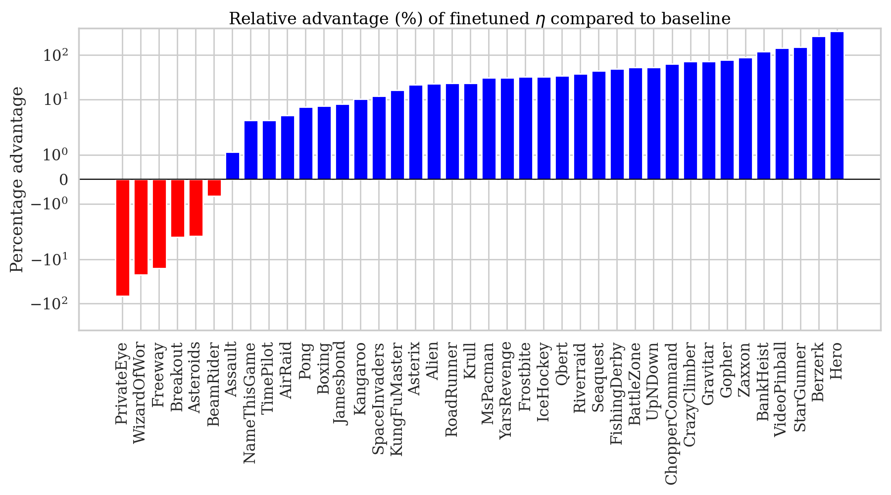
Figure 1: Relative advantage of the finetuned shape scale versus baseline ($\eta=0$) performance. Each environment, for each shape-scale parameter ${\eta\in\{0,0.5,1,2,3,5,10\}}$, is run with five seeds, and the best (in terms of mean score) non-zero $\eta$ value is chosen.

In this section, we derive some theoretical properties of BSRS. Specifically, we show that under appropriate scaling values (“shape-scales”) $\eta$, continual shaping in fact converges despite constant changes in the potential function during training. To prove this result, we employ usual techniques for contraction mappings. For this algorithm, we can directly calculate the asymptotic value functions and potential functions, which can be written in terms of the original un-shaped MDP’s optimal value function. We then show that BSRS is not equivalent to a constant shaping mechanism for any potential function; confirming that BSRS is a novel technique that cannot be replicated by a finetuned choice of potential function. Finally, we provide alternative interpretations of BSRS by re-considering the implied parameter updates under TD(0) and SARSA(0) learning rules.

For completeness, we provide the proof of this result below to give further insight on the mechanism at play and the Theorem’s conclusions.

Proof.

First we prove that the stated operator is indeed a contraction, before calculating the asymptotic potential and value functions. Consider step $n$ of training, where the new value function $Q^{(n)}$ is calculated from the previous iteration $Q^{(n-1)}$ via the Bellman backup equation, using PBRS with potential function $\Phi^{(n-1)}$:

$$Q^{(n)}(s,a) =\left(r(s,a)-\Phi^{(n-1)}(s)\right)+$$

$$\gamma\operatorname*{\mathbb{E}}_{s^{\prime}\sim{}p(\cdot|s,a)}\left(\max_{a^{\prime}}Q^{(n-1)}(s^{\prime},a^{\prime})+\Phi^{(n-1)}(s^{\prime})\right).$$

With the choice of potential specified by BSRS: ${\Phi^{(n-1)}(s)=\eta\max_{a}Q^{(n-1)}(s,a)}$, the corresponding Bellman operator above may be written as:

$$\mathcal{T}Q(s,a) =\left(r(s,a)-\eta\max_{a}Q(s,a)\right)$$

$$+\gamma(1+\eta)\operatorname*{\mathbb{E}}_{s^{\prime}\sim{}p(\cdot|s,a)}\max_{a^{\prime}}Q(s^{\prime},a^{\prime}).$$

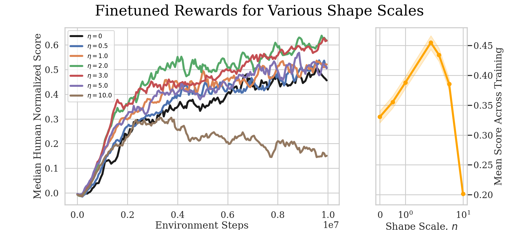
Figure 2: Learning curves for 10M steps in the Atari suite. We take the median human-normalized score over all $40$ environments (shown in Figure 1). In the right panel, a sensitivity plot is given, showing that an intermediate value of $\eta\approx 2$ gives the best performance in aggregate (mean of the median human-normalized score over all environment steps).

To ensure that the Bellman operator with shaping (denoted $\mathcal{T}$ above) is indeed a contraction, we must verify that each application of the shaped Bellman operator reduces the distance between functions in the sup-norm. That is, we require ${|\mathcal{T}U-\mathcal{T}W|_{\infty}\leq\alpha|U-W|_{\infty}}$ to hold for some $\alpha\in[0,1)$, for all bounded functions $U$ and $W$. Proceeding directly with the calculation we find:

$$\big{|}\mathcal{T}U-\mathcal{T}W\big{|}_{\infty}$$

$$=\biggr{|}-\eta\max_{a}U(s,a)+\gamma(1+\eta)\operatorname*{\mathbb{E}}_{s^{\prime}\sim{}p}\max_{a^{\prime}}U(s^{\prime},a^{\prime})$$

$$\quad+\eta\max_{a}W(s,a)-\gamma(1+\eta)\operatorname*{\mathbb{E}}_{s^{\prime}\sim{}p}\max_{a^{\prime}}W(s^{\prime},a^{\prime})\biggr{|}_{\infty}$$

$$=\biggr{|}-\eta\left(\max_{a}U(s,a)-\max_{a}W(s,a)\right)$$

$$\quad+\gamma(1+\eta)\left(\operatorname*{\mathbb{E}}_{s^{\prime}\sim{}p}\max_{a^{\prime}}U(s^{\prime},a^{\prime})-\operatorname*{\mathbb{E}}_{s^{\prime}\sim{}p}\max_{a^{\prime}}W(s^{\prime},a^{\prime})\right)\biggr{|}_{\infty}$$

$$\leq|\eta|\times\biggr{|}\max_{a}U(s,a)-\max_{a}W(s,a)\biggr{|}_{\infty}$$

$$\quad+\gamma|1+\eta|\times\biggr{|}\operatorname*{\mathbb{E}}_{s^{\prime}\sim{}p}\max_{a^{\prime}}U(s^{\prime},a^{\prime})-\operatorname*{\mathbb{E}}_{s^{\prime}\sim{}p}\max_{a^{\prime}}W(s^{\prime},a^{\prime})\biggr{|}_{\infty}$$

$$\leq|\eta|\times\big{|}U-W\big{|}_{\infty}$$

$$\quad+\gamma|1+\eta|\times\mathbb{E}_{s^{\prime}\sim{}p}\biggr{|}\max_{a^{\prime}}U(s^{\prime},a^{\prime})-\max_{a^{\prime}}W(s^{\prime},a^{\prime})\biggr{|}_{\infty}$$

$$\leq(|\eta|+\gamma|1+\eta|)\big{|}U-W\big{|}_{\infty},$$

where the third line follows from the triangle inequality, and remaining lines follow the typical proof for the Bellman operator being a contraction.

Now to enforce the contractive nature of $\mathcal{T}$, we must have the constant factor ${\alpha\doteq|\eta|+\gamma|1+\eta|\in[0,1)}$, which can be solved for $\eta$. The inequality is satisfied for a choice of $\eta$ in the stated range:

$${\eta~\in\biggr{(}-1,\frac{1-\gamma}{1+\gamma}\biggr{)}}.$$ (10)

With the contractive nature of $\mathcal{T}$ verified, we invoke Banach’s fixed point theorem stating that $\mathcal{T}$ has a unique fixed point. Denoting $\mathcal{T}^{\infty}Q(s,a)=Q^{\infty}(s,a)$ as the fixed point and $V^{\infty}(s)=\max_{a}Q^{\infty}(s,a)$ as the associated state value function, we can find the corresponding asymptotic potential function ${\Phi^{\infty}(s)}$ by solving the following self-consistent equation,

$$\Phi^{\infty}(s)=\eta\max_{a}\mathcal{T}Q^{\infty}(s,a)=\eta V^{\infty}(s)$$ (11)

where $Q^{\infty}$ depends implicitly on $\Phi^{\infty}$. More explicitly, we can calculate the right-hand side of this self-consistent equation starting from $Q^{\infty}$ and then taking a maximum over action space:

$$\mathcal{T}Q^{\infty}(s,a) =\left(r(s,a)+\gamma\eta\operatorname*{\mathbb{E}}_{s^{\prime}\sim{}p}V^{\infty}(s^{\prime})-\eta V^{\infty}(s)\right)$$

$$\quad+\gamma\operatorname*{\mathbb{E}}_{s^{\prime}\sim{}p}\max_{a^{\prime}}Q^{\infty}(s^{\prime},a^{\prime})$$

$$=r(s,a)+\gamma(1+\eta)\operatorname*{\mathbb{E}}_{s^{\prime}\sim{}p}V^{\infty}(s^{\prime})-\eta V^{\infty}(s).$$

Taking the max over actions, we have:

$$(1+\eta)V^{\infty}(s) =\max_{a}\left\{r(s,a)+\gamma(1+\eta)\operatorname*{\mathbb{E}}_{s^{\prime}\sim{}p}V^{\infty}(s^{\prime})\right\}.$$

Now we notice that a similar equation is solved by $V_{0}$ when $\eta=0$. Thus, if we assume the form $V_{0}=(1+\eta)V^{\infty}$, then the previous equation is satisfied:

$$(1+\eta)V^{\infty}(s) =\max_{a}\left\{r(s,a)+\gamma\operatorname*{\mathbb{E}}_{s^{\prime}\sim{}p}V_{0}(s^{\prime})\right\}$$

$$(1+\eta)V^{\infty}(s) =V_{0}(s)$$

$$V^{\infty}(s) =\frac{V_{0}(s)}{1+\eta},$$

which is consistent with the aforementioned assumption. Now to solve for the fixed point, $Q^{\infty}$, we write out the backup equation from above, and insert the known expression for $V^{\infty}$:

$$Q^{\infty}(s,a) =r(s,a)+\gamma(1+\eta)\operatorname*{\mathbb{E}}_{s^{\prime}\sim{}p}V^{\infty}(s^{\prime})-\eta V^{\infty}(s)$$

$$=r(s,a)+\gamma\operatorname*{\mathbb{E}}_{s^{\prime}\sim{}p}V_{0}(s^{\prime})-\frac{\eta}{1+\eta}V_{0}(s)$$

$$=Q_{0}(s,a)-\frac{\eta}{1+\eta}V_{0}(s)$$

Calculating the associated asymptotic potential gives, as stated above,

$$\Phi^{\infty}(s) =\eta\max_{a}Q_{\infty}(s,a)=\frac{\eta}{1+\eta}V_{0}(s).$$

∎

We note that due to Theorem 1 of (Adamczyk et al. 2023a), the previous result readily extends to the case of entropy-regularized RL.

Initialization

The previous proofs, in addition to the results of (Wiewiora 2003), suggest that the shaping method used is equivalent to a particular $Q$-table initialization, based on the shaping function:

$$Q^{(0)}(s,a)=\Phi^{\infty}(s)=\frac{V^{*}(s)}{1+\eta}.$$

However, the results in (Wiewiora 2003) were only proven for static potentials which do not change over the course of training. In fact, we find that BSRS is not equivalent to shaping with any static potential, as clarified in the following remark (whose proof is given in the Appendix):

Remark 3.

It can be shown that no equivalent static potential function exists with the same resulting updates as our BSRS potential.

Interpretation as Un-Shaped Learning Problem

The work of (Amit, Meir, and Ciosek 2020) showcased the connection between regularized algorithms and variable discount factors. In this section we take inspiration from their results and proof techniques to provide similar results for our setting.

Proposition 4 (Scaled TD(0) Equivalence).

Let $\theta$ denote the parameters of the value function $V_{\theta}(s)$. The self-shaping algorithm, with shape-scale $\eta$ produces the same set of updates as an un-shaped problem setting, with a rescaled learning rate $\alpha\to\alpha(1+\eta)$ and rescaled reward function $r\to r/(1+\eta)$.

Proof.

The proof follows the same techniques as the proof of Proposition 1 in (Amit, Meir, and Ciosek 2020), without any extra regularization terms. ∎

This proposition suggests (at least for TD(0) value learning) that BSRS is equivalent to solving an appropriately rescaled MDP. Since we are operating in the un-regularized objective setting, a reward function being rescaled by a positive constant (which is enforced by the bounds on $\eta$) leaves the optimal policy invariant.

However, our FA experiments do not employ TD(0) learning. Instead, we perform a SARSA-style update to the $Q$ network. Thus, although the previous proposition can provide some basic intuition, the true learning dynamics with self-shaping is more nuanced. Some of this nuance is captured in the following proposition, which extends the previous result from the TD setting to the SARSA setting.

Proposition 5 (Regularized SARSA(0) Equivalence).

Let $\theta$ denote the parameters of the value function $Q_{\theta}(s,a)$. Suppose the state-value function is calculated from $Q_{\theta}$ with a stop-gradient. The BSRS algorithm with shape-scale $\eta$ produces the same set of updates as an un-shaped problem setting, with a rescaled learning rate $\alpha\to\alpha(1+\eta)$, rescaled reward function $r\to r/(1+\eta)$, and regularized objective, with $\ell_{2}$-regularization on the advantage function.

Function Approximation for $\Phi$

Interestingly, we find that using the online, as opposed to target, network for calculating the potential drastically improves performance. This contradicts the expectation that the “stability” introduced by the target network should be beneficial for calculating a stable potential function. Rather, we find empirically that it is better to use the more rapidly updated online network to calculate $\Phi$. This is also in contradiction to Proposition 5, which assumed the target network is used to calculate the potential. Nevertheless, the proof in the Appendix gives (in the penultimate line) the regularization term $A_{\theta}(s,a)\nabla_{\theta}Q_{\theta}$ when an online network is used for calculating the potential function.

Experiments

In our experiments, we consider the “self-shaped” version of the vanilla value-based algorithm DQN (Mnih et al. 2015; Raffin et al. 2021). We evaluate the performance of our self-shaped algorithm (BSRS) on a variety of environments in a tabular setting, the Atari suite, and on a continuous control task with TD3 (Fujimoto, Hoof, and Meger 2018).

Tabular Setting

In the tabular setting, we can exactly solve the MDP and compare the shaped results to un-shaped learning curves and value functions for verification of the theory. We find that the $Q$-values diverge near the correct boundaries of $\eta$, but our experiments suggest that the allowed range for $\eta$ can potentially be expanded (in the positive direction) beyond the values given above.

We plot the performance (in terms of number of steps until convergence) in Figure 3. The shaded region indicates the standard deviation across 5 random initializations of the $Q$-table. The inset plot shows the $7\times 7$ gridworld with sparse rewards used for this experiment (arrows indicate the optimal policy). Interestingly, we find that for much larger values of $\eta$ ($\approx 3$ times larger than the allowed maximum value) the performance continually improves, with an optimal value achieving roughly $20\%$ reduction in the number of required steps. The relative location of the optimal performance is robust to various environments, stochasticity, and discount factors. This phenomenon seems loosely analogous to the discussion on learning at the “Edge of Stability” in recent literature (Cohen et al. 2021; Ahn et al. 2024), but the exact connection is still unclear.

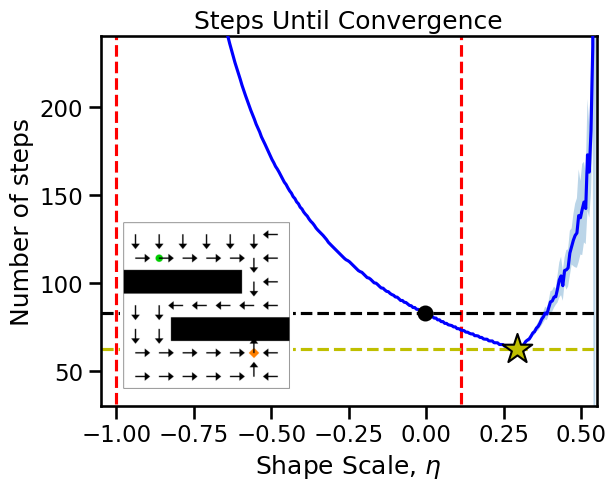
Figure 3: Upon solving the self-shaped Bellman equation in the tabular setting (for environment at inset, $\gamma=0.8$), we find that increasingly large (even beyond the proven range, shown with red dashed lines) values of $\eta$ allows for improved performance. We define “convergence” in this case as the point at which error between iterates in the sup-norm falls below $10^{-6}$. On the $y$-axis, “steps” refers to the number of applications of the self-shaped Bellman operator before convergence. Each point on the curve corresponds to an average over $20$ random initializations.

Continuous Setting

For more complex environments, we use the Arcade Learning Environment suite (Bellemare et al. 2013). The results of these experiments are shown in Figures 1 and 2. Across many environments, BSRS leads to an improvement over the baseline DQN performance ($\eta=0$). In $21/40$ environments we find an improvement of more than $10\%$ and $5/40$ environments show an improvement of over $100\%$. In only $6/40$ environments does self-shaping have a negative impact. If $\eta$ is to be tuned over, one can simply choose $\eta=0$ for these environments. In Figure 2 we find an improvement in the aggregate reward curves of $45\%\to 60\%$ human normalized score. We find that the value of $\eta$ can only be increased up until a point ($\eta\approx 2$) until the performance deteriorates. Although our Theorem 2 suggests that $\eta$ can be negative, we found that the performance in this regime is even worse than that observed for $\eta=10$. Overall, we find a substantial speedup at small times ($\sim{}1.5$M steps) and a lasting improvement in rewards at long times for multiple $\eta$ values.

To test BSRS in the continuous action setting, we use Pendulum-v1 by extending an implementation of TD3 (Raffin et al. 2021). Since TD3 directly maintains an estimate of both the policy and the value function, the latter is used to derive the dynamic shaping potential, $\Phi(s)$. In principle, one must maximize over a continuous set of actions at each timestep to calculate $\Phi$, which becomes intractable, so we instead use the action sampled by the actor. The addition of BSRS to TD3 shows promising improvements over the baseline ($\eta=0$) with a notably more robust performance over a range of large $\eta$ values:  Fig. 4 and inset. We also show the result for $\eta<0$ in the inset, which leads to worse performance in all the FA settings considered. Further experiments are shown in the Appendix.

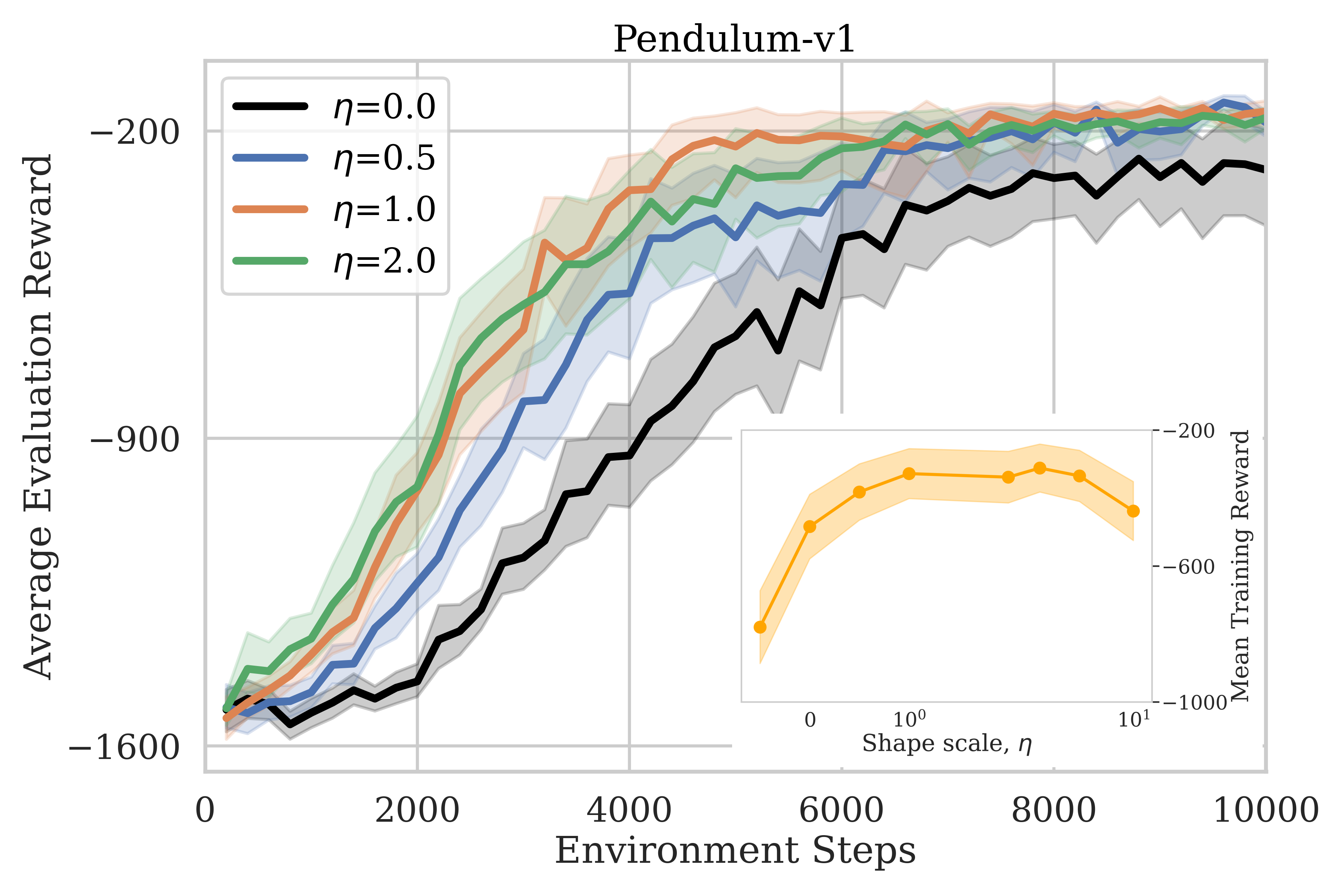
Figure 4: TD3 with BSRS is tested on a continuous control task, Pendulum-v1. Inset: Robustness to varying $\eta$. Results for each $\eta$ value were averaged over $20$ runs (standard error indicated by shaded region).

Discussion

In this work, we provided a theoretically-grounded choice for a dynamic potential function. This work fills the gap in existing literature by providing a universally applicable form for the potential function in any environment. Notably, rather than attempting to tune over the function class $\Phi:\mathcal{S}\to\mathbb{R}$, we instead suggest to tune over the significantly simpler scalar class $\eta\in\mathbb{R}$. This idea simplifies the problem of choosing a potential function from a high-dimensional search problem to a single hyperparameter optimization.

Future work can naturally extend the results presented. For instance, one may study techniques to learn the optimal value of $\eta$ over time, perhaps analogous to the method of learning the $\alpha$ value in (Haarnoja et al. 2018). Further theoretical work can be pursued for understanding the convergence properties of BSRS. For instance, it appears numerically that values of $\eta$ beyond the proven bounds can be used. Also, it is straightforward to see in the proof of Theorem 2 that all instances of $\eta$ may be replaced with the functional $\eta(s)$, giving further control over the self-shaping mechanism. Future work may study such state-dependent shape scales, e.g. dependent on visitation frequencies or the loss experienced in such states (cf. (Wang et al. 2024)), which can further connect to the problem of exploration.

Overall, our work provides a practically relevant implementation of PBRS which provides an advantage in training for both tabular and deep RL.

Appendix A Proofs

Proof of Remark 3

Proof.

We will proceed by contradiction. Suppose there exists a static function $\Psi(s)$ such that all iterations of BSRS are in agreement with the fixed potential $\Psi(s)$. Then, at steps $n-1$ and $n$ of training (two applications of the Bellman operator), the following equations must agree for some choice of $\Psi(s)$:

$$r(s,a)+\gamma\max_{a^{\prime}}\left\{r(s^{\prime},a^{\prime})+\gamma\left(V^{(n-1)}(s^{\prime\prime})+\Psi(s^{\prime\prime})\right)-\Psi(s^{\prime})\right\}+\gamma\Psi(s^{\prime})-\Psi(s)$$ (12)

$$r(s,a)+\gamma\underbrace{\max_{a^{\prime}}\left\{r(s^{\prime},a^{\prime})+\gamma\left((1+\eta)V^{(n-1)}(s^{\prime\prime})\right)-\eta V^{(n-1)}(s^{\prime})\right\}}_{V^{(n)}(s^{\prime})}+\gamma\eta V^{(n)}(s^{\prime})-\eta V^{(n)}(s)$$ (13)

This is equivalent to the following equations agreeing (simplifying shared terms and canceling subsequent potentials in the static case):

$$\gamma\max_{a^{\prime}}\left\{r(s^{\prime},a^{\prime})+\gamma\left(V^{(n-1)}(s^{\prime\prime})+\Psi(s^{\prime\prime})\right)\right\}-\Psi(s)$$ (14)

$$\gamma\max_{a^{\prime}}\left\{r(s^{\prime},a^{\prime})+\gamma\left((1+\eta)V^{(n-1)}(s^{\prime\prime})\right)-\eta V^{(n-1)}(s^{\prime})\right\}+\gamma\eta V^{(n)}(s^{\prime})-\eta V^{(n)}(s)$$ (15)

Since the reward function is arbitrary and the equation must hold for all states, the inner terms must agree:

$$V^{(n-1)}(s^{\prime\prime})+\Psi(s^{\prime\prime})=(1+\eta)V^{(n-1)}(s^{\prime\prime}),$$ (16)

and so we must have the relation

$$\Psi(s)=\eta V^{(n-1)}(s),$$ (17)

which is inconsistent as a static potential function, and also is in disagreement with the relation implied by the outer terms:

$$\Psi(s)=-\gamma\eta V^{(n-1)}(s^{\prime})+\gamma\eta V^{(n)}(s^{\prime})-\eta V^{(n)}(s).$$ (18)

Explicitly, we now see the disconnect is caused by the difference between subsequent value functions:

$$\gamma\eta\left(V^{(n)}(s^{\prime})-V^{(n-1)}(s^{\prime})\right)\neq 0,$$ (19)

which controls the error in the constant-potential function. ∎

Proof of Proposition 5

Proof.

We write out the difference between successive parameters, using the same proof technique as in (Amit, Meir, and Ciosek 2020):

$$\theta^{\prime}-\theta =\alpha\nabla_{\theta}Q_{\theta}(s,a)\left[r+\gamma\Phi(s^{\prime})-\Phi(s)+\gamma V(s^{\prime})-Q_{\theta}(s,a)\right]$$

$$=\alpha\nabla_{\theta}Q_{\theta}(s,a)\left[r+\gamma\eta V(s^{\prime})-\eta V(s)+\gamma V(s^{\prime})-Q_{\theta}(s,a)\right]$$

$$=\alpha(1+\eta)\nabla_{\theta}Q_{\theta}(s,a)\left[\frac{r}{1+\eta}+\gamma V(s^{\prime})-\frac{\eta}{1+\eta}V(s)-\frac{Q_{\theta}(s,a)}{1+\eta}\right]$$

$$=\widetilde{\alpha}\biggr{(}\nabla_{\theta}Q_{\theta}(s,a)\left[\widetilde{r}+\gamma V(s^{\prime})-Q_{\theta}(s,a)\right]+\nabla_{\theta}Q_{\theta}(s,a)\left[-\frac{\eta}{1+\eta}V(s)+\frac{\eta}{1+\eta}Q_{\theta}(s,a)\right]\biggr{)}$$

$$=\widetilde{\alpha}\biggr{(}\nabla_{\theta}Q_{\theta}(s,a)\left[\widetilde{r}+\gamma V(s^{\prime})-Q_{\theta}(s,a)\right]+\frac{\eta}{1+\eta}A_{\theta}(s,a)\nabla_{\theta}Q_{\theta}(s,a)\biggr{)}$$

$$=\widetilde{\alpha}\biggr{(}\nabla_{\theta}Q_{\theta}(s,a)\left[\widetilde{r}+\gamma V(s^{\prime})-Q_{\theta}(s,a)\right]+\lambda\nabla_{\theta}A^{2}_{\theta}(s,a)\biggr{)}$$

We denote the regularization coefficient as $\lambda\doteq\frac{1}{2}\frac{\eta}{1+\eta}$. The last line follows if we assume that the gradient has no effect on the state value function (i.e. $V(s)$ is calculated via the target network or a stop-gradient operation is used):

$$\nabla_{\theta}A_{\theta}(s,a)=\nabla_{\theta}\left(Q_{\theta}(s,a)-V(s)\right)=\nabla_{\theta}Q_{\theta}(s,a).$$ (20)

∎

Appendix B Experiment Details

We extend DQN and TD3 from Stable-baselines3 (Raffin et al. 2021) to include BSRS, by changing the definition of reward values before the target values are calculated.

Hyperparameters

For the Atari environments, we use all the hyperparameters from (Mnih et al. 2015). Each run is trained for $10$M steps. All runs are averaged over $5$ random initializations in every environment. This yields a compute cost of roughly $10^{7}$ steps/run $\times 5$ runs/env. $\times 40$ envs. $\times 7$ shape-scales $\times 1/100$ sec./step $\approx 1600$ GPU-days. Training was performed across clusters with various resources, including A100s, V100s, and RTX 30 & 40 series GPUs. We use the standard set of Atari wrappers. Specifically, this include no-op reset, frame skipping (4 frames), max-pooling of two most recent observations, termination signal when a life is lost, resize to $84\times 84$, grayscale observation, clipped reward to $\{-1,0,1\}$, frame stacking (4 frames) and image transposing.

Parameter	Value
Batch Size	$32$
Buffer Size	$100,000$
Discount Factor ($\gamma$)	$0.99$
Gradient Steps	$1$
Learning Rate	$0.0001$
Target Update Interval	$1,000$
Train Frequency	$4$
Learning Starts	$50,000$
Exploration Fraction	$0.1$
Exploration Initial $\epsilon$	$1.0$
Exploration Final $\epsilon$	$0.02$
Discount Factor ($\gamma$)	$0.99$
Total Timesteps	$10,000,000$

Table 1: Shared hyperparameter settings used in our ALE experiments for all values of $\eta\in\{0.0,0.5,1.0,2.0,3.0,5.0,10.0\}$.

For the Pendulum environment, we use TD3’s default hyperparameters with a few modifications, based on hyperparameters published by (Raffin et al. 2021):

Parameter	Value
Batch Size	$256$
Buffer Size	$200,000$
Discount Factor ($\gamma$)	$0.98$
Gradient Steps	$-1$
Learning Rate	$0.001$
Learning Starts	$0$
Train Frequency	$1$
Policy Delay	$2$
Target Policy Noise	$0.2$
Target Noise Clip	$0.5$

Table 2: TD3 hyperparameters for Pendulum-v1 for all values of $\eta\in\{-0.5,0.0,0.5,1.0,2.0,3.0,5.0,10.0\}$.

Each run is trained for $20$k steps. All runs are averaged over $20$ random initializations in every environment. This yields a compute cost of roughly $10^{4}$ steps/run $\times 20$ runs/env. $\times 8$ shape-scales $\times 1/100$ sec./step $\approx 6$ GPU-hours. Training was performed locally with a single RTX 3080.

Appendix C Additional Experiments

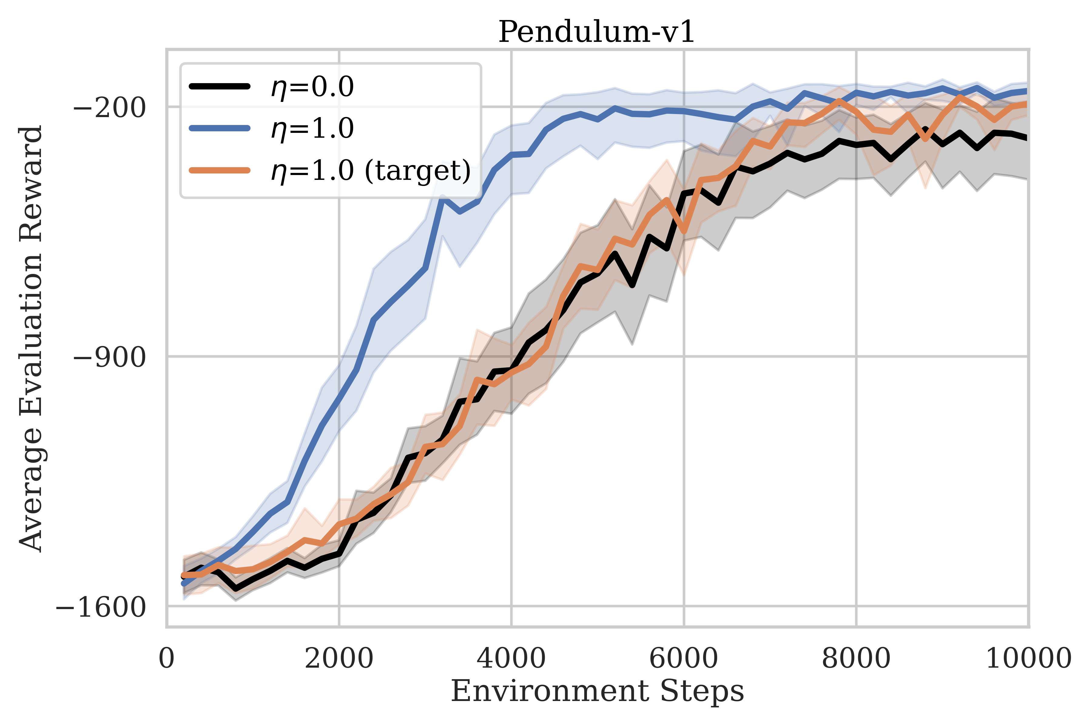
Figure 5: We also test using the target network to calculate $\Phi(s)$, rather than the online critic network. We find that despite the initial intuition that a target network may help stabilize the otherwise fast-changing reward structure, the use of the online network to derive $\Phi(s)$ is crucial to see a (positive) performance difference, at least in the settings considered here.

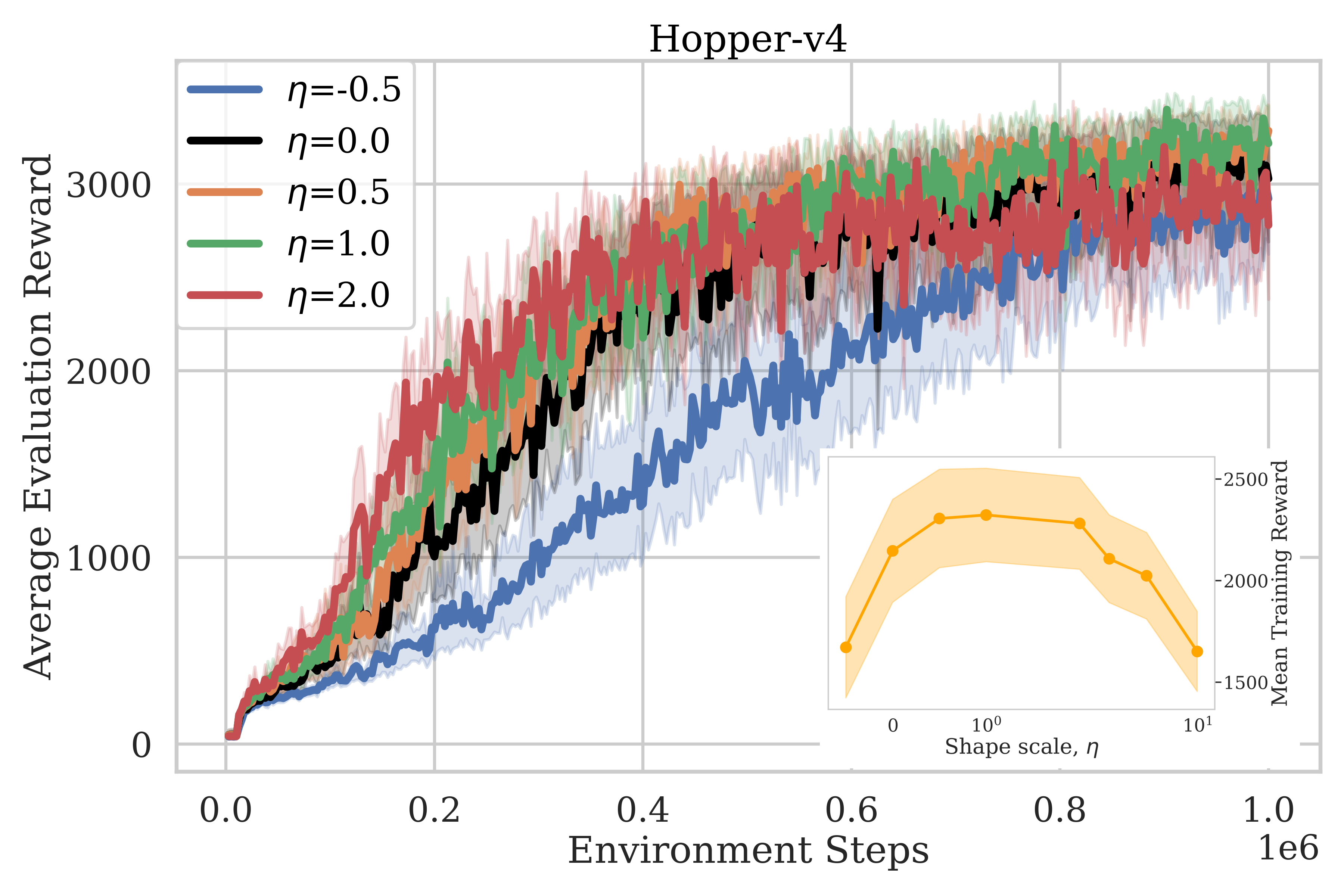
(a) TD3 with BSRS on Hopper-v4.

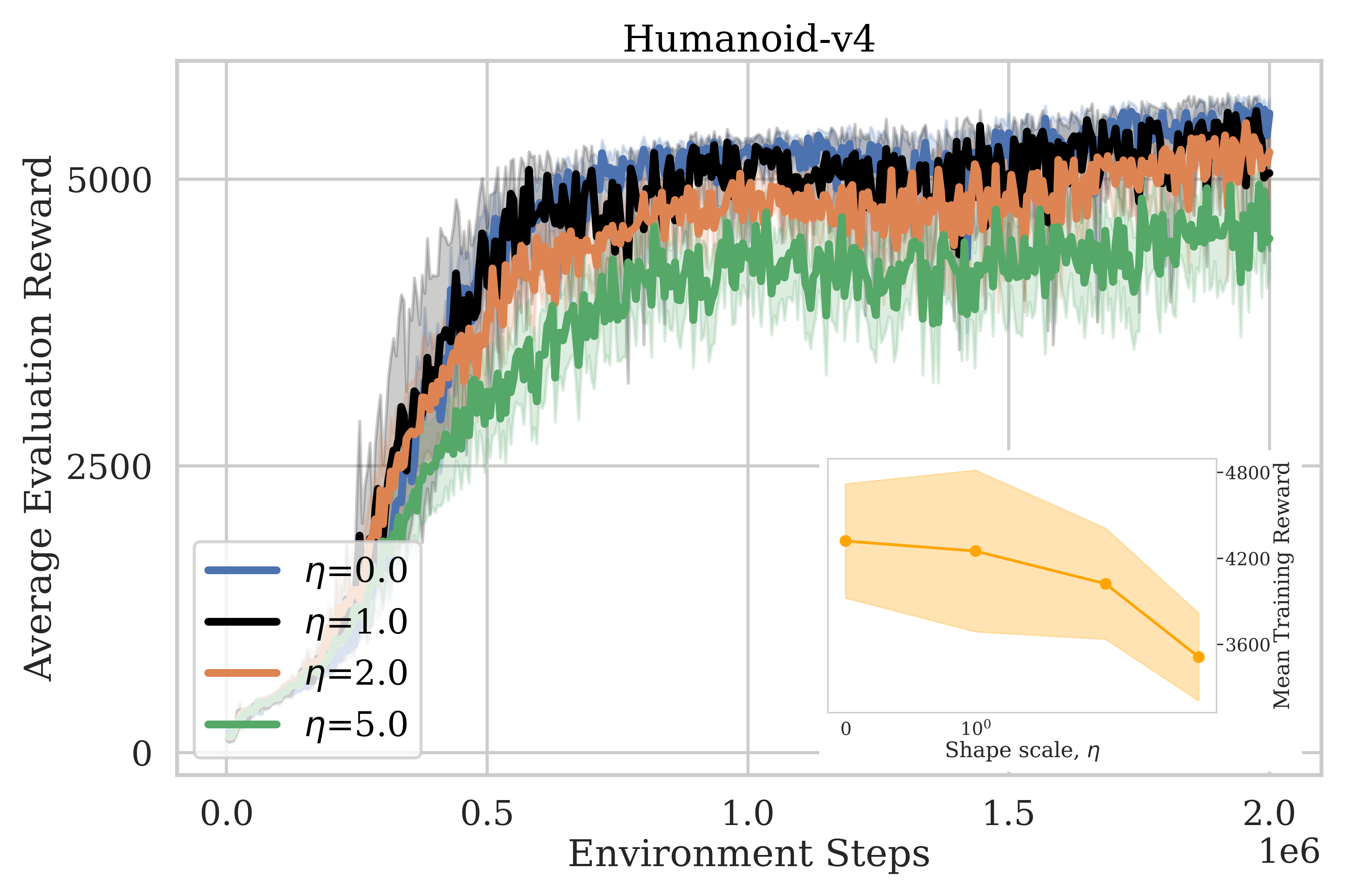
(b) TD3 with BSRS on Humanoid-v4.

Figure 6: We also test BSRS on TD3 for more complex continuous action tasks. The performance is slightly better (at least for Hopper-v4) for an optimized value of $\eta$, but potentially within the margin of statistical significance. The hyperparameters are the same as those of Pendulum (shown in Table 2) except for the learning rate of $3\times 10^{-4}$ and an updated “learning starts” value of $10,000$ steps. For Humanoid-v4, we did not find a statistically significant improvement for the values of $\eta$ tested; however, we believe this may be improved in future work. As discussed in the main text, ideas for further improvement include: further hyperparameter tuning, state-dependent scale parameter $\eta(s)$, and dynamic schedules for the scaling parameter. Training was distributed locally and on clusters (with RTX 20, 30, and 40 series), totaling roughly 400 GPU-hours of compute.

References

- Adamczyk et al. (2023a) Adamczyk, J.; Arriojas, A.; Tiomkin, S.; and Kulkarni, R. V. 2023a. Utilizing Prior Solutions for Reward Shaping and Composition in Entropy-Regularized Reinforcement Learning. Proceedings of the AAAI Conference on Artificial Intelligence, 37(6): 6658–6665.
- Adamczyk et al. (2023b) Adamczyk, J.; Makarenko, V.; Arriojas, A.; Tiomkin, S.; and Kulkarni, R. V. 2023b. Bounding the optimal value function in compositional reinforcement learning. In Evans, R. J.; and Shpitser, I., eds., Proceedings of the Thirty-Ninth Conference on Uncertainty in Artificial Intelligence, volume 216 of Proceedings of Machine Learning Research, 22–32. PMLR.
- Adamczyk et al. (2024) Adamczyk, J.; Makarenko, V.; Tiomkin, S.; and Kulkarni, R. V. 2024. Boosting Soft Q-Learning by Bounding. Reinforcement Learning Journal, 5: 2373–2399.
- Ahn et al. (2024) Ahn, K.; Bubeck, S.; Chewi, S.; Lee, Y. T.; Suarez, F.; and Zhang, Y. 2024. Learning threshold neurons via edge of stability. Advances in Neural Information Processing Systems, 36.
- Amit, Meir, and Ciosek (2020) Amit, R.; Meir, R.; and Ciosek, K. 2020. Discount factor as a regularizer in reinforcement learning. In International conference on machine learning, 269–278. PMLR.
- Bellemare et al. (2013) Bellemare, M. G.; Naddaf, Y.; Veness, J.; and Bowling, M. 2013. The arcade learning environment: An evaluation platform for general agents. Journal of Artificial Intelligence Research, 47: 253–279.
- Cao, Cohen, and Szpruch (2021) Cao, H.; Cohen, S.; and Szpruch, Ł. 2021. Identifiability in inverse reinforcement learning. Advances in Neural Information Processing Systems, 34: 12362–12373.
- Centa and Preux (2023) Centa, M.; and Preux, P. 2023. Soft action priors: towards robust policy transfer. Proceedings of the AAAI Conference on Artificial Intelligence, 37(6): 6953–6961.
- Cohen et al. (2021) Cohen, J.; Kaur, S.; Li, Y.; Kolter, J. Z.; and Talwalkar, A. 2021. Gradient descent on neural networks typically occurs at the edge of stability. In International Conference on Learning Representations.
- Cooke et al. (2023) Cooke, L. H.; Klyne, H.; Zhang, E.; Laidlaw, C.; Tambe, M.; and Doshi-Velez, F. 2023. Toward computationally efficient inverse reinforcement learning via reward shaping. arXiv preprint arXiv:2312.09983.
- Devlin and Kudenko (2012) Devlin, S. M.; and Kudenko, D. 2012. Dynamic potential-based reward shaping. In 11th International Conference on Autonomous Agents and Multiagent Systems (AAMAS 2012), 433–440. IFAAMAS.
- Fujimoto, Hoof, and Meger (2018) Fujimoto, S.; Hoof, H.; and Meger, D. 2018. Addressing function approximation error in actor-critic methods. In International conference on machine learning, 1587–1596. PMLR.
- Gao and Toni (2015) Gao, Y.; and Toni, F. 2015. Potential based reward shaping for hierarchical reinforcement learning. In Twenty-Fourth International Joint Conference on Artificial Intelligence.
- Gleave et al. (2021) Gleave, A.; Dennis, M.; Legg, S.; Russell, S.; and Leike, J. 2021. Quantifying differences in reward functions. International Conference on Learning Representations.
- Grześ and Kudenko (2010) Grześ, M.; and Kudenko, D. 2010. Online learning of shaping rewards in reinforcement learning. Neural networks, 23(4): 541–550.
- Gupta et al. (2022) Gupta, A.; Pacchiano, A.; Zhai, Y.; Kakade, S.; and Levine, S. 2022. Unpacking reward shaping: Understanding the benefits of reward engineering on sample complexity. Advances in Neural Information Processing Systems, 35: 15281–15295.
- Haarnoja et al. (2018) Haarnoja, T.; Zhou, A.; Hartikainen, K.; Tucker, G.; Ha, S.; Tan, J.; Kumar, V.; Zhu, H.; Gupta, A.; Abbeel, P.; et al. 2018. Soft actor-critic algorithms and applications. arXiv preprint arXiv:1812.05905.
- Hu et al. (2020) Hu, Y.; Wang, W.; Jia, H.; Wang, Y.; Chen, Y.; Hao, J.; Wu, F.; and Fan, C. 2020. Learning to utilize shaping rewards: A new approach of reward shaping. Advances in Neural Information Processing Systems, 33: 15931–15941.
- Jenner, Skalse, and Gleave (2022) Jenner, E.; Skalse, J. M. V.; and Gleave, A. 2022. A general framework for reward function distances. In NeurIPS ML Safety Workshop.
- Jenner, van Hoof, and Gleave (2022) Jenner, E.; van Hoof, H.; and Gleave, A. 2022. Calculus on MDPs: Potential Shaping as a Gradient. arXiv preprint arXiv:2208.09570.
- Jiang et al. (2021) Jiang, Y.; Bharadwaj, S.; Wu, B.; Shah, R.; Topcu, U.; and Stone, P. 2021. Temporal-logic-based reward shaping for continuing reinforcement learning tasks. In Proceedings of the AAAI Conference on artificial Intelligence, volume 35, 7995–8003.
- Ma et al. (2024) Ma, H.; Luo, Z.; Vo, T. V.; Sima, K.; and Leong, T.-Y. 2024. Highly efficient self-adaptive reward shaping for reinforcement learning. arXiv preprint arXiv:2408.03029.
- Mataric (1994) Mataric, M. J. 1994. Reward Functions for Accelerated Learning. In Cohen, W. W.; and Hirsh, H., eds., Machine Learning Proceedings 1994, 181–189. San Francisco (CA): Morgan Kaufmann. ISBN 978-1-55860-335-6.
- Mnih et al. (2015) Mnih, V.; Kavukcuoglu, K.; Silver, D.; Rusu, A. A.; Veness, J.; Bellemare, M. G.; Graves, A.; Riedmiller, M.; Fidjeland, A. K.; Ostrovski, G.; et al. 2015. Human-level control through deep reinforcement learning. nature, 518(7540): 529–533.
- Naik et al. (2024) Naik, A.; Wan, Y.; Tomar, M.; and Sutton, R. S. 2024. Reward Centering. Reinforcement Learning Journal, 4: 1995–2016.
- Ng, Harada, and Russell (1999) Ng, A. Y.; Harada, D.; and Russell, S. 1999. Policy invariance under reward transformations: Theory and application to reward shaping. In Proceedings of the 16th International Conference on Machine Learning, volume 99, 278–287.
- Raffin et al. (2021) Raffin, A.; Hill, A.; Gleave, A.; Kanervisto, A.; Ernestus, M.; and Dormann, N. 2021. Stable-Baselines3: Reliable Reinforcement Learning Implementations. Journal of Machine Learning Research, 22(268): 1–8.
- Randløv and Alstrøm (1998) Randløv, J.; and Alstrøm, P. 1998. Learning to Drive a Bicycle Using Reinforcement Learning and Shaping. In Shavlik, J. W., ed., Proceedings of the Fifteenth International Conference on Machine Learning (ICML 1998), Madison, Wisconsin, USA, July 24-27, 1998, 463–471. Morgan Kaufmann.
- Skalse et al. (2022) Skalse, J.; Howe, N.; Krasheninnikov, D.; and Krueger, D. 2022. Defining and characterizing reward gaming. Advances in Neural Information Processing Systems, 35: 9460–9471.
- Wang et al. (2024) Wang, Y.; Yang, M.; Dong, R.; Sun, B.; Liu, F.; et al. 2024. Efficient potential-based exploration in reinforcement learning using inverse dynamic bisimulation metric. Advances in Neural Information Processing Systems, 36.
- Wiewiora (2003) Wiewiora, E. 2003. Potential-based shaping and Q-value initialization are equivalent. Journal of Artificial Intelligence Research, 19: 205–208.
- Wulfe et al. (2022) Wulfe, B.; Balakrishna, A.; Ellis, L.; Mercat, J.; McAllister, R.; and Gaidon, A. 2022. Dynamics-aware comparison of learned reward functions. International Conference on Learning Representations.
- Zhang et al. (2021) Zhang, B.; Rajan, R.; Pineda, L.; Lambert, N.; Biedenkapp, A.; Chua, K.; Hutter, F.; and Calandra, R. 2021. On the importance of hyperparameter optimization for model-based reinforcement learning. In International Conference on Artificial Intelligence and Statistics, 4015–4023. PMLR.
- Zou et al. (2021) Zou, H.; Ren, T.; Yan, D.; Su, H.; and Zhu, J. 2021. Learning task-distribution reward shaping with meta-learning. In Proceedings of the AAAI Conference on Artificial Intelligence, volume 35, 11210–11218.