Optimizing Noise Schedules of Generative Models
in High Dimensions
Santiago Aranguri Giulio Biroli Marc Mézard Eric Vanden-Eijnden Courant Institute of Mathematical Sciences, New York University Laboratoire de Physique de l’Ecole Normale Supérieure ENS, Université PSL Department of Computing Sciences, Bocconi University Courant Institute of Mathematical Sciences, New York University
Abstract
Recent works have shown that diffusion models can undergo phase transitions, the resolution of which is needed for accurately generating samples. This has motivated the use of different noise schedules, the two most common choices being referred to as variance preserving (VP) and variance exploding (VE). Here we revisit these schedules within the framework of stochastic interpolants. Using the Gaussian Mixture (GM) and Curie-Weiss (CW) data distributions as test case models, we first investigate the effect of the variance of the initial noise distribution and show that VP recovers the low-level feature (the distribution of each mode) but misses the high-level feature (the asymmetry between modes), whereas VE performs oppositely. We also show that this dichotomy, which happens when denoising by a constant amount in each step, can be avoided by using noise schedules specific to VP and VE that allow for the recovery of both high- and low-level features. Finally we show that these schedules yield generative models for the GM and CW model whose probability flow ODE can be discretized using steps in dimension instead of the steps required by constant denoising.
1 Introduction
Generative models based on dynamical transport of measure have emerged as powerful tools in unsupervised learning ([Sohl-Dickstein et al., 2015], [Ho et al., 2020], [Song et al., 2021]). These models are trained on samples from a data distribution and tasked with generating new samples from this distribution. This can for example be achieved with probability flow ODEs, in which the data samples are used to learn a velocity field that pushes samples from a simple distribution (say a Gaussian) onto new samples from the data distribution. Probability flow ODEs can achieve state of the art performance in image generation [Esser et al., 2024], but they are not fully understood theoretically. A theoretical framework not only would suggest improvements, but also greatly reduce the architecture and hyperparameter search that practitioners must do to get accurate results.
The main sources of error for probability flow ODE are (a) estimating the velocity field for the generative model and (b) running a discretization of this velocity field. In this work, we assume access to the exact velocity field and analyze the error from running the generative model with a discretized version of the velocity field, as the dimension of the input data goes to infinity.
To this end, we build upon the work of [Biroli et al., 2024], where score-based diffusion models are studied and shown to exhibit a phase transition in the generative process. This transition occurs at a time that goes to infinity as the dimension of the data grows, thereby requiring to run the diffusion model for longer times as the dimension increases to capture the transition. Here we revisit these results within the framework of Stochastic Interpolants [Albergo and Vanden-Eijnden, 2023, Albergo et al., 2023] (also see [Lipman et al., 2023] and [Liu et al., 2022]), where the generative process happens in instead of which is the case in [Biroli et al., 2024], and is performed via solving a probability flow ODE. With a uniform noise schedule, we show the solutions to this ODE display a speciation transition a time that goes to zero as the dimension tends to infinity and therefore cannot be resolved by uniform time-discretization of the ODE. However, we also show that we can select an appropriate noise schedule to ensure that this speciation transition is resolved.
Specifically, we analyze the probability flow ODE generating samples from a two-mode Gaussian mixture.
-
•
We shed light into the Variance Preserving (VP) and Variance Exploding (VE) regimes used by practitioners by showing that with a uniform noise schedule, VP captures only the high-level feature whereas VE captures only the low-level feature. We show that with the appropriate noise schedules, VP and VE can capture both phases.
-
•
We find that the velocity field simplifies for each phase, reducing to the estimation of the high-level feature in the beginning and then sharply changing to the estimation of the low-level feature.
-
•
We show that the length of the two phases depends on the initial variance and the time-schedule of the interpolation, which need to be chosen correctly for accurate estimation of both phases. Not doing so leads to either of the phases having length that vanishes as implying that the generative process does not capture some of the features from the data.
-
•
In fact, with the correct initial variance and time schedule, the generative process has a well-defined limiting ODE as . In particular, this means that we get accurate estimation of the data discretizing the generative process using points111We recall that if . If we discretize with a uniform grid, we require points for accurate estimation.
2 Related work
[Biroli and Mézard, 2023] consider the Curie-Weiss model as the data distribution, and introduced the idea of an speciation time, being the time after which the generative process has found the high-level structure of the data. They further find the dependence of the speciation time on the dimension of the data. Later [Biroli et al., 2024] generalize the definition of speciation time, which can be described in terms of cloning trajectories [Biroli et al., 2024] which consists of noising by a certain amount and defining the speciation transition as the amount of noise that is needed to make trajectories with independent Brownian motion terms started at the noisy datapoint speciate (i.e. go to different classes.) See also the related U-Turn method from [Behjoo and Chertkov, 2024] and [Sclocchi et al., 2024]. The present paper builds on their work, and focuses on understanding how the speciation time is affected by time-dilations and the initial variance of the generative process. The correct choice of these leads to a well-defined limiting probability flow ODE as which allows us to characterize the generative model in the different phases.
[Raya and Ambrogioni, 2023] show the existence of spontaneous symmetry breaking, dividing the generative dynamics into two phases: 1) a linear steady-state dynamics around a central fixed-point, 2) an attractor dynamics towards the data manifold. They provide a theoretical analysis supporting their claim for the empirical distribution on undistinguishable samples and for the hypersphere. In the present paper, however, through considering asymptotics and time-dilations, we are able to analyze more complex data distributions, and give exact expressions for the velocity field of the generative model. This allows us to show how each feature of the data is learned, and show that the velocity field simplifies in each phase.
[Li and Chen, 2024] study diffusion models through critical windows, showing that for strongly log-concave data, one can associate a narrow time window to the learning of a given feature of the data. Further, they interpret diffusion models as hierarchical samplers that progressively decide output features. The main differences with our work is that they run the generative model in continuous time, whereas our analysis answers the important practical question of how many discretization steps are needed to capture different features. Our analysis allows us to give precise characterizations of the dynamics in each phase. We can also handle non-log-concave distributions, and we do so for the Curie-Weiss distribution, showing that the separation of phases extends beyond log-concave distributions. As opposed to ours, their analysis is non-asymptotic.
Several works focus on providing bounds for the number of required steps for generative models to accurately generate data. They either have general mild assumptions on the smoothness of the data ([Chen et al., 2023], [Benton et al., 2024]) or closer to our work, assume Gaussian Mixture data ([Gatmiry et al., 2024], [Shah et al., 2023]). They require a polynomial in dimension number of steps for accurate estimation, with the best bound being for the probability flow ODE requiring steps. In the present work we assume a simpler distribution (a two-mode Gaussian Mixture) but we are able to show that if one uses the right noise schedule, steps suffice for accurate estimation of this distribution.
3 Results
3.1 Set up
We consider the Gaussian Mixture (GM) distribution
where such that and
We will benchmark different settings for the probability flow ODE generating samples from the GM distribution testing whether it captures the high-level parameter and low-level parameter More precisely, we consider the stochastic interpolant [Albergo et al., 2023]
where , and The choices of imply that and , that is, interpolates between noise and data. We assume that do not depend on , and will use to scale the noise with dimension. Borrowing terminology from [Song et al., 2021], we will call the stochastic interpolants with the Variance Preserving (VP) interpolants and the Variance Exploding (VE) interpolants.
Associated with any interpolant there is a generative model that pushes through an ODE or an SDE to generate samples from the data distribution. In this setup, [Albergo et al., 2023] prove the following result.
Lemma 1.
Let solve the probability flow ODE
| (1) |
If , then for all , and in particular, .
In practice, the ODE from (1) needs to be discretized. We are interested in how well this probability flow ODE generates samples from the data, when the number of discretization points does not grow with In the next proposition, we consider a VP interpolant, and show that if we discretize with a uniform grid whose step size is we will not recover the parameter However, the VP interpolants are able to recover the distribution within each mode (given by the parameter ).
Proposition 1 (VP only captures ).
Let be obtained from the probability flow ODE (1) associated with a VP interpolant discretized with a uniform grid with step size Let
Then
where
Morevover, for , we have
where satisfies
This proposition can be better understood by looking at the speciation time which is the time in the generative process after which it is determined what mode the sample will belong to. [Biroli et al., 2024] determine the speciation time for the GM distribution, working with score-based diffusion models on We show in appendix, Proposition 3, that translating their result to the context of stochastic interpolants gives that the VP interpolants have speciation time that goes to as goes to infinity, meaning that the time when the generative model can recover the parameter vanishes as the dimension goes to infinity. This explains why the discretization with a finite cannot recover the correct speciation transition.
On the contrary, we prove next that the VE interpolants have speciation time as , and therefore their generative model can recover the correct value of in the limit of going to infinity when discretized with a uniform grid with steps. However, as this generative model with VE interpolants focuses on the speciation transition, it fails to reconstruct the right probability distribution of each mode: it cannot obtain the right value of in the limit.
Proposition 2 (VE only captures ).
Let be obtained from the probability flow ODE (1) associated with the VE interpolant discretized with a uniform grid with step size Let
Then fulfills the ODE
where is such that . This yields a speciation time independent of , and implies that
Moreover, for , we have
where satisfies
Dichotomy between VP and VE interpolants. The discussion so far shows a dichotomy: the is captured by the VE but not the VP interpolant, whereas the is captured by the VP but not the VE interpolant. Next we show how to introduce time dilations to solve this issue.
3.2 Time dilated interpolants
For concretness, we specialize to and We define the Dilated Variance Preserving interpolant
| (2) |
and the Dilated Variance Exploding interpolant
| (3) |
If we think of running a discretization of the probability flow ODE associated to any of these interpolants, we can see each step in the discretization as denoising by a certain amount. Introducing a time dilation, then, is equivalent to using a non-uniform noise schedule. Next, we give specific time dilations for the VP and VE interpolants, which will enable us to capture both and
Dilated Variance Preserving. We saw earlier that the VP interpolants have a speciation times that go to as goes to infinity. In fact, if we prove in the appendix, Proposition 3, that the VP interpolant has speciation time This motivates a time dilation that makes the speciation time happen at a constant time as To this end, we consider
| (4) |
which satisfies where is a constant.
We now prove that with this time dilation, the generative model associated to the VP interpolant has a well-defined limiting ODE. This implies that the dilated VP captures both and
Theorem 1 (Dilated VP captures and ).
Let be obtained from the probability flow ODE associated with the dilated VP interpolant discretized with a uniform grid with step size Then
where is characterized as follows:
First phase: For we have
In addition
fulfills
where is such that This implies
Second phase: For we have
In addition
fulfills, for , the ODE
and satisfies
where is such that
Since we take first and then this means we can discretize the ODE with and get accurate estimation.
We emphasize that the first phase captures the relative asymmetry whereas the second phase captures the distribution of each mode, through the estimation of This result can be equivalently seen as the fact that using a discretization grid for the non-dilated VP interpolant with half grid points on and half on yields accurate estimation of and In particular, this means that using a uniform discretization with grid points gives correct estimation of and for the non-dilated VP interpolant. However, we show in the appendix, Proposition 4, that discretizing the probability flow ODE for the VP interpolant with uniform grid points does not yield correct estimation of
Dilated Variance Exploding. We saw in Proposition 2 that the vanilla VE interpolant can not recover . This can be seen intuitively by looking at the interpolant at a given coordinate
and noting that only for the noise and data have coefficients of the same magnitude. Without dilation, this window disappears as goes to infinity. We prove that dilating time so as to have this window of constant length solves the problem. More precisely, consider the time-dilation
| (5) |
Theorem 2 (Dilated VE captures and ).
Let be obtained from the probability flow ODE associated with the dilated VE interpolant discretized with a uniform grid with step size Let
and let
First phase: For we have
where
Moreover, fulfills
with and is such that This implies
Second phase: For we have that remains constant. Moreover,
where
In particular,
Similarly to Theorem 1, we see that the first phase captures whereas the second phase captures However, we see that the role of the dilation is different in the VP and the VE interpolants. For the VP interpolant, the estimation of is solved “by default,” whereas estimating requires large enough. The VE interpolant performs oppositely.
3.3 Connection with Score-based diffusion models
Variance Preserving SDE. Consider the VP SDE from [Song et al., 2021]
| (6) |
Under this SDE, converges to a standard normal as tends to By learning the score of the density of we can write the associated backward SDE to (6) or the probability flow ODE and use either as a generative model. A computation yields that the law of conditioned on is given by
| (7) |
for This means that is equal in law to
where and Under the change of variables we have
| (8) |
which is a Variance Preserving interpolant with In practice, the following more general SDE is considered
| (9) |
with In this case, under the change of variables we get that equals in law to
where Hence, acts as a time dilation of the first VP interpolant (8).
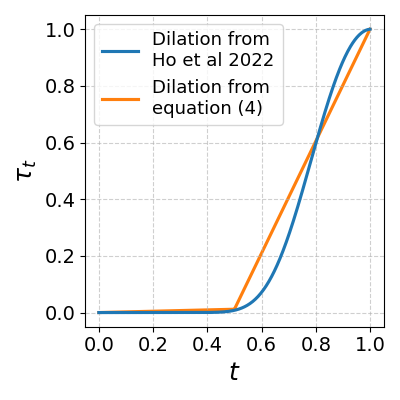
Practitioners often run the SDE (9) for and take where and are determined empirically. We plot in Figure 1 this time dilation using and as chosen by [Ho et al., 2020] and [Song et al., 2021].
Although our analysis for the time dilated VP interpolant is for and we show in the appendix, Theorem 5, that the VP interpolant with and also captures both and when using the time dilation from equation (4).
We see in Figure 1 that the dilation from [Ho et al., 2020] and our dilation from equation (4) both dilate near the beginning. This suggests that our analysis may extend to broader settings beyond the probability flow ODE for the Gaussian Mixture distribution.

Variance Exploding SDE. The VE SDE is defined as
where for It can be seen that conditioned on is given by
Hence, defining we get
| (10) |
where and Taking gives In practice, is taken to be a small constant, usually while is taken to be the maximum Euclidean distance between any pair of sample from the dataset [Song and Ermon, 2020]. For the GM distribution, this distance is of order This means that the VE SDE from [Song et al., 2021] and our VE interpolant both start from a noise distribution with variance
In Figure 1 we plot the magntiude of the noise in the interpolation. For our dilated VE interpolant, this is where is given in (5). For the coming from the VE SDE, we get from (10) that We note that our time dilation makes for and a similar behavior is achieved using the noise magnitude from the VE SDE.
3.4 Curie-Weiss distribution
We let and let
where are Ising spins and is inverse temperature chosen such that We define the Curie-Weiss (CW) distribution as
For its magnetization is defined as We note that in the limit, this magnetization is the same (up to a factor of ) as the magnetization with Hence if we pick both the GM and CW distributions are alike in that they consist of two modes with probability and However, they differ in the details: in particular, one is -valued while the other is -valued.
The same proof technique from Proposition 1 and 2 can be used to show that for the CW distribution without time dilating, the VP interpolant can not capture the parameter and the VE interpolant can not capture the distribution of the spins. However, we show next that we can solve this problem by using the same dilation for the VE interpolant from equation (5) that we used to capture and for the GM distribution. (See the appendix, Theorem 4, for an analogous claim for the dilated VP interpolant.)
Theorem 3 (Dilated VE captures both features for CW).
Let be obtained from the probability flow ODE associated with the dilated VE interpolant for the CW distribution discretized with a uniform grid with step size Let and
and let
First phase: For we have that fulfills
with and is such that In particular,
In addition, for we have for
Second phase: For we have that remains constant. Moreover, for any coordinate we have that
satisfies the ODE for
with the initial condition This equation implies that
We note that, after taking the appropiate limits, the first phase for GM and CW are identical (up to the factor of , which would appear in the ODEs for GM if we had taken such that ) This shows that in the first phase, the low-level differences between the GM and the CW model are not seen. It is only in the second phase that the probability flow ODE specializes to capture either the GM or CW model.
4 Experiments
4.1 Numerical simulations for GM and CW models
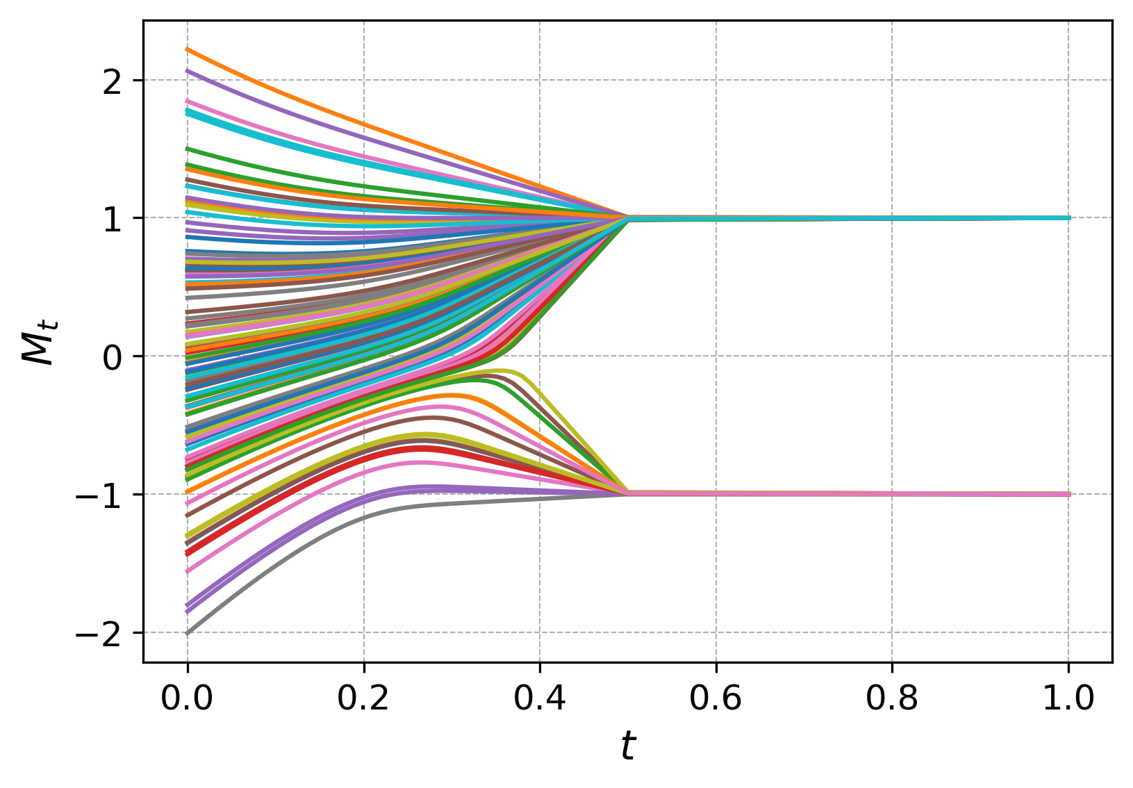
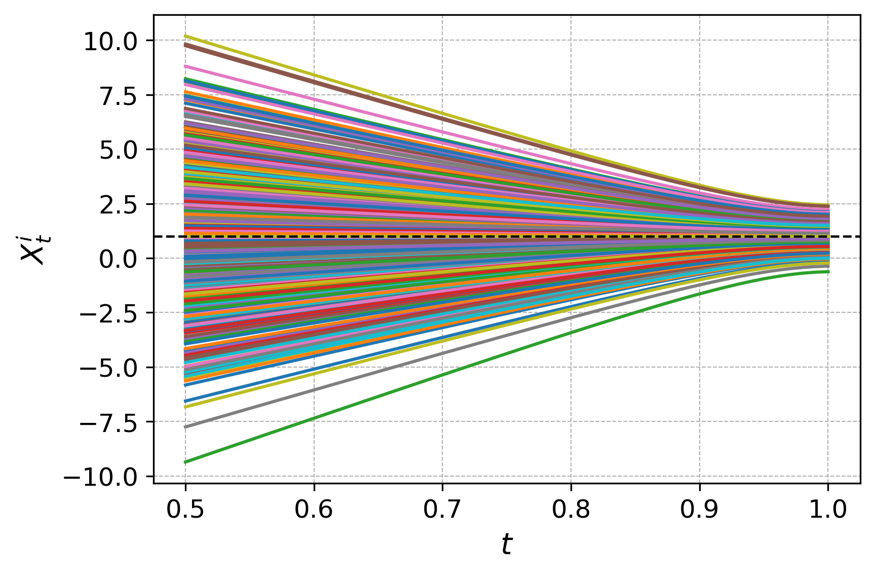
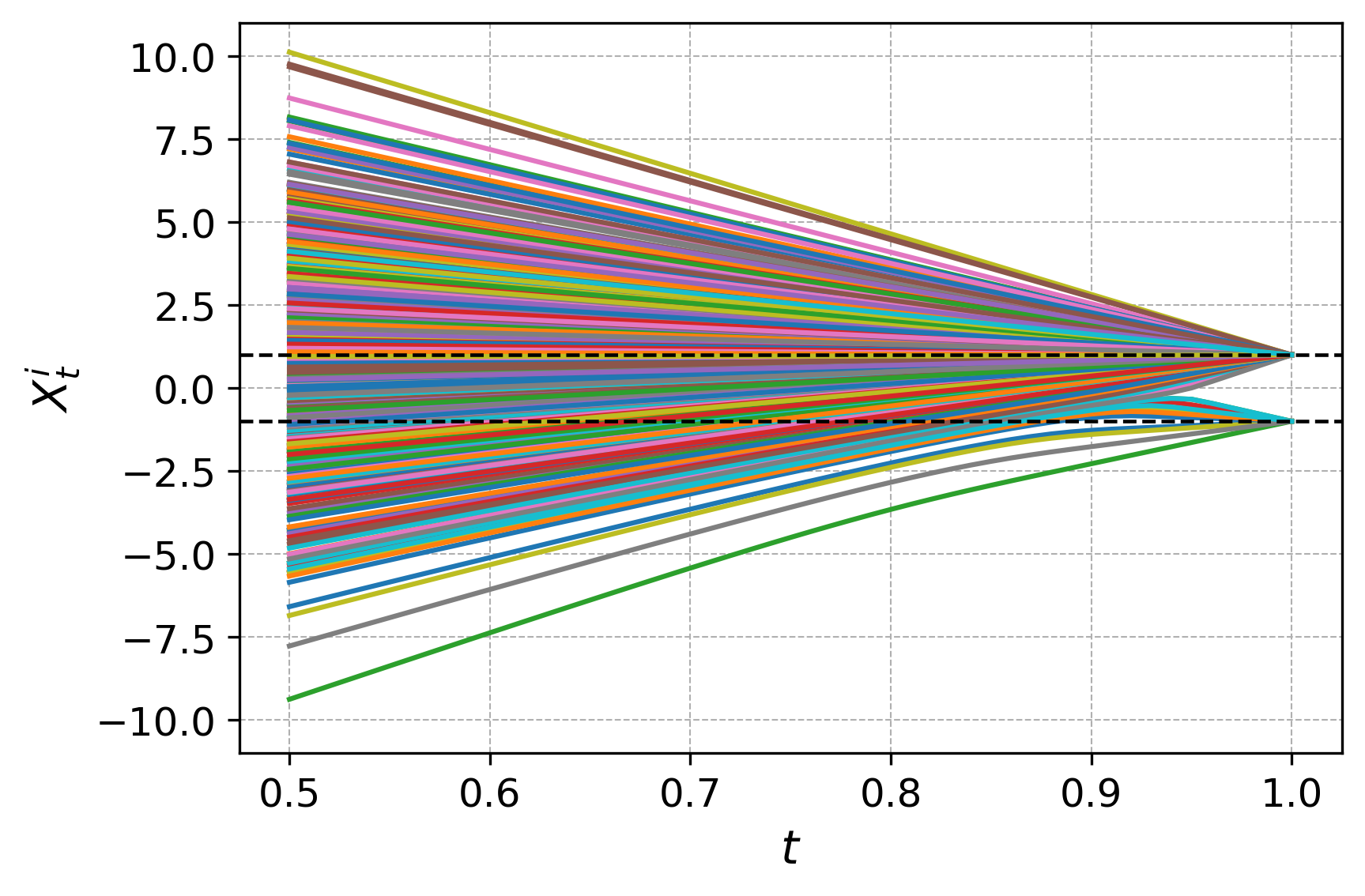
To confirm our results numerically, we run a discretized version of the probability flow ODE from equation (1) associated with the dilated VE interpolant. We work with dimension and discretization step Note the number of steps is significantly smaller than In Figure 2, we plot the magnetization for different realizations of . The plot confirms that gets determined in the first phase and remains fixed for the second phase We also plot in Figure 2 the coordinates of a single realization for the probability flow ODE associated with the dilated VE interpolant for both the GM and CW distribution, with the same realization of initial condition . We see that at the distributions look alike, but for close to they specialize to get samples from either the GM or CW distributions.
4.2 VP and VE on real data: CelebA
We showed earlier that, without time dilating, the high-level feature of the GM distribution given by the parameter is captured by the VE but not the VP interpolant, whereas the low-level feature given by is captured by the VP but not the VE interpolant. The theoretical analysis we gave is for the GM distribution under the probability flow ODE. However, the following experiment shows that this behavior is still present when working with real image distributions using the VP and VE SDE from [Song et al., 2021].
We use the dataset CelebA-HQ from [Karras et al., 2018] consisting of images of faces from celebrities. We use models pretrained on this dataset for the VP and VE SDEs from [Song et al., 2021]. Then, we generate images with the VP and VE SDEs and measure how well they reproduce the high- and low-level features of the dataset.
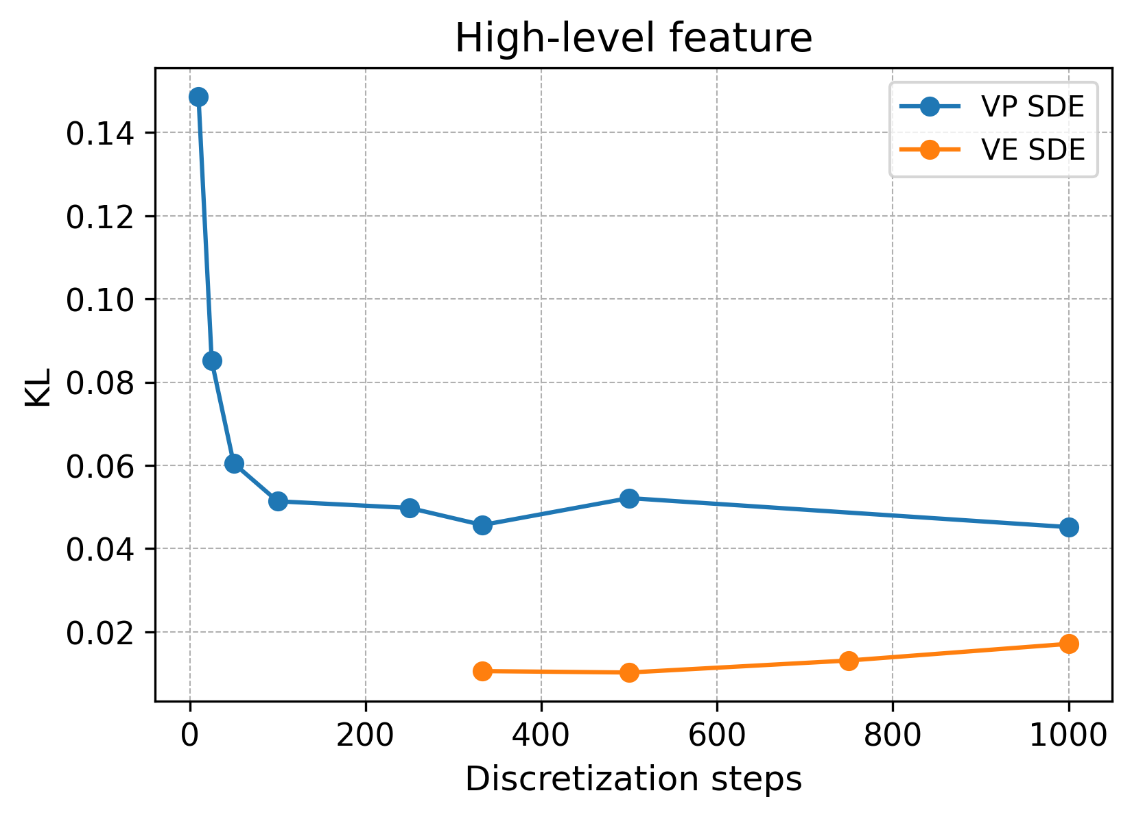
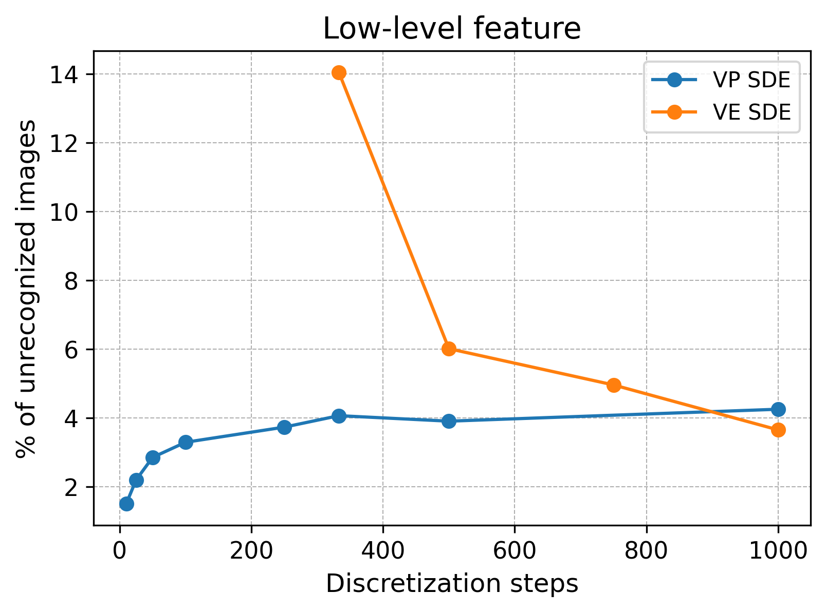
For the low-level feature, we use a neural network from the Deepface library [Serengil and Ozpinar, 2024] that detects whether there is a face in the generated image. For the high-level feature, we use another neural network that predicts the race of the person, and calculate the KL divergence between the race distribution of the original dataset and the race distribution of a set of images generated by the VP or VE SDEs. (See the appendix for details.)
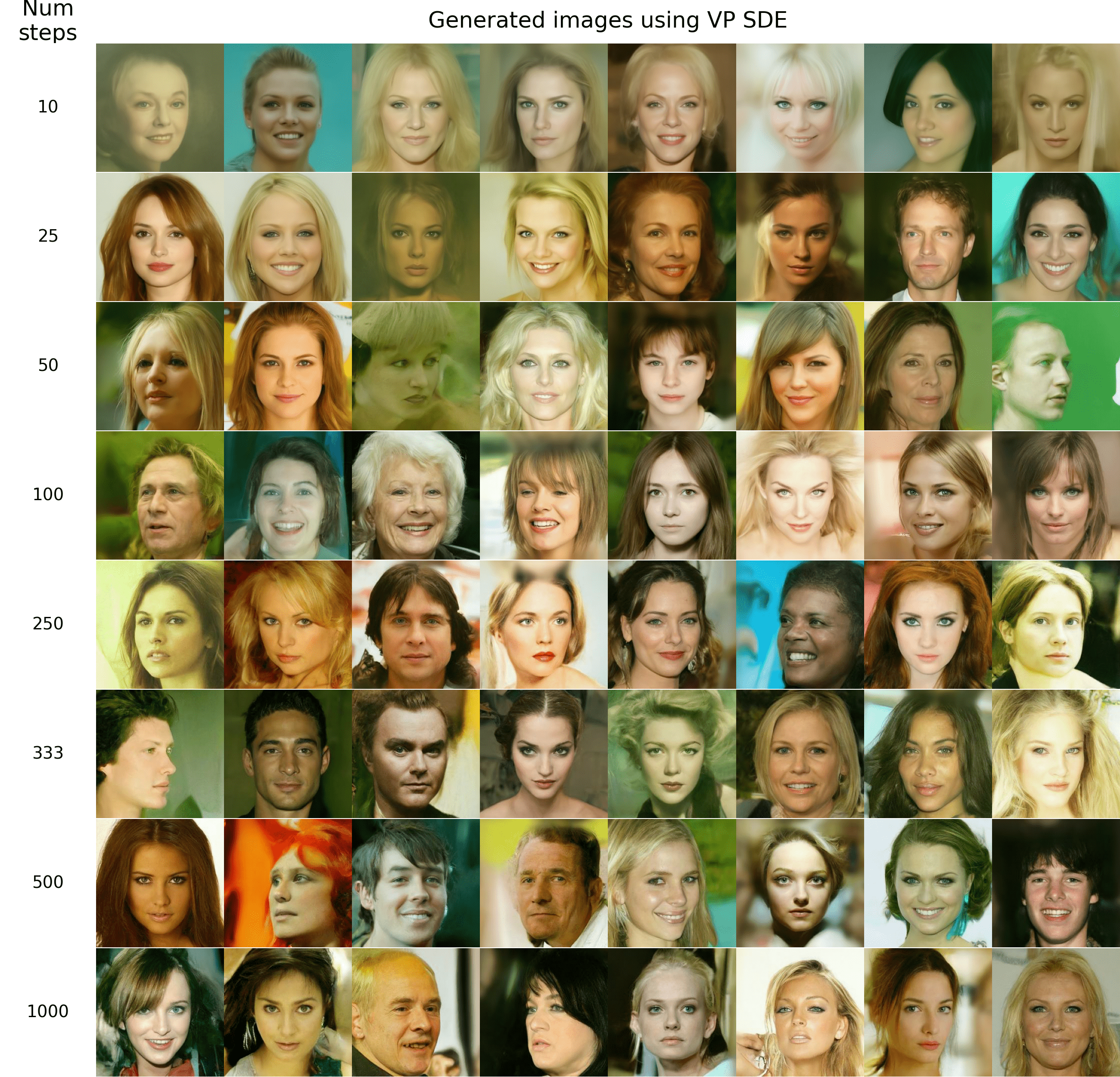
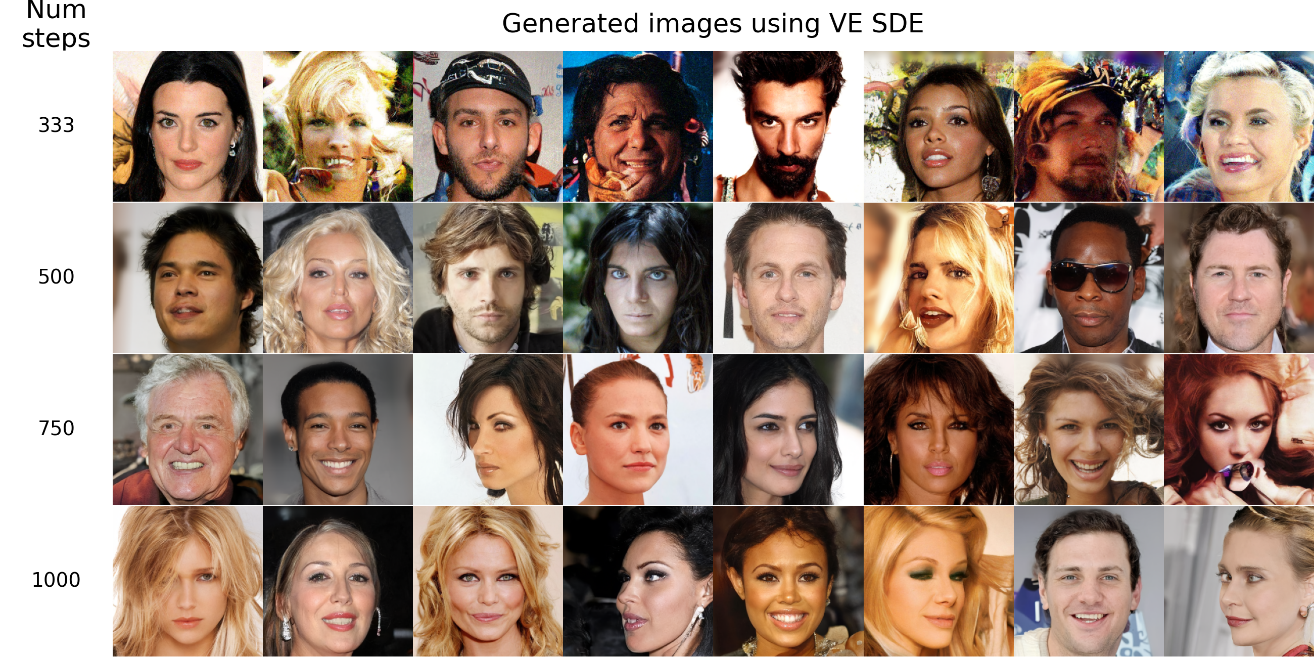
For a given number of discretization steps, we generate images with the VP and the VE SDEs using a uniform grid, and then measure the low- and high-level features as described before. The results are shown in Figure 3. We observe that increasing the number of discretization steps for the VP SDE makes it better at capturing high-level features but does not improve the low-level features. Conversely, taking more discretization steps for the VE SDE improves how well it reproduces low-level features, but does not improve the high-level features. This is further evidence that the VP SDE solves the low-level feature “by default” whereas the VE SDE solves the high-level feature “by default”.
References
- [Albergo et al., 2023] Albergo, M. S., Boffi, N. M., and Vanden-Eijnden, E. (2023). Stochastic interpolants: A unifying framework for flows and diffusions.
- [Albergo and Vanden-Eijnden, 2023] Albergo, M. S. and Vanden-Eijnden, E. (2023). Building normalizing flows with stochastic interpolants.
- [Behjoo and Chertkov, 2024] Behjoo, H. and Chertkov, M. (2024). U-turn diffusion.
- [Benton et al., 2024] Benton, J., Bortoli, V. D., Doucet, A., and Deligiannidis, G. (2024). Nearly -linear convergence bounds for diffusion models via stochastic localization.
- [Biroli et al., 2024] Biroli, G., Bonnaire, T., de Bortoli, V., and Mézard, M. (2024). Dynamical regimes of diffusion models.
- [Biroli and Mézard, 2023] Biroli, G. and Mézard, M. (2023). Generative diffusion in very large dimensions. Journal of Statistical Mechanics: Theory and Experiment, 2023(9):093402.
- [Chen et al., 2023] Chen, S., Chewi, S., Lee, H., Li, Y., Lu, J., and Salim, A. (2023). The probability flow ode is provably fast. In Oh, A., Naumann, T., Globerson, A., Saenko, K., Hardt, M., and Levine, S., editors, Advances in Neural Information Processing Systems, volume 36, pages 68552–68575. Curran Associates, Inc.
- [Esser et al., 2024] Esser, P., Kulal, S., Blattmann, A., Entezari, R., Müller, J., Saini, H., Levi, Y., Lorenz, D., Sauer, A., Boesel, F., Podell, D., Dockhorn, T., English, Z., Lacey, K., Goodwin, A., Marek, Y., and Rombach, R. (2024). Scaling rectified flow transformers for high-resolution image synthesis.
- [Gatmiry et al., 2024] Gatmiry, K., Kelner, J., and Lee, H. (2024). Learning mixtures of gaussians using diffusion models.
- [Google, 2021a] Google (2021a). Ddpm celeba-hq 256. https://huggingface.co/google/ddpm-celebahq-256.
- [Google, 2021b] Google (2021b). Ncsn++ celeba-hq 256. https://huggingface.co/google/ncsnpp-celebahq-256.
- [Ho et al., 2020] Ho, J., Jain, A., and Abbeel, P. (2020). Denoising diffusion probabilistic models. Advances in neural information processing systems, 33:6840–6851.
- [Karras et al., 2018] Karras, T., Aila, T., Laine, S., and Lehtinen, J. (2018). Progressive growing of gans for improved quality, stability, and variation.
- [Li and Chen, 2024] Li, M. and Chen, S. (2024). Critical windows: non-asymptotic theory for feature emergence in diffusion models.
- [Lipman et al., 2023] Lipman, Y., Chen, R. T. Q., Ben-Hamu, H., Nickel, M., and Le, M. (2023). Flow matching for generative modeling. In The Eleventh International Conference on Learning Representations.
- [Liu et al., 2022] Liu, X., Gong, C., and Liu, Q. (2022). Flow straight and fast: Learning to generate and transfer data with rectified flow.
- [Raya and Ambrogioni, 2023] Raya, G. and Ambrogioni, L. (2023). Spontaneous symmetry breaking in generative diffusion models.
- [Sclocchi et al., 2024] Sclocchi, A., Favero, A., and Wyart, M. (2024). A phase transition in diffusion models reveals the hierarchical nature of data.
- [Serengil and Ozpinar, 2024] Serengil, S. and Ozpinar, A. (2024). A benchmark of facial recognition pipelines and co-usability performances of modules. Journal of Information Technologies, 17(2):95–107.
- [Shah et al., 2023] Shah, K., Chen, S., and Klivans, A. (2023). Learning mixtures of gaussians using the ddpm objective.
- [Sohl-Dickstein et al., 2015] Sohl-Dickstein, J., Weiss, E., Maheswaranathan, N., and Ganguli, S. (2015). Deep unsupervised learning using nonequilibrium thermodynamics. In International conference on machine learning, pages 2256–2265. PMLR.
- [Song and Ermon, 2020] Song, Y. and Ermon, S. (2020). Improved techniques for training score-based generative models. In Larochelle, H., Ranzato, M., Hadsell, R., Balcan, M., and Lin, H., editors, Advances in Neural Information Processing Systems, volume 33, pages 12438–12448. Curran Associates, Inc.
- [Song et al., 2021] Song, Y., Sohl-Dickstein, J., Kingma, D. P., Kumar, A., Ermon, S., and Poole, B. (2021). Score-based generative modeling through stochastic differential equations.
Appendix A General results
We will need the following results that follow immediately from [Albergo et al., 2023] (Appendix A)
Lemma 2.
Let and . Then the law of the interpolant coincides with the law of the solution of the probability flow ODE
| (11) |
where is such that
Lemma 3.
Let and Then the law of the interpolant coincides with the law of the solution of the probability flow ODE
| (12) |
Lemma 4.
Let and Then the law of the interpolant coincides with the law of the solution of the probability flow ODE
| (13) |
where is such that
Lemma 5.
Let and Then the law of the interpolant coincides with the law of the solution of the probability flow ODE
| (14) |
where and fulfill
Appendix B Non-dilated interpolants fail at capturing either or for the GM
In this section we prove Proposition 1 and 2 from the main text, showing that without time-dilation, the VP and VE interpolant fail at either capturing or
Proof of Proposition 1.
(VP does not capture ) Consider the variance preserving interpolant with and Let be the solution of the probability flow ODE associated with given by Lemma 2. If we let we have for
| (15) |
with
For , we get that for large, since
| (16) |
Fix positive. If we run this equation from til the sign of will be preserved. This follows because since for means that whenever the second term in the RHS of (16) will dominate implying that
For we have
| (17) |
If we integrate this ODE with a step of size we get
This means that Since after this step the sign of will be preserved, we have that as
-
•
all samples will go to the mode.
-
•
half of the samples will go to and half to
-
•
all samples will go to the mode.
(VP captures ) Let We note the problem is symmetric in the orthogonal complement of so we expect to be the right object to look at. We have again from Lemma 2 that
| (18) |
We note that for any and discretization step size we have that will remain Gaussian. We then have
To determine we look at one coordinate and note that the resulting velocity field is independent of . Also, Lemma 3 shows that this is the -dimensional velocity field corresponding to the interpolant that transports to so we are done. ∎
Proof of Proposition 2.
(VE captures ) Let be the variance exploding interpolant with and Let be the solution of the probability flow ODE associated with given by Lemma 2. For we have
| (19) |
Taking the limit of this equation gives for
| (20) |
Hence we get a well-defined equation for the magnetization. Define the speciation time as the time in the generative process after which the mode of the samples is determined. Since determines the mode of the samples, and we obtained a -independent limiting equation for we get that as to Moreover, from Lemma 2 we know that the ODE for from equation (20) corresponds to the 1-dimensional velocity field that transports to
(VE does not capture .) We have
| (21) |
As in the proof of Proposition 1, we see that is Gaussian for any and Let be an orthonormal basis of the complement of Then for with we have
| (22) |
In the limit, we get
| (23) |
From Lemma 3 we know that this ODE transports to
∎
Appendix C Speciation time for the VP interpolant
In this section, we state and prove Proposition 3, showing that without time dilating, the VP interpolant has a speciation time that goes to zero as goes to infinity.
Proposition 3.
Consider the variance preserving interpolant where and and let be its associated probability flow ODE from equation (1) in the main text. Then, the speciation time (i.e. the time in the generative process after which the mode of the samples is determined) goes to zero as goes to infinity. In particular, the interpolant has speciation time
Proof.
We have from Lemma 2 that fulfills the ODE
| (24) |
Let We then have
| (25) |
where and Let us calculate the time where the terms and are of the same order. Since and are we are interested in finding such that , or equivalently Since and are independent of we get
| (26) |
We have for
| (27) |
and for
| (28) |
This means there is a transition in what term dominates in at This will imply, as formalized below, that each sample will speciate to one of the two modes for and it will remain in that mode for
Take We have by equation (27) that This means we can Taylor expand the term in to get
| (31) |
This is a quadratic well shifted away from the origin which will generate the asymmetry in the relative weights of the modes.
Take We have by equation (28) that since either and then or and then implies meaning that This means we can approximate (30) as follows
| (32) |
This is a symmetric double well structure. Under this potential, the mode that each sample will belong to is determined since the beginning. The relative asymmetry of the modes given by (which is a function of ) does not appear in this potential anymore.
We conclude that the speciation time In particular, if and we get that ∎
Proposition 4.
Let be obtained from the probability flow ODE from equation (1) in the main text associated with the VP interpolant where and Consider running this ODE with a uniform grid with step size Let Then
where
Proof.
We proceed similarly to the proof of Proposition 1. Let then we have for
| (33) |
with
For with positive integer, we get that goes to infinity as grows. This means that for large
| (34) |
Fix with positive integer again. If we run this equation from til the sign of will be preserved. This follows because whenever the second term in the RHS of (34) will dominate implying that
For we have
| (35) |
If we integrate this ODE with step size we get
This means that Since after this step the sign of will be preserved, we have that as
-
•
all samples will go to the mode.
-
•
half of the samples will go to and half to
-
•
all samples will go to the mode.
∎
Appendix D Dilated interpolants capture and for the GM
In this section, we prove Theorems 1 and 2 from the main text which show that the dilated VP and VE interpolant can recover and when time-dilated.
Proof of Theorem 1.
Consider the dilated variance preserving interpolant where and is given in equation (4) in the main text. Plugging in and into the velocity field given by Lemma 2 yields
| (36) |
First phase. For we have Plugging in into equation (36) gives
| (37) |
We then have with
| (38) |
Taking yields the limiting ODE for the in the first phase. By reparameterizing time with we get from Lemma 4 (with ) that this the -dimensional velocity field associated to the interpolant that transports at to at
Let We have from equation (36)
| (39) |
Since this is a linear ODE with initial condition Gaussian, we have
| (40) |
for any and Further, using equation (39) with gives meaning that for
| (41) |
Second phase. For we have Using equation (114) again gives
| (42) |
Writing this implies
| (43) |
From equation 38 of the first phase, we have that for finite and discretizing with a step size of we get
| (44) |
where and the term goes to zero as goes to zero independently of since this error only comes from discretizing the -independent ODE with
At the argument of the is Assume takes value on the mode. For large enough and small enough (independently of ) we have that . We also have that and hence where both inequalities hold with probability going to as goes to infinity. This means we can approximate the ODE for for as
| (45) |
We note that this remains valid for since under the approximation we used in equation (45), we have that is increasing. Indeed, whenever the second term in the RHS of (45) will dominate. If takes value on the mode instead, an analogous argument shows that (45) is also valid in that case.
We then use this approximation in the ODEs for to get for
| (46) |
where This yields the limiting ODE for in the theorem statement. We recall that from the analysis of the first phase (after taking the limit first on and then on ) we got
| (47) |
We argued above that the sign of will be preserved for with probability going to as tends to This means that
| (48) |
where is such that
Let and note that
| (49) |
Since this is a linear ODE from a Gaussian initial condition, we have
| (50) |
Under the change of variables the equation (49) for becomes
| (51) |
By taking one coordinate of we get from Lemma 3 that this is the velocity field associated with the interpolant where is transported to For fixed the interpolant has variance as claimed. ∎
We now turn to the proof of Theorem 2 proving that the dilated variance exploding interpolant yields correct estimation of and
Proof of Theorem 2.
Consider the variance exploding interpolant with the time dilation given by equation (5) in the main text. Plugging in and into the velocity field given by Lemma 2 yields
| (52) |
| (53) |
where and
First phase. We consider where gives
| (54) |
We hence get a well-defined equation for the magnetization. In fact, by reparameterizing time with we get from Lemma 2 that this the -dimensional velocity field that transports at to at
We let and note that equation (52) gives
| (55) |
Since this is a linear ODE with Gaussian initial condition, will be Gaussian for every even for nonzero Let us determine its covariance. We decompose as Plugging in into equation (52) gives
| (56) |
Taylor expanding the RHS in powers of and matching terms of order gives
| (57) |
with This means that for we have Matching terms of constant order
| (58) | ||||
| (59) |
From here we conclude that We then have
| (60) |
where
Second phase. We now consider Using the definition of , we get from equation (52) that for large,
| (61) |
In particular,
| (62) |
Since is either or we see that it will remain constant in the second phase. On the other hand, we have
| (63) |
Solving explicitly gives for
| (64) |
From the analysis of the first phase, we know that
| (65) |
where We hence get for that
| (66) |
where ∎
Appendix E Dilated interpolants capture both phases for CW model
In this section, we prove Theorem 3 from the main text, showing that the dilated VE interpolant captures both phases for the CW distribution. We also state and prove Theorem 4, proving that the VP interpolant captures both phases. We will need the following lemma
Lemma 6.
For all , the law of the interpolant is the same as the law of the solution to the probability flow ODE
| (67) |
Proof.
This follows from combining the equations
| (68) | |||
| (69) |
where the second equation follows from Theorem 2.6 in [Albergo et al., 2023] ∎
Proof of Theorem 3.
We write explicitly as
| (70) |
where
| (71) |
First phase. For we have
| (72) | ||||
| (73) |
where and we linearized the to get the second equation. These approximations require to be small. We note that
| (74) |
Since for we have , then Hence regulates how good these approximations are, so that for large enough, they are valid.
Combining the two approximations and using that gives
| (75) |
Lemma 6 tells us that the law of the interpolant is the same as that of the solution to the ODE
| (76) |
Putting this together, and using gives
| (77) |
with Using the definition of we get
| (78) |
We hence get a well-defined equation for the magnetization. In fact, after taking the limits by reparameterizing time with we get from Lemma 2 that this the -dimensional velocity field that transports at to at as desired.
Now let and write
| (79) |
Taylor expanding the RHS in powers of and matching terms of order gives
| (80) |
where Hence for we have We now match terms of constant order in (79) to get
| (81) | ||||
| (82) |
We get . Fix Since we then have for that
Second phase. Consider Using Lemma 6 again, we get that the law of is the same as that of which solves the ODE
| (83) |
Using the definition of
| (84) |
For large enough, we can approximate for as
We note that and recall from the analysis of the first phase that under the appropiate limits we get In particular, we have that for large, either or We will approximate the ODEs under the assumption that this holds for i.e., either or for all The resulting ODEs will allow us to compute the value for and check that indeed either or for showing self-consistency and justifying the assumption. We first note that our assumption on means that we can approximate
| (85) |
where is applied elementwise. Combining this with (84) gives
| (86) |
Fix a coordinate and without loss of generality, consider We have
| (87) |
From our analysis of the first phase, we have that where Under the change of variables equation (87) becomes
| (88) |
In the limit of we get from Lemma 5 that this velocity field transports with to In particular, we know that for If we instead had we would have the same results except that
We will now argue that will remain fixed for Again without loss of generality, we take and we get the evolution of the in equation (112). Since the are iid at and evolve identically and independently, we get that by the law of large numbers as
Similarly, we get that as
| (89) |
Hence, using that for with we have
| (90) |
We claim that from where it follows immediately that remains constant for To prove the claim note that since it suffices to show
| (91) |
We have
| (92) | ||||
| (93) | ||||
| (94) | ||||
| (95) |
where in the last equality we changed variables in the first term of the integral and in the second term.
Since yields
we then get by rearranging that
which implies that the integrand of equation (95) is zero, giving the desired result.
We now check the self-consistency of the assumption that either or Using the definition of and and the fact that the evolve independently and identically, we get by the law of large numbers that
| (96) | ||||
| (97) |
This means that to leading order in we have We then have using the fact that evolve independently
| (98) |
A similar computation to the one used to prove equation (91) gives
| (99) |
where we evolve taking This yields as desired. If we had taken we would have gotten ∎
Theorem 4 (Dilated VP captures both features for CW model).
Let be obtained from the probability flow ODE associated with the dilated VP interpolant for the CW distribution discretized with a uniform grid with step size Let
First phase: For we have that
fulfills
with such that This implies
In addition, for we have for
Second phase: For we have that
fulfills, for , the ODE
Moreover, for any coordinate we have that
satisfies the ODE for
with the intial condition This equation implies that
Proof of Theorem 4.
First phase. For we have
| (102) | ||||
| (103) |
where and we linearized the to get the second equation. These approximations are valid since in the first phase is small. Combining the two approximations gives
| (104) |
Lemma 6 tells us that the law of the interpolant is the same as that of the solution to the ODE
| (105) |
Combining the last two equations with gives us the ODE
| (106) |
Writing gives the induced equation
| (107) |
Taking yields the limiting ODE for the in the first phase. By reparameterizing time with we get from Lemma 4 that this the -dimensional velocity field associated to the interpolant that transports at to at Now fix with Let From equation (106), we get that for
This means that as claimed.
Second phase. For we have using Lemma 6 and the definition of
| (108) |
We will approximate based on the fact that either or To see this, write where and and note that at we have
where This means that for large enough, we can approximate as
We note that In particular, we have that with probability that goes to as goes to infinity, either or We will approximate the ODEs under the assumption that this holds for i.e., either or for all Similarly to the proof of Theorem 3, one can use the resulting equations to show self-consistency of this assumption.
Our assumption on implies that we can approximate
| (109) |
where is applied elementwise. Combining this with (108) gives
| (110) |
From our analysis of the first phase, we note that where Let us assume without loss of generality that and fix a coordinate
| (111) |
Under the change of variables we get that the ODE becomes
| (112) |
In the limit of we get from Lemma 5 that this velocity field transports to using the interpolant
From the equation for we deduce
| (113) |
A similar computation to the one in the proof of Theorem 3 yields giving the desired equation for
∎
Appendix F Dilated VP captures and
We proved in Theorem 1 from the main text that taking the VP interpolant and using the dilation from equation (4) in the main text leads to correct estimation for both and for the GM distribution. We now show that the same time dilation leads to correct estimation if we instead use the interpolant The analysis of the first phase mimics that of Theorem 1, since in the first phase. The second phases for these two interpolants are also similar, but the details of the ODEs change.
Theorem 5.
Let be obtained from the probability flow ODE associated with the dilated VP interpolant discretized with a uniform grid with step size Then
where is characterized as follows:
First phase: For we have
In addition
fulfills
where is such that This implies
Second phase: For we have
In addition
fulfills, for , the ODE
and satisfies
where is such that
Proof.
Consider the dilated variance preserving interpolant where and is given in equation (4) in the main text. Plugging in and into the velocity field given by Lemma 2 yields
| (114) |
First phase. For we have Plugging in into equation (114) gives
| (115) |
The remaining of the analysis of the first phase to yield the desired results is almost identical to what we did in the proof of Theorem 1 and is omitted.
Second phase. For we have Using equation (114) again yields
| (116) |
Writing this implies
| (117) |
From the analysis of the first phase (see equation (38) in the proof of Theorem 1), we have that for finite and discretizing with step size
| (118) |
where and the term goes to zero as goes to zero independently of since this error only comes from discretizing the -independent ODE with
At the argument of the is Assume takes value on the mode. For large enough and small enough (independently of ) we have that . We also have that and hence where both inequalities hold with probability going to as goes to infinity. This means we can approximate the ODE for for as
| (119) |
We note that this remains valid for since under the approximation we used in equation (119), we have that is increasing. Indeed, whenever the second term in the RHS of (119) will dominate. If takes value on the mode instead, an analogous argument shows that (119) is also valid in that case.
We then use this approximation in the ODEs for to get for
| (120) |
where This yields the limiting ODE for in the theorem statement. We recall that from the analysis of the first phase (after taking the limit first on and then on ) we got
| (121) |
We argued above that the sign of will be preserved for with probability going to as tends to This means that
| (122) |
where is such that
Let and note that
| (123) |
Since this is a linear ODE from a Gaussian initial condition, we have
| (124) |
Under the change of variables the equation (123) for becomes
| (125) |
By taking one coordinate of we get from Lemma 3 that this is the velocity field associated with the interpolant where is transported to For fixed the interpolant has variance as claimed. ∎
Appendix G Connection with the sub-VP SDE.
Similarly to the connection described in Section 3.3 between our VP interpolant and the VP SDE from [Song et al., 2021], we note that the sub-VP SDE from [Song et al., 2021] corresponds to the interpolant with as in Section 3.3. Hence, the sub-VP SDE corresponds exactly to a time-dilation of the VP interpolant we analyze in Theorem 1.
Appendix H Details for the CelebA experiment
As mentioned in the main text, we use pretrained models for the VP and VE SDEs from [Song et al., 2021]. We use pretrained models on the CelebA-HQ dataset [Karras et al., 2018]. These models are available publicly on the HuggingFace library for the VP SDE [Google, 2021a] and for the VE SDE [Google, 2021b]. We note that for the VP SDE we actually use the DDPM model from [Ho et al., 2020] which was later shown to correspond to a particular discretization of Song et al’s VP SDE (see Appendix E in [Song et al., 2021].)
We then generate samples running the VP or VE SDEs with different number of discretization steps with a uniform grid. For a given number of discretization steps, we generate samples and then use the DeepFace library from [Serengil and Ozpinar, 2024] to detect whether there is a face in the generated image. This measures the low-level feature of the image. For the high-level feature, when the DeepFace library does detect a face, it tries to predict the race of the generated face, giving one of the following races: Asian, Black, Indian, Latino/Hispanic, Middle Eastern, White. Given the predicted races in the samples were a face was detected among the , we calculate an empirical distribution supported on points. We also calculated the race distribution on the original CelebA-HQ dataset which has real images. We then compute the KL Divergence between the distribution on races of the generated images and the images in the dataset.
A technical detail is that the DDPM implementation from [Google, 2021a] can only handle a number of discretization steps that is of the form where is an integer. For the VP SDE, we use one of the following options for the number of discretization steps. For the VE SDE, we instead use one of A smaller number of discretization steps for the VE SDE leads to images that are too low-quality for our purposes.
As a sanity check, we include non-cherry-picked samples from the VP SDE in Figure 4 and from the VE SDE in Figure 5. We confirm that diversity increases for the images generated by the VP SDE as the number of steps grows, whereas quality increases for the images generated by the VE SDE as we take larger number of steps.