Cyber-physical Defense for Heterogeneous Multi-agent Systems Against Exponentially Unbounded Attacks on Signed Digraphs

Abstract

Cyber-physical systems (CPSs) are subjected to attacks on both cyber and physical spaces. In reality, the attackers could launch exponentially unbounded false data injection (EU-FDI) attacks, which are more destructive and could lead to the system’s collapse or instability. Existing literature generally addresses bounded attack signals and/or bounded-first-order-derivative attack signals, which exposes the CPSs to significant threats. In contrast, this paper proposes a fully-distributed attack-resilient bi-layer defense framework to address the bipartite output containment problem for heterogeneous multi-agent systems on signed digraphs, in the presence of EU-FDI attacks on both cyber-physical layer (CPL) and observer layer (OL). First, we design attack-resilient dynamic compensators that utilize data communicated on the OL to estimate the convex combinations of the states and negative states of the leaders. The attack-resilient compensators address the EU-FDI attacks on the OL and guarantee the uniformly ultimately bounded (UUB) estimation of the leaders’ states. Then, by using the compensators’ states, fully-distributed attack-resilient controllers are designed on the CPL to further address the EU-FDI attacks on the actuators. Rigorous mathematical proof based on Lyapunov stability analysis is provided, establishing the theoretical soundness of the proposed bi-layer resilient defense framework, by preserving the UUB consensus and stability against EU-FDI attacks on both CPL and OL. Finally, a comparative case study for heterogeneous multi-agent systems validate the enhanced resilience of the proposed defense strategies.

I Introduction

In recent decades, Multi-Agent Systems (MASs) have seen substantial advancements and have become a key research area in the system and control community due to their promising applications [1, 2, 3, 4]. The dynamics of interactions in MASs are crucial for understanding and optimizing system performance. Significant progress has been made in achieving consensus and other collective behaviors in MASs across various network types, such as fixed, time-varying, and leader-follower networks, as demonstrated by [5]. Despite these advancements, cooperative control within MASs remains an area that deserves more in-depth exploration [6]. Understanding cooperative control is essential as it directly affects the efficiency and effectiveness of collaborative tasks in complex environments. In the systems of most of the studies, the interaction topology is typically represented by an unsigned graph, assuming that the interaction weights among the agents are positive. This representation, while effective in a broad sense, may not always encapsulate the complexities of certain real-world systems. In light of this, it is crucial to delve into the nuances of cooperative control in MASs, examining how this approach can be adapted or enhanced to better reflect the complexities of real-world scenarios. Take, for instance, social networks or political opinion dynamics within two-party systems [7], where individuals’ ideas or views do not uniformly align. A similar scenario is observed in antagonistic robotic networks [8], gene transcriptional regulation biological network [9], and predator-prey interactions [10], etc., where agents exhibit both cooperative and antagonistic behaviors. When considering multiple leaders and followers in heterogeneous MASs that communicate on signed digraphs with both cooperative and antagonistic interactions, the classical bipartite consensus problems are transformed into bipartite output containment problems[11, 12].

The MASs are susceptible to cyber-physical attacks[13]. The existing literature has made strides in developing resilient control protocols to mitigate the impact of cyber-physical attacks. In [14], it is investigated that bipartite containment control in networked agents under denial-of-service attacks, employing dynamic signed digraphs to model variable communication links. In [15], it is addressed that bipartite containment control in nonlinear MASs with time-delayed states under impulsive False Data Injection (FDI) attacks, and with Markovian variations in communication topology. In [16], it is studied that dual-terminal dynamic event-triggered bipartite output containment control in heterogeneous linear MASs with actuator faults. The literature [17] introduces an innovative adaptive bipartite consensus tracking strategy for MASs under sensor deception attacks. In [18], it is explored that the design of bipartite formation containment tracking in heterogeneous MASs, considering external disturbances and inaccessible state vectors. In [19], it is investigated that adaptive bipartite output containment in heterogeneous MASs through a signed graph and a protocol with a distributed observer, addressing unmeasurable yet bounded inputs in leader dynamics. However, the aforementioned literature has only dealt with bounded disturbances or bounded attack signals. In reality, adversaries can inject any time-varying signal into systems via software, CPU, DSP, or similar platforms. The attacker could launch unbounded attack signals which are more destructive and could lead to the system’s collapse or instability. While [20] address unbounded attacks, it requires that the first-order time derivatives of the attacks be bounded. In addition, an observer design is generally needed to address the output regulation problem for heterogeneous MASs by estimating the leaders’ states. However, existing literature on heterogeneous MASs typically assumes that the observers remain intact against cyber-attacks, which is not practical.

In contrast, the fast-growing Exponentially Unbounded False Data Injection (EU-FDI) attacks are considered in the bipartite output containment problem for heterogeneous MASs in this paper. Moreover, a bi-layer defense architecture is developed for heterogeneous MASs, consisting of the Cyber-Physical Layer (CPL) and the Observer Layer (OL). The system resilience against EU-FDI attacks on both layers is investigated, which is more practical and challenging. The main contributions of this paper are threefold:

• A general Attack-resilient Bipartite Output Containment (ARBOC) problem is first formulated, considering both cooperative and antagonistic interactions among agents, removing the assumption that the edge weights have the same sign. To the best of the authors’ knowledge, the rigorous mathematical proof is provided for the first time, which asserts that the ARBOC problem is solved by ensuring that the neighborhood bipartite output containment error is uniformly ultimately bounded (UUB).

• While the majority of the literature addressing the output regulation problem for heterogeneous MASs assumes that the observers employed be uncompromised to cyber-physical attacks, we remove this strict limitation by developing a fully-distributed bi-layer defense framework, which addresses attacks on both CPL and OL. Moreover, the proposed resilient control protocols can effectively handle EU-FDI attacks on both layers. This goes beyond the strict constraint of bounded-first-order-time-derivative attack signals [20]. Hence, this advancement enriches the capabilities of bipartite output containment control systems in countering more general cyber-physical threats in adversarial environments.

• A rigorous mathematical proof using Lyapunov stability analysis certifies the UUB consensus and stability of the heterogeneous MASs in the face of EU-FDI attacks, establishing the theoretical soundness of the proposed method. Comparative simulation case studies validate the effectiveness of the proposed bi-layer defense strategies.

The remainder of this paper is structured as follows: Section II outlines the preliminaries and formulates the problem. Section III presents the design of a fully-distributed attack-resilient defense strategies. Section IV provides validation of the proposed defense strategies through numerical simulations. Finally, Section V conclusions the paper.

II Preliminaries and Problem Formulation

In this section, the preliminaries on graph theory and notations are first given, and then the ARBOC problem is formulated.

II-A Preliminaries on Graph Theory and Notations

Consider a group of $N+M$ agents on a signed communication digraph $\mathscr{G}$, consisting of $N$ followers and $M$ leaders. Leaders are characterized by the absence of incoming edges, thus they operate autonomously. In contrast, followers obtain and process information from their adjacent agents. Denote the follower set and the leader set as $\mathscr{F}=\{v_{1},v_{2},\ldots,v_{N}\}\quad\text{and}\quad\mathscr{L}=\{v_{N+1},v_{N+2},\ldots,v_{N+M}\}$ respectively. The interactions among the followers are represented by ${\mathscr{G}_{f}}=(\mathcal{V},\mathcal{E},\mathcal{A})$ with a nonempty finite set of nodes $\mathcal{V}$, a set of edges $\mathcal{E}\subset\mathcal{V}\times\mathcal{V}$, and $\mathcal{A}=[a_{ij}]\in\mathbb{R}^{N\times N}$ is the adjacency matrix, where ${a_{ij}}$ is the weight of edge $({v_{j}},{v_{i}})$, with $a_{ij}\neq 0$ if $(v_{j},v_{i})\in\mathcal{E}$; otherwise, $a_{ij}=0$. It is assumed there are no repeated edges and no self-loops, i.e., $a_{ii}=0$, $\forall i$. A sequence of successive edges in the form $\{({v_{i}},{v_{k}}),({v_{k}},{v_{l}}),\ldots,({v_{m}},{v_{j}})\}$ is a directed path from node $i$ to node $j$. The matrix $\mathcal{G}_{r}=\operatorname{diag}(g_{ir})\in\mathbb{R}^{N\times N}$, with $i\in\mathscr{F}$ and $r\in\mathscr{L}$, represents the diagonal matrix of pinning gains from the $r$th leader to each follower. $g_{ir}\neq 0$ if a link from the $r$th leader to the $i$th follower exists; otherwise, $g_{ir}=0$. It is assumed that the signed digraph $\mathscr{G}$ is time-invariant, i.e., both $\mathcal{A}$ and $\mathcal{G}_{r}$ are constant.

In this paper, we use the features of global graph topology matrices of two correlated digraphs:

• For the non-negative digraph $\bar{\mathscr{G}}$, we define the adjacency matrix as $\bar{\mathcal{A}}=[|{a}_{ij}|]\in\mathbb{R}^{N\times N}$ and the pinning gain matrix as $\bar{{\mathcal{G}}}_{k}=\operatorname{diag}(|g_{ir}|)\in\mathbb{R}^{N\times N}$. The conventional Laplacian matrix is defined as

  $$\bar{\mathcal{L}}=\bar{\mathcal{D}}-\bar{\mathcal{A}}=\operatorname{diag}\left(\sum_{j\in\mathscr{F}}|a_{ij}|\right)-[|a_{ij}|].$$

1. For the signed digraph $\mathscr{G}$, consider the adjacency matrix $\mathcal{A}=[a_{ij}]\in\mathbb{R}^{N\times N}$ and the matrix of pinning gains $\mathcal{G}_{r}=\operatorname{diag}(g_{ir})\in\mathbb{R}^{N\times N}$. The signed Laplacian matrix is defined as

   $$\mathcal{L}^{s}=\bar{\mathcal{D}}-\mathcal{A}=\operatorname{diag}\left(\sum_{j\in\mathscr{F}}|a_{ij}|\right)-[a_{ij}].$$

Throughout this study, we adopt the following notations:

• ${I_{N}}\in{\mathbb{R}^{N\times N}}$ is the identity matrix.

• ${{\mathbf{1}}_{N}}\in{\mathbb{R}^{N}}$ and ${{\mathbf{0}}_{N}}\in{\mathbb{R}^{N}}$ are column vectors with all elements of one and zero, respectively.

• The Kronecker product is represented by $\otimes$.

• The operator $\operatorname{diag}(\cdot)$ is used to form a block diagonal matrix from its argument.

• ${\sigma_{\min}}(X)$, ${\sigma_{\max}}(X)$, and $\sigma(X)$ are the minimum singular value, the maximum singular value, and the spectrum of matrix $X$, respectively.

• $\left\|\cdot\right\|$ is the Euclidean norm of a vector.

II-B Problem Formulation

Consider a group of $N$ followers with the following general high-order linear heterogeneous dynamics

$$\begin{gathered}\left\{\begin{gathered}{{\dot{x}}_{i}}={A_{i}}{x_{i}}+{B_{i}}{u^{c}_{i}},\hfill\\ {y_{i}}={C_{i}}{x_{i}},\hfill\end{gathered}\right.\quad i\in\mathscr{F}\hfill\end{gathered}$$ (1)

where ${x_{i}}\in\mathbb{R}^{n_{i}}$ and ${y_{i}}\in{\mathbb{R}^{z}}$ are the state and output of the $i$th follower, respectively. ${u_{i}^{c}}$$\in{\mathbb{R}^{m_{i}}}$ is the compromised input of the $i^{th}$ follower. The local input is under unknown and unbounded actuator attack described by

$${u_{i}^{c}}={u_{i}}+{\gamma^{a}_{i}},$$ (2)

where ${u_{i}}\in\mathbb{R}^{m_{i}}$ is the intact control input and ${\gamma^{a}_{i}}\in\mathbb{R}^{n_{i}}$ is of class $C^{1}$ [21]that represents the EU-FDI attack signal injected to the $i^{th}$ follower.

The $M$ leaders with the following dynamics can be viewed as command generators that generate the desired trajectories

$$\begin{gathered}\left\{\begin{gathered}{{\dot{x}}_{r}}=S{x_{r}},\hfill\\ {y_{r}}=R{x_{r}},\hfill\\ \end{gathered}\right.\quad r\in\mathscr{L}\hfill\\ \end{gathered}$$ (3)

where ${x_{r}}\in{\mathbb{R}^{l}}$ and ${y_{r}}\in{\mathbb{R}^{z}}$ are the state and output of the $r$th leader, respectively. Noting that $({A_{i}},{B_{i}},{C_{i}})$ and $(S,R)$ may have different system matrices and state dimensions, and hence are heterogeneous.

Definition 1 (Structurally balanced[22]).

The signed subgraph ${\mathscr{G}_{f}}$ is said structurally balanced if it admits a bipartition of the nodes ${\mathcal{V}_{1}}$, ${\mathcal{V}_{2}}$, ${\mathcal{V}_{1}}\cup{\mathcal{V}_{2}}=\mathcal{V}$, ${\mathcal{V}_{1}}\cap{\mathcal{V}_{2}}=0$, such that ${a_{ij}}\geqslant 0,\forall{v_{i}},{v_{j}}\in{\mathcal{V}_{q}},\left({q\in\left\{{1,2}\right\}}\right)$, and ${a_{ij}}\leqslant 0,\forall{v_{i}}\in{\mathcal{V}_{q}},{v_{j}}\in{\mathcal{V}_{r}},q\neq r,\left({q,r\in\left\{{1,2}\right\}}\right)$. It is said structurally unbalanced otherwise.

Definition 2 (Convex hull[23]).

A set $\mathfrak{C}\subseteq{\mathbb{R}^{n}}$ is convex if $({1-\lambda})x+\lambda y\in\mathfrak{C}$, for any $x,y\in\mathfrak{C}$ and any $\lambda\in\left[{0,1}\right]$. Let ${Y_{\mathscr{L}}}=\left\{{{y_{N+1}},-{y_{N+1}},{y_{N+2}},-{y_{N+2}},...,{y_{N+M}},-{y_{N+M}}}\right\}$ be the set of the outputs and the negative outputs of the leaders. The convex hull ${\text{Co}}({Y_{\mathscr{L}}})$ spanned by the outputs and the negative outputs of the leaders is the minimal convex set containing all points in ${Y_{\mathscr{L}}}$. That is, ${\text{Co}}({{Y_{\mathscr{L}}}})=\left\{{\left.{\sum_{r=N+1}^{N+M}{({a_{r}}{y_{r}}-{b_{r}}{y_{r}}})}\right|{a_{r}},{b_{r}}\geqslant 0,\sum_{r=N+1}^{N+M}{({a_{r}}+{b_{r}})}=1}\right\}$, where ${\sum_{r=N+1}^{N+M}{({a_{r}}{y_{r}}-{b_{r}}{y_{r}}})}$ is the convex combination of the outputs and the negative outputs of the leaders.

Definition 3 (Distance).

The distance from $x\in\mathbb{R}^{n}$ to the set $\mathcal{C}\in\mathbb{R}^{n}$ in the sense of Euclidean norm is denoted by $\operatorname{dist}(x,\mathcal{C})$, i.e., $\operatorname{dist}(x,\mathcal{C})=\inf_{y\in\mathcal{C}}\|x-y\|_{2}$.

Definition 4 (UUB[24]).

The signal $x(t)\in{\mathbb{R}^{n}}$ is said to be UUB with the ultimate bound $b$, if there exist positive constants $b$ and $c$, independent of ${t_{0}}\geqslant 0$, and for every $a\in\left({0,c}\right)$, there is $T=T\left({a,b}\right)\geqslant 0$, independent of $t_{0}$, such that

$$\left\|{x\left({{t_{0}}}\right)}\right\|\leqslant a\;\;\Rightarrow\;\;\left\|{x\left(t\right)}\right\|\leqslant b,\forall t\geqslant{t_{0}}+T$$ (4)

We have the following assumptions on the communication digraph and the MASs.

Assumption 1.

Each follower in the signed digraph ${\mathscr{G}}$, has a directed path from at least one leader.

Assumption 2.

$S$ has non-repeated eigenvalues on the imaginary axis.

Assumption 3.

The signed subdigraph ${\mathscr{G}_{f}}=(\mathcal{V},\mathcal{E},\mathcal{A})$ is structurally balanced.

Assumption 4.

$({A_{i}},{B_{i}})$ is stabilizable and $({A_{i}},{C_{i}})$ is detectable for each $i\in\mathscr{F}$.

Assumption 5.

$$\operatorname{rank}\left[{\begin{array}[]{*{20}{c}}{{A_{i}}-\lambda{I_{{n_{i}}}}}&{{B_{i}}}\\ {{C_{i}}}&0\end{array}}\right]={n_{i}}+z,\;\forall\lambda\in\sigma(S),\;i\in\mathscr{F}.$$ (5)

Remark 1.

Assumption 4[25] and Assumption 5 [26] are standard for output regulation of heterogeneous MASs. Assumption 2 is made to avoid the trivial case when $S$ has eigenvalues with negative real parts.

The following lemmas facilitate the stability analysis of the main result to be presented in the next section.

Lemma 1 ([22]).

Consider the signed subdigraph $\mathscr{G}_{f}$. We represent the set of signature matrix set as

$$\mathcal{Q}=\{\operatorname{diag}(\sigma_{i})\mid\sigma_{i}\in\{+1,-1\}\}.$$

$\mathscr{G}_{f}$ is called structurally balanced if and only if

1. The associated undirected graph $\mathscr{G}(\mathcal{A}_{u})$ is structurally balanced, where $\mathcal{A}_{u}=\frac{\mathcal{A}+\mathcal{A}^{T}}{2}$.

2. There exists a matrix $Q=Q^{T}=Q^{-1}\in\mathcal{Q}$, such that $\bar{\mathcal{A}}=[|a_{ij}|]=Q\mathcal{A}Q$.

Lemma 2.

Given Assumption 1 and Assumption 3, denote

$$\bar{\Phi}_{r}=\frac{1}{M}\bar{\mathcal{L}}+\bar{\mathcal{G}}_{r},\quad\Phi_{r}^{s}=\frac{1}{M}\mathcal{L}^{s}+\bar{\mathcal{G}}_{r}.$$

From Lemma 1, $\bar{\mathcal{A}}=Q\mathcal{A}Q$, $\bar{\mathcal{D}}=Q\bar{\Phi}_{r}Q$, $\bar{\mathcal{L}}=Q\mathcal{L}^{s}Q$, and $\bar{\Phi}_{r}=Q\Phi_{r}^{s}Q$. Thus, $\bar{\Phi}_{r}$ and $\Phi_{r}^{s}$ have the same eigenvalues. Therefore, the properties of $\bar{\Phi}_{r}$ and $\sum_{r\in\mathscr{L}}\bar{\Phi}_{r}$ in Lemma $1$ in [27] also hold for $\Phi_{r}^{s}$ and $\sum_{r\in\mathscr{L}}\Phi_{r}^{s}$, that is, $\Phi_{r}^{s}$ and $\sum_{r\in\mathscr{L}}\Phi_{r}^{s}$ are positive-definite and nonsingular M-matrices. The following properties hold for both matrices.

• The eigenvalues of $\Phi_{r}^{s}$ and $\sum_{r\in\mathscr{L}}\Phi_{r}^{s}$ have positive real parts.

• $(\Phi_{r}^{s})^{-1}$ and $\left(\sum_{r\in\mathscr{L}}\Phi_{r}^{s}\right)^{-1}$ exist and both are non-negative.

Lemma 3 ([26]).

Under Assumption 4, the following local output regulator equations have unique solution pairs $\left({{\Pi_{i}},{\Gamma_{i}}}\right)$

$$\begin{gathered}{A_{i}}{\Pi_{i}}+{B_{i}}{\Gamma_{i}}={\Pi_{i}}S,\hfill\\ {C_{i}}{\Pi_{i}}=R.\hfill\\ \end{gathered}$$ (6)

We introduce the ARBOC problem for heterogeneous MASs.

Problem 1 (Attack-resilient bipartite output containment problem).

For the heterogeneous MAS described in (1) and (3) under EU-FDI attacks, the ARBOC problem is to design control input $u_{i}$ in (1), such that the output of each follower converges to a small neighborhood around or within the dynamic convex hull spanned by the outputs and the negative outputs of the leaders. That is, for all initial conditions, $\operatorname{dist}(y_{i},\text{Co}({Y_{\mathscr{L}}})),i\in\mathscr{F}$ is UUB.

To facilitate the stability analysis, we define the following neighborhood bipartite output containment error

$$\begin{gathered}e^{s}_{y_{i}}\equiv\sum_{j\in\mathscr{F}}\left(a_{ij}y_{j}-|a_{ij}|y_{i}\right)+\sum_{r\in\mathscr{L}}\left(g_{ir}y_{r}-|g_{ir}|y_{i}\right).\end{gathered}$$ (7)

The next lemma shows that the ARBOC problem is solved by ensuring $e^{s}_{y_{i}}$ is UUB.

Lemma 4.

Under Assumption 1 and Asssumption 3, considering the heterogeneous MAS (1) and (3), the ARBOC problem is solved if $e^{s}_{y_{i}}$ is UUB.

Proof: The neighborhood bipartite output containment error $e^{s}_{y_{i}}$ in (7) can be reformulated as

$$\begin{gathered}e^{s}_{y_{i}}=\sum_{j\in\mathscr{F}}a_{ij}y_{j}-\sum_{j\in\mathscr{F}}|a_{ij}|y_{i}+\sum_{r\in\mathscr{L}}g_{ir}y_{r}-\sum_{r\in\mathscr{L}}|g_{ir}|y_{i}\hfill\\ =\sum_{r\in\mathscr{L}}g_{ir}y_{r}-\Big{(}\sum_{j\in\mathscr{F}}|a_{ij}|y_{i}-\sum_{j\in\mathscr{F}}a_{ij}y_{j}+\sum_{r\in\mathscr{L}}|g_{ir}|y_{i}\Big{)}.\hfill\end{gathered}$$ (8)

Its global form is

$$\begin{gathered}e^{s}_{y}=\sum_{r\in\mathscr{L}}\left(\mathcal{G}_{r}\otimes I_{z}\right)\left({\mathbf{1}}_{N}\otimes y_{r}\right)-\Big{(}\left(\left(\bar{\mathcal{D}}-\mathcal{A}\right)\otimes I_{z}\right)y\hfill\\ +\sum_{r\in\mathscr{L}}\left(\bar{\mathcal{G}}_{r}\otimes I_{z}\right)y\Big{)}\hfill\\ =\sum_{r\in\mathscr{L}}\left(\mathcal{G}_{r}\otimes I_{z}\right)\left({\mathbf{1}}_{N}\otimes y_{r}\right)-\Big{(}\left(\mathcal{L}^{s}\otimes I_{z}\right)\hfill\\ +\sum_{r\in\mathscr{L}}\left(\bar{\mathcal{G}}_{r}\otimes I_{z}\right)\Big{)}y\hfill\\ =\sum_{r\in\mathscr{L}}\left(\mathcal{G}_{r}\otimes I_{z}\right)\left({\mathbf{1}}_{N}\otimes y_{r}\right)-\sum_{r\in\mathscr{L}}\bigg{(}\left(\frac{1}{M}\mathcal{L}^{s}+\bar{\mathcal{G}}_{r}\right)\hfill\\ \otimes I_{z}\bigg{)}y,\hfill\end{gathered}$$ (9)

where $e^{s}_{y}={[{e_{y_{1}}^{T},...,e_{y_{N}}^{T}}]^{T}}$, $y={[{y_{1}^{T},...,y_{N}^{T}}]^{T}}$. For convenience, denote $\bar{y}_{r}=\mathbf{1}_{N}\otimes y_{r}$. Note that $\left(\bar{\mathcal{L}}\otimes I_{z}\right)\left(\mathbf{1}_{N}\otimes y_{r}\right)=0,\>\forall r\in\mathscr{L}$. Further manipulation of equation (9) yields

$$\begin{gathered}e_{y}=\sum_{r\in\mathscr{L}}\left(\left(\frac{1}{M}\bar{\mathcal{L}}+\mathcal{G}_{r}\right)\otimes I_{z}\right)\bar{y}_{r}-\sum_{r\in\mathscr{L}}\left(\Phi_{r}^{s}\otimes I_{z}\right)y\hfill\\ =-\sum_{\nu\in\mathscr{L}}(\Phi_{\nu}^{s}\otimes I_{z})\Bigg{(}y-\hfill\\ \left(\sum_{k\in\mathscr{L}}(\Phi_{k}^{s}\otimes I_{z})\right)^{-1}\left(\sum_{r\in\mathscr{L}}\left(\frac{1}{M}\bar{\mathcal{L}}+\mathcal{G}_{r}\right)\otimes I_{z}\right)\bar{y}_{r}\Bigg{)}\hfill\\ =-\sum_{\nu\in\mathscr{L}}(\Phi_{\nu}^{s}\otimes I_{z})\Bigg{(}y-\hfill\\ \sum_{r\in\mathscr{L}}\left(\left(\sum_{k\in\mathscr{L}}\Phi_{k}^{s}\right)^{-1}\otimes I_{z}\right)\left(\left(\frac{1}{M}\bar{\mathcal{L}}+\mathcal{G}_{r}\right)\otimes I_{z}\right)\bar{y}_{r}\Bigg{)}\\ =-\sum_{\nu\in\mathscr{L}}(\Phi_{\nu}^{s}\otimes I_{z})\Bigg{(}y-\hfill\\ \sum_{r\in\mathscr{L}}\Bigg{(}\left(\sum_{k\in\mathscr{L}}\Phi_{k}^{s}\right)^{-1}\left(\frac{1}{M}\bar{\mathcal{L}}+\mathcal{G}_{r}\right)\mathbf{1}_{N}\Bigg{)}\otimes y_{r}\Bigg{)}.\hfill\end{gathered}$$ (10)

Let

$$\begin{gathered}\left\{\begin{gathered}\mathcal{M}_{r}=\frac{1}{M}\bar{\mathcal{L}}+\frac{1}{2M}(\bar{\mathcal{A}}-\mathcal{A})+\frac{1}{2}(\bar{\mathcal{G}}_{r}+\mathcal{G}_{r}),\\ \hfill\mathcal{N}_{r}=\frac{1}{2M}(\bar{\mathcal{A}}-\mathcal{A})+\frac{1}{2}(\bar{\mathcal{G}}_{r}-\mathcal{G}_{r}),\hfill\end{gathered}\right.\quad r\in\mathscr{L}\hfill\end{gathered}$$ (11)

We obtain

$$\begin{gathered}e^{s}_{y}=-\sum_{\nu\in\mathscr{L}}\left(\Phi^{s}_{\nu}\otimes I_{z}\right)\Bigg{(}y-\sum_{r\in\mathscr{L}}\Bigg{(}\left(\sum_{k\in\mathscr{L}}\Phi^{s}_{k}\right)^{-1}\hfill\\ \times\left(\mathcal{M}_{r}-\mathcal{N}_{r}\right){\mathbf{1}}_{N}\Bigg{)}\otimes y_{r}\Bigg{)}.\hfill\end{gathered}$$ (12)

Next, we prove that $\sum_{r\in\mathscr{L}}\Big{(}\left(\sum_{k\in\mathscr{L}}\Phi^{s}_{k}\right)^{-1}(\mathcal{M}_{r}+\mathcal{N}_{r})\mathbf{1}_{N}\Big{)}={\mathbf{1}}_{N}$, meaning that, each element of the column vector, formed by summing $\left(\sum_{k\in\mathscr{L}}\Phi^{s}_{k}\right)^{-1}(\mathcal{M}_{r}+\mathcal{N}_{r})\mathbf{1}_{N}$, is $1$. The proof follows.

$$\begin{gathered}\sum_{r\in\mathscr{L}}\left(\left(\sum_{k\in\mathscr{L}}\Phi^{s}_{k}\right)^{-1}(\mathcal{M}_{r}+\mathcal{N}_{r}){\mathbf{1}}_{N}\right)\\ =\left(\sum_{k\in\mathscr{L}}\Phi^{s}_{k}\right)^{-1}\left(\sum_{r\in\mathscr{L}}\left(\frac{1}{M}\mathcal{L}^{s}+\bar{\mathcal{G}}_{r}\right){\mathbf{1}}_{N}\right)\\ =\left(\sum_{k\in\mathscr{L}}\Phi^{s}_{k}\right)^{-1}\left(\sum_{r\in\mathscr{L}}\Phi^{s}_{r}{\mathbf{1}}_{N}\right)={\mathbf{1}}_{N}.\end{gathered}$$ (13)

Subsequently, our analysis confirms that every element within the vectors $\left(\sum_{k\in\mathscr{L}}\Phi^{s}_{k}\right)^{-1}\mathcal{M}_{r}{\mathbf{1}}_{N}$ and $\left(\sum_{k\in\mathscr{L}}\Phi^{s}_{k}\right)^{-1}\mathcal{N}_{r}{\mathbf{1}}_{N}$, $r\in\mathscr{L}$ is non-negative. We know that $\bar{\mathcal{L}}{\mathbf{1}}_{N}=\mathbf{0}_{N}$. Given that the matrices $(\bar{\mathcal{A}}-\mathcal{A})$ and $(\bar{\mathcal{G}}_{r}+\mathcal{G}_{r})$ are non-negative, and referring to Lemma 2, we find that the matrix $\left(\sum_{k\in\mathscr{L}}\Phi^{s}_{k}\right)^{-1}$ exists and is non-negative. Therefore, we obtain that the vector $\left(\sum_{k\in\mathscr{L}}\Phi^{s}_{k}\right)^{-1}\mathcal{M}_{r}{\mathbf{1}}_{N}$, $r\in\mathscr{L}$ is non-negative. Similarly, we obtain that $\left(\sum_{k\in\mathscr{L}}\Phi^{s}_{k}\right)^{-1}\mathcal{N}_{r}{\mathbf{1}}_{N}$, $r\in\mathscr{L}$, is non-negative. Subsequently, the term $\left(\sum_{r\in\mathscr{L}}\left(\sum_{k\in\mathscr{L}}\Phi^{s}_{k}\right)^{-1}(\mathcal{M}_{r}-\mathcal{N}_{r}){\mathbf{1}}_{N}\otimes y_{r}\right)$ described in (12) represents a column vector of the convex combinations of the outputs and negative outputs of the leaders. From Lemma 2, $\sum_{r\in\mathscr{L}}\left(\Phi_{r}\otimes I_{z}\right)$ is a nonsingular matrix. Hence, $e^{s}_{y_{i}}$ is UUB implies that the following is UUB.

$$\begin{gathered}y-\sum_{r\in\mathscr{L}}\left(\left(\sum_{k\in\mathscr{L}}\Phi^{s}_{k}\right)^{-1}(\mathcal{M}_{r}-\mathcal{N}_{r}){\mathbf{1}}_{N}\right)\otimes y_{r}.\hfill\end{gathered}$$ (14)

According to Definition 3, (14) is UUB is equivalent to $\operatorname{dist}(y_{i},\text{Co}({Y_{\mathscr{L}}})),i\in\mathscr{F}$ is UUB. Hence, the proof is completed. $\hfill\blacksquare$

III Fully-distributed Attack-Resilient Defense Strategy Design

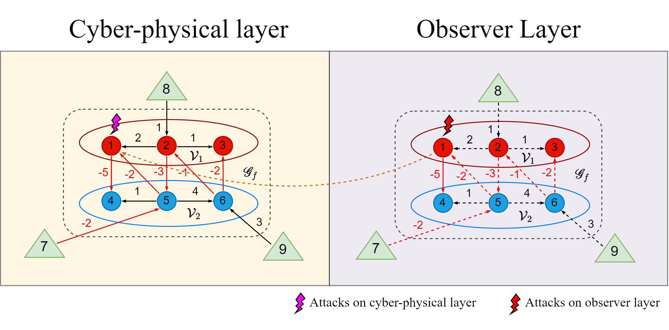
Figure 1: Cyber-physical layer and observer layer.

In this section, we develop fully-distributed attack-resilient control strategies to solve the ARBOC problem for heterogeneous MASs by using a bi-layer defense architecture. We first construct dynamic compensators communicating on the OL (Fig. 1) to estimate the convex combinations of the sates and negative states of the leaders. While prevailing literature generally assumes that there is no cyber-attack on the OL, we relax such strict limitation by considering the potential cyber-attacks on the OL. The information flow among agents are represented by arrows, with the corresponding edge weight values annotated adjacent to them. Positive edge weight values indicate cooperative relationships and negative edge weight values indicate antagonistic relationships. We consider a more practical and challenging scenario where the OL is also subjected to cyber-attacks, necessitating the design of an attack-resilient dynamic compensators.

For convenience, we first define the following neighborhood bipartite state containment information on the OL

$$\xi_{i}=\sum_{j\in\mathscr{F}}(a_{ij}\zeta_{j}-|a_{ij}|\zeta_{i})+\sum_{r\in\mathscr{L}}(g_{ir}x_{r}-|g_{ir}|\zeta_{i}),$$ (15)

where $\zeta_{i}$ is the local state of the dynamic compensator. Then, we develop the following fully-distributed attack-resilient compensator against EU-FDI attacks on the OL

$${{\dot{\zeta}}_{i}}=S{\zeta_{i}}+\exp{(\vartheta_{i})}{\xi_{i}}+\gamma^{OL}_{i},$$ (16)

$${{\dot{\vartheta}}_{i}}=q_{i}\xi_{i}^{T}{\xi_{i}},$$ (17)

where ${\vartheta_{i}}$ is an adaptive coupling gain tuned by (17) with ${\vartheta_{i}}\left(0\right)\geqslant 0$, $\gamma^{OL}_{i}$ denotes the EU-FDI attack signal targeting compensator $i$ on the OL, and $q_{i}>0$ is the adaptive tuning gain.

Remark 2.

Observer design is generally employed to estimate the states of the leaders for heterogeneous MASs. However, most of the literature assumes that the observers remain intact against cyber-attacks, which is not practical. In contrast, we consider more general and practical scenarios in which the observers could also be attacked.

Remark 3.

In [25], the knowledge of the global graph topology is required in the scalar coupling design. However, as seen from Eq. (17), no knowledge of the global graph topology is required in the design of the adaptive coupling gain $\vartheta_{i}$. Hence, the controller is fully-distributed.

Definition 5.

A signal $\gamma(t)\in{\mathbb{R}^{n}}$ is said to be exponentially unbounded if its norm grows at most exponentially with time, i.e., there exists a positive constant $\kappa$, such that $\|\gamma(t)\|\leqslant\exp(\kappa t)$, where $\kappa$ could be unknown.

Assumption 6.

$\gamma^{a}_{i}(t)$ and $\gamma^{OL}_{i}(t)$ are exponentially unbounded signals, i.e., there exist positive constants $\kappa^{a}_{i}$ and $\kappa^{OL}_{i}$, such that $\|\gamma^{a}_{i}(t)\|\leqslant\exp(\kappa^{a}_{i}t)$ and $\|\gamma^{OL}_{i}(t)\|\leqslant\exp(\kappa^{OL}_{i}t)$.

Remark 4.

Assumption 6 describes a wide range of FDI attack signals, including those that grow exponentially over time. Note that $\exp(\kappa^{a}_{i}t)$ and $\exp(\kappa^{OL}_{i}t)$ are the worst-case scenario the controller can manage, i.e., as long as the growth rate of the attack signal over time is less than $\exp(\kappa^{a}_{i}t)$ and $\exp(\kappa^{OL}_{i}t)$, they can be mitigated. Therefore, the controller is capable of handling a wide range of FDI attack signals. In reality, adversaries can inject any time-varying signal into systems via software, CPU, DSP, or similar platforms. However, existing literature only deals with noises, disturbances or bounded attack signals, or it is required that the first-order time derivatives of the attacks be bounded [20]. The primary threat of these signals lies in their ability to cause system instability, as their rapid growth can quickly lead to significant disruptions. This necessitates comprehensive and strategic defense mechanisms to ensure the stability and security of MASs against these EU-FDI attacks.

Define the following state tracking error

$${\varepsilon_{i}}={x_{i}}-{\Pi_{i}}{\zeta_{i}}.$$ (18)

Building on the dynamic resilient compensator design, we finally introduce the following fully-distributed attack-resilient controller design.

$${u_{i}}={K_{i}}{x_{i}}+{H_{i}}{\zeta_{i}}-\hat{\gamma}^{a}_{i},$$ (19)

$${\hat{\gamma}^{a}_{i}}=\frac{{B_{i}^{T}{P_{i}}{\varepsilon_{i}}}}{{\left\|{{\varepsilon_{i}}^{T}{P_{i}}{B_{i}}}\right\|+\exp\left(-c_{i}t^{2}\right)}}\exp(\hat{\rho}_{i}),$$ (20)

$${{\dot{\hat{\rho}}}_{i}}={\alpha_{i}\left\|{{\varepsilon_{i}}^{T}{P_{i}}{B_{i}}}\right\|},$$ (21)

where $\hat{\gamma}^{a}_{i}$ is a compensational signal designed per (20) to mitigate the adverse effect caused by the actuator attack signal $\gamma^{a}_{i}$, $\hat{\rho}_{i}$ is an adaptive coupling gain tuned by (21), $\alpha_{i}$ and $c_{i}$ are positive constants. Employ certain positive-definite symmetric matrices $U_{i}$ and $Q_{i}$, under Assumption 4, the solution $P_{i}$ to the following algebraic Riccati equation can be found.

$$A_{i}^{T}P_{i}+P_{i}A_{i}+Q_{i}-P_{i}B_{i}{U_{i}^{-1}}{B_{i}^{T}}{P_{i}}=0.$$ (22)

The controller gain matrices $K_{i}$ and $H_{i}$ in (19) are designed as

$${K_{i}}=-U_{i}^{-1}B_{i}^{T}{P_{i}},$$ (23)

$$H_{i}=\Gamma_{i}-K_{i}{\Pi_{i}},$$ (24)

Next, we present the main result for solving the ARBOC problem for heterogeneous MASs.

Theorem 1.

Given Assumptions 1 to 6, considering the heterogeneous MAS composed of (1) and (3) in the presence of EU-FDI attacks on both CPL and OL, Problem 1 is solved by designing the fully-distributed controller consisting of (15) to (24).

Proof: From Lemma 4, to prove that Problem 1 is solved, we need to prove that $e^{s}_{y}$ is UUB. Note that $e^{s}_{y}$ in (9) can be written as

$$\begin{gathered}e^{s}_{y}=-\sum_{\nu\in\mathscr{L}}(\Phi_{\nu}^{s}\otimes I_{z})\Bigg{(}y-\hfill\\ \sum_{r\in\mathscr{L}}\left(\left(\sum_{k\in\mathscr{L}}\Phi_{k}^{s}\right)^{-1}\otimes I_{z}\right)\left(\left(\frac{1}{M}\bar{\mathcal{L}}+\mathcal{G}_{r}\right)\otimes I_{z}\right)\bar{y}_{r}\Bigg{)}\\ =-\sum_{\nu\in\mathscr{L}}(\Phi_{\nu}^{s}\otimes I_{z})\Bigg{(}\operatorname{diag}(C_{i})x-\hfill\\ \sum_{r\in\mathscr{L}}\left(\left(\sum_{k\in\mathscr{L}}\Phi_{k}^{s}\right)^{-1}\otimes I_{z}\right)\left(\left(\frac{1}{M}\bar{\mathcal{L}}+\mathcal{G}_{r}\right)\otimes I_{z}\right)\hfill\\ \times(I_{N}\otimes R)\bar{x}_{r}\Bigg{)}\hfill\\ =-\sum_{\nu\in\mathscr{L}}(\Phi_{\nu}^{s}\otimes I_{z})\Bigg{(}\operatorname{diag}(C_{i})x-(I_{N}\otimes R)\times\hfill\\ \sum_{r\in\mathscr{L}}\Bigg{(}\left(\sum_{k\in\mathscr{L}}\Phi_{k}^{s}\right)^{-1}\left(\frac{1}{M}\bar{\mathcal{L}}+\mathcal{G}_{r}\right)\otimes I_{l}\Bigg{)}\bar{x}_{r}\Bigg{)}\hfill\\ =-\sum_{\nu\in\mathscr{L}}(\Phi_{\nu}^{s}\otimes I_{z})\Bigg{(}\operatorname{diag}(C_{i})x-\operatorname{diag}(C_{i}\Pi_{i})\hfill\\ \times\sum_{r\in\mathscr{L}}\Bigg{(}\left(\sum_{k\in\mathscr{L}}\Phi_{k}^{s}\right)^{-1}\left(\frac{1}{M}\bar{\mathcal{L}}+\mathcal{G}_{r}\right)\otimes I_{l}\Bigg{)}\bar{x}_{r}\Bigg{)}\hfill\\ =-\sum_{\nu\in\mathscr{L}}(\Phi_{\nu}^{s}\otimes I_{z})\operatorname{diag}(C_{i})\Bigg{(}\varepsilon+\operatorname{diag}(\Pi_{i})\hfill\\ \times\Bigg{(}\zeta-\sum_{r\in\mathscr{L}}\Bigg{(}\left(\sum_{k\in\mathscr{L}}\Phi_{k}^{s}\right)^{-1}\left(\frac{1}{M}\bar{\mathcal{L}}+\mathcal{G}_{r}\right)\otimes I_{l}\Bigg{)}\hfill\\ \times\bar{x}_{r}\Bigg{)}\Bigg{)}\Bigg{)},\hfill\end{gathered}$$ (25)

where $\varepsilon={[{\varepsilon_{1}^{T},...,\varepsilon_{N}^{T}}]^{T}}$, $\zeta={[{\zeta_{1}^{T},...,\zeta_{N}^{T}}]^{T}}$ and $\bar{x}_{r}={[{x_{N+1}^{T},...,x_{N+M}^{T}}]^{T}}$. Define the following global compensator containment error

$$\begin{gathered}\delta=\zeta-\sum_{r\in\mathscr{L}}\Bigg{(}\left(\sum_{k\in\mathscr{L}}\Phi_{k}^{s}\right)^{-1}\left(\frac{1}{M}\bar{\mathcal{L}}+\mathcal{G}_{r}\right)\otimes I_{l}\Bigg{)}\bar{x}_{r}.\end{gathered}$$ (26)

Then, we obtain

$$e^{s}_{y}=-\sum_{\nu\in\mathscr{L}}(\Phi_{\nu}^{s}\otimes I_{z})\operatorname{diag}(C_{i})\big{(}\varepsilon+\operatorname{diag}(\Pi_{i})\delta\big{)}.\hfill$$ (27)

To show that $e^{s}_{y}$ is UUB, we will prove that $\varepsilon$ and $\delta$ are UUB in the following analysis.

Note that the global form of (15) is

$$\begin{gathered}\xi=-\sum_{\nu\in\mathscr{L}}(\Phi_{\nu}^{s}\otimes I_{l})\Bigg{(}\zeta-\hfill\\ \sum_{r\in\mathscr{L}}\left(\left(\sum_{k\in\mathscr{L}}\Phi_{k}^{s}\right)^{-1}\otimes I_{l}\right)\left(\left(\frac{1}{M}\bar{\mathcal{L}}+\mathcal{G}_{r}\right)\otimes I_{l}\right)\bar{x}_{r}\Bigg{)}\hfill\\ =-\sum_{\nu\in\mathscr{L}}(\Phi_{\nu}^{s}\otimes I_{l})\Bigg{(}\zeta-\hfill\\ \sum_{r\in\mathscr{L}}\Bigg{(}\left(\sum_{k\in\mathscr{L}}\Phi_{k}^{s}\right)^{-1}\left(\frac{1}{M}\bar{\mathcal{L}}+\mathcal{G}_{r}\right)\otimes I_{l}\Bigg{)}\bar{x}_{r}\Bigg{)}\hfill\\ =-\sum_{\nu\in\mathscr{L}}(\Phi_{\nu}^{s}\otimes I_{l})\delta,\hfill\end{gathered}$$ (28)

where $\xi={[{\xi_{1}^{T},...,\xi_{N}^{T}}]^{T}}$. Since $\sum_{\nu\in\mathscr{L}}(\Phi_{\nu}^{s}\otimes I_{l})$ is nonsingular based on Lemma 2, to prove that $\delta$ is UUB is equivalent to proving that $\xi$ is UUB.

The global form of $\dot{\zeta}_{i}$ in (16) is

$$\begin{gathered}\dot{\zeta}=(I_{N}\otimes S)\zeta+\operatorname{diag}(\exp(\vartheta_{i}))\xi+\gamma^{OL}.\hfill\end{gathered}$$ (29)

where $\gamma^{OL}={[{{\gamma^{OL}_{1}}^{T},...,{\gamma^{OL}_{N}}^{T}}]^{T}}$. Then the time derivative of $\xi$ in (28) is

$$\begin{gathered}\dot{\xi}=-\sum_{\nu\in\mathscr{L}}(\Phi_{\nu}^{s}\otimes I_{l})\Bigg{(}\dot{\zeta}-\hfill\\ \sum_{r\in\mathscr{L}}\Bigg{(}\left(\sum_{k\in\mathscr{L}}\Phi_{k}^{s}\right)^{-1}\left(\frac{1}{M}\bar{\mathcal{L}}+\mathcal{G}_{r}\right)\otimes I_{l}\Bigg{)}\dot{\bar{x}}_{r}\Bigg{)}\hfill\\ =-\sum_{\nu\in\mathscr{L}}(\Phi_{\nu}^{s}\otimes I_{l})\Bigg{(}(I_{N}\otimes S)\zeta+\big{(}\operatorname{diag}(\exp(\vartheta_{i}))\otimes{I_{l}}\big{)}\xi\hfill\\ +\gamma^{OL}-\sum_{r\in\mathscr{L}}\Bigg{(}\left(\sum_{k\in\mathscr{L}}\Phi_{k}^{s}\right)^{-1}\left(\frac{1}{M}\bar{\mathcal{L}}+\mathcal{G}_{r}\right)\otimes I_{l}\Bigg{)}\hfill\\ \times(I_{N}\otimes S)\bar{x}_{r}\Bigg{)}\hfill\\ =(I_{N}\otimes S)\xi-\sum_{r\in\mathscr{L}}(\Phi_{r}^{s}\otimes I_{l})\big{(}\operatorname{diag}(\exp(\vartheta_{i}))\otimes{I_{l}}\big{)}\xi\hfill\\ -\sum_{r\in\mathscr{L}}(\Phi_{r}^{s}\otimes I_{l})\gamma^{OL}.\hfill\end{gathered}$$ (30)

We consider the following Lyapunov function candidate

$$V^{{}^{\prime}}=\frac{1}{2}\sum\limits_{i=1}^{N}\xi_{i}^{T}\xi_{i}\exp(\vartheta_{i}).$$ (31)

The time derivative of $V^{{}^{\prime}}$ along the trajectory of (30) is given by

$$\begin{gathered}\dot{V}^{{}^{\prime}}=\sum\limits_{i=1}^{N}\big{(}\xi_{i}^{T}{\dot{\xi}_{i}}\exp(\vartheta_{i})+\frac{1}{2}\xi^{T}_{i}\xi_{i}\exp(\vartheta_{i})\dot{\vartheta}_{i}\big{)}\hfill\\ =\xi^{T}\operatorname{diag}\big{(}\exp(\vartheta_{i})\otimes I_{l}\big{)}\dot{\xi}+\frac{1}{2}\xi^{T}_{i}\big{(}\operatorname{diag}(\exp(\vartheta_{i})\dot{\vartheta}_{i})\otimes I_{l}\big{)}\hfill\\ \times\xi\hfill\\ =\xi^{T}\operatorname{diag}\big{(}\exp(\vartheta_{i})\otimes I_{l}\big{)}\bigg{(}(I_{N}\otimes S)\xi-\sum_{r\in\mathscr{L}}(\Phi_{r}^{s}\otimes I_{l})\hfill\\ \times\big{(}\operatorname{diag}(\exp(\vartheta_{i}))\otimes{I_{l}}\big{)}\xi-\sum_{r\in\mathscr{L}}(\Phi_{r}^{s}\otimes I_{l})\gamma^{OL}\bigg{)}+\frac{1}{2}\xi^{T}\hfill\\ \times\big{(}\operatorname{diag}(\dot{\vartheta}_{i})\otimes I_{l}\big{)}\big{(}\operatorname{diag}(\exp(\vartheta_{i}))\otimes I_{l}\big{)}\xi\hfill\\ \leqslant\sigma_{\max}(S)\|\big{(}\operatorname{diag}(\exp(\vartheta_{i}))\otimes{I_{l}}\big{)}\xi\|\|\xi\|-\sigma_{\min}\big{(}\sum_{r\in\mathscr{L}}\Phi_{r}^{s}\big{)}\hfill\\ \times\|\big{(}\operatorname{diag}(\exp(\vartheta_{i}))\otimes{I_{l}}\big{)}\xi\|^{2}+\sigma_{\max}\big{(}\sum_{r\in\mathscr{L}}\Phi_{r}^{s}\big{)}\hfill\\ \times\|\big{(}\operatorname{diag}(\exp(\vartheta_{i}))\otimes{I_{l}}\big{)}\xi\|\|\gamma^{OL}\|+\frac{1}{2}\max_{i}(\dot{\vartheta}_{i})\hfill\\ \times\|\big{(}\operatorname{diag}(\exp(\vartheta_{i}))\otimes{I_{l}}\big{)}\xi\|\|\xi\|\hfill\\ =-\sigma_{\min}\big{(}\sum_{r\in\mathscr{L}}\Phi_{r}^{s}\big{)}\|\big{(}\operatorname{diag}(\exp(\vartheta_{i}))\otimes{I_{l}}\big{)}\xi\|\hfill\\ \times\bigg{(}\|\big{(}\operatorname{diag}(\exp(\vartheta_{i}))\otimes{I_{l}}\big{)}\xi\|-\sigma_{\max}(S)\hfill\\ /\sigma_{\min}\big{(}\sum_{r\in\mathscr{L}}\Phi_{r}^{s}\big{)}\|\xi\|-\sigma_{\max}\big{(}\sum_{r\in\mathscr{L}}\Phi_{r}^{s}\big{)}/\sigma_{\min}\big{(}\sum_{r\in\mathscr{L}}\Phi_{r}^{s}\big{)}\hfill\\ \times\|\gamma^{OL}\|-\frac{1}{2}\max_{i}(\dot{\vartheta}_{i})/\sigma_{\min}\big{(}\sum_{r\in\mathscr{L}}\Phi_{r}^{s}\big{)}\|\xi\|\bigg{)}.\hfill\\ \end{gathered}$$ (32)

For convenience, denote $\phi_{a}=\sigma_{\max}(S)/\sigma_{\min}\big{(}\sum_{r\in\mathscr{L}}\Phi_{r}^{s}\big{)}$ and $\phi_{b}=\sigma_{\max}\big{(}\sum_{r\in\mathscr{L}}\Phi_{r}^{s}\big{)}/\sigma_{\min}\big{(}\sum_{r\in\mathscr{L}}\Phi_{r}^{s}\big{)}$, which are both positive constants. To let $\dot{V}^{{}^{\prime}}\leqslant 0$, we need

$$\begin{gathered}\|\big{(}\operatorname{diag}(\exp(\vartheta_{i}))\otimes{I_{l}}\big{)}\xi\|-\phi_{a}\|\xi\|-\phi_{b}\|\gamma^{OL}\|\hfill\\ -\frac{1}{2}\max_{i}(\dot{\vartheta}_{i})/\sigma_{\min}\big{(}\sum_{r\in\mathscr{L}}\Phi_{r}^{s}\big{)}\|\xi\|\geqslant 0.\hfill\end{gathered}$$ (33)

A sufficient condition to guarantee (33) is

$$\begin{gathered}\big{(}\exp(\vartheta_{i})-\phi_{a}-\frac{1}{2}\max_{i}(\dot{\vartheta}_{i})/\sigma_{\min}\big{(}\sum_{r\in\mathscr{L}}\Phi_{r}^{s}\big{)}\big{)}\|\xi_{i}\|\hfill\\ \geqslant\phi_{b}\|\gamma^{OL}_{i}\|.\hfill\end{gathered}$$ (34)

A sufficient condition to guarantee (34) is $\|\xi_{i}\|\geqslant\phi_{b}$ and $\exp(\vartheta_{i})-\phi_{a}-1/2\max_{i}(\dot{\vartheta}_{i})/\sigma_{\min}(\sum_{r\in\mathscr{L}}\Phi_{r}^{s})\geqslant\|\gamma^{OL}_{i}\|$. From Assumption 6, $\|\gamma^{OL}_{i}(t)\|\leqslant\exp(\kappa^{OL}_{i}t)$, to prove that $\exp(\vartheta_{i})-\phi_{a}-1/2\max_{i}(\dot{\vartheta}_{i})/\sigma_{\min}(\sum_{r\in\mathscr{L}}\Phi_{r}^{s})\geqslant\|\gamma^{OL}_{i}\|$, we need to prove that $\exp(\vartheta_{i})-\phi_{a}-1/2\max_{i}(\dot{\vartheta}_{i})/\sigma_{\min}(\sum_{r\in\mathscr{L}}\Phi_{r}^{s})\geqslant\exp(\kappa^{OL}_{i}t)$. Based on (17), when $\|\xi_{i}\|>\max\{\sqrt{\kappa^{OL}_{i}/q_{i}},\phi_{b}\}$, which guarantees the exponential growth of $\exp(\vartheta_{i})$ dominates all other terms, $\exists t_{1}$ such that $\forall t>t_{1}$, $\exp(\vartheta_{i})-\phi_{a}-1/2\max_{i}(\dot{\vartheta}_{i})/\sigma_{\min}(\sum_{r\in\mathscr{L}}\Phi_{r}^{s})\geqslant\exp(\kappa^{OL}_{i}t)$. Hence, we obtain $\forall t>t_{1}$,

$$\dot{V}^{{}^{\prime}}\leqslant 0,\>\forall\|\xi_{i}\|>\max\{\sqrt{\kappa^{OL}_{i}/q_{i}},\phi_{b}\}.$$ (35)

By LaSalle’s invariance principle [28], $\xi_{i}$ is UUB.

Next, we prove that $\varepsilon$ is UUB. From (1), (6), (16), (19) and (24), we obtain the time derivative of (18) as

$$\begin{gathered}{{\dot{\varepsilon}}_{i}}={{\dot{x}}_{i}}-{\Pi_{i}}{{\dot{\zeta}}_{i}}\hfill\\ ={A_{i}}{x_{i}}+{B_{i}}{K_{i}}{x_{i}}+{B_{i}}{H_{i}}{\zeta_{i}}-{B_{i}}{\hat{\gamma}^{a}_{i}}\hfill\\ +{B_{i}}{\gamma^{a}_{i}}-{\Pi_{i}}S{\zeta_{i}}-{\Pi_{i}}\exp(\vartheta_{i}){\xi_{i}}-\Pi_{i}\gamma^{OL}_{i}\hfill\\ =\left({{A_{i}}+{B_{i}}{K_{i}}}\right){\varepsilon_{i}}+{B_{i}}{\gamma^{a}_{i}}-{B_{i}}{\hat{\gamma}^{a}_{i}}-{\Pi_{i}}\exp(\vartheta_{i}){\xi_{i}}-\Pi_{i}\gamma^{OL}_{i}.\hfill\end{gathered}$$ (36)

From the above proof, we confirmed ${\xi_{i}}$ is UUB. Considering Assumption 2, (28) and (29), we obtain that $\beta_{i}\equiv{\Pi_{i}}\exp(\vartheta_{i}){\xi_{i}}+\Pi_{i}\gamma^{OL}_{i}$ is bounded. Let ${{\bar{A}}_{i}}={A_{i}}+{B_{i}}{K_{i}}$ and ${\bar{Q}_{i}}={Q_{i}}+K_{i}^{T}{U_{i}}{K_{i}}$. Note that ${\bar{Q}_{i}}$ is positive-definite. From (22), $P_{i}$ is symmetric positive-definite. Consider the following Lyapunov function candidate

$$V_{i}=\varepsilon_{i}^{T}P_{i}\varepsilon_{i},$$ (37)

and its time derivative is given by

$$\begin{gathered}\dot{V}_{i}=2\varepsilon^{T}_{i}P_{i}\dot{\varepsilon}_{i}\hfill\\ =2\varepsilon_{i}^{T}P_{i}\left(\bar{A}_{i}\varepsilon_{i}+B_{i}\gamma^{a}_{i}-B_{i}\hat{\gamma}^{a}_{i}-\beta_{i}\right)\hfill\\ \leqslant-\sigma_{\min}\left(\bar{Q}_{i}\right)\left\|\varepsilon_{i}\right\|^{2}+2\left(\varepsilon_{i}^{T}P_{i}B_{i}\gamma^{a}_{i}-\varepsilon_{i}^{T}P_{i}B_{i}\hat{\gamma}^{a}_{i}\right)\hfill\\ -2\varepsilon_{i}^{T}P_{i}\beta_{i}\hfill\\ \leqslant-\sigma_{\min}\left(\bar{Q}_{i}\right)\left\|\varepsilon_{i}\right\|^{2}+2\left(\varepsilon_{i}^{T}P_{i}B_{i}\gamma^{a}_{i}-\varepsilon_{i}^{T}P_{i}B_{i}\hat{\gamma}^{a}_{i}\right)\hfill\\ +2\sigma_{\max}\left(P_{i}\right)\left\|\varepsilon_{i}\right\|\left\|\beta_{i}\right\|.\hfill\\ \end{gathered}$$ (38)

Using (20) to obtain

$$\begin{gathered}\varepsilon_{i}^{T}P_{i}B_{i}\gamma^{a}_{i}-\varepsilon_{i}^{T}P_{i}B_{i}\hat{\gamma}^{a}_{i}\hfill\\ =\varepsilon_{i}^{T}P_{i}B_{i}\gamma^{a}_{i}-\frac{\left\|\varepsilon_{i}^{T}P_{i}B_{i}\right\|^{2}}{\left\|\varepsilon_{i}^{T}P_{i}B_{i}\right\|+\exp\left(-c_{i}t^{2}\right)}\exp\left(\hat{\rho}_{i}\right)\hfill\\ \leqslant\left\|\varepsilon_{i}^{T}P_{i}B_{i}\right\|\left\|\gamma^{a}_{i}\right\|-\frac{\left\|\varepsilon_{i}^{T}P_{i}B_{i}\right\|^{2}}{\left\|\varepsilon_{i}^{T}P_{i}B_{i}\right\|+\exp\left(-c_{i}t^{2}\right)}\exp\left(\hat{\rho}_{i}\right)\hfill\\ =\left\|\varepsilon_{i}^{T}P_{i}B_{i}\right\|\big{(}\left\|\varepsilon_{i}^{T}P_{i}B_{i}\right\|\left\|\gamma^{a}_{i}\right\|+\exp(-c_{i}t^{2})\left\|\gamma^{a}_{i}\right\|\hfill\\ -\left\|\varepsilon_{i}^{T}P_{i}B_{i}\right\|\exp\left(\hat{\rho}_{i}\right)\big{)}/\big{(}\left\|\varepsilon_{i}^{T}P_{i}B_{i}\right\|+\exp(-c_{i}t^{2})\big{)}.\hfill\end{gathered}$$ (39)

To prove that $\varepsilon_{i}^{T}P_{i}B_{i}\gamma^{a}_{i}-\varepsilon_{i}^{T}P_{i}B_{i}\hat{\gamma}^{a}_{i}\leqslant 0$, we need to prove that $\left\|\varepsilon_{i}^{T}P_{i}B_{i}\right\|\left\|\gamma^{a}_{i}\right\|+\exp(-c_{i}t^{2})\left\|\gamma^{a}_{i}\right\|-\left\|\varepsilon_{i}^{T}P_{i}B_{i}\right\|\exp\left(\hat{\rho}_{i}\right)\leqslant 0$. Define $\upsilon_{i}=\kappa^{a}_{i}/\sigma_{\operatorname{min}}(P_{i}B_{i})$, $\omega_{i}=2\sigma_{\max}\left(P_{i}\right)\left\|\beta_{i}\right\|/\sigma_{\min}\left(\bar{Q}_{i}\right)$. Then, define the compact sets $\Upsilon_{i}\equiv\ \{\|\varepsilon_{i}\|\leqslant\upsilon_{i}\}$ and $\Omega_{i}\equiv\{\|\varepsilon_{i}\|\leqslant\omega_{i}\}$. Considering Assumption 6, we obtain that $\exp(-c_{i}t^{2})\left\|\gamma^{a}_{i}\right\|\rightarrow 0$. Hence, outside the compact set $\Upsilon_{i}\equiv\ \{\|\varepsilon_{i}\|\leqslant\upsilon_{i}\}$, $\exists t_{1}$, such that $\varepsilon_{i}^{T}P_{i}B_{i}\gamma^{a}_{i}-\varepsilon_{i}^{T}P_{i}B_{i}\hat{\gamma}^{a}_{i}\leqslant 0$, $\forall t\geqslant t_{1}$; outside the compact set $\Omega_{i}\equiv\{\|\varepsilon_{i}\|\leqslant\omega_{i}\}$, $-\sigma_{\min}\left(\bar{Q}_{i}\right)\left\|\varepsilon_{i}\right\|^{2}+2\sigma_{\max}\left(P_{i}\right)\left\|\varepsilon_{i}\right\|\left\|\beta_{i}\right\|\leqslant 0$. Therefore, combining (38), (39) and (36), we obtain, outside the compact set $\Upsilon_{i}\cup\Omega_{i}$, $\forall t\geqslant t_{1}$,

$$\dot{V}_{i}\leqslant 0.$$ (40)

Hence, by the LaSalle’s invariance principle, $\varepsilon_{i}$ is UUB. Consequently, we conclude that $e^{s}_{y}$ is UUB. This completes the proof. $\hfill\blacksquare$

IV Numerical Simulations

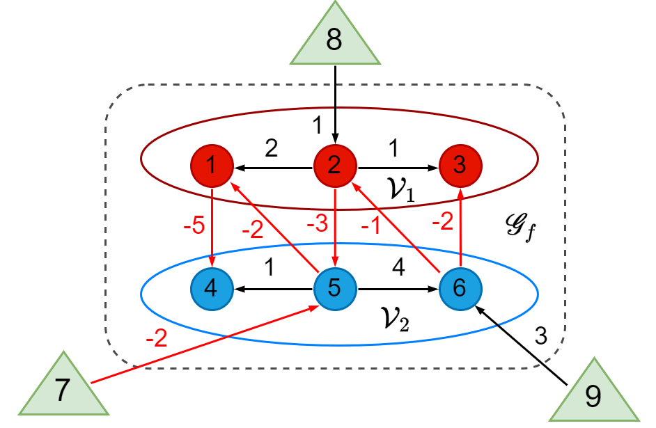
Figure 2: Communication topology.

In this section, we validate our proposed cyber-physical defense strategies within a general heterogeneous MAS, specifically verifying the effectiveness and resilience of the control protocols against EU-FDI attack signals. The communication topology of the heterogeneous MAS is delineated in Fig. 2. The system comprises six followers represented by circles and three leaders represented by triangles. The dynamics of the followers and leaders are given by:

$$\begin{gathered}\left\{\begin{gathered}\dot{x}_{1,2}=\left[\begin{array}[]{*{2}{c}}-2&1\\ 0&-3\end{array}\right]x_{1,2}+\left[\begin{array}[]{*{2}{c}}1&0\\ 0&1\end{array}\right]u_{1,2}\hfill\\ y_{1,2}=\left[\begin{array}[]{*{2}{c}}0.5&1\\ 1&0.5\end{array}\right]x_{1,2}\hfill\\ \end{gathered}\right.\hfill\\ \left\{\begin{gathered}\dot{x}_{3,4}=\left[\begin{array}[]{*{2}{c}}-1&0\\ 0&-2\end{array}\right]x_{3,4}+\left[\begin{array}[]{*{2}{c}}0.5&1\\ 1&0.5\end{array}\right]u_{3,4}\hfill\\ y_{3,4}=\left[\begin{array}[]{*{2}{c}}1&0.5\\ 0.5&1\end{array}\right]x_{3,4}\hfill\\ \end{gathered}\right.\hfill\\ \left\{\begin{gathered}\dot{x}_{5,6}=\left[\begin{array}[]{*{3}{c}}-1&0&0\\ 0&-2&0\\ 0&0&-3\end{array}\right]x_{5,6}+\left[\begin{array}[]{*{2}{c}}1&0\\ 0&1\\ 1&0\end{array}\right]u_{5,6}\hfill\\ y_{5,6}=\left[\begin{array}[]{*{3}{c}}1&0&-1\\ 0&1&1\end{array}\right]x_{5,6}\hfill\\ \end{gathered}\right.\hfill\\ \left\{\begin{gathered}\dot{x}_{7,8,9}=\left[\begin{array}[]{*{2}{c}}0&-2\\ 1&0\end{array}\right]x_{7,8,9},\\ y_{7,8,9}=\left[\begin{array}[]{*{2}{c}}1&0\\ 0&1\end{array}\right]x_{7,8,9}\hfill\\ \end{gathered}\right.\hfill\\ \end{gathered}\\$$

We choose the following EU-FDI attack signals injected on CPL and OL:

$$\gamma^{a}_{1} =\begin{bmatrix}20e^{0.2t}\\ 20e^{0.2t}\end{bmatrix}, \gamma^{OL}_{1} =\begin{bmatrix}-20e^{0.2t}\\ -20e^{0.2t}\end{bmatrix},$$

$$\gamma^{a}_{2} =\begin{bmatrix}20e^{0.2t}\\ -20e^{0.2t}\end{bmatrix}, \gamma^{OL}_{2} =\begin{bmatrix}20e^{0.2t}\\ 20e^{0.2t}\end{bmatrix},$$

$$\gamma^{a}_{3} =\begin{bmatrix}20e^{0.2t}\\ -20e^{0.2t}\end{bmatrix}, \gamma^{OL}_{3} =\begin{bmatrix}-20e^{0.2t}\\ -20e^{0.2t}\end{bmatrix},$$

$$\gamma^{a}_{4} =\begin{bmatrix}20e^{0.2t}\\ -20e^{0.2t}\end{bmatrix}, \gamma^{OL}_{4} =\begin{bmatrix}20e^{0.2t}\\ 20e^{0.2t}\end{bmatrix},$$

$$\gamma^{a}_{5} =\begin{bmatrix}20e^{0.2t}\\ 20e^{0.2t}\end{bmatrix}, \gamma^{OL}_{5} =\begin{bmatrix}-20e^{0.2t}\\ -20e^{0.2t}\end{bmatrix},$$

$$\gamma^{a}_{6} =\begin{bmatrix}-20e^{0.2t}\\ 20e^{0.2t}\end{bmatrix}, \gamma^{OL}_{6} =\begin{bmatrix}20e^{0.2t}\\ 20e^{0.2t}\end{bmatrix}.$$

These exponentially growing attack signals are designed to test the system’s resilience and adaptability in dynamic adversarial scenarios. The following pairs $(\Pi_{i},\Gamma_{i})$ are obtained for each follower by solving (6)

$$\begin{gathered}{\Pi_{1,2}}=\left[{\begin{array}[]{*{20}{c}}{-0.67}&{1.33}\\ {1.33}&{-0.67}\end{array}}\right],{\Gamma_{1,2}}=\left[{\begin{array}[]{*{20}{c}}{-1.33}&{4.67}\\ {3.33}&{-4.67}\end{array}}\right],\hfill\\ {\Pi_{3,4}}=\left[{\begin{array}[]{*{20}{c}}{1.33}&{-0.67}\\ {-0.67}&{1.33}\end{array}}\right],{\Gamma_{3,4}}=\left[{\begin{array}[]{*{20}{c}}{-0.44}&{7.56}\\ {0.89}&{-7.11}\end{array}}\right],\hfill\\ {\Pi_{5,6}}=\left[{\begin{array}[]{*{20}{c}}{1.50}&{-1.00}\\ {-0.50}&{2.00}\\ {0.50}&{-1.00}\end{array}}\right],{\Gamma_{5,6}}=\left[{\begin{array}[]{*{20}{c}}{0.50}&{-4.00}\\ {1.00}&{5.00}\end{array}}\right].\hfill\\ \end{gathered}\\$$

Select $U_{1,2,...,6}=I_{2}$, $Q_{1,2,3,4}=3I_{2}$, and $Q_{5,6}=3I_{3}$. The controller gain matrices $K_{i}$ and $H_{i}$ found by solving (23) to (22) are

$$\begin{gathered}{K_{1,2}}=\left[{\begin{array}[]{*{20}{c}}{-0.64}&{-0.10}\\ {-0.10}&{-0.49}\end{array}}\right],{H_{1,2}}=\left[{\begin{array}[]{*{20}{c}}{-1.62}&{5.46}\\ {3.92}&{-4.86}\end{array}}\right],\hfill\\ {K_{3,4}}=\left[{\begin{array}[]{*{20}{c}}{-0.37}&{-0.59}\\ {-0.93}&{-0.19}\end{array}}\right],{H_{3,4}}=\left[{\begin{array}[]{*{20}{c}}{-0.35}&{8.09}\\ {2.00}&{-7.47}\end{array}}\right],\hfill\\ {K_{5,6}}=\left[{\begin{array}[]{*{20}{c}}{-0.95}&{0}&{-0.38}\\ {0}&{-0.65}&{0}\end{array}}\right],\hfill\\ {H_{5,6}}=\left[{\begin{array}[]{*{20}{c}}{2.12}&{-5.34}\\ {0.68}&{6.29}\end{array}}\right].\hfill\\ \end{gathered}\\$$

For comparison, we run the simulation using the standard bipartite output containment control protocols as follows.

$$\begin{gathered}\left\{\begin{gathered}{{\dot{\zeta}}_{i}}=S{\zeta_{i}}+\vartheta_{i}{\xi_{i}},\hfill\\ {{\dot{\vartheta}}_{i}}=q_{i}\xi_{i}^{T}{\xi_{i}},\hfill\\ {u_{i}}={K_{i}}{x_{i}}+{H_{i}}{\zeta_{i}}.\hfill\end{gathered}\right.\end{gathered}$$ (41)

Next, we evaluate the system’s resilience against EU-FDI attacks on CPL and OL using the standard bipartite output containment control protocols and the proposed cyber-physical defense strategies. The outputs and the negative outputs of the leaders and the outputs of the followers are captured as snapshots at three time instants in both comparative simulation case studies, where the outputs of leaders are denoted by green triangles, and the negative outputs of leaders are denoted by purple triangles. The EU-FDI attacks on CPL and OL are initiated simultaneously at $8$ s.

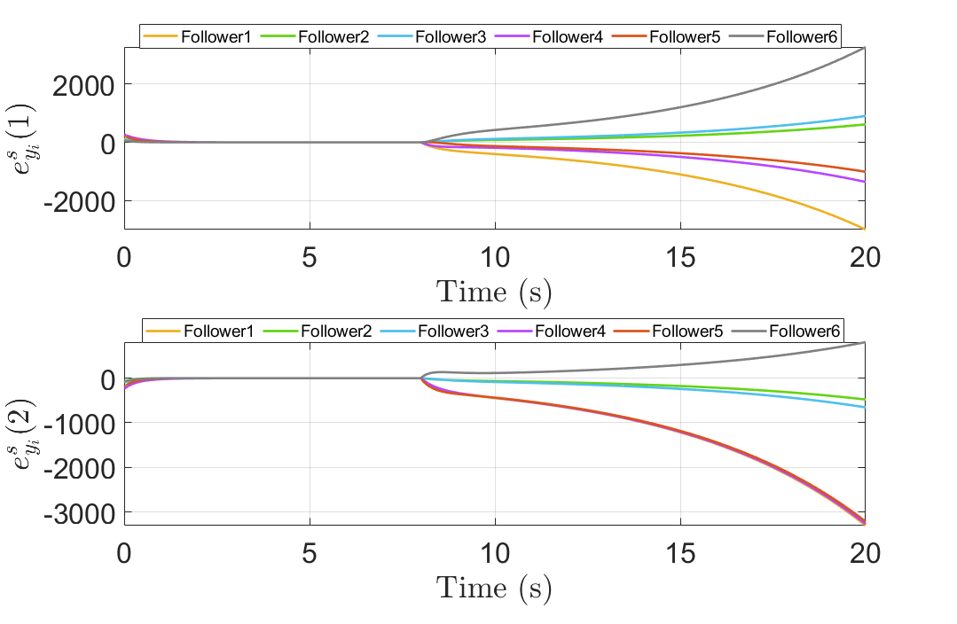
Figure 3: Bipartite output containment errors $e^{s}_{y_{i}}$ using the standard control protocols: $e^{s}_{y_{i}}(1)$ is the $x$ coordinate of $e^{s}_{y_{i}}$, $e^{s}_{y_{i}}(2)$ is the $y$ coordinate of $e^{s}_{y_{i}}$.

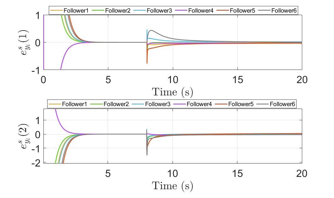
Figure 4: Bipartite output containment errors $e^{s}_{y_{i}}$ using the proposed resilient control protocols: $e^{s}_{y_{i}}(1)$ is the $x$ coordinate of $e^{s}_{y_{i}}$, $e^{s}_{y_{i}}(2)$ is the $y$ coordinate of $e^{s}_{y_{i}}$.

Based on Lemma 4, the bipartite output containment error in (12) serves to characterize the containment performance of the followers. Fig. 3 shows the evolution of the bipartite output containment errors using the standard bipartite containment control protocols described by (41). As seen, the bipartite output containment errors diverge due to the EU-FDI attacks after $8$ s. Fig. 4 shows the evolution of the bipartite output containment errors using the proposed resilient control protocols. As seen, after injecting the EU-FDI attacks at $8$ s, $e^{s}_{y_{i}}$ stays UUB for each follower, which shows that the UUB convergence performance is achieved under EU-FDI attacks.

Fig. LABEL:fig:_Leader-follower_motion_evolution_without_a_resilient_controller. shows the leader-follower motion evolution using the standard bipartite output containment control protocols. The three hollow circles are the trajectories of the leaders. As shown in Fig. LABEL:fig:_Leader-follower_motion_evolution_without_a_resilient_controller. (b), before the attack initiation at $8$ s, the standard control protocols achieve the bipartite output containment control objective, where the followers converge to the convex hull spanned by the outputs and negative outputs of the 3 leaders. However, as seen in Fig. LABEL:fig:_Leader-follower_motion_evolution_without_a_resilient_controller. (c), the followers’ trajectories diverge and fail to achieve the ARBOC objective after the initiation of the EU-FDI attacks at $8$ s. Fig. LABEL:fig:_Leader-follower_motion_evolution_with_the_proposed_controller. shows the leader-follower motion evolution using the proposed resilient control protocols. As seen from Fig. LABEL:fig:_Leader-follower_motion_evolution_with_the_proposed_controller. (c), after the initiation of the EU-FDI attacks, the followers remain confined to a small neighborhood around the convex hull spanned by the outputs and negative outputs of the three leaders, which validates the enhanced resilient performance of the proposed cyber-physical defense strategies against EU-FDI attacks on both CPL and OL.

V Conclusion

This paper has proposed a fully-distributed attack-resilient bi-layer defense framework to address the ARBOC problem for heterogeneous MASs, in the presence of EU-FDI attacks on both CPL and OL. First, an attack-resilient dynamic compensator that utilizes neighborhood relative information exchanged on the OL has been designed to estimate he convex combinations of the states and negative states of the leaders. The resilient compensator effectively addresses the EU-FDI attacks on the OL. Then, based on the compensator’s state, a fully-distributed attack-resilient local controller has been developed to address additional EU-FDI attacks on local actuator. This bi-layer defense framework has been mathematically proven to preserve the UUB consensus and system stability against EU-FDI attacks on both OL and CPL through rigorous Lyapunov stability analysis. The enhanced resilience of the proposed cyber-physical defense strategies has been validated using comparative simulation case studies.

References

• [1] P. Shi and Q. Shen, “Cooperative control of multi-agent systems with unknown state-dependent controlling effects,” IEEE Transactions on Automation Science and Engineering, vol. 12, no. 3, pp. 827–834, 2015.
• [2] L. Martinović, Žarko Zečević, and B. Krstajić, “Cooperative tracking control of single-integrator multi-agent systems with multiple leaders,” pp. 232–239, 2022. [Online]. Available: https://www.sciencedirect.com/science/article/pii/S0947358021001308
• [3] Y. Sun and Y. Shi, “Adaptive self-triggered control-based cooperative output regulation of heterogeneous multi-agent systems under sensor and actuator attack,” Proceedings of the Institution of Mechanical Engineers, Part I: Journal of Systems and Control Engineering, 2023, dOI: https://doi.org/10.1177/09596518231182288.
• [4] X.-G. Guo, D.-Y. Zhang, J.-L. Wang, J. H. Park, and L. Guo, “Observer-based event-triggered composite anti-disturbance control for multi-agent systems under multiple disturbances and stochastic fdias,” IEEE Transactions on Automation Science and Engineering, vol. 20, no. 1, pp. 528–540, 2022.
• [5] S. Knorn, Z. Chen, and R. H. Middleton, “Overview: Collective control of multiagent systems,” IEEE Transactions on Control of Network Systems, vol. 3, no. 4, pp. 334–347, 2015.
• [6] L. Wang, Z. Wang, K. Gumma, A. Turner, and S. Ratchev, “Multi-agent cooperative swarm learning for dynamic layout optimisation of reconfigurable robotic assembly cells based on digital twin,” Journal of Intelligent Manufacturing, pp. 1–24, 2024.
• [7] S. Wasserman and K. Faust, “Social network analysis: Methods and applications,” 1994.
• [8] J. Qin, W. Fu, W. X. Zheng, and H. Gao, “On the bipartite consensus for generic linear multiagent systems with input saturation,” IEEE Transactions on Cybernetics, vol. 47, no. 8, pp. 1948–1958, 2016.
• [9] P. Jayaraman, K. Devarajan, T. K. Chua, H. Zhang, E. Gunawan, and C. L. Poh, “Blue light-mediated transcriptional activation and repression of gene expression in bacteria,” Nucleic acids research, vol. 44, no. 14, pp. 6994–7005, 2016.
• [10] S. Zhai and W. X. Zheng, “On survival of all agents in a network with cooperative and competitive interactions,” IEEE Transactions on Automatic Control, vol. 64, no. 9, pp. 3853–3860, 2019.
• [11] Z. Gao, J. Pi, Y. Cai, and J. Gu, “Distributed finite-time bipartite containment control for heterogeneous fractional-order multi-agent systems,” in 2022 First International Conference on Cyber-Energy Systems and Intelligent Energy (ICCSIE). IEEE, 2023, pp. 1–5.
• [12] S. Zuo, Y. Song, F. L. Lewis, and A. Davoudi, “Bipartite output containment of general linear heterogeneous multi-agent systems on signed digraphs,” IET Control Theory & Applications, vol. 12, no. 9, pp. 1180–1188, 2018.
• [13] M. S. Chong, H. Sandberg, and A. M. Teixeira, “A tutorial introduction to security and privacy for cyber-physical systems,” in 2019 18th European Control Conference (ECC). IEEE, 2019, pp. 968–978.
• [14] L. Chen, L. Shi, Y. Cheng, and J. Shao, “Bipartite containment control for general linear multiagent systems under denial-of-service attacks,” in 2021 International Conference on Security, Pattern Analysis, and Cybernetics (SPAC). IEEE, 2021, pp. 495–500.
• [15] X. Wu, “Bipartite containment control for delayed multiagent systems with markovian switching topologies under impulsive attacks,” IEEE Access, 2023.
• [16] D. Jiang, G. Wen, Z. Peng, T. Huang, and A. Rahmani, “Fully distributed dual-terminal event-triggered bipartite output containment control of heterogeneous systems under actuator faults,” IEEE Transactions on Systems, Man, and Cybernetics: Systems, vol. 52, no. 9, pp. 5518–5531, 2021.
• [17] X. Wang, Y. Cao, B. Niu, and Y. Song, “A novel bipartite consensus tracking control for multiagent systems under sensor deception attacks,” IEEE Transactions on Cybernetics, 2022.
• [18] Y. Zhao, F. Zhu, and D. Xu, “Self-triggered bipartite formation-containment control for heterogeneous multi-agent systems with disturbances,” Neurocomputing, p. 126382, 2023.
• [19] J. Cheng, X. Zhan, J. Wu, T. Han, and H. Yan, “Adaptive bipartite output containment control of heterogeneous multi-agent systems with leaders bounded unknown inputs,” Neurocomputing, vol. 556, p. 126699, 2023.
• [20] S. Zuo, Y. Wang, M. Rajabinezhad, and Y. Zhang, “Resilient containment control of heterogeneous multi-agent systems against unbounded attacks on sensors and actuators,” IEEE Transactions on Control of Network Systems, 2023, dOI: https://doi.org/10.1109/TCNS.2023.3338772.
• [21] D. Widder, Advanced Calculus: Second Edition. Dover Publications, 2012. [Online]. Available: https://books.google.com/books?id=JWHtAAAAQBAJ
• [22] M. E. Valcher and P. Misra, “On the consensus and bipartite consensus in high-order multi-agent dynamical systems with antagonistic interactions,” Systems & Control Letters, vol. 66, pp. 94–103, 2014.
• [23] R. Rockafellar, Convex Analysis. Princeton University Press, 2015.
• [24] H. Khalil, Nonlinear Systems, 3rd ed. Prentice Hall, 2002.
• [25] F. L. Lewis, H. Zhang, K. Hengster-Movric, and A. Das, Cooperative control of multi-agent systems: optimal and adaptive design approaches. Springer Science & Business Media, 2013.
• [26] J. Huang, Nonlinear output regulation: theory and applications. SIAM, 2004.
• [27] H. Haghshenas, M. A. Badamchizadeh, and M. Baradarannia, “Containment control of heterogeneous linear multi-agent systems,” Automatica, vol. 54, pp. 210–216, 2015.
• [28] M. Krstic, P. V. Kokotovic, and I. Kanellakopoulos, Nonlinear and adaptive control design. John Wiley & Sons, Inc., 1995.