Pushing the Envelope of Low-Bit LLM via Dynamic Error Compensation

Abstract

Quantization of Large Language Models (LLMs) has recently gained popularity, particularly for on-device settings with limited hardware resources. While efficient, quantization inevitably degrades model quality, especially in aggressive low-bit settings such as 3-bit and 4-bit precision. In this paper, we propose QDEC, an inference scheme that improves the quality of low-bit LLMs while preserving the key benefits of quantization: GPU memory savings and inference latency reduction. QDEC stores the residual matrix—the difference between full-precision and quantized weights—in CPU, and dynamically fetches the residuals for only a small portion of the weights. This portion corresponds to the salient channels, marked by activation outliers, with the fetched residuals helping to correct quantization errors in these channels. Salient channels are identified dynamically at each decoding step by analyzing the input activations—this allows for the adaptation to the dynamic nature of activation distribution, and thus maximizes the effectiveness of error compensation. We demonstrate the effectiveness of QDEC by augmenting state-of-the-art quantization methods. For example, QDEC reduces the perplexity of a 3-bit Llama-3-8B-Instruct model from 10.15 to 9.12—outperforming its 3.5-bit counterpart—while adding less than 0.0003% to GPU memory usage and incurring only a 1.7% inference slowdown on NVIDIA RTX 4050 Mobile GPU. The code will be publicly available soon.

1 Introduction

Recent advancements in Large Language Models (LLMs) based on the Transformer architecture [58] have shown great potential to reshape various aspects of our daily lives [1, 55, 43, 39, 54]. However, their deployment costs, largely due to their substantial size, present a significant barrier to broader accessibility. The large model size increases memory requirements, driving up system costs, and also results in longer inference latencies, thereby limiting potential use cases [59].

Quantization has gained attention as a promising solution for mitigating the deployment costs of LLMs [68, 27]. By lowering the precision of model parameters, quantization addresses both memory limitations and inference latency. The importance of quantization is especially pronounced for on-device deployments, where model compression is often a necessity rather than an option due to strict memory budgets. In such scenarios, it is a common practice to explore the trade-off between model size and quality by adjusting the quantization levels, in order to find the most effective solution within the given memory constraints [15, 14, 60, 8, 57].

While quantization may allow gigantic LLMs to fit into small-memory devices—something that would have been impossible otherwise—it often leads to model quality degradation due to the inevitable loss of information. This is especially true for low-bit settings, such as 3-bit and 4-bit quantization, which are often used to accommodate the parameter sizes of LLMs [30, 35, 19]. This raises a key research question that this paper addresses: given a quantized LLM configured with the best possible effort under the memory budget, is there a way to recover the quality loss caused by quantization?

Leveraging external memory offers a potential solution to this problem. Specifically, on heterogeneous computing platforms where the CPU and GPU are connected via a PCIe interconnect—a common architecture in desktops and laptops—CPU memory becomes a viable option. Additional information that may be used to mitigate quantization errors can be stored in CPU memory and fetched at runtime, avoiding any additional GPU memory overhead.

However, utilizing CPU memory for GPU inference presents a critical challenge: the slow data transfer between the CPU and GPU can create a bottleneck for inference latency. To mitigate this issue, the volume of data transferred must be carefully controlled. Therefore, designing a system that effectively utilizes CPU memory requires the identification of the minimal set of additional information that can substantially enhance the quality of quantized models, while keeping the impact on latency minimal.

A clue for this problem comes from the well-known fact that not all channels in the weight matrix are equally important for weight quantization. Some channels, referred to as salient channels, are more critical, primarily due to the presence of activation outliers [10, 7, 24]. When certain input activation values are particularly large, the quantization errors in the corresponding weight channels—those multiplied by these large activation values—are amplified, making the channels salient. By identifying these channels and selectively fetching error compensation terms from CPU memory, we can maximize the quality boost while minimizing data transfer.

Hence, the accurate identification of these salient channels is essential for overcoming the limited communication bandwidth, allowing for the transfer of only impactful information. Previous works that attempt to improve quantization algorithms by addressing activation outliers often analyze the distribution of activation values on a calibration dataset to predetermine the salient channels [10, 32, 26, 35]. However, this approach is suboptimal because it statically designates certain weight channels as salient throughout the inference, while the real distribution of activation values—and thus the distribution of salient channels—changes dynamically at each decoding step. Accounting for the dynamic nature of activation outliers is crucial for the accurate identification of salient channels.

Thus, in this paper, we introduce QDEC (Quantization with Dynamic Error Compensation), an inference scheme for quantized LLMs that dynamically identifies salient channels and compensates for quantization errors in these channels, in real time. QDEC enhances model quality while fully preserving the two main benefits of quantization, namely reduced GPU memory usage and improved inference latency, by efficiently utilizing CPU memory. To achieve this, QDEC stores the residuals of the quantized weight matrices in CPU memory, fetching only the parts that correspond to the dynamically identified salient channels for error compensation. Although small in size, these residuals provide a significant quality boost. This dynamic error compensation is performed concurrently with inference by a highly optimized GPU kernel, ensuring that all additional operations are seamlessly integrated into the existing workflow, thereby minimizing any inference slowdown. Below are the key contributions of our work:

• We provide an in-depth analysis on the dynamic nature of activation outliers in LLM inference.

• We present QDEC, an inference scheme that enhances quantized LLMs by dynamically identifying salient channels and compensating quantization errors in them.

• We introduce a parameter tuner for QDEC that automatically recommends system parameters to satisfy a target latency bound.

• We provide a comprehensive evaluation of QDEC across five different consumer-grade GPUs, demonstrating significant quality improvement with minimal memory and inference latency overhead.

2 Background

Figure 1: LLM inference.

2.1 LLM Inference

Figure 1 presents a description of the modern LLM architecture and its inference flow. LLMs consist of multiple Transformer decoder blocks [58], each containing multiple linear layers, which account for most of the inference time, alongside other components like self-attention and normalization.

LLM inference involves two phases: prefill and decode. In the prefill phase, all input tokens (e.g., ’I’, ’am’, ’a’) are processed in parallel to generate a single output token (e.g., ’computer’). The decode phase begins subsequently, where the output token of the previous step is fed back into the model to generate the next token, repeated until the end of the sequence. This sequential nature of the decode phase makes it the primary latency bottleneck.

The decode phase is particularly memory-bound, as only one token is processed at a time, reducing the linear layers to GEMV operations. In data center settings, this issue can be alleviated by batching together multiple queries [65, 31]. However, this usually cannot be applied to on-device inference, where LLMs serve only individual users.

2.2 LLM Quantization

Quantization for LLMs—a popular compression technique that reduces both memory usage and inference latency—can be categorized into two main types [68, 27]: weight-activation quantization [64, 10, 48, 63, 36, 33] and weight-only quantization [19, 35, 30, 12, 32, 9, 56, 17, 11, 29]. Each are suited to different inference scenarios. Weight-activation quantization is primarily used in datacenter settings, where both memory and computational costs must be minimized to improve throughput. Quantizing both weights and activations allows for the efficient use of low-precision arithmetic units (e.g., INT4, INT8, FP8) available on modern GPUs [2]. In contrast, for on-device inference, weight-only quantization is the preferred approach [68, 30]. In this apporach, quantized weights are loaded from memory and dequantized on-the-fly to full precision (i.e., FP16), before being multiplied with the full-precision activations [44]. While this reduces only the memory bandwidth and not the computation, the memory reduction alone is sufficient to achieve speedups in on-device inference, where memory bandwidth is the primary bottleneck, as discussed in Section 2.1.

Weight-only quantization can be further divided into two sub-categories: quantization-aware training (QAT) [36, 11, 29], and post-training quantization (PTQ) [19, 35, 30, 12, 32, 9, 56, 17]. While QAT, which mitigates quantization errors through retraining, typically yields better results, the high costs of retraining make it impractical for many end-users [30, 68]. As a result, PTQ, which does not require retraining, has become the preferred quantization method for on-device LLM inference. Therefore, in this paper, we specifically focus on weight-only PTQ for on-device inference.

3 Augmenting Quantized LLM with CPU Memory

In this section, we propose leveraging CPU memory—an often underutilized resource in LLM inference, as GPUs are the de facto standard processors for this workload—as a means to augment quantized LLMs. Section 3.1 introduces the concept of CPU-augmented quantized LLM while Section 3.2 and Section 3.3 explore its opportunities and challenges.

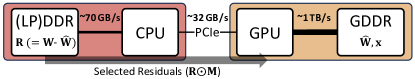
Figure 2: CPU-augmented inference system for quantized LLMs.

3.1 Concept

Goal. We aim to utilize CPU memory as a means to enhance the quality of quantized LLMs without additional GPU memory costs. In model quantization, there is an inherent trade-off between size and quality: the more memory you allocate, the higher the quality you can achieve. When deploying quantized models in resource-constrained environments, it is common practice to explore this trade-off and determine the optimal bitwidth under the target GPU memory budget. This process can be a simple selection of a bitwidth to be uniformly applied to all parameters, or a more fine-grained allocation of bitwidths, such as layer-wise [15, 14, 8] or channel-wise [60, 57]. CPU memory may come into play once this process is complete, enabling further improvements without consuming additional GPU memory.

Basic Mechanism. Figure 2 illustrates our concept of leveraging CPU memory to enhance quantized LLMs. We primarily target desktop or laptop platforms, where the GPU is connected to the CPU via a PCIe interconnect. As in conventional inference systems, the quantized weight parameters ($\widehat{\mathbf{W}}$) and activations ($\mathbf{x}$) are kept in GPU memory. The difference here is that $\mathbf{R}$—the residual between the original full-precision weights and the quantized weights—is stored in CPU memory. During the decode phase, residuals are fetched from the CPU to help compensate for quantization errors, potentially improving model quality. Due to the limited bandwidth of PCIe, which is typically an order of magnitude lower than GPU memory bandwidth (e.g., 32 GB/s vs. 1 TB/s), fetching the entire residual matrix would incur a prohibitive latency bottleneck. Therefore, only a small subset of residuals should be fetched in a selective manner. In short, this process augments each linear operation of quantized LLM from $\widehat{\mathbf{W}}\mathbf{x}$ to $(\widehat{\mathbf{W}}+\mathbf{R\odot M})\mathbf{x}$, where $\mathbf{M}$ is a binary mask that sparsifies $\mathbf{R}$.

Key Research Question. A key research question in designing an effective CPU-augmented inference system for quantized LLMs is determining a proper subset of residuals, or mask $\mathbf{M}$. A good mask $\mathbf{M}$ should: 1) select portions of the residuals that contribute most to improving model quality within the given bandwidth constraints, and 2) maintain a structured form that minimizes indexing overhead, thereby maximizing the effective transfer of residuals, while ensuring efficient processing on the GPU.

Figure 3: Activation outlier issue in weight quantization.

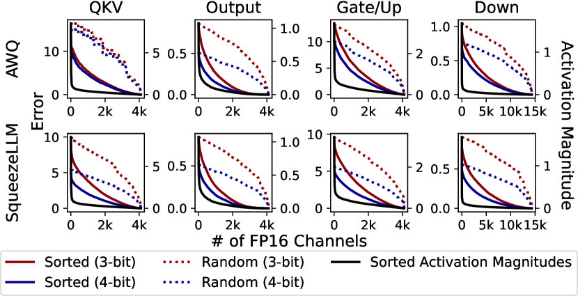
Figure 4: Quantization error reduction trends observed when replacing the input channels of quantized weights with FP16 values sequentially in sorted order (solid lines) and random order (dotted lines) for the 16th decoder block of Llama-3-8B-Instruct. The distribution of activation magnitudes in sorted order is also shown (black lines).

Figure 5: (a) Distribution of activation outliers (top 5%) and (b) Recall rate of static analysis-based outlier identification for the true top 1% and 5% outliers, across 100 decoding steps. The 16^th decoder block’s down projection of Llama-3-8B-Instruct model is used for profiling.

3.2 Opportunity: Not All Residuals Are Equally Important

Some residuals are more important than others—an opportunity that can be leveraged to determine $\mathbf{M}$. This opportunity arises from the presence of activation outliers (i.e., activation values with large magnitudes), a well-known phenomenon in LLM inference [10, 32, 35, 26, 7, 24]. When certain activation values are noticeably large, even small quantization errors in the corresponding weight channels can be multiplied and amplified, leading to considerable perturbations in the output. Figure 3 illustrates this issue. In this example, the third input channel (third row) of the weight matrix is multiplied by the activation outlier, -3.0. We refer to such channels as salient channels. Constructing $\mathbf{M}$ at the input channel granularity based on the magnitude of input activations can satisfy two key conditions for an effective mask: selecting impactful portions of the residuals and maintaining a structured form.

Indeed, compensating for errors in salient channels using the corresponding residuals is highly effective. Figure 4 illustrates how the quantization error, defined as the mean square error between the computation result with FP16 weights (${\mathbf{W}}\mathbf{x}$) and quantized weights ($\widehat{\mathbf{W}}\mathbf{x}$), is reduced by sequentially replacing the input channels of the quantized weight with their corresponding FP16 values. For this analysis, 3-bit and 4-bit models of the Llama-3-8B-Instruct model [16], quantized using two state-of-the-art methods, AWQ [35] and SqueezeLLM [30], are evaluated. Specifically, the 7th decoding step is analyzed with the input prompt: "What are large language models?". All four linear layers in the 16th decoder block are included in this evaluation. The quantization errors for both 3-bit and 4-bit models are rapidly reduced when progressively compensating for channels in descending order of the corresponding activation magnitudes (solid red and solid blue lines). This trend closely follows the activation magnitude distribution (solid black line), which represents the sorted activation magnitudes in descending order. In contrast, the reduction in quantization error is significantly slower when input channels are compensated in random order, as shown by the dotted lines. This highlights the importance of prioritizing salient channels based on activation magnitude.

3.3 Challenge: Dynamic Nature of Activation Outliers

Identifying salient channels is challenging because the distribution of activation outliers changes dynamically by nature. While it is possible to infer salient channels by statically analyzing activation value statistics on a small calibration set [10, 32, 26, 35], such static approaches are suboptimal. Figure 5(a) shows the distribution of activation outliers—defined as activations with the top 5% magnitudes—in the down projection layer of the 16^th decoder block of the Llama-3-8B-Instruct model over 100 decoding steps, again using the input prompt: "Large language models are". For better visibility, only the first 1024 channels are displayed. While some channels (e.g., Channel 421, highlighted by an arrow) consistently exhibit high activation magnitudes and remain persistent outliers, the distribution of activation outliers generally shows significant irregularity across different decoding steps.

To quantify the dynamic nature of activation outliers, we calculate the recall rate of the top 1% and top 5% outliers identified through static analysis using a calibration set, compared to the true top 1% and top 5% outliers (ground truth) observed at each decoding step. We use a subset of the Pile dataset [21] for calibration, following prior work [35]. Specifically, we profile the average of the mean square of each activation value and use this as a metric for identifying outliers. Figure 5(b) presents the results, showing that the recall rate remains low ($\sim$20%) for both the top 1% and top 5% outliers. This highlights a clear limitation of static analysis, as it misses the majority of outliers at runtime, emphasizing the need for dynamic identification of salient channels.

4 QDEC Design

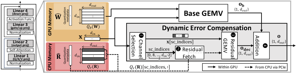
Figure 6: QDEC overview.

4.1 Overview

In this section, building on the opportunity outlined in Section 3.2 and addressing the challenge described in Section 3.3, we propose QDEC, a CPU-augmented inference system for quantized LLMs that performs decoding with dynamic error compensation. Figure 6 presents an overview of QDEC. During the decode phase, QDEC augments each linear layer, essentially a GEMV operation, with dynamic error compensation. Specifically, to produce the final output ($\mathbf{o}$), QDEC adds an error compensation term ($\mathbf{o_{\text{dec}}}$) to the result of the base GEMV, $\mathbf{o_{\text{b}}}$, which is obtained by multiplying the input vector ($\mathbf{x}$) with the quantized weights ($\mathbf{\widehat{W}}$). $\mathbf{o_{dec}}$ is computed by multiplying the input vector with a subset of weight residuals selectively fetched from the CPU. This selection of weight residuals is performed dynamically, fully accounting for the changing distribution of input vectors. To maximize the number of residual values fetched under PCIe bandwidth constraints, QDEC stores and retrieves a quantized version of the residuals ($\mathbf{\widehat{R}}$), comprising the quantized values $Q_{r}(\mathbf{R})$ and associated metadata, instead of the full-precision residuals ($\mathbf{R}$). Here, $Q_{r}$ is a quantizer function for residuals that maps full-precision values to low-bit representations. Note that $Q_{r}$ is distinct from the quantizer function used for the original weight quantization, or base quantizer function, $Q_{b}$.

The dynamic error compensation process consists of four sequential steps. First, by investigating the input activation vector, QDEC creates sc_indices, a list of salient channel indices. The number of salient channels to compensate, $k$, is a preconfigured parameter. This step is essentially a Top-K operation that selects the values in the input activation vector with the largest magnitudes. Next, a portion of the quantized residuals corresponding to the salient channels, $Q_{r}(\mathbf{R})[\texttt{sc\_indices},:]$ (along with the necessary quantization metadata), is fetched from the CPU via PCIe. The fetched residuals are then multiplied by the sparsified activation vector ($\mathbf{x}[\texttt{sc\_indices}]$), producing $\mathbf{o_{dec}}$. Finally, the resultant $\mathbf{o_{dec}}$ is added to the base GEMV result $\mathbf{o_{b}}$, producing the final output, $\mathbf{o}$. All the operations of the dynamic error compensation process are performed in parallel with the base GEMV on a different GPU stream, and must be highly efficient to remain hidden within the base GEMV execution time.

The following sections provide details of each component of QDEC. Section 4.2 explains how QDEC performs the residual quantization. Section 4.3 details the GPU implementation of the dynamic error compensation. Section 4.4 illustrates how QDEC configures system parameters, including $k$, the number of channels to compensate.

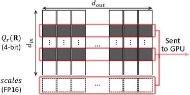
Figure 7: Quantization of weight residual.

4.2 Residual Quantization

Figure 7 depicts the quantization scheme for the residuals. QDEC employs 4-bit quantization for each output channel (i.e., column) of the residuals. To minimize metadata, symmetric uniform quantization is used. This approach requires only a single scalar scale factor as metadata for each output channel. The residual quantizer for the $i$-th output channel ($Q_{r,i}$) is defined as:

$$Q_{r,i}(r)=\text{clip}\left(\text{round\_to\_int}\left(\frac{r}{S_{i}}\right),-7,7\right).$$

$S_{i}$, the scale factor, is determined through a grid search as the value that minimizes the mean squared error between the original and quantized weights.

Using this quantizer, each floating-point residual value $r$ is projected to an integer between -7 and 7. At runtime, the selected input channels of the quantized residuals (highlighted in Figure 7) and all the scale factors are fetched from the CPU. Each input channel of the quantized residuals, as well as the scales, are stored contiguously in CPU memory, enabling coalesced data transfers.

4.3 Efficient Implementation of Dynamic
Error Compensation

The top priority in implementing dynamic error compensation is ensuring low latency, allowing its execution to remain hidden within the base GEMV execution time. To fetch a sufficient number of residual channels within this short time window, QDEC introduces three key software optimization strategies: 1) zero-copy residual fetching, 2) fast approximate Top-K for channel selection, and 3) kernel fusion.

Zero-Copy Residual Fetch. QDEC leverages CUDA zero-copy [41], instead of commonly used API functions such as cudaMemcpy() or cudaMemcpyAsync(), to fetch the residuals from CPU. These APIs rely on the direct memory access (DMA) engine for data transmission, which is efficient at transferring large data blocks but suboptimal for smaller transfers due to the DMA setup overheads. Fetching residuals, however, falls into the latter category. The granularity of residual fetching occurs at the row level of the quantized residual matrix. With 4-bit quantization and typical row lengths of a few thousand to tens of thousands, each data block transfer is only a few tens of KBs. For optimal PCIe bandwidth utilization, the data block size should ideally be at least a few hundred KBs (e.g., 256 KB) [40, 46]. In zero-copy access, the GPU directly sends cacheline-sized memory requests, making it suitable for fine-grained data access. While zero-copy access has the disadvantage of occupying GPU cores to generate memory requests—potentially slowing down other concurrently running kernels—this is not a major issue for QDEC. The concurrent kernel for our case, the base GEMV, is typically memory-bound, so using fewer cores for this kernel is unlikely to have significant impact on its execution time.

Figure 8: Fast approximate Top-K operation of QDEC.

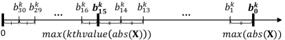
Figure 9: Bucket boundaries used in the approximate Top-K operation of QDEC.

Fast Approximate Top-K for Channel Selection. For channel selection, QDEC employs an approximate Top-K method that is fast and GPU-friendly, while maintaining sufficient precision. This approach avoids the latency overhead of an exact Top-K operation. Figure 8 explains the approximation by providing an example where 128 elements need be selected from a 4096-dimensional input activation vector ($d_{in}=4096$, $k=128$). As shown in Figure 8(a), instead of performing one global selection over the entire input vector, QDEC conducts multiple local searches, one for each contiguous 1024-dimensional subvector, or chunk. For each chunk, $k_{chunk}$ elements are selected, where $k_{chunk}$ is $k$ divided by the number of chunks. In this example, we have four chunks, and $k_{chunk}$ is 32. The results from each local search are concatenated to form the final result. While this approach introduces approximation, it significantly reduces latency by eliminating the global synchronization, as each local search can be handled independently by a separate thread block.

For each local search, QDEC uses a variant of the bucket-based Top-K algorithm [3]. Figure 8(b) illustrates this process. First, the 1024 elements in a chunk are scattered into buckets based on their magnitudes, with bucket boundaries ($b^{k}_{0}$, $b^{k}_{1}$, …, $b^{k}_{30}$). The number of buckets is set to 32, matching the number of threads in a warp, allowing for efficient thread-level parallelism so that each thread processes a different bucket. Next, elements are gathered, starting from bucket 0, until the total count reaches $k_{chunk}$. If the number of elements in the current bucket exceeds the remaining spots for $k_{chunk}$, as in the case of bucket 9 in Figure 8(b), random selection is used to fill the remaining spots. This random selection adds an additional layer of approximation but significantly reduces latency by avoiding exact sorting.

Determining proper bucket boundaries is crucial for minimizing the approximation error introduced by random selection ( in Figure 8(b)). QDEC profiles the distribution of activation values using a small calibration set and aims to set boundary values that balance Top-K accuracy with the ability to handle a broader range of values. Placing finer-grained buckets around the expected $k$-th largest value generally improves accuracy, but it limits the system’s ability to handle out-of-distribution values. To address this, QDEC uses an offline analysis to determine two key boundaries, $b^{k}_{0}$ and $b^{k}_{15}$, from which the other boundaries are inferred (as shown in Figure 9). Assume the distribution of activation values from the calibration set is $\mathbf{X}\in R^{N\times d_{in}}$, where $N$ is the size of the set. The boundary $b^{k}_{15}$ is set to the maximum of the $k$-th largest value across all vectors in $abs(\mathbf{X})$. The interval between 0 and $b^{k}_{15}$ is uniformly divided into 16 buckets ($b^{k}_{15}$, $b^{k}_{16}$, …, $b^{k}_{30}$), focusing on the range where the $k$-th largest value is most likely to occur. To handle out-of-distribution cases which can cause significant degradation in selection precision, QDEC assigns an additional 16 buckets for values beyond $b^{k}_{15}$. Specifically, $b^{k}_{0}$ is set to the maximum value in the entire $abs(\mathbf{X})$, and the range between $b^{k}_{0}$ and $b^{k}_{15}$ is also uniformly divided to form the remaining 16 buckets.

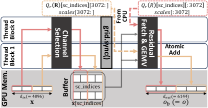
Figure 10: Fused kernel for dynamic error compensation.

Kernel Fusion. QDEC extensively fuses all dynamic error compensation operations into a single kernel. Figure 10 visualizes the execution flow of the fused kernel, using an example where two thread blocks process a weight matrix of size 4096$\times$6144. In this example, only one channel is selected per each of the four chunks (i.e., $k_{chunk}=1$, $k=4$). Initially, each thread block sequentially processes two chunks, selecting a total of two channels (Step in Figure 6(b)). The indices for the selected channels (sc_indices) as well as the corresponding activation values ($\mathbf{x}[\texttt{sc\_indices}]$) are stored in GPU memory. Thread blocks are then synchronized using the grid-wide synchronization feature of the cooperative group [42]. This synchronization is necessary because, when fetching quantized residuals from the CPU and performing GEMV with the fetched data (Steps and in Figure 6(b)), each thread block handles a segment of every selected channel, rather than only a specific subset of selected channels. For example, thread block 0 processes $Q_{r}(\mathbf{R})[\texttt{sc\_indices}][:3072]$ as opposed to $Q_{r}(\mathbf{R})[\texttt{sc\_indices}[:2]][:]$. The thread block-level synchronization allows all thread blocks to have access to the complete set of sc_indices and $\mathbf{x}[\texttt{sc\_indices}]$. This partitioning scheme allows for efficient reduction in the residual GEMV without requiring extensive global synchronization. The results from the residual GEMV are directly added to the result of the base GEMV ($\mathbf{o_{b}}$) using atomic primitives, yielding the final output ($\mathbf{o}$) (Step in Figure 6(b)).

GPU Memory Overhead. The buffer for sc_indices and $\mathbf{x}[\texttt{sc\_indices}]$ in the fused kernel is the only additional GPU memory usage of QDEC. Zero-copy from the CPU does not consume GPU memory. The bucket boundary values are not stored on the GPU; instead, only $b^{k}_{0}$ and $b^{k}_{15}$ are passed to the kernel as arguments. A single buffer can be reused for all linear layers if it is sized in accordance with the largest $k$. In the extreme case of fetching 10% of the channels across all layers in Llama-3-8B, the maximum $k$ would be 1433, for the down projection layer. This calls for an 8.6 KB buffer ($1433\times(4+2)$), which is less than 0.0003% of the model size, assuming 3-bit precision—essentially a negligible overhead.

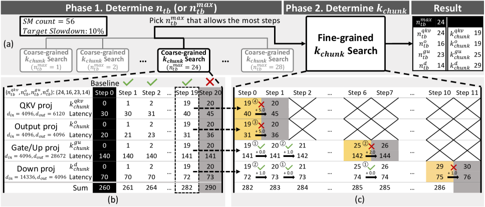
Figure 11: Parameter tuning process for QDEC, assuming a total of 56 SMs and a target slowdown rate of 10%.

4.4 Parameter Tuner

Necessity of Parameter Tuner. To effectively utilize QDEC, two key parameters must be carefully tuned. The first is the ratio of input channels to compensate in each layer, controlled by $k_{chunk}$, which denotes the number of input channels to compensate per 1024 input channels. A larger $k_{chunk}$ improves model quality but may increase inference latency. The second is $n_{tb}$, the number of thread blocks allocated for the dynamic error compensation. Since the dynamic error compensation runs in parallel with the base GEMV, assigning too many thread blocks to it can slow down the base GEMV. On the other hand, if too few thread blocks are assigned, the PCIe bandwidth cannot be fully utilized, as the zero-copy mechanism relies on GPU cores to issue memory requests.

Determining $k_{chunk}$ and $n_{tb}$ requires significant effort due to the vast design space. The value of $k_{chunk}$ for each type of linear layer in a decoder block ($k^{qkv}_{chunk}$, $k^{o}_{chunk}$, $k^{gu}_{chunk}$, $k^{d}_{chunk}$) can be any integer less than its maximum possible value, which is constrained by the shared memory size. While this maximum may vary across platforms, it is typically quite large (e.g., 367 in the NVIDIA Ada architecture), resulting in an expansive search space. Meanwhile, $n_{tb}$ values for each layer ($n^{qkv}_{tb}$, $n^{o}_{tb}$, $n^{gu}_{tb}$, $n^{d}_{tb}$) are constrained by the input and output dimensions of the weights, leading to far fewer possible candidates compared to $k_{chunk}$. Still, however, each layer has multiple viable candidate values. For example, in Llama-3-8B, there are 9 possible candidates for $n^{qkv}_{tb}$ (1, 2, 3, 4, 5, 6, 8, 12, 24), while other layers also have multiple options. This leads to a combinatorial explosion in the number of possible configurations. We provide details about identifying possible values for $k_{chunk}$ and $n_{tb}$ in the supplementary material.

To ease this process, we provide a parameter tuner for QDEC, which suggests values for $k_{chunk}$ and $n_{tb}$ based on the user’s target slowdown rate. Specifically, the tuner seeks to maximize $k_{chunk}$ values while ensuring that the total execution time—including the base GEMV and the dynamic error compensation across all linear layers in the block—remains within the target slowdown rate compared to the baseline execution time without dynamic error compensation. This parameter tuning is a one-time process for a given model-device pair.

Paramter Tuning Process. Figure 11(a) illustrates the tuning process, which consists of two phases: Phase 1 determines the $n_{tb}$ values, and Phase 2 determines the $k_{chunk}$ values.

In Phase 1, the tuner simplifies the search for $n_{tb}$ values for each layer by replacing it with the search for a single metaparameter, $n^{max}_{tb}$. $n^{max}_{tb}$ represents the upper limit on the number of thread blocks to use for dynamic error compensation. Once the $n^{max}_{tb}$ value is determined, the $n_{tb}$ values for each layer are set to the largest possible candidate value smaller than $n^{max}_{tb}$. Determining $n^{max}_{tb}$ involves testing values up to half of the total SM count, rather than up to the total SM count, to reduce the search space. In the example shown in Figure 11, the GPU has 56 SMs, so values up to 28 are tested. Each test includes a coarse-grained search for $k_{chunk}$, which is to determine, for the given $n^{max}_{tb}$, how many steps can be taken when incrementing $k_{chunk}$ uniformly for all layers without exceeding the target slowdown rate. Figure 11(b) shows an example of a coarse-grained $k_{chunk}$ search for $n^{max}_{tb}=24$ (i.e., $(n^{qkv}_{tb},n^{o}_{tb},n^{gu}_{tb},n^{d}_{tb})=(24,16,23,14)$), where a total of 19 steps were made. If no steps can be made for any $n^{max}_{tb}$ value, the tuner fixes $k_{chunk}$ to 0 for the layer with the smallest weight matrix and repeats the process, as smaller matrices are often most sensitive to increases in $k_{chunk}$.

After Phase 1, the tuner selects the $n^{max}_{tb}$ that allows the most steps and proceeds to Phase 2, which involves a fine-grained $k_{chunk}$ search. Figure 11(c) illustrates this fine-grained $k$ search with the selected $n^{max}_{tb}$, which is 24 in this example. In this phase, not all $k_{chunk}$ values may increase together. At each step, the tuner increments $k_{chunk}$ for as many layers as possible, prioritizing those with smaller increases in execution time. For example, in Step 1, $k^{gu}_{chunk}$ is incremented first, followed by $k^{d}_{chunk}$. Step 1 stops at this point, as further increases to $k^{qkv}_{chunk}$ and $k^{o}_{chunk}$ would exceed the target; thus their final values are set (i.e., $k^{qkv}_{chunk},k^{o}_{chunk}=19$). This process repeats until no further increments can be made for any layer.

5 Evaluation

5.1 Methodology

Quantized LLMs. We evaluate the effectiveness of QDEC by integrating it on 3-bit, 3.5-bit and 4-bit versions of two instruction-tuned LLMs: Llama-3-8B-Instruct [16] and Phi-3-medium-4k-instruct (14B) [39]. For the 3.5-bit version, we adopt a block-wise bitwidth allocation, applying 3-bit quantization to half of the decoder blocks and 4-bit quantization to the remaining blocks. This allocation is guided by a Kullback–Leibler (KL) divergence-based sensitivity metric, as proposed in prior work [8]. As base quantization methods, we choose two state-of-the-art LLM quantization methods that excel in both model quality and inference latency: AWQ [35] and SqueezeLLM [30]. AWQ is a uniform quantization method that mitigates quantization errors by applying per-channel scaling to protect salient channels, which are identified through an offline analysis on a calibration dataset. SqueezeLLM employs a clustering-based non-uniform quantization method that considers the sensitivity of each weight.

Benchmarks. Following previous literature [9, 30, 35, 12], we use perplexity on the WikiText dataset [38] as a primary metric since perplexity reliably reflects the quality of quantized LLMs [35, 13]. Additionally, we use BIG-Bench Hard (BBH) [53], a collection of 23 challenging tasks in BIG-Bench [51], to assess the models’ capabilities in complex problem solving. Chain-of-Thought (CoT) prompting is enabled for all BBH evaluations [61]. Lastly, we evaluate multi-turn conversation using MT-Bench [67], where a strong LLM serves as a judge, scoring the model’s responses on 80 sample questions with integer scores ranging from 0 to 10. We use GPT-4o as the judge. For MT-Bench evaluation, we repeat the experiments three times and report the average score.

Figure 12: Perplexity on WikiText. The x markers correspond to baselines without QDEC ($k_{chunk}=0$). Lower is better.

Figure 13: Accuracy on BBH. The x markers correspond to baselines without QDEC ($k_{chunk}=0$). Higher is better.

Figure 14: MT-Bench scores. The x markers correspond to baselines without QDEC ($k_{chunk}=0$). Higher is better.

5.2 Impact on Model Quality

Methodology. In this section, we demonstrate the model quality improvements achieved by QDEC. We evaluate models with varying $k_{chunk}$, the number of channels compensated per chunk (1024 channels), uniformly setting it to 8, 16, 32, 64 and 128 for all layers.

Perplexity on WikiText. Figure 12 shows the perplexity results. Across all cases, a clear trend is observed: perplexity consistently decreases (i.e., model quality improves) as $k_{chunk}$ increases. Notably. for 3-bit models, significant drops in perplexity are achieved even with a low $k_{chunk}$ of 8. AWQ’s perplexity decreases from 10.15 to 9.63 for Llama-3 and from 5.96 to 5.53 for Phi-3, while SqueezeLLM’s perplexity drops from 10.49 to 9.93 for Llama-3 and from 5.92 to 5.45 for Phi-3. Meanwhile, the impact of dynamic error compensation on 4-bit models is relatively less pronounced. This is expected, as 4-bit models already offer high quality and are much closer to the full-precision models, leaving a smaller room for improvement. The 3.5-bit models exhibit trends that fall between those of the 3-bit and 4-bit models.

BBH and MT-Bench. Results on BBH (Figure 13) follow the same trends as the perplexity results. The MT-Bench results (Figure 14), on the other hand, demonstrate some different patterns. In cases where vanilla quantized models without QDEC ($k=0$) already achieve scores very close to those of the FP16 model—such as all 4-bit cases and the AWQ 3.5-bit model of Phi-3—the scores remain unchanged with QDEC, oscillating around the baseline score. For the remaining cases, QDEC significantly improves scores even with a small $k_{chunk}$ (e.g., 8), like in other benchmarks; further increases in $k_{chunk}$, however, do not always yield noticeable improvements. These patterns may be attributed to the coarse-grained rubric of this benchmark, which assigns integer scores ranging from 0 to 10 for each task. Such a scoring scheme may fail to capture the subtle improvements introduced by dynamic error compensation when the potential for improvement is limited.

Figure 15: Comparison against exact Top-K channel selection. line graphs show perplexity, and bar graphs represent the average recall rate of QDEC’s approximate Top-K.

Impact of Top-K Approximation. Figure 15 compares the perplexity between QDEC and QDEC with exact Top-K selection to investigate the impact of QDEC’s Top-K approximation. The average recall rate of QDEC’s approximate Top-K is also reported. In all cases, the approximation performs well, achieving a recall rate of around 80% and yielding perplexity nearly identical to the exact Top-K.

Figure 16: Comparison against static and random channel selection. Lower is better.

Impact of Dynamic Salient Channel Selection. To evaluate the impact of dynamic salient channel selection in QDEC, we compare its perplexity with its two variants: (1) compensating for errors in a static set of channels identified via calibration set analysis, and (2) compensating for errors in a random set of channels. For the static identification of salient channels, we use a Hessian-based metric following prior work [32]. Figure 16 shows the results. While QDEC with static channel selection outperforms random selection, it significantly falls short of the original dynamic QDEC. For example, to achieve a similar level of perplexity as QDEC with $k_{chunk}=64$, QDEC with static channel selection requires $k_{chunk}$ to be 256, making it impractical.

Llama-3-8B-Instruct

Phi-3-medium-4k-instruct

AWQ 3-bit

SqueezeLLM 3-bit

AWQ 3-bit

SqueezeLLM 3-bit

$k_{chunk}$

2-bit

4-bit

8-bit

FP16

2-bit

4-bit

8-bit

FP16

2-bit

4-bit

8-bit

FP16

2-bit

4-bit

8-bit

FP16

2

gray!40

gray!40

gray!40

red!309.83

gray!40

gray!40

gray!40

red!3010.10

gray!40

gray!40

gray!40

red!305.56

gray!40

gray!40

gray!40

red!305.63

4

gray!40

gray!40

red!309.72

orange!309.72

gray!40

gray!40

red!309.97

orange!309.97

gray!40

gray!40

red!305.51

orange!305.51

gray!40

gray!40

red!305.55

orange!305.56

8

gray!40

red!309.63

orange!309.58

yellow!309.58

gray!40

red!309.93

orange!309.79

yellow!309.78

gray!40

red!305.45

orange!305.45

yellow!305.45

gray!40

red!305.53

orange!305.47

yellow!305.47

16

red!309.63

orange!309.47

yellow!309.43

green!309.43

red!309.95

orange!309.75

yellow!309.59

green!309.58

red!305.47

orange!305.36

yellow!305.35

green!305.35

red!305.51

orange!305.44

yellow!305.36

green!305.37

32

orange!309.49

yellow!309.29

green!309.25

cyan!309.25

orange!309.80

yellow!309.54

green!309.36

cyan!309.36

orange!305.36

yellow!305.24

green!305.23

cyan!305.23

orange!305.41

yellow!305.31

green!305.23

cyan!305.24

64

yellow!309.31

green!309.07

cyan!309.03

gray!40

yellow!309.59

green!309.29

cyan!309.11

gray!40

yellow!305.22

green!305.08

cyan!305.06

gray!40

yellow!305.28

green!305.14

cyan!305.06

gray!40

128

green!309.12

cyan!308.84

gray!40

gray!40

green!309.36

cyan!309.01

gray!40

gray!40

green!305.04

cyan!304.86

gray!40

gray!40

green!305.10

cyan!304.91

gray!40

gray!40

256

cyan!308.94

gray!40

gray!40

gray!40

cyan!309.14

gray!40

gray!40

gray!40

cyan!304.83

gray!40

gray!40

gray!40

cyan!304.91

gray!40

gray!40

gray!40

Table 1: Impact of residual bitwidth. Lower is better.

Impact of Residual Bitwidth. Table 1 presents the impact of residual bitwidth selection. In addition to the default 4-bit setting, we evaluate 2-bit, 8-bit, and full-precision (FP16) residuals with varying $k_{chunk}$ for 3-bit models by perplexity on WikiText. Cells with the same color indicate cases where the total data transfer via PCIe is approximately equivalent. For example, $k_{chunk}=8$ with 4-bit residuals requires a similar data transfer amount as the following combinations: $k_{chunk}=16$ at 2-bit, $k_{chunk}=4$ at 8-bit, and $k_{chunk}=2$ at FP16. The best results within each color group are highlighted. Across all cases, a residual bitwidth of 4 either achieves the best or comes very close to it, supporting our default setting.

Figure 17: Execution time of base GEMV + QDEC with varying $k_{chunk}$ and $n_{tb}$, normalized to base GEMV execution time.

5.3 GPU Kernel Benchmarks

	GPU Name	Memory Size	Memory BW	# SM	PCIe BW
Desktop	RTX 4090	24 GB	1,008 GB/s	128	32 GB/s
	RTX 4080S	16 GB	736 GB/s	80	32 GB/s
	RTX 4070S	12 GB	504 GB/s	56	32 GB/s
Laptop	RTX 4070M	8 GB	256 GB/s	36	16 GB/s
	RTX 4050M	6 GB	192 GB/s	20	16 GB/s

Table 2: GPU specifications

Methodology. In this section, we evaluate the QDEC GPU kernel on three consumer-grade GPUs: two desktop GPUs, RTX 4070 Super (RTX 4070S) and RTX 4090, and one laptop GPU, RTX 4050 Mobile (RTX 4050M), with their specifications detailed in Table 2. The evaluation considers GEMV operations of output, gate/up and down projection layers in Llama-3, assuming a 3-bit bitwidth. We use the GEMV kernel from LUTGEMM [44] for AWQ and the Any-Precision LLM kernel [45] for SqueezeLLM, both state-of-the-art GEMV kernels for uniform and non-uniform quantization, respectively. Kernel times are measured using NVIDIA Nsight Systems.

Results. Figure 17 shows the execution time of QDEC kernel (base GEMV + dynamic error compensation), normalized to the standalone execution time of the base GEMV, across varying $n_{tb}$ and $k_{chunk}$. The expected behavior of QDEC’s kernel time resembles a piecewise linear function with two segments: the first segment remains constant near the base GEMV time (i.e., normalized latency $\sim$ 1.0), corresponding to the region where dynamic error compensation operations are hidden under the base GEMV; the second segment increases linearly with $k_{chunk}$, representing the region where these operations are no longer hidden. The knee point, where the transition occurs, is preferable at larger values of $k$.

All cases exhibit the expected behavior when $n_{tb}$ is properly set, except for the $4096\times 4096$ case on RTX 4090, the fastest GPU evaluated. In this case, the base GEMV execution time is so short that even a small $k_{chunk}$ incurs latency overhead. From the other cases, three key observations can be made. First, the knee point is highly sensitive to the choice of $n_{tb}$, highlighting the importance of careful tuning. Generally, higher $n_{tb}$ values such as 8 or 16 delay the knee point. In contrast, smaller $n_{tb}$ values like 2 lead to suboptimal performance by causing the knee point to occur too early or not at all. However, increasing $n_{tb}$ can sometimes worsen results by slowing down the base GEMV, as discussed in Section 4.4. This effect is particularly noticeable on GPUs with fewer SMs, such as the 4050M. For instance, on the 4050M, $n_{tb}$ values of 4 or 8 seem to yield the best results, whereas increasing $n_{tb}$ to 16 leads to worse performance. Second, large weight sizes allow for a larger $k_{chunk}$ with less latency increase, as they provide more time slack. Third, the lower the GPU memory bandwidth and the higher the PCIe bandwidth, the later the knee point. Thus, RTX 4050M, with the highest PCIe-to-GPU memory bandwidth ratio, allows the largest $k_{chunk}$ before the knee point; RTX 4090, with the lowest ratio, allows the smallest.

5.4 End-to-End Evaluation

Methodology. In this section, we present case studies demonstrating how QDEC advances model quality while minimizing latency increases across three desktop GPUs—RTX 4090, 4080 Super (4080S), and 4070 Super (4070S)—as well as two laptop GPUs—RTX 4070 Mobile (4070M), and 4050 Mobile (4050M). The specifications for these GPUs are listed in Table 2. We run the tuner for QDEC with four target slowdown rates (2.5%, 5%, 10%, 20%), and evaluate perplexity on WikiText as well as end-to-end inference latency with the resulting configurations. We integrate our kernel into a PyTorch-based inference pipeline optimized with the torch.compile feature [6] and measure the average time taken per token generation over 1024 tokens.

		AWQ 3-bit		SqueezeLLM 3-bit
GPU	Target	Tuner Results	Slowdown	Tuner Results	Slowdown
4090	2.5%	24 / (4, 4, 8, 9)	1.3%	56 / (2, 0, 2, 2)	2.0%
	5%	24 / (5, 7, 9, 10)	2.2%	56 / (1, 1, 2, 6)	4.0%
	10%	24 / (10, 11, 11, 11)	4.9%	38 / (5, 4, 5, 7)	6.1%
	20%	24 / (15, 15, 16, 15)	10.4%	28 / (10, 10, 10, 10)	10.8%
4080S	2.5%	6 / (9, 5, 9, 6)	1.1%	24 / (10, 11, 14, 16)	0.6%
	5%	16 / (10, 10, 11, 9)	2.5%	24 / (14, 14, 14, 14)	2.2%
	10%	24 / (18, 20, 23, 18)	5.5%	24 / (18, 19, 18, 17)	4.7%
	20%	24 / (26, 27, 25, 24)	11.5%	38 / (23, 24, 22, 23)	10.8%
4070S	2.5%	28 / (25, 26, 26, 26)	2.0%	19 / (16, 15, 24, 21)	1.5%
	5%	24 / (31, 31, 35, 29)	3.7%	24 / (21, 22, 24, 24)	3.0%
	10%	24 / (35, 35, 36, 34)	7.1%	24 / (28, 30, 30, 27)	6.2%
	20%	28 / (44, 44, 41, 42)	13.9%	24 / (35, 36, 34, 35)	12.4%
4070M	2.5%	16 / (38, 39, 39, 40)	1.7%	12 / (28, 28, 35, 29)	1.6%
	5%	16 / (42, 43, 42, 42)	3.4%	16 / (33, 34, 36, 33)	3.1%
	10%	16 / (46, 46, 44, 45)	6.6%	16 / (37, 38, 37, 37)	6.1%
	20%	16 / (50, 50, 49, 50)	13.4%	16 / (42, 42, 41, 41)	12.7%
4050M	2.5%	8 / (55, 56, 58, 55)	1.7%	7 / (45, 45, 50, 44)	1.7%
	5%	8 / (59, 59, 59, 58)	3.3%	9 / (48, 48, 48, 48)	3.3%
	10%	10 / (62, 62, 62, 62)	6.6%	10 / (52, 53, 52, 52)	6.3%
	20%	10 / (70, 70, 68, 68)	13.5%	10 / (59, 60, 57, 58)	12.6%

Table 3: Tuner results ($n^{max}_{tb}/(k^{qkv}_{chunk},k^{o}_{chunk},k^{gu}_{chunk},k^{d}_{chunk})$) for four target slowdown rates (2.5%, 5%, 10%, 20%) and corresponding actual slowdown rates for 3-bit Llama-3.

Figure 18: Perplexity against time per token on various NVIDIA GPUs. The x markers indicate baseline values, where QDEC is not applied ($k_{chunk}=0$). Subsequent markers show DecDEC results on target slowdown rates 2.5%, 5%, 10%, and 20%.

Results. Table 3 lists the configurations obtained from the tuner along with the actual end-to-end slowdowns compared to the baseline. Due to space limits, we report only the results for 3-bit Llama-3. Similar trends are observed for the 4-bit configurations, as well as for Phi-3. In all cases, the actual slowdown is below the target rate. This is expected as the tuner configures parameters conservatively. The tuner targets only the kernel times of linear operations, while other operations outside the linear layers (e.g., attention, normalization) also contribute to overall inference time. Consistent with the observations in Section 5.3, in general, selected $k$ values are higher for GPUs with greater PCIe-to-GPU memory bandwidth ratio (4050M $>$ 4070M $\simeq$ 4070S $>$ 4080S $>$ 4090).

Figure 18 shows the trends of end-to-end inference latency versus perplexity. All Phi-3 cases, as well as AWQ 3.5-bit, 4-bit, and SqueezeLLM 4-bit cases of Llama-3 face out-of-memory issues on the 4050M, and are thus excluded. Similarly, the AWQ 4-bit case of Phi-3 for 4070M is also excluded. In each line in Figure 18, the x marker represents the baseline, while subsequent markers show the results for QDEC on the four target slowdown rates, in increasing order.

For all cases, QDEC demonstrates promising Pareto-optimal trade-offs between model quality and inference latency. The results for target slowdown rates of 2.5% and 5% are particularly impressive, while cases with 10% and 20% slowdown rates tend to exhibit diminishing returns in perplexity reduction. On platforms with high PCIe-to-GPU memory bandwidth ratios, such as the 4070S, 4070M, and 4050M, incorporating QDEC with a 2.5% target slowdown rate on 3-bit models occasionally results in lower perplexity than their 3.5-bit counterparts. In these scenarios, QDEC provides Pareto-dominant solutions by excelling in model quality, latency, and GPU memory consumption. Examples include AWQ Llama-3 on 4070M and 4050M, as well as AWQ Phi-3 on 4070S and 4070M. A particularly noteworthy case is the AWQ 3-bit Llama-3 on 4050M, where QDEC reduces perplexity from 10.15 to 9.12 with only a 1.7% latency slowdown (highlighted by a red circle). This perplexity is lower than the 3.5-bit baseline, which has been unattainable on this platform without QDEC due to memory capacity constraints. This case highlights QDEC’s effectiveness in pushing the boundaries of quantized LLMs within memory capacity constraints.

6 Related Work

GPU Implementations for Weight-Only Quantization. Numerous studies have proposed efficient GPU implementations tailored for weight-only quantization of LLMs. LUTGEMM [44] replaces the expensive dequantization with simple LUT operations. Marlin [20] supports FP16-INT4 GEMM across various batch sizes, and Quant-LLM [62] introduces a GPU kernel that efficiently handles non-power-of-2 bitwidths (e.g., 6-bit). FLUTE [23] provides a specialized kernel for non-uniform quantization. Any-Precision LLM [45] suggests a memory-efficient kernel for adaptive bitwidth selection. These implementations can seamlessly integrate with QDEC, benefiting from its dynamic error compensation.

LLM Inference with External Memory. Several works address GPU memory limitations in LLM inference by leveraging external memories like CPU memory or disk. DeepSpeed-Inference [5] and FlexGen [49] focus on throughput-oriented, out-of-core inference. Pre-gated MoE [28] retrieves the parameters of only the activated experts in MoE models from CPU memory. LLM-in-a-Flash [4] introduces a flash memory-based inference system exploiting activation sparsity. InfiniGen [34] offloads the key-value cache to CPU memory. PowerInfer [50] proposes a GPU-CPU hybrid inference engine that leverages activation sparsity in ReLU-based models. Though these approaches share the same goal as QDEC in aiming to extend GPU memory, they address distinct scenarios with different challenges and opportunities.

LLM Compression Methods. In addition to quantization, pruning can improve the efficiency of LLM inference [18, 52, 37]. Other techniques, including knowledge distillation [25, 22] and low-rank decomposition [66, 47], offer additional ways to compress LLMs. These methods are orthogonal to quantization and, consequently, to QDEC.

7 Conclusion

We propose QDEC, an inference scheme for low-bit LLMs that improves model quality by correcting quantization errors through selective retrieval of residuals stored in CPU memory. By focusing on dynamically identified salient channels at each decoding step, QDEC maximizes error compensation within a limited transfer volume. QDEC significantly improves quality of quantized LLMs with minimal overheads.

Appendix A Identifying Viable Values for $n_{tb}$ and $k_{chunk}$

A.1 Identifying Viable Values for $n_{tb}$

Viable $n_{tb}$ values for each linear layer are restricted to a finite set $S$, determined by the input and output channel numbers ($c_{in}$ and $c_{out}$). The QDEC kernel comprises two phases—channel selection and residual fetch with GEMV—each of which places constraints on how thread blocks can be effectively utilized.

An $n_{tb}$ value is considered non-viable if it results in redundant thread blocks during both the channel selection and residual fetch with GEMV phases, as such redundancy persists throughout the entire QDEC kernel. Therefore, for the set of usable thread block numbers in channel selection ($A$) and the set of usable thread block numbers in residual fetch with GEMV ($B$), the set of viable $n_{tb}$ values ($N$) is given by:

$$N=A\cup B.$$

Constraints in Channel Selection. QDEC employs a chunked approximate Top-K method for efficiently identifying salient channels. During the approximate Top-K process, synchronization is required to track the number of selected channels within each chunk. To achieve this, each chunk is assigned to a single thread block, avoiding the need for inter-thread block communication or global memory synchronization, which would otherwise be necessary.

As a result, the number of thread blocks that can be used is constrained by the number of chunks. However, it is also possible to use fewer thread blocks, as a single thread block can manage multiple chunks. Therefore, the set of usable thread block numbers in channel selection, $A$, is defined as:

$$A=\{n\mid n\in\mathbb{Z},1\leq n\leq\frac{c_{in}}{\text{(chunk size)}}\}.$$

Constraints in Residual Fetch & GEMV. The residual fetch & GEMV phase employs CUDA zero-copy operations to retrieve quantized residuals over PCIe. The 4-bit quantized residuals are packed into 32-bit integers, with each integer containing 8 quantized values. Each thread reads one 32-bit integer via zero-copy, resulting in 8 quantized values per thread. To minimize memory transfer overheads, zero-copy requests are coalesced. Given that a single warp consists of 32 threads, a coalesced zero-copy request transfers 256 quantized values in a 128-byte packet.

Since QDEC cannot determine in advance which input channels will be selected for fetching, the residuals are stored with output channels arranged contiguously in memory. For each selected input channel, QDEC fetches the residuals corresponding to all output channels. These residuals, equal to the number of output channels, are retrieved in contiguous segments of 256 elements to ensure coalesced access.

The total number of segments to be fetched, $s$, is given by $s=\frac{c_{out}}{256}$. These segments must be distributed among $n$ thread blocks, so the workload per thread block is defined as $\lceil\frac{s}{n}\rceil$, where the ceiling operation ensures that no segments are omitted. However, for some values of $n$, this distribution can result in redundant thread blocks that do not process any segments.

For instance, consider $n=7$ and $c_{out}=6144$. The total number of segments is $s=\frac{c_{out}}{256}=24$. With $n=7$, each thread block is assigned $\lceil\frac{24}{7}\rceil=4$ segments. However, since each thread block handles 4 segments, only 6 thread blocks are needed to process all 24 segments. This raises the question of whether redistributing the workload could justify the use of the $n=7$ configuration. For example, one could attempt to have 4 thread blocks process 3 segments each, while the remaining 3 thread blocks process 4 segments each (totaling 24 segments). However, this does not improve efficiency, as the execution time remains bottlenecked by the thread blocks processing 4 segments. Thus, $n=7$ does not provide any advantage over $n=6$ and is a redundant configuration.

To avoid such inefficiency and cut down on the search space, we consider a thread block configuration viable only if no thread blocks become redundant when each thread block fetches $\lceil\frac{s}{n}\rceil$ segments. Specifically, $n$ is considered viable if:

$$\left\lceil s\div\left\lceil\frac{s}{n}\right\rceil\right\rceil=n.$$

This condition ensures that the workload distribution, defined by $\left\lceil\frac{s}{n}\right\rceil$ segments per thread block, cannot be achieved with fewer thread blocks, thereby eliminating redundant configurations.

The set of usable thread block numbers in residual fetch & GEMV, $B$, is thus defined as:

$$B=\{n\mid n\in\mathbb{Z},1\leq n\leq s,\left\lceil s\div\left\lceil\frac{s}{n}\right\rceil\right\rceil=n,s=\frac{c_{out}}{256}\}.$$

Memory Constraints and Practical Adjustments. In practice, the number of segments processed by each thread block may be constrained by hardware resources, such as the available shared memory. For certain smaller $n$ values and larger $c_{out}$, the number of segments to fetch per thread block can exceed the shared memory capacity (see Section A.2 for exact details). In such cases, QDEC reduces the workload by splitting the work over the output channels into multiple passes (e.g., processing half the output channels in each pass and repeating twice). This adjustment allows QDEC to operate within hardware constraints but has the side effect of effectively reducing $c_{out}$, and consequently $s$, for those specific configurations. These changes can alter the set of viable $n$ values, as the workload distribution and associated constraints are modified.

Example: Viable $n_{tb}$ Calculation. Consider a scenario where $c_{in}=4096$, $c_{out}=6144$, and the chunk size is set to 1024.

$A$ is the set of usable thread block numbers for channel selection, as previously defined:

$$A =\{n\mid n\in\mathbb{Z},1\leq n\leq\frac{c_{in}}{\text{chunk size}}\}$$

$$=\{n\mid n\in\mathbb{Z},1\leq n\leq\frac{4096}{1024}\}$$

$$=\{n\mid n\in\mathbb{Z},1\leq n\leq 4\}.$$

$B$ is the set of usable thread block numbers for residual fetch with GEMV, as previously defined:

$$\begin{split}B&=\{n\mid n\in\mathbb{Z},1\leq n\leq s,\left\lceil s\div\left\lceil\frac{s}{n}\right\rceil\right\rceil=n,s=\frac{c_{out}}{256}\}\\ &=\{n\mid n\in\mathbb{Z},1\leq n\leq 24,\left\lceil 24\div\left\lceil\frac{24}{n}\right\rceil\right\rceil=n\}\\ &=\{1,2,3,4,5,6,8,12,24\}.\end{split}$$

The final set of viable $n_{tb}$ values is:

$$N=A\cup B=\{1,2,3,4,5,6,8,12,24\}.$$

Summary and Practical Implications. The constraints on $n_{tb}$ values for the QDEC kernel arise from the requirements of both the channel selection and residual fetch with GEMV phases. In channel selection, $n_{tb}$ is constrained by the chunk structure and synchronization needs, while in residual fetch with GEMV, it is determined by the need for coalesced memory access and the elimination of redundant thread blocks. By integrating these constraints, the set of viable $n_{tb}$ values, $N=A\cup B$, ensures thread block configurations that maximize computational efficiency and memory access performance.

In practice, users can set $n^{max}_{tb}$, an upper limit on the number of thread blocks to use in QDEC. Based on this limit, QDEC automatically selects the largest viable $n_{tb}$ value from $N$, balancing performance with the constraints of the hardware and kernel design.

A.2 Identifying Viable Values for $k_{chunk}$

The maximum value of $k_{chunk}$ is constrained by the shared memory available per block, a resource that varies across GPU architectures. In the GPUs tested in this study, the shared memory per block is limited to 48 KB. Both statically and dynamically allocated shared memory contribute to the total usage, and this combined usage determines the upper bound for $k_{chunk}$.

Shared Memory Usage in QDEC. The shared memory in QDEC is divided into static and dynamic components. Static shared memory usage is proportional to the number of buckets used in the approximate Top-K process and is fixed at 128 bytes for 32 buckets.

Dynamic shared memory is allocated for the channel selection and residual fetch & GEMV phases. Since memory is recycled between these two phases, the total shared memory required is determined by the phase with the higher memory demand.

For the channel selection phase, the dynamic shared memory usage is:

$$128\times k_{chunk}+2\times\text{(chunk size)}\text{ bytes}.$$

For the residual fetch & GEMV phase, the dynamic shared memory usage is:

$$6\times k+16384+512\times\left\lceil\frac{s}{n_{tb}}\right\rceil\text{ bytes},$$

where $s=\frac{c_{out}}{256}$ as defined in Section A.1. If the memory requirement for this phase exceeds the available shared memory, a fallback mode reduces memory usage to:

$$16384+512\times\left\lceil\frac{s}{n_{tb}}\right\rceil\text{ bytes}.$$

This fallback mode trades reduced memory usage for a slight increase in kernel runtime.

Once the dominant dynamic memory usage is identified, the static memory is added to calculate the total shared memory required.

Example: Calculating the Upper Bound of $k_{chunk}$. To illustrate how shared memory limits the maximum $k_{chunk}$, consider a scenario where $c_{in}=4096$, $c_{out}=6144$, and the chunk size is set to 1024.

The total number of chunks is:

$$\frac{c_{in}}{\text{chunk size}}=\frac{4096}{1024}=4.$$

Since $k=4\times k_{chunk}$, the memory requirement for the channel selection phase is:

$$128\times k_{chunk}+2\times 1024\text{ bytes}.$$

The memory requirement for the residual fetch & GEMV phase is:

$$6\times k+16384+512\times\left\lceil\frac{24}{n_{tb}}\right\rceil\text{ bytes}.$$

In this example, the channel selection phase requires more memory as $k_{chunk}$ increases, due to the higher coefficient. Therefore, the total shared memory required, including static shared memory, is:

$$128\times k_{chunk}+2048+128\text{ bytes}.$$

On a GPU with 48 KB (49,152 bytes) of shared memory per block, the maximum $k_{chunk}$ can be calculated as:

$$k_{chunk}=\frac{49152-128-2048}{128}=367.$$

Thus, for the given parameters, the maximum $k_{chunk}$ is 367. Beyond this value, the shared memory requirements exceed the hardware limit.

References

- [1] Language models are few-shot learners. In Advances in Neural Information Processing Systems, volume 33, 2020.
- [2] NVIDIA H100 Tensor Core GPU. https://resources.nvidia.com/en-us-data-center-overview-mc/en-us-data-center-overview/nvidia-tensor-core-gpu-datasheet, 2024.
- [3] Tolu Alabi, Jeffrey D. Blanchard, Bradley Gordon, and Russel Steinbach. Fast k-selection algorithms for graphics processing units. ACM J. Exp. Algorithmics, 2012.
- [4] Keivan Alizadeh, Seyed Iman Mirzadeh, Dmitry Belenko, S. Khatamifard, Minsik Cho, Carlo C Del Mundo, Mohammad Rastegari, and Mehrdad Farajtabar. LLM in a flash: Efficient large language model inference with limited memory. In Proceedings of the 62nd Annual Meeting of the Association for Computational Linguistics, 2024.
- [5] Reza Yazdani Aminabadi, Samyam Rajbhandari, Ammar Ahmad Awan, Cheng Li, Du Li, Elton Zheng, Olatunji Ruwase, Shaden Smith, Minjia Zhang, Jeff Rasley, and Yuxiong He. Deepspeed-inference: enabling efficient inference of transformer models at unprecedented scale. In Proceedings of the International Conference on High Performance Computing, Networking, Storage and Analysis, SC ’22, 2022.
- [6] Jason Ansel, Edward Yang, Horace He, Natalia Gimelshein, Animesh Jain, Michael Voznesensky, Bin Bao, Peter Bell, David Berard, Evgeni Burovski, Geeta Chauhan, Anjali Chourdia, Will Constable, Alban Desmaison, Zachary DeVito, Elias Ellison, Will Feng, Jiong Gong, Michael Gschwind, Brian Hirsh, Sherlock Huang, Kshiteej Kalambarkar, Laurent Kirsch, Michael Lazos, Mario Lezcano, Yanbo Liang, Jason Liang, Yinghai Lu, C. K. Luk, Bert Maher, Yunjie Pan, Christian Puhrsch, Matthias Reso, Mark Saroufim, Marcos Yukio Siraichi, Helen Suk, Shunting Zhang, Michael Suo, Phil Tillet, Xu Zhao, Eikan Wang, Keren Zhou, Richard Zou, Xiaodong Wang, Ajit Mathews, William Wen, Gregory Chanan, Peng Wu, and Soumith Chintala. Pytorch 2: Faster machine learning through dynamic python bytecode transformation and graph compilation. In Proceedings of the 29th ACM International Conference on Architectural Support for Programming Languages and Operating Systems, Volume 2, ASPLOS ’24, 2024.
- [7] Yelysei Bondarenko, Markus Nagel, and Tijmen Blankevoort. Quantizable transformers: Removing outliers by helping attention heads do nothing. In Advances in Neural Information Processing Systems, 2023.
- [8] Yaohui Cai, Zhewei Yao, Zhen Dong, Amir Gholami, Michael W Mahoney, and Kurt Keutzer. Zeroq: A novel zero shot quantization framework. In Proceedings of the IEEE/CVF Conference on Computer Vision and Pattern Recognition, pages 13169–13178, 2020.
- [9] Jerry Chee, Yaohui Cai, Volodymyr Kuleshov, and Christopher De Sa. QuIP: 2-bit quantization of large language models with guarantees. 2023.
- [10] Tim Dettmers, Mike Lewis, Younes Belkada, and Luke Zettlemoyer. Llm.int8(): 8-bit matrix multiplication for transformers at scale. In Proceedings of the 36th International Conference on Neural Information Processing Systems, 2024.
- [11] Tim Dettmers, Artidoro Pagnoni, Ari Holtzman, and Luke Zettlemoyer. QLoRA: Efficient finetuning of quantized LLMs. In Thirty-seventh Conference on Neural Information Processing Systems, 2023.
- [12] Tim Dettmers, Ruslan A. Svirschevski, Vage Egiazarian, Denis Kuznedelev, Elias Frantar, Saleh Ashkboos, Alexander Borzunov, Torsten Hoefler, and Dan Alistarh. SpQR: A sparse-quantized representation for near-lossless LLM weight compression. In The Twelfth International Conference on Learning Representations, 2024.
- [13] Tim Dettmers and Luke Zettlemoyer. The case for 4-bit precision: k-bit inference scaling laws. In Proceedings of the 40th International Conference on Machine Learning, ICML’23, 2023.
- [14] Zhen Dong, Zhewei Yao, Daiyaan Arfeen, Amir Gholami, Michael W Mahoney, and Kurt Keutzer. Hawq-v2: Hessian aware trace-weighted quantization of neural networks. In Advances in Neural Information Processing Systems, 2020.
- [15] Zhen Dong, Zhewei Yao, Amir Gholami, Michael Mahoney, and Kurt Keutzer. Hawq: Hessian aware quantization of neural networks with mixed-precision. In 2019 IEEE/CVF International Conference on Computer Vision (ICCV), 2019.
- [16] Abhimanyu Dubey, Abhinav Jauhri, Abhinav Pandey, Abhishek Kadian, Ahmad Al-Dahle, Aiesha Letman, Akhil Mathur, Alan Schelten, Amy Yang, and et al Angela Fan. The llama 3 herd of models, 2024.
- [17] Vage Egiazarian, Andrei Panferov, Denis Kuznedelev, Elias Frantar, Artem Babenko, and Dan Alistarh. Extreme compression of large language models via additive quantization, 2024.
- [18] Elias Frantar and Dan Alistarh. Sparsegpt: massive language models can be accurately pruned in one-shot. In Proceedings of the 40th International Conference on Machine Learning, ICML’23, 2023.
- [19] Elias Frantar, Saleh Ashkboos, Torsten Hoefler, and Dan Alistarh. OPTQ: Accurate quantization for generative pre-trained transformers. In The Eleventh International Conference on Learning Representations, 2023.
- [20] Elias Frantar, Roberto L Castro, Jiale Chen, Torsten Hoefler, and Dan Alistarh. Marlin: Mixed-precision auto-regressive parallel inference on large language models. 2024.
- [21] Leo Gao, Stella Biderman, Sid Black, Laurence Golding, Travis Hoppe, Charles Foster, Jason Phang, Horace He, Anish Thite, Noa Nabeshima, Shawn Presser, and Connor Leahy. The pile: An 800gb dataset of diverse text for language modeling, 2020.
- [22] Yuxian Gu, Li Dong, Furu Wei, and Minlie Huang. MiniLLM: Knowledge distillation of large language models. In The Twelfth International Conference on Learning Representations, 2024.
- [23] Han Guo, William Brandon, Radostin Cholakov, Jonathan Ragan-Kelley, Eric P. Xing, and Yoon Kim. Fast matrix multiplications for lookup table-quantized LLMs. In Findings of the Association for Computational Linguistics: EMNLP 2024, 2024.
- [24] Jung Hwan Heo, Jeonghoon Kim, Beomseok Kwon, Byeongwook Kim, Se Jung Kwon, and Dongsoo Lee. Rethinking channel dimensions to isolate outliers for low-bit weight quantization of large language models. In The Twelfth International Conference on Learning Representations, 2024.
- [25] Cheng-Yu Hsieh, Chun-Liang Li, Chih-kuan Yeh, Hootan Nakhost, Yasuhisa Fujii, Alex Ratner, Ranjay Krishna, Chen-Yu Lee, and Tomas Pfister. Distilling step-by-step! outperforming larger language models with less training data and smaller model sizes. In Findings of the Association for Computational Linguistics: ACL 2023, 2023.
- [26] Wei Huang, Haotong Qin, Yangdong Liu, Yawei Li, Xianglong Liu, Luca Benini, Michele Magno, and Xiaojuan Qi. Slim-llm: Salience-driven mixed-precision quantization for large language models. 2024.
- [27] Wei Huang, Xingyu Zheng, Xudong Ma, Haotong Qin, Chengtao Lv, Hong Chen, Jie Luo, Xiaojuan Qi, Xianglong Liu, and Michele Magno. An empirical study of llama3 quantization: From llms to mllms, 2024.
- [28] Ranggi Hwang, Jianyu Wei, Shijie Cao, Changho Hwang, Xiaohu Tang, Ting Cao, and Mao Yang. Pre-gated moe: An algorithm-system co-design for fast and scalable mixture-of-expert inference. In 2024 ACM/IEEE 51st Annual International Symposium on Computer Architecture (ISCA), 2024.
- [29] Jeonghoon Kim, Jung Hyun Lee, Sungdong Kim, Joonsuk Park, Kang Min Yoo, Se Jung Kwon, and Dongsoo Lee. Memory-efficient fine-tuning of compressed large language models via sub-4-bit integer quantization. 2023.
- [30] Sehoon Kim, Coleman Hooper, Amir Gholami, Zhen Dong, Xiuyu Li, Sheng Shen, Michael W Mahoney, and Kurt Keutzer. SqueezeLLM: Dense-and-sparse quantization. In Proceedings of the 41st International Conference on Machine Learning, 2024.
- [31] Woosuk Kwon, Zhuohan Li, Siyuan Zhuang, Ying Sheng, Lianmin Zheng, Cody Hao Yu, Joseph Gonzalez, Hao Zhang, and Ion Stoica. Efficient memory management for large language model serving with pagedattention. In Proceedings of the 29th Symposium on Operating Systems Principles, SOSP ’23, 2023.
- [32] Changhun Lee, Jungyu Jin, Taesu Kim, Hyungjun Kim, and Eunhyeok Park. Owq: Outlier-aware weight quantization for efficient fine-tuning and inference of large language models. In Proceedings of the AAAI Conference on Artificial Intelligence, 2024.
- [33] Janghwan Lee, Minsoo Kim, Seungcheol Baek, Seok Hwang, Wonyong Sung, and Jungwook Choi. Enhancing computation efficiency in large language models through weight and activation quantization. In Proceedings of the 2023 Conference on Empirical Methods in Natural Language Processing, 2023.
- [34] Wonbeom Lee, Jungi Lee, Junghwan Seo, and Jaewoong Sim. InfiniGen: Efficient generative inference of large language models with dynamic KV cache management. In 18th USENIX Symposium on Operating Systems Design and Implementation (OSDI 24), 2024.
- [35] Ji Lin, Jiaming Tang, Haotian Tang, Shang Yang, Wei-Ming Chen, Wei-Chen Wang, Guangxuan Xiao, Xingyu Dang, Chuang Gan, and Song Han. Awq: Activation-aware weight quantization for on-device llm compression and acceleration. In Proceedings of Machine Learning and Systems, 2024.
- [36] Zechun Liu, Barlas Oguz, Changsheng Zhao, Ernie Chang, Pierre Stock, Yashar Mehdad, Yangyang Shi, Raghuraman Krishnamoorthi, and Vikas Chandra. LLM-QAT: Data-free quantization aware training for large language models, 2023.
- [37] Xinyin Ma, Gongfan Fang, and Xinchao Wang. Llm-pruner: On the structural pruning of large language models. In Advances in Neural Information Processing Systems, 2023.
- [38] Stephen Merity, Caiming Xiong, James Bradbury, and Richard Socher. Pointer sentinel mixture models, 2016.
- [39] Microsoft. Phi-3 technical report: A highly capable language model locally on your phone, 2024.
- [40] Seung Won Min, Kun Wu, Sitao Huang, Mert Hidayetoğlu, Jinjun Xiong, Eiman Ebrahimi, Deming Chen, and Wen-mei Hwu. Large graph convolutional network training with gpu-oriented data communication architecture. In Proc. VLDB Endow., 2021.
- [41] NVIDIA. CUDA C++ Best Practices Guide. https://docs.nvidia.com/cuda/cuda-c-best-practices-guide/index.html, 2024.
- [42] NVIDIA. CUDA C++ Programming Guide. https://docs.nvidia.com/cuda/cuda-c-programming-guide/, 2024.
- [43] OpenAI. Gpt-4 technical report, 2024.
- [44] Gunho Park, Baeseong Park, Minsub Kim, Sungjae Lee, Jeonghoon Kim, Beomseok Kwon, Se Jung Kwon, Byeongwook Kim, Youngjoo Lee, and Dongsoo Lee. Lut-gemm: Quantized matrix multiplication based on luts for efficient inference in large-scale generative language models, 2023.
- [45] Yeonhong Park, Jake Hyun, SangLyul Cho, Bonggeun Sim, and Jae W. Lee. Any-precision llm: Low-cost deployment of multiple, different-sized llms. In Proceedings of the 41st International Conference on Machine Learning, 2024.
- [46] Carl Pearson, Abdul Dakkak, Sarah Hashash, Cheng Li, I-Hsin Chung, Jinjun Xiong, and Wen-Mei Hwu. Evaluating characteristics of cuda communication primitives on high-bandwidth interconnects. In Proceedings of the 2019 ACM/SPEC International Conference on Performance Engineering, ICPE ’19, 2019.
- [47] Varun Srivastava Rajarshi Saha and Mert Pilanci. Matrix Compression via Randomized Low Rank and Low Precision Factorization. In Advances in Neural Information Processing Systems, 2023.
- [48] Wenqi Shao, Mengzhao Chen, Zhaoyang Zhang, Peng Xu, Lirui Zhao, Zhiqian Li, Kaipeng Zhang, Peng Gao, Yu Qiao, and Ping Luo. Omniquant: Omnidirectionally calibrated quantization for large language models. 2023.
- [49] Ying Sheng, Lianmin Zheng, Binhang Yuan, Zhuohan Li, Max Ryabinin, Beidi Chen, Percy Liang, Christopher Ré, Ion Stoica, and Ce Zhang. Flexgen: high-throughput generative inference of large language models with a single gpu. In Proceedings of the 40th International Conference on Machine Learning, ICML’23, 2023.
- [50] Yixin Song, Zeyu Mi, Haotong Xie, and Haibo Chen. Powerinfer: Fast large language model serving with a consumer-grade gpu. In Proceedings of the ACM SIGOPS 30th Symposium on Operating Systems Principles, 2024.
- [51] Aarohi Srivastava, Abhinav Rastogi, Abhishek Rao, Abu Awal Md Shoeb, Abubakar Abid, Adam Fisch, Adam R Brown, Adam Santoro, Aditya Gupta, Adrià Garriga-Alonso, et al. Beyond the imitation game: Quantifying and extrapolating the capabilities of language models. 2022.
- [52] Mingjie Sun, Zhuang Liu, Anna Bair, and J. Zico Kolter. A simple and effective pruning approach for large language models. 2023.
- [53] Mirac Suzgun, Nathan Scales, Nathanael Schärli, Sebastian Gehrmann, Yi Tay, Hyung Won Chung, Aakanksha Chowdhery, Quoc V Le, Ed H Chi, Denny Zhou, , and Jason Wei. Challenging big-bench tasks and whether chain-of-thought can solve them. 2022.
- [54] Gemini Team. Gemini 1.5: Unlocking multimodal understanding across millions of tokens of context, 2024.
- [55] Hugo Touvron, Thibaut Lavril, Gautier Izacard, Xavier Martinet, Marie-Anne Lachaux, Timothée Lacroix, Baptiste Rozière, Naman Goyal, Eric Hambro, Faisal Azhar, Aurelien Rodriguez, Armand Joulin, Edouard Grave, and Guillaume Lample. LLaMA: Open and efficient foundation language models, 2023.
- [56] Albert Tseng, Jerry Chee, Qingyao Sun, Volodymyr Kuleshov, and Christopher De Sa. QuIP$\#$: Even better LLM quantization with hadamard incoherence and lattice codebooks. In Forty-first International Conference on Machine Learning, 2024.
- [57] turboderp. ExLlamaV2. https://github.com/turboderp/exllamav2.
- [58] Ashish Vaswani, Noam Shazeer, Niki Parmar, Jakob Uszkoreit, Llion Jones, Aidan N. Gomez, Łukasz Kaiser, and Illia Polosukhin. Attention is all you need. In Proceedings of the 31st International Conference on Neural Information Processing Systems, NIPS’17, 2017.
- [59] Zhongwei Wan, Xin Wang, Che Liu, Samiul Alam, Yu Zheng, Jiachen Liu, Zhongnan Qu, Shen Yan, Yi Zhu, Quanlu Zhang, Mosharaf Chowdhury, and Mi Zhang. Efficient large language models: A survey, 2024.
- [60] Zhe Wang, Jie Lin, Xue Geng, Mohamed M. Sabry Aly, and Vijay Chandrasekhar. Rdo-q: Extremely fine-grained channel-wise quantization via rate-distortion optimization. In Computer Vision – ECCV 2022, 2022.
- [61] Jason Wei, Xuezhi Wang, Dale Schuurmans, Maarten Bosma, Brian Ichter, Fei Xia, Ed H. Chi, Quoc V. Le, and Denny Zhou. Chain-of-thought prompting elicits reasoning in large language models. In Proceedings of the 36th International Conference on Neural Information Processing Systems, NIPS ’22, 2024.
- [62] Haojun Xia, Zhen Zheng, Xiaoxia Wu, Shiyang Chen, Zhewei Yao, Stephen Youn, Arash Bakhtiari, Michael Wyatt, Donglin Zhuang, Zhongzhu Zhou, Olatunji Ruwase, Yuxiong He, and Shuaiwen Leon Song. Quant-LLM: Accelerating the serving of large language models via FP6-Centric Algorithm-System Co-Design on modern GPUs. In 2024 USENIX Annual Technical Conference (USENIX ATC 24), 2024.
- [63] Guangxuan Xiao, Ji Lin, Mickael Seznec, Hao Wu, Julien Demouth, and Song Han. SmoothQuant: Accurate and efficient post-training quantization for large language models. In Proceedings of the 40th International Conference on Machine Learning, 2023.
- [64] Zhewei Yao, Reza Yazdani Aminabadi, Minjia Zhang, Xiaoxia Wu, Conglong Li, and Yuxiong He. Zeroquant: Efficient and affordable post-training quantization for large-scale transformers. In Advances in Neural Information Processing Systems, 2022.
- [65] Gyeong-In Yu, Joo Seong Jeong, Geon-Woo Kim, Soojeong Kim, and Byung-Gon Chun. Orca: A distributed serving system for Transformer-Based generative models. In 16th USENIX Symposium on Operating Systems Design and Implementation (OSDI 22), 2022.
- [66] Zhihang Yuan, Yuzhang Shang, Yue Song, Qiang Wu, Yan Yan, and Guangyu Sun. Asvd: Activation-aware singular value decomposition for compressing large language models, 2023.
- [67] Lianmin Zheng, Wei-Lin Chiang, Ying Sheng, Siyuan Zhuang, Zhanghao Wu, Yonghao Zhuang, Zi Lin, Zhuohan Li, Dacheng Li, Eric P. Xing, Hao Zhang, Joseph E. Gonzalez, and Ion Stoica. Judging llm-as-a-judge with mt-bench and chatbot arena. In Proceedings of the 37th International Conference on Neural Information Processing Systems, NIPS ’23, 2024.
- [68] Xunyu Zhu, Jian Li, Yong Liu, Can Ma, and Weiping Wang. A survey on model compression for large language models, 2024.