Frames and vertex-frequency representations in graph fractional Fourier domain
Abstract
Vertex-frequency analysis, particularly the windowed graph Fourier transform (WGFT), is a significant challenge in graph signal processing. Tight frame theories is known for its low computational complexity in signal reconstruction, while fractional order methods shine at unveil more detailed structural characteristics of graph signals. In the graph fractional Fourier domain, we introduce multi-windowed graph fractional Fourier frames (MWGFRFF) to facilitate the construction of tight frames. This leads to developing the multi-windowed graph fractional Fourier transform (MWGFRFT), enabling novel vertex-frequency analysis methods. A reconstruction formula is derived, along with results concerning dual and tight frames. To enhance computational efficiency, a fast MWGFRFT (FMWGFRFT) algorithm is proposed. Furthermore, we define shift multi-windowed graph fractional Fourier frames (SMWGFRFF) and their associated transform (SMWGFRFT), exploring their dual and tight frames. Experimental results indicate that FMWGFRFT and SMWGFRFT excel in extracting vertex-frequency features in the graph fractional Fourier domain, with their combined use optimizing analytical performance. Applications in signal anomaly detection demonstrate the advantages of FMWGFRFT.
Index Terms:
Frames, multi-windowed, tight frames, vertex-frequency representation, graph fractional Fourier domain.I Introduction
Signal processing (SP) focuses on analyzing and processing information defined in Euclidean domains. However, with the rapid advancement of communication technologies and data proliferation [1], modern applications often encounter information residing in non-Euclidean domains. SP techniques struggle to address the irregular nature of these domains. Graph signal processing (GSP) [2, 3, 4, 5, 6, 7] generalizes SP to signals defined on non-Euclidean domains, effectively capturing topological structures through weighted graphs. A central challenge in GSP lies in designing dictionaries of atoms and transform methods for accurately identifying and utilizing graph topology. Existing approaches primarily rely on graph adjacency matrices rooted in algebraic signal processing and Laplacian matrices derived from spectral graph theory [8]. Currently, the GSP theory mainly includes the following: graph Fourier transform (GFT) [1, 9], graph filters [10, 11], graph sampling and recovery [12, 13], frequency analysis [4], and fast algorithms [14, 15, 16]. These results have been applied to social networks and sensor networks and extended to machine learning.
Vertex-frequency analysis is a significant challenge in GSP. Due to the classical Fourier transform’s limitation in capturing time-varying properties, the windowed Fourier transform, also known as short-time Fourier transform, has become a crucial time-frequency analysis tool in SP. Similarly, because GFT is ineffective for vertex-frequency representation, the windowed graph Fourier transform (WGFT) [17, 18, 19, 20, 21, 22, 23] is proposed. Various operators related to WGFT are discussed [17, 19], including the convolution operator, modulation operator and translation operator. [17] also construct windowed graph Fourier frames (WGFF), i.e., dictionaries of atoms adapted to the underlying graph structure, facilitating effective vertex-frequency analysis. If WGFF is tight, the spectrogram can be interpreted as an energy density function of the signal over the vertex-frequency plane [17].
Leveraging the knowledge of frames [24], we understand that signal reconstruction requires an additional dual frame calculation. By applying tight frames, the need for dual frame calculations can be eliminated, thereby saving the extra computational cost associated with dual frames. To facilitate the construction of tight frames, multi-windowed graph Fourier frames (MWGFF) [25] are introduced to develop novel vertex-frequency analysis methods. The MWGFF and shift multi-windowed graph Fourier frames are utilized to extract vertex-frequency features of signals in the graph Fourier domain. However, MWGFF is typically ineffective in processing signals in the graph fractional Fourier domain.
To obtain more detailed structural properties of graph signals, a fractional order [26, 27, 28, 29, 30, 31, 32] is adopted. Fractional graph signal processing is a nascent field that extends GSP techniques by incorporating fractional orders. The graph fractional Fourier domain— a combination of the fractional transform domain and graph spectral domain— has typically been explored as a potentially enriching research topic. GFRFT [33] and SGFRFT [32] are advantageous for revealing local features of graph signals. The windowed graph fractional Fourier transform (WGFRFT) [34] is introduced to extract vertex-frequency information from signals on weighted graphs. However, WGFRFT cannot effectively extract vertex-frequency information for a fixed window function.
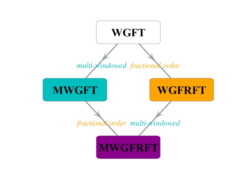
In summary, traditional vertex-frequency analysis methods fail to extract vertex-frequency features in the graph fractional Fourier domain for given window functions. To overcome these limitations, we propose the multi-windowed graph fractional Fourier transform (MWGFRFT), which combines the advantages of multi-window and fractional orders. MWGFRFT is a generalized transform that includes WGFT [17], MWGFT [25], and WGFRFT [34], as illustrated in Fig. 1. With its additional parameters and , MWGFRFT provides enhanced flexibility and adaptability. The main contributions of our work can be summarized as follows:
-
•
Based on the graph fractional translation operator and the graph fractional modulation operator, we obtain a multi-windowed graph fractional Fourier frame (MWGFRFF). Similarly, by applying the graph fractional shift operator and the graph fractional modulation operator, we present a shift multi-windowed graph fractional Fourier frame (SMWGFRFF).
-
•
The MWGFRFT and the shift multi-windowed graph fractional Fourier transform (SMWGFRFT) are defined to obtain a vertex-frequency representation in the graph fractional Fourier domain for given window functions.
-
•
We propose a fast MWGFRFT (FMWGFRFT) algorithm designed to significantly enhance computational efficiency.
-
•
We derive dual frames and tight frames corresponding to MWGFRFF and SMWGFRFF, and also provide a reconstruction formula.
- •
The main connections and differences between the current study and previous ones are concluded as follows:
-
•
These studies focus on vertex-frequency representations, aiming to extract detailed vertex and frequency features.
-
•
WGFT [17], MWGFT [25], and WGFRFT [34] are special cases of the current study. The current study addresses the limitation of WGFT, i.e., its inability to extract detailed vertex or frequency features; The current study overcomes the limitation of MWGFT, which cannot effectively perform frequency feature extraction; The current study resolves the limitation of WGFRFT, i.e., its inability to effectively extract vertex features.
The remaining sections are organized as follows. Section II provides a brief review of the background relevant to this study. In Section III, we define MWGFRFF and present several results related to tight frames and introduce the concept of MWGFRFT. In Section IV, we propose a fast MWGFRFT (FMWGFRFT) algorithm. Section V presents results concerning the dual of MWGFRFF and a reconstruction formula. In Section VI, we define SMWGFRFF and discuss related dual and tight frames. In addition, we introduce the SMWGFRFT concept. In Section VII, the construction of tight MWGFRFF and SMWGFRFF is exemplified. In Section VIII, the experimental results are presented. Section IX presents the applications related to anomaly detection. Finally, Section X concludes this study.
II Preliminaries
II-A Spectral graph theory
An undirected weighted graph consists of a finite set of vertices , where is the number of vertices, is a set of edges and is a weighted adjacency matrix. The non-normalized graph Laplacian is a symmetric difference operator [35], where is a diagonal degree matrix. Suppose that the corresponding Laplacian eigenvalues are arranged in ascending order as: Therefore, where the superscript denotes the Hermitian transpose operation, is a unitary column matrix and is a diagonal matrix.
For a signal defined on the graph , the GFT of is
The inverse GFT is given by
We observe that GFT is represented by the matrix ; as an extension, the spectral graph fractional Fourier transform (SGFRFT) is represented as . The graph fractional Laplacian operator , where [32]. Note that is unitary then is also unitary. And so that for . The SGFRFT of a signal defined on the graph is expressed as [32]:
when , the SGFRFT degenerates into GFT. The inverse SGFRFT is given by
The Parseval relation for the SGFRFT holds. For any signals and defined on the graph , we have
II-B Windowed graph fractional Fourier transform[34]
Definition 1.
(Graph fractional translation operator) For any signal defined on the graph and , the graph fractional translation operator is defined as
| (1) |
Definition 2.
(Graph fractional modulation operator) For any signal defined on the graph and , define the graph fractional modulation operator by
The windowed graph fractional Fourier atoms generated by a window function on are defined by
where and . We denote the set of windowed graph fractional Fourier atoms by
| (2) |
Definition 3.
(Windowed graph fractional Fourier transform) Given a window function , the SGFRFT of is . For a signal , the WGFRFT of is denoted by
II-C Frames and operators[24]
A frame is a collection of vectors that span the signal space, providing a redundant representation of signals. This redundancy can be utilized to facilitate signal reconstruction.
Definition 4.
A family of vectors is a finite frame for if there exist constants such that
holds for every
The constants and are called frame bounds, and if , is called a tight frame. For a tight frame with frame bound , the following reconstruction formula holds:
For a frame , define its synthesis operator by and the analysis operator by Integrating and together, which forms a pair of dual operators, define the frame operator of by , i.e.
which is a positive, bounded, invertible and self-adjoint operator.
If there exists another sequence of vectors such that
then is called a dual frame of
III Multi-windowed graph fractional Fourier frames
In this section, we introduce multi-windowed graph fractional Fourier frames (MWGFRFF) and discuss related tight frames. Furthermore, we define multi-windowed graph fractional Fourier transforms (MWGFRFT).
Analog to (2), for a finite sequence of window functions , the SGFRFT of is , we define the set of multi-windowed graph fractional Fourier atoms by
| (3) |
where
Theorem 1.
Let be the set of multi-windowed graph fractional Fourier atoms defined in (3). If , then is a frame (i.e., MWGFRFF), thus for any signal ,
where lower frame bound
| (4) |
and upper frame bound
| (5) |
Proof.
See Appendix A. ∎
Let where . By Appendix A, Eq. (A) shows that where denotes the entrywise product. Equivalently, we have
| (6) |
where is a diagonal matrix, with its th diagonal entry .
Corollary 1.
is a tight frame if and only if there exists a constant such that for .
Proof.
See Appendix B. ∎
Corollary 2.
Let be the set of multi-windowed graph fractional Fourier atoms defined in (3). If there exists a constant such that for , then is a tight frame with frame bounds
Proof.
See Appendix C. ∎
Definition 5.
(Multi-windowed graph fractional Fourier transform) Given window functions , the SGFRFT of is . Let is a multi-windowed graph fractional Fourier frame defined in Theorem 1. For a signal , the MWGFRFT of is
| (7) |
when , Eq. (7) degenerates into WGFRFT [34]; when , Eq. (7) degenerates into MWGFT [25]; when , Eq. (7) degenerates into WGFT [17].
Proposition 1.
(Diagonal clustering of the vertex-frequency representation with fractional order ) When tends to 0, the vertex-frequency representation of MWGFRFT is clustered on the main diagonal, i.e., all values outside the main diagonal equal to 0.
Proof.
See Appendix D. ∎
IV Fast multi-windowed graph fractional Fourier transform
To improve computational speed, we introduce a fast multi-windowed graph fractional Fourier transform (FMWGFRFT) algorithm. In the classic scenario of signals, the windowed Fourier transform can be calculated through an inverse Fourier transform from the ‘-domain’(the Fourier transform of the windowed Fourier domain)[36]. Applying the idea to graphs [34], we define the -domain as the SGFRFT of MWGFRFT in graph fractional Fourier domain:
| (8) |
Applying (7) to (8), similar to [34], then we get
where .
Definition 6.
(Fast multi-windowed graph fractional Fourier transform). The inverse SGFRFT of on the variable is FMWGFRFT, i.e.,
The calculation algorithm of FMWGFRFT is defined as follows:
(i) The loop about for . This step has computational complexity.
(ii) Calculate by using matrices:
where represents Hadamard multiplication and denotes the standard matrix multiplication. Each row of is the signal , and denotes the complex conjugate of the graph fractional basis . This step has computational complexity.
(iii) Form a matrix such that each row is the SGFRFT of a window function .
This step does not influence the computational complexity.
(iv) Calculate the -domain representation.
The computational complexity is .
(v) The vertex-frequency content is obtained by applying inverse SGFRFT to each row of ,i.e.
where denotes the non-conjugate transpose of . The complexity of this step is
(vi) Perform matrix addition on these matrices. The complexity of this step is
To sum up, the computational complexity of FWGFRFT is . As increases, this computational complexity is a significant improvement, compared with MWGFRFT algorithm and MWGFT [25] algorithm which have the computational complexity of .
V Dual of multi-windowed graph fractional Fourier frames
In this section, we obtain a reconstruction formula by introducing the dual of multi-windowed graph fractional Fourier frames. In addition, the canonical dual is also introduced.
Let denote the set of multi-windowed graph fractional Fourier atoms, generated by a finite sequence of window functions in the sense of (3). is called a dual to if for any , there exists a constant such that
| (9) |
Theorem 2.
Suppose that is multi-windowed graph fractional Fourier frame as defined in (3). If there exists a finite sequence of window functions and a constant such that
then is a dual of .
Proof.
See Appendix E. ∎
We could also prove that the dual of a multi-windowed graph fractional Fourier frame is also a frame.
Corollary 3.
Suppose that is a multi-windowed graph fractional Fourier frame as defined in (3). If there exists a finite sequence of window functions and a constant such that for , then is also a multi-windowed graph fractional Fourier frame.
Proof.
See Appendix F. ∎
Corollary 4.
Suppose that is a multi-windowed graph fractional Fourier frame as defined in (3). Let be a vector with and be a vector with for . Then the canonical dual frame of is given by
where ; ; ; .
Proof.
See Appendix G. ∎
VI Shift multi-windowed graph fractional Fourier frames
In GSP, the adjacency matrix acts as a shift operator [1]. In graph fractional Fourier domain, different fractional shift operators are proposed [37, 38, 39]. Assume that the eigen-decomposition of the graph adjacency matrix is , in this paper, define the graph fractional shift operator as
to facilitate the construction of tight frames in Section VII later. Then we could design a new type of frames and introduce the concept of shift multi-windowed graph fractional Fourier transform (SMWGFRFT).
Theorem 3.
Given window vectors with for . Define where denotes the Hadamard product. Also define
| (10) |
where is the th row of matrix and . The set of shift multi-window graph fractional Fourier atoms
| (11) |
forms a frame (i.e., SMWGFRFF) for signals defined on if and only if for all of elements of . The optimal lower and upper frame bounds are
| (12) |
respectively.
Proof.
See Appendix H. ∎
Corollary 5.
Suppose that is a shift multi-windowed graph fractional Fourier frame as defined in (11). Let be a vector with and be a vector with for Then the canonical dual frame of is defined as where .
Proof.
The proof is similar to Corollary 4. ∎
Corollary 6.
Let be a shift multi-windowed graph fractional Fourier frame and is the th row of matrix . is a tight frame if and only if for where C is a constant number and .
Proof.
See Appendix I. ∎
It is known that , where is the th row of matrix . Then we define , where denotes the non-conjugate transpose of . Given window functions , we can define a new set of shift multi-windowed graph fractional Fourier atoms by
| (13) |
where
Definition 7.
(Shift multi-windowed graph fractional Fourier transform) Given window functions , let is a shift multi-windowed graph fractional Fourier frame defined in (13). For a graph signal , the SMWGFRFT of is denoted by
It is apparently that the computational complexity of SMWGFRFT is .
VII Two types of tight multi-windowed graph fractional Fourier frames
In this section, we design tight multi-windowed graph fractional Fourier frames(TMWGFRFF) and tight shift multi-windowed graph fractional Fourier frames (TSMWGFRFF).
VII-A Construction of TMWGFRFF
Constructing tight MWGFRFF is equivalent to find window functions such that for By Corollary 2, the goal of the construction is to find a sequence of window functions such that for , where denotes graph fractional Laplacian spectrum. Among the functions with such a property, we think of the cardinal B-spline as a candidate.
The th order cardinal B-spline is defined as follows:
The integer-translates of the th order cardinal B-spline form a partition of unity, i.e.,
| (14) |
Suppose that the normalized graph fractional Laplacian matrix is applied, that is, the corresponding graph fractional Laplacian spectrum is contained in [0, 2]. We then take B-spline to construct the tight frame window functions:
Letting , , and = , according to Eq. (14), we have That is, is a set of tight frame window functions.
VII-B Construction of TSMWGFRFF
When the rows of the graph fractional shift operator have identical 2-norm, we could construct orthonormal vectors as the tight SMWGFRFF:
(i) the graph fractional Laplacian eigenvectors, i.e. for , where is the th eigenvector of the graph fractional Laplacian matrix.
(ii) Householder vectors with localized generator, i.e. , where is the th vector of the Householder matrix and is a vector localized on a small set of indices.
VIII Experiments
We conduct several simulations by using frame, dual frame, and tight frame window functions to evaluate the effectiveness of MWGFRFT, FMWGFRFT, and SMWGFRFT in extracting the vertex-frequency features of graph signals. Our methods are also compared with WGFT[17], MWGFT[25] and WGFRFT[34].
VIII-A Comparative Analysis of Vertex-Frequency Feature Extraction among WGFT[17], MWGFT[25], WGFRFT[34] and MWGFRFT
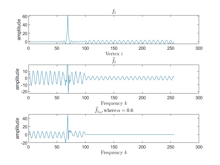
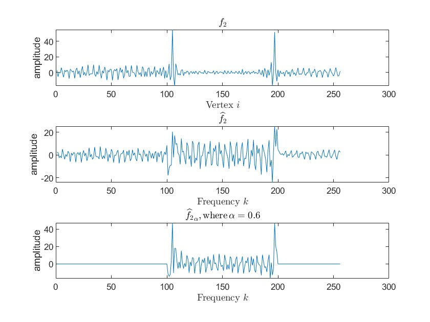
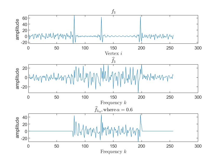
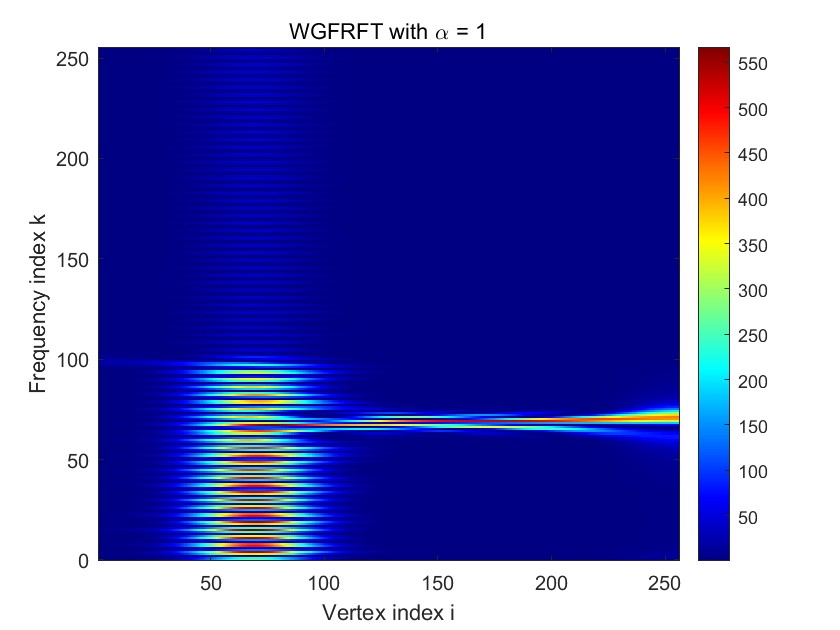
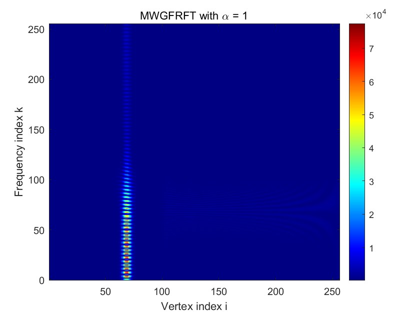
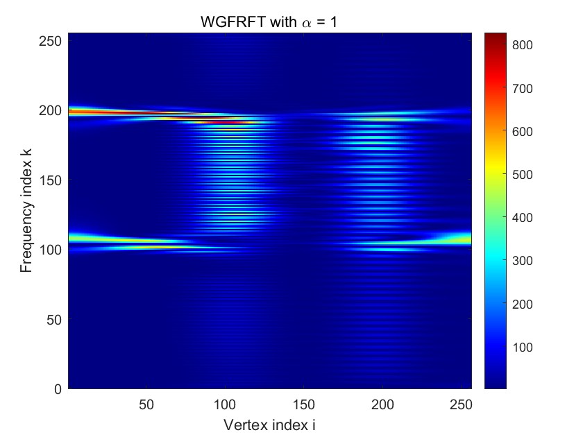
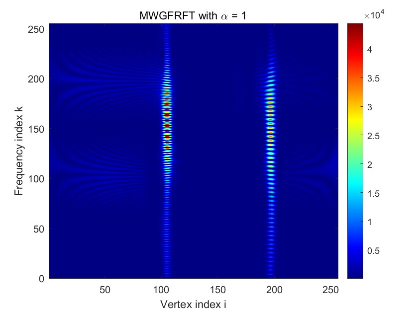
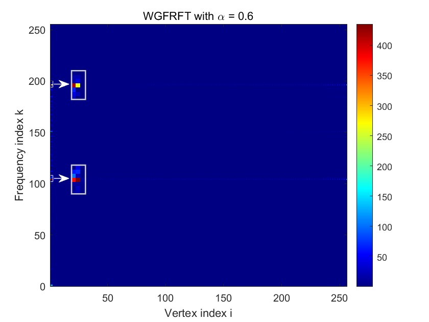
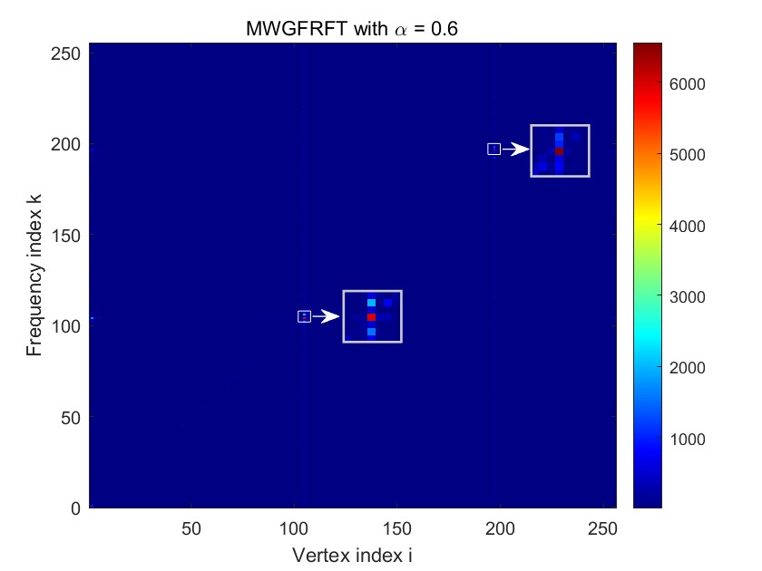
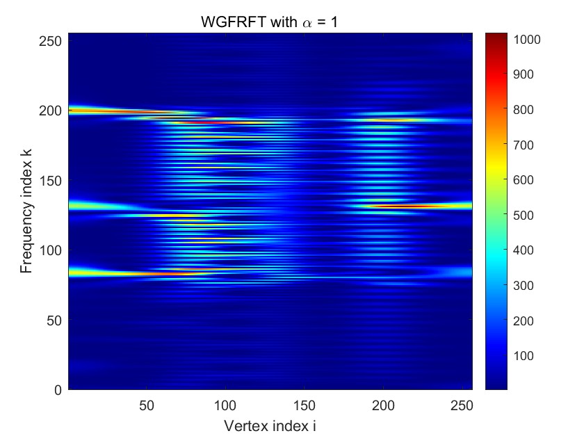
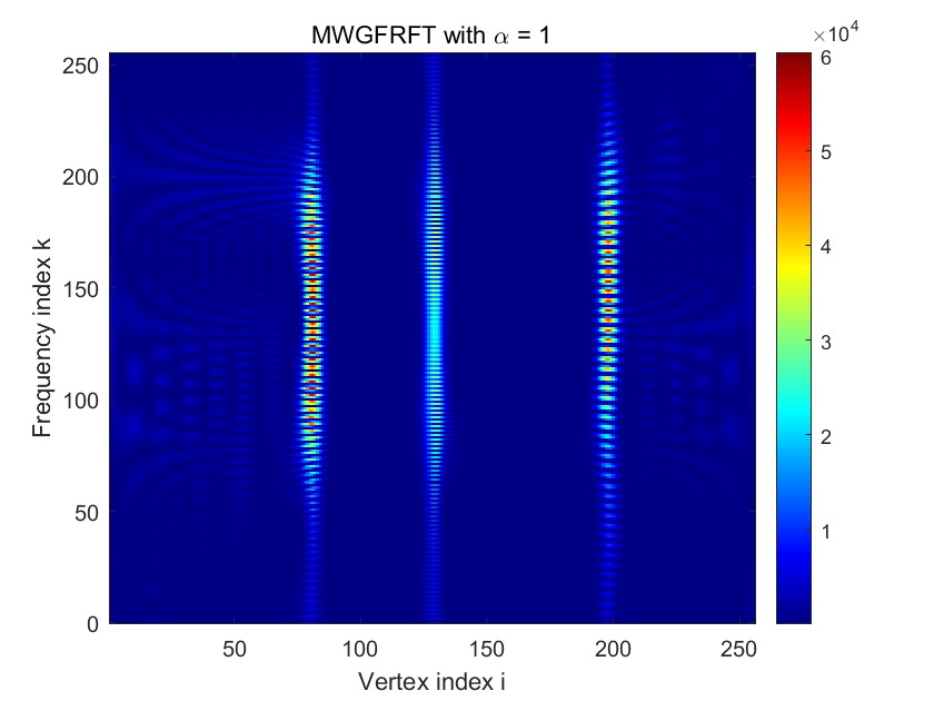
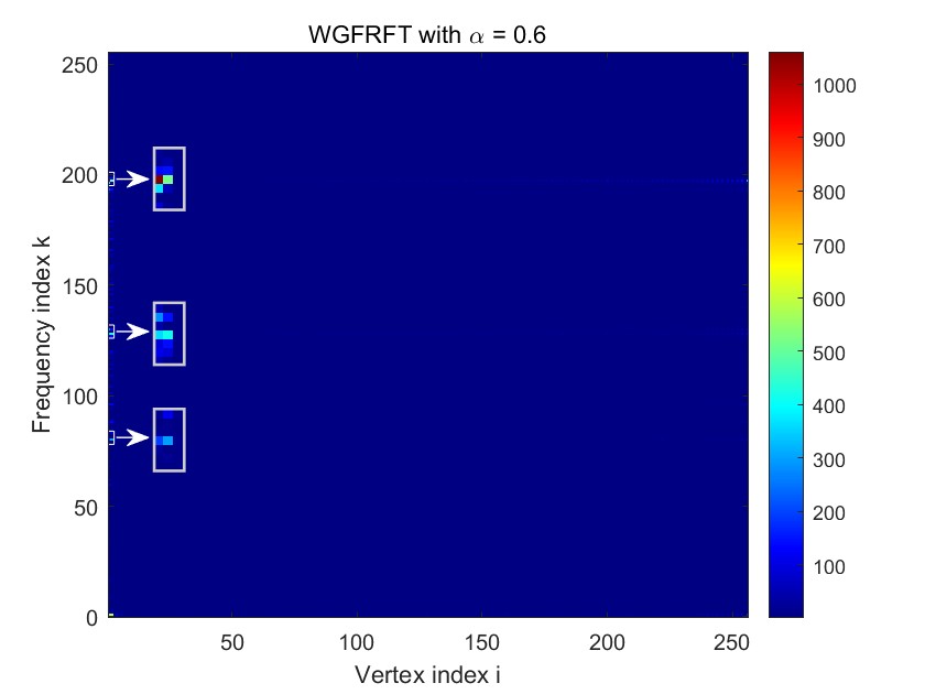
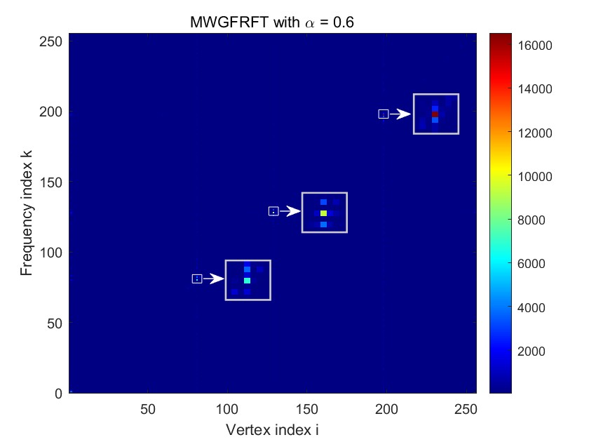
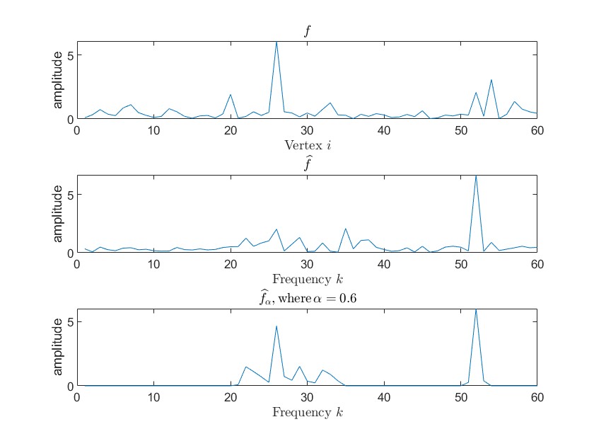
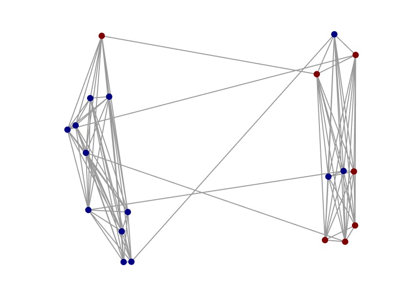
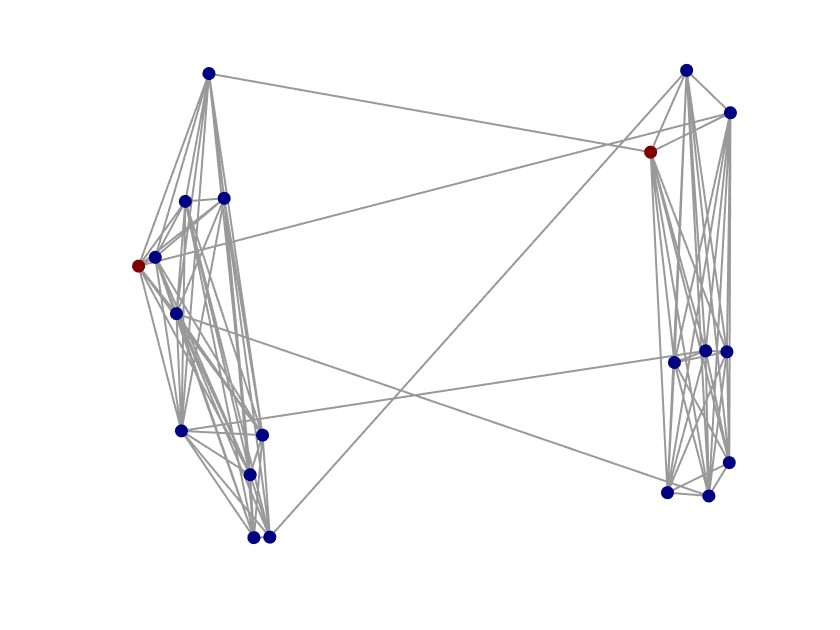
First, we consider a path graph with 256 vertices, all of which have equal weights of 1. The eigenvectors of the graph Laplacian are generated from the basis vectors of the DCT-II transform. We consider the following three signals in Fig. 2: is a band limited signal in graph fractional Fourier domain, and are bandpass signals in graph fractional Fourier domain. We choose the heat diffusion kernel as the window function by setting with and choosing such that . Applying Eq.(1) to , then obtain windows. The “spectrograms” in Fig. 3 show for all and .
From Fig. 3, the vertex-frequency features of the three signals are clearly observed using MWGFRFT, enabling precise identification of the brightest points by combining their vertex and frequency information. However, none of WGFT, MWGFT and WGFRFT can accurately extract the vertex-frequency features of the three signals. The vertex domain features of the three signals by WGFT are unclear and cannot be accurately determined. For MWGFT, the vertex domain features of the 3 signals are clearly determined, however, the corresponding frequency features at each vertex cannot be accurately localized, nor can the location of the brightest point in the spectrograms be determined. For WGFRFT, no accurate vertex features are identified, and all frequency features are located at the smallest vertices .
VIII-B Algorithm evaluation of FMWGFRFT
To evaluate the performance of FMWGFRFT algorithm, we conducted experiments to demonstrate its effectiveness and robustness.
(i) effectiveness
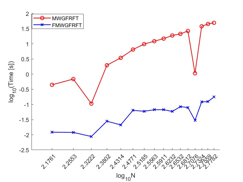
To clearly demonstrate the temporal advantage of the fast algorithm, we compare the time cost of the fast algorithm (FMWGFRFT) with the original algorithm (MWGFRFT). Setting the fractional order , we contemplate a random ring graph with different number of vertices , where the signal is . We choose the standard Gaussian function as the window function , applying Eq.(1) to , and then obtain windows. In Fig. 4, the x-axis represents the logarithm of the number of vertices and the y-axis represents the logarithm of computation time (in seconds). For MWGFRFT, the red line corresponds to a linear fit, aligning with the theoretical computational complexity of . Similarly, for FMWGFRFT, the blue line corresponds to a linear fit, which matches the theoretical computational complexity of . The results indicate that FMWGFRFT is more efficient and requires less computation time compared to MWGFRFT.
(ii) Robustness
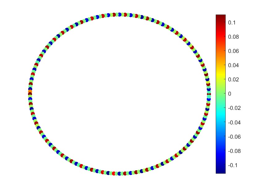
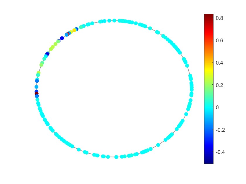
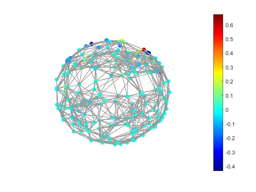
In the first experiment, we simulate with 3 graphs of 200 vertices: a ring graph, a random ring graph and a sphere graph. We take the real parts of the 3 graph signals as follows.
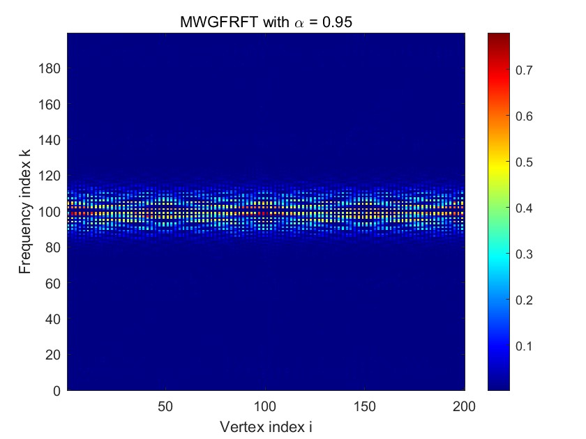
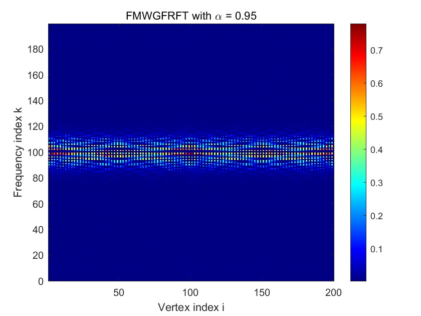
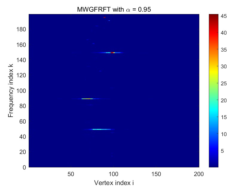
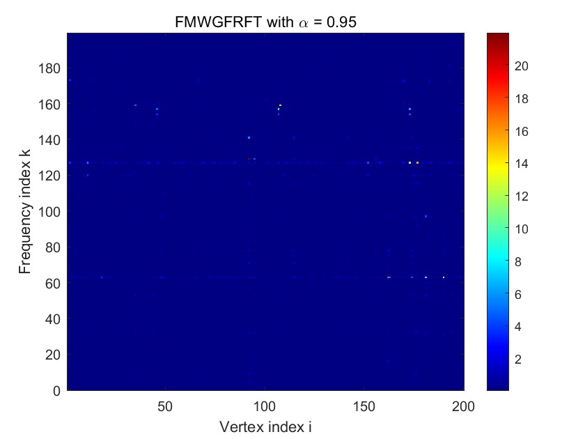
For fixed , we take and from the fractional Laplacian matrix of a ring graph, a random ring graph and a sphere graph, respectively. The details of the original signals are shown in Fig. 5(a),(d),(g). We choose the heat diffusion kernel as the window function . In Fig. 5, we note that the details of the spectrograms by MWGFRFT and FMWGFRFT are the same. Moreover, we can observe that the vertex-frequency representations of FMWGFRFT closely match that of MWGFRFT for the 3 signals; moreover, FMWGFRFT effectively identified the correct frequencies, further validating the correctness and effectiveness of FMWGFRFT algorithm.


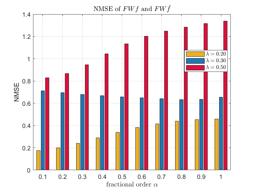
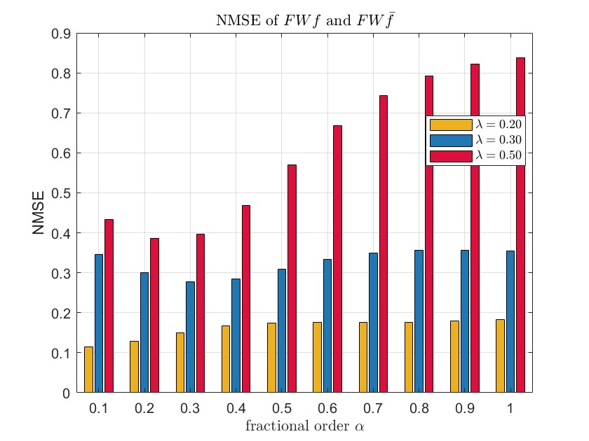
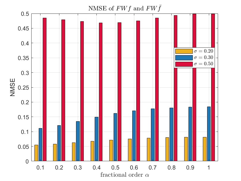
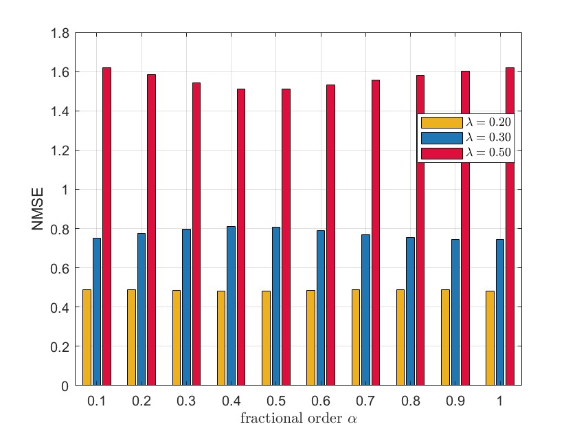
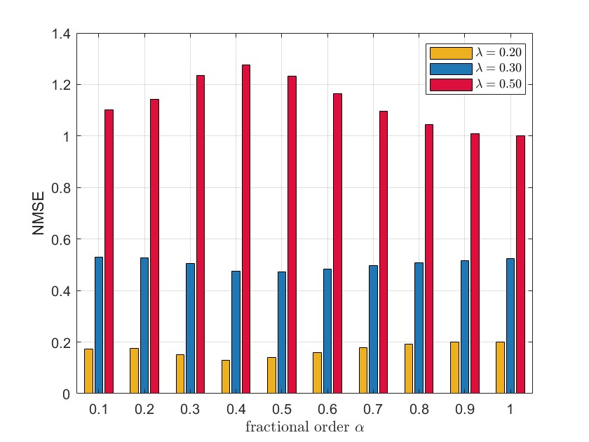
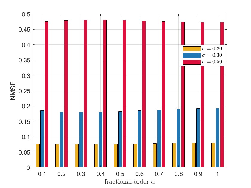
In the second experiment, we vary both the fractional order and the noise parameter. The normalized mean squared error (NMSE) is computed between the FMWGFRFT coefficients of 3 original signals and their corresponding contaminated signals, as illustrated in Fig. 6. In Fig. 7, the WGFRFT results are presented by using a single window function, while all other conditions remain identical to those in Fig. 6.
We experiment with 3 graphs of vertices: for the sphere graph, we add Poisson noise with parameter , , and to signal ; for the community graph, we add exponential noise with parameter , , and to signal ; for the swiss roll graph, we add Gaussian noise with standard deviation , , and to signal , respectively.
For the original signals , and , the contaminated signals are denoted by , and . We choose the standard Gaussian function as the window function by setting with and choosing such that . Applying Eq. (1) to , and then obtain windows. We then calculate the normalized mean squared error (NMSE) between the transform coefficients of the original signal and the contaminated signal, which is given by:
where , is the number of vertices, and are the FWGFRFT coefficients of the original and contaminated signals, respectively.
From Fig. 6 and Fig. 7, we observe that, despite differences in graph structure and noise, a higher noise parameter corresponds to a larger value of NMSE. Compared to WGFT, MWGFT and WGFRFT, the FMWGFRFT algorithm consistently achieves the lower NMSE, highlighting its robustness and reliability across diverse scenarios. To minimize the value of NMSE, an appropriate choice of fractional order can be chosen depending on the specific case.
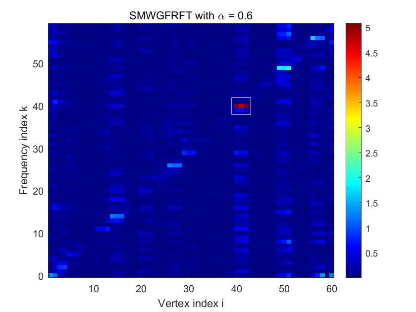
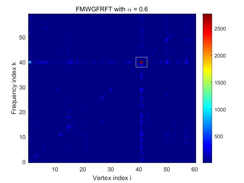
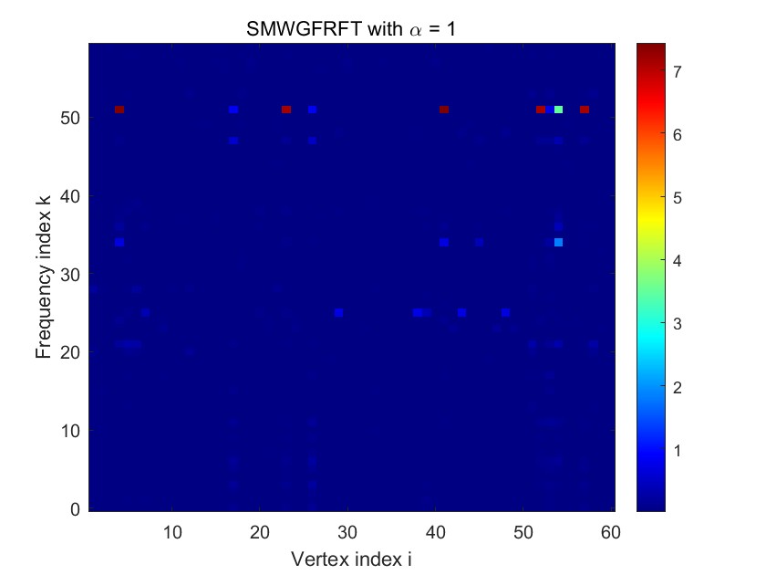
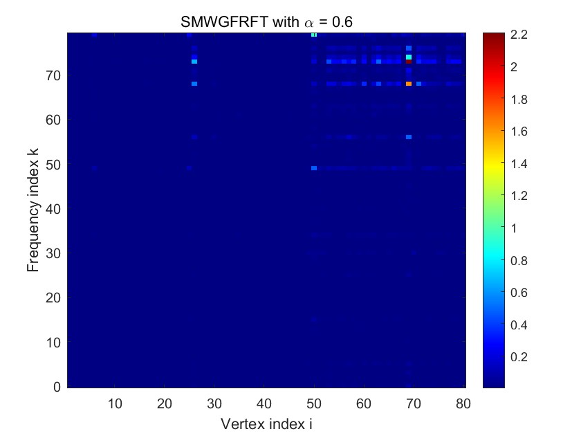
VIII-C Examples of SMWGFRFT and FMWGFRFT
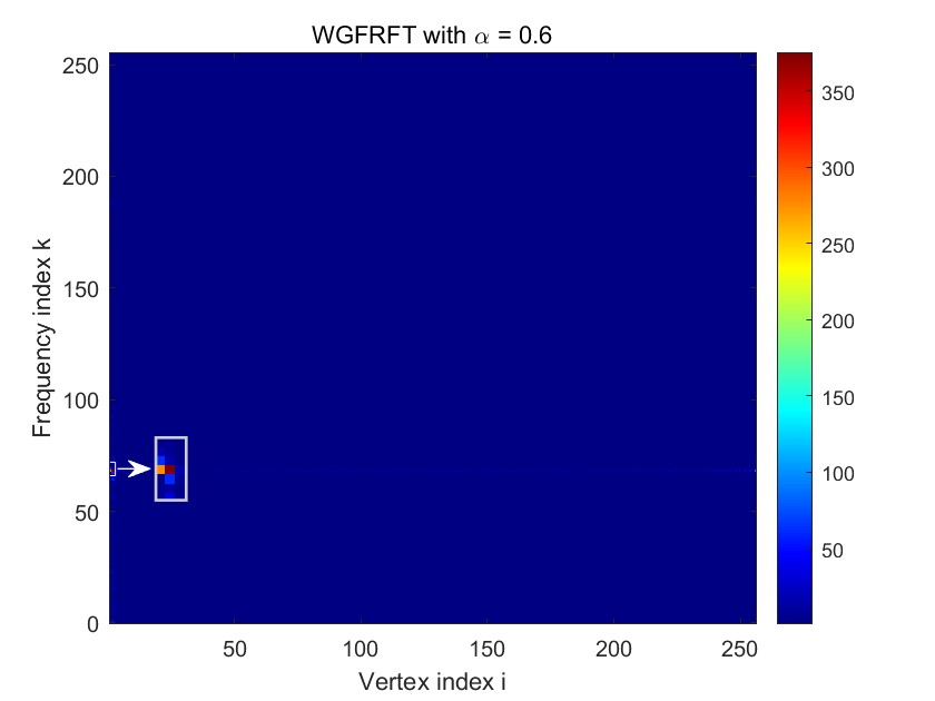
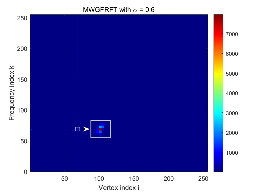
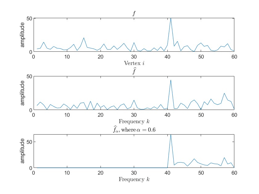
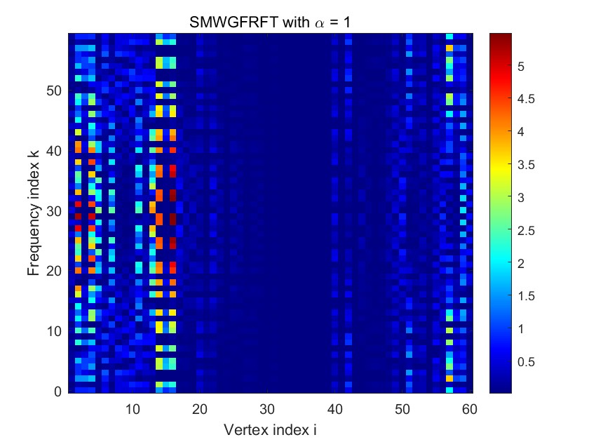
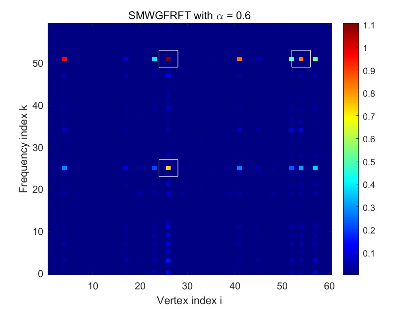
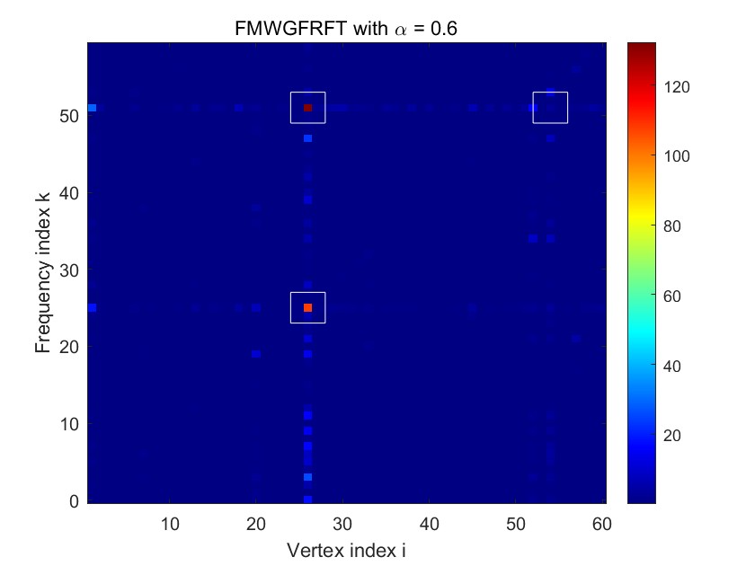
First, we analyze two distinct graph structures: a ring graph with 60 vertices paired with the signal , and a Swiss roll graph with 60 vertices paired with the signal . We choose the heat diffusion kernel as the window function by setting with and choosing such that . Applying Eq.(1) to , and then obtain windows. From Fig. 8, we know that SMWGFT fails to identify vertex or frequency information, overlooking key vertex-frequency features. Comparing Fig. 8(c) and Fig. 8(d), we observe that FMWGFRFT effectively identifies vertex-frequency features. In contrast, while SMWGFRFT demonstrates proficiency in capturing vertex-frequency features, it misidentifies certain vertices. By comparing Fig. 8(g) with Fig. 8(h), we observe that FMWGFRFT identifies only the prominent vertex-frequency features, disregarding those with less distinct features. In contrast, SMWGFRFT captures all vertex-frequency features but introduces some errors in identifying certain points. Therefore, SMWGFRFT and FMWGFRFT can complement each other in identifying vertex-frequency features and are best utilized in combination.
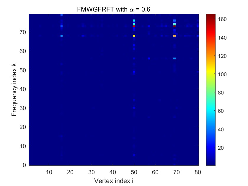
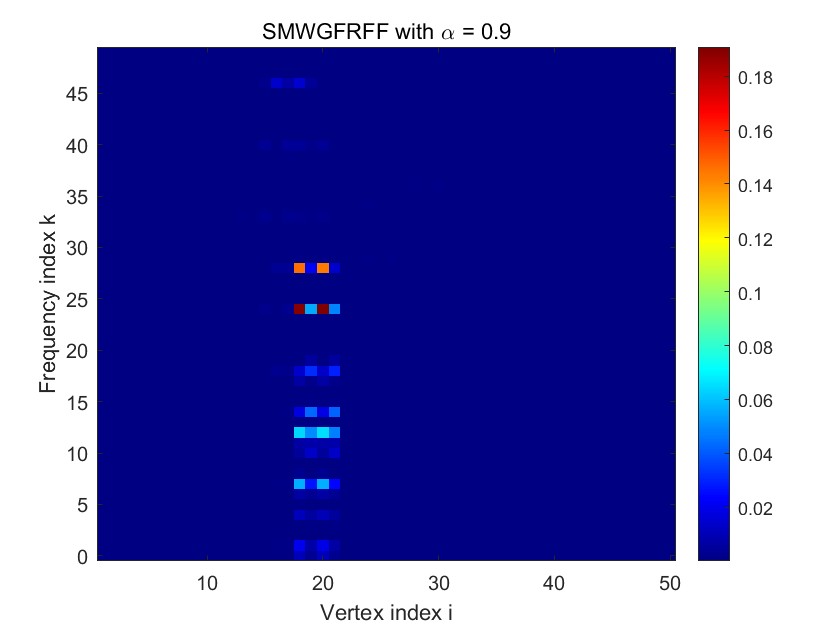
Second, we analyze a community graph with 80 vertices and the signal . We choose the dual heat diffusion kernel as the window function by setting with and , choosing such that . Applying Eq.(1) to , and then obtain windows. In Fig. 9, the spectrograms are generated by using dual FMWGFRFT and dual SMWGFRFT with . Fig. 9 demonstrates that both dual FMWGFRFT and dual SMWGFRFT are capable of extracting vertex-frequency features.
Thirdly, we consider a random ring graph with 50 vertices and the signal in Fig. 10. The FMWGFRFF window functions is derived from B-spline by Section VII-A. The SMWGFRFF window functions is given by the Householder matrix. By Section VII-B(ii), the Householder matrix is obtained, where
Fig. 10 demonstrates that both tight FMWGFRFT and Householder tight SMWGFRFT are capable of extracting vertex-frequency features.
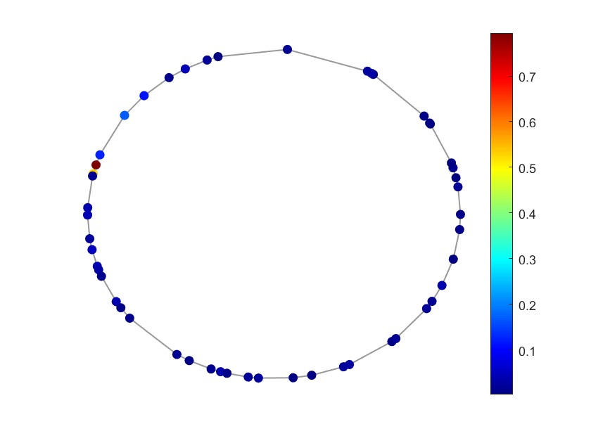

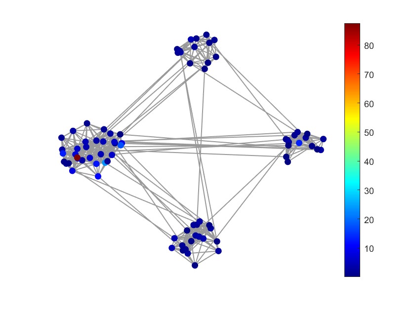
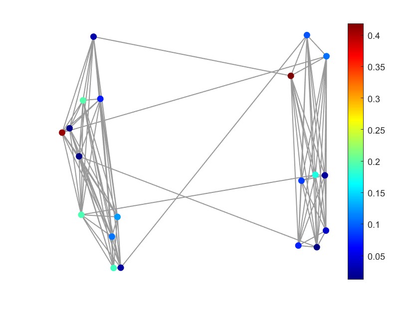
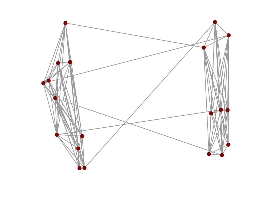
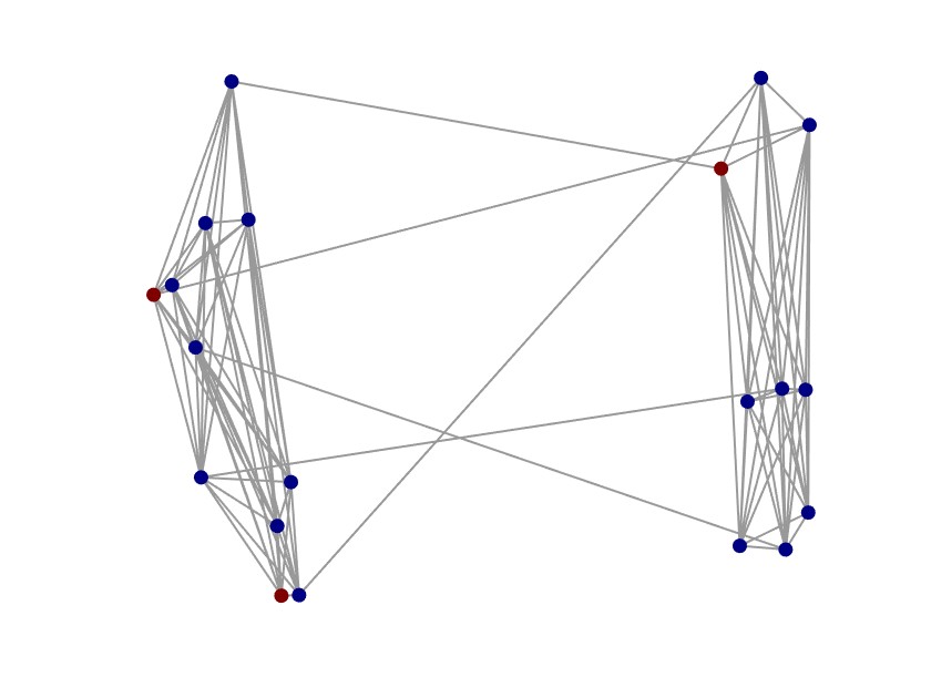
IX Applications: anomaly detection
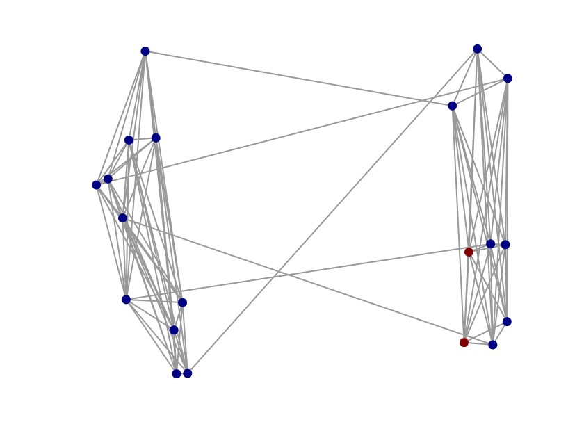
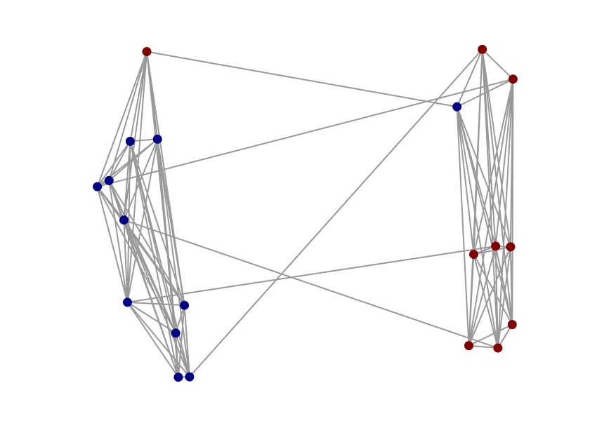
In graph fractional Fourier domain, WGFT [17], MWGFT [25], WGFRFT [34], SMWGFT, SMWGFRFT and FMWGFRFT are applied to detect anomaly signals. The test involves an anomaly signal in Fig.11(a), characterized by two anomalous deep red vertices, on a community graph with 20 vertices. The spectrograms are computed by using WGFT [17], MWGFT [25], WGFRFT [34], SMWGFT, SMWGFRFT and FMWGFRFT. Taking maximum of with respect to the vertices, the spectrogram coefficient threshold is defined as , where represents the spectrogram coefficient. Vertices with maximum spectrogram coefficients exceeding are highlighted in red. In Fig.11(b), the WGFT spectrogram detects all vertices as anomalies. In Fig.11(c), the MWGFT spectrogram identifies all anomalous vertices but incorrectly classifies one additional vertex as anomalous. In Fig. 11(d), the WGFRFT spectrogram fails to detect the anomalous vertices. In Fig.11(e), the SMWGFT spectrogram also fails to detect the anomalous vertices. In Fig.11(f), the SMWGFRFT spectrogram identifies one anomaly vertex but incorrectly classifies too many vertices as anomalous. In Fig. 11(g), the FMWGFRFT spectrogram successfully detects all anomalous vertices. This example highlights the effectiveness of FMWGFRFT in accurately identifying the vertices associated with the anomaly signals.
X Conclusion
By performing a comparative analysis of vertex-frequency feature extraction among WGFT [17], WGFRFT [34], MWGFT [25], and MWGFRFT, it becomes evident that MWGFRFT offers significant advantages in vertex-frequency representation in the graph fractional Fourier domain for given window functions. The performance of MWGFRFT and FMWGFRFT is compared with regard to vertex-frequency representation, normalized mean squared error, and time cost. The experimental results demonstrate the robustness and effectiveness of the FMWGFRFF algorithm. Experiments with SMWGFRFT and FMWGFRFT on different graphs demonstrate that SMWGFRFT and FMWGFRFT effectively extract vertex-frequency features. Furthermore, SMWGFRFT and FMWGFRFT are mutually complementary in identifying vertex-frequency features and are most effective when utilized in tandem. Additionally, dual and tight frame window functions have demonstrated effectiveness in extracting vertex-frequency features. In the graph fractional domain, FMWGFRFT demonstrates effectiveness in accurately detecting anomaly signals.
Appendix A Proof of Theorem 1
Appendix B Proof of Corollary 1
From (6), the frame operator of can be written as the diagonal matrix with for . Note that the optimal lower and upper frame bounds of a frame are the smallest and largest eigenvalues of the frame operator, respectively [24], the frame bounds of are given by the smallest and largest entries in . Therefore, is a tight frame if and only if is a constant vector; that is, there exists a constant such that for .
Appendix C Proof of Corollary 2
Appendix D Proof of Proposition 1
The proofs of FMWGFRFT, MWGFRFT, MWGFT[25], WGFRFT[34] and WGFT[17] are analogous. For the sake of convenience, we will only provide the proof for FMWGFRFT. Note that the FMWGFRFT matrix
As we all know, when tends to 0, the graph fractional Fourier basis matrix tends to the identity matrix, i.e., . Then we have
We know that as tends to 0, the vertex-frequency representation of FMWGFRFT is clustered on the main diagonal, i.e., all values outside the main diagonal equal to 0.
Appendix E Proof of Theorem 2
Appendix F Proof of Corollary 3
If for , by the Cauchy-Schwartz inequality, we have
Then and for . By Theorem 1,we have is also a multi-windowed graph fractional Fourier frame.
Appendix G Proof of Corollary 4
Suppose that is the frame operator of . In the proof of Corollary 1, we have that According to the definitions of frame and operator, the canonical frame of is then given by
Appendix H Proof of Theorem 3
We have
where . Let , the corresponding synthesis operator of can be expressed as . We know that forms a frame if and only if its frame operator is positive definite. In fact, the frame operator of can be expressed as
Here is an identity matrix. Let , we have
Let is the th row of matrix , the th diagonal entry of can be written as . Therefore, is a frame if and only if for . The frame bounds of are given by (12) which are the smallest and largest elements of .
Appendix I Proof of Corollary 6
By Theorem 3, the frame bounds of are given by the smallest and largest elements in , with . Hence, is a tight frame is then equivalent to the condition that for .
References
- [1] A. Sandryhaila and J. M. Moura, “Big data analysis with signal processing on graphs: Representation and processing of massive data sets with irregular structure,” IEEE Signal Process. Mag., vol. 31, no. 5, pp. 80–90, 2014.
- [2] L. Stanković and E. Sejdić, Vertex-frequency Analysis of Graph Signals. Springer, 2019.
- [3] A. Ortega, P. Frossard, J. Kovačević, J. M. Moura, and P. Vandergheynst, “Graph signal processing: Overview, challenges, and applications,” Proc. IEEE, vol. 106, no. 5, pp. 808–828, 2018.
- [4] A. Sandryhaila and J. M. Moura, “Discrete signal processing on graphs: Frequency analysis,” IEEE Trans. Signal Process., vol. 62, no. 12, pp. 3042–3054, 2014.
- [5] E. Ceci and S. Barbarossa, “Graph signal processing in the presence of topology uncertainties,” IEEE Trans. Signal Process., vol. 68, pp. 1558–1573, 2020.
- [6] F. Gama, E. Isufi, G. Leus, and A. Ribeiro, “Graphs, convolutions, and neural networks: From graph filters to graph neural networks,” IEEE Signal Process. Mag., vol. 37, no. 6, pp. 128–138, 2020.
- [7] M. W. Morency and G. Leus, “Graphon filters: Graph signal processing in the limit,” IEEE Trans. Signal Process., vol. 69, pp. 1740–1754, 2021.
- [8] G. Leus, A. G. Marques, J. M. Moura, A. Ortega, and D. I. Shuman, “Graph signal processing: History, development, impact, and outlook,” IEEE Signal Process. Mag., vol. 40, no. 4, pp. 49–60, 2023.
- [9] J. Domingos and J. M. Moura, “Graph Fourier transform: A stable approximation,” IEEE Trans. Signal Process., vol. 68, pp. 4422–4437, 2020.
- [10] J. Jiang, C. Cheng, and Q. Sun, “Nonsubsampled graph filter banks: theory and distributed algorithms,” IEEE Trans. Signal Process., vol. 67, no. 15, pp. 3938–3953, 2019.
- [11] J. Jiang, D. B. Tay, Q. Sun, and S. Ouyang, “Design of nonsubsampled graph filter banks via lifting schemes,” IEEE Signal Process. Lett., vol. 27, pp. 441–445, 2020.
- [12] S. Chen, R. Varma, A. Sandryhaila, and J. Kovačević, “Discrete signal processing on graphs: Sampling theory,” IEEE Trans. Signal Process., vol. 63, no. 24, pp. 6510–6523, 2015.
- [13] S. Chen, A. Sandryhaila, J. M. Moura, and J. Kovačević, “Signal recovery on graphs: Variation minimization,” IEEE Trans. Signal Process., vol. 63, no. 17, pp. 4609–4624, 2015.
- [14] I. Jestrović, J. L. Coyle, and E. Sejdić, “A fast algorithm for vertex-frequency representations of signals on graphs,” Signal Process., vol. 131, pp. 483–491, 2017.
- [15] L. Le Magoarou and R. Gribonval, “Are there approximate fast Fourier transforms on graphs?” in Proc. IEEE Int. Conf. Acoust., Speech Signal Process. (ICASSP). IEEE, 2016, pp. 4811–4815.
- [16] L. Le Magoarou, R. Gribonval, and N. Tremblay, “Approximate fast graph Fourier transforms via multilayer sparse approximations,” IEEE Trans. Signal Inf. Process. Netw., vol. 4, no. 2, pp. 407–420, 2017.
- [17] D. I. Shuman, B. Ricaud, and P. Vandergheynst, “Vertex-frequency analysis on graphs,” Appl. Comput. Harmon. Anal., vol. 40, no. 2, pp. 260–291, 2016.
- [18] ——, “A windowed graph Fourier transform,” in Proc. IEEE Statist. Signal Process. Workshop (SSP). IEEE, 2012, pp. 133–136.
- [19] N. Linh-Trung, N. V. Dung, K. Abed-Meraim et al., “A new windowed graph Fourier transform,” in Proc. NAFOSTED Conference on Information and Computer Science (NICS). IEEE, 2017, pp. 150–155.
- [20] R. Shafipour, A. Khodabakhsh, and G. Mateos, “A windowed digraph Fourier transform,” in Proc. IEEE Int. Conf. Acoust., Speech Signal Process. (ICASSP). IEEE, 2019, pp. 7525–7529.
- [21] H. Rabiei, F. Richard, M. Roth, J.-L. Anton, O. Coulon, and J. Lefèvre, “The graph windowed Fourier transform: a tool to quantify the gyrification of the cerebral cortex,” in Workshop on Spectral Analysis in Medical Imaging (SAMI), 2015.
- [22] Y. Liu, F. Zhang, H. Miao, and R. Tao, “The hopping discrete fractional Fourier transform,” Signal Process., vol. 178, p. 107763, 2021.
- [23] L. Stanković, D. Mandic, M. Daković, B. Scalzo, M. Brajović, E. Sejdić, and A. G. Constantinides, “Vertex-frequency graph signal processing: A comprehensive review,” Digit. Signal Process., vol. 107, p. 102802, 2020.
- [24] P. G. Casazza and G. Kutyniok, Finite Frames: Theory and Applications. Springer Science & Business Media, 2012.
- [25] X. Zheng, C. Zou, L. Dong, and J. Zhou, “Multi-windowed vertex-frequency analysis for signals on undirected graphs,” Comput. Commun., vol. 172, pp. 35–44, 2021.
- [26] J. J. Healy, M. A. Kutay, H. M. Ozaktas, and J. T. Sheridan, Linear Canonical Transforms: Theory and Applications. Springer, 2015, vol. 198.
- [27] R. Tao, Y.-L. Li, and Y. Wang, “Short-time fractional Fourier transform and its applications,” IEEE Trans. Signal Process., vol. 58, no. 5, pp. 2568–2580, 2009.
- [28] R. Tao, B.-Z. Li, and Y. Wang, “Spectral analysis and reconstruction for periodic nonuniformly sampled signals in fractional Fourier domain,” IEEE Trans. Signal Process., vol. 55, no. 7, pp. 3541–3547, 2007.
- [29] L. Stanković, T. Alieva, and M. J. Bastiaans, “Time–frequency signal analysis based on the windowed fractional Fourier transform,” Signal Process., vol. 83, no. 11, pp. 2459–2468, 2003.
- [30] Y.-Q. Wang, B.-Z. Li, and Q.-Y. Cheng, “The fractional Fourier transform on graphs,” in Proc. Asia-Pacific Signal and Information Processing Association Annual Summit and Conference (APSIPA ASC). IEEE, 2017, pp. 105–110.
- [31] Y. Wang and B. Li, “The fractional Fourier transform on graphs: Sampling and recovery,” in Proc. IEEE International Conference on Signal Processing (ICSP). IEEE, 2018, pp. 1103–1108.
- [32] J. Wu, F. Wu, Q. Yang, Y. Zhang, X. Liu, Y. Kong, L. Senhadji, and H. Shu, “Fractional spectral graph wavelets and their applications,” Math. Probl. Eng., vol. 2020, no. 1, p. 2568179, 2020.
- [33] T. Alikaşifoğlu, B. Kartal, and A. Koç, “Graph fractional Fourier transform: A unified theory,” IEEE Trans. Signal Process., vol. 72, pp. 3834–3850, 2024.
- [34] F.-J. Yan and B.-Z. Li, “Windowed fractional Fourier transform on graphs: Properties and fast algorithm,” Digit. Signal Process., vol. 118, p. 103210, 2021.
- [35] D. I. Shuman, S. K. Narang, P. Frossard, A. Ortega, and P. Vandergheynst, “The emerging field of signal processing on graphs: Extending high-dimensional data analysis to networks and other irregular domains,” IEEE Signal Process. Mag., vol. 30, no. 3, pp. 83–98, 2013.
- [36] R. A. Brown, M. L. Lauzon, and R. Frayne, “A general description of linear time-frequency transforms and formulation of a fast, invertible transform that samples the continuous s-transform spectrum nonredundantly,” IEEE Trans. Signal Process., vol. 58, no. 1, pp. 281–290, 2009.
- [37] Z. Yan and Y. Deng, “Single node reconstruction of graph signal based on graph fractional Fourier transform,” in Proc. International Conference on Signal Image Processing and Communication (ICSIPC), vol. 12246. SPIE, 2022, pp. 133–138.
- [38] F.-J. Yan and B.-Z. Li, “A new reconstruction formula and shift frame for WGFRFT,” in Proc. International Conference on Signal Image Processing and Communication (ICSIPC), vol. 12916. SPIE, 2023, pp. 267–273.
- [39] G. B. Ribeiro, J. R. D. O. Neto, and J. B. Lima, “On the fractionalization of the shift operator on graphs,” IEEE Access, vol. 10, pp. 16 468–16 478, 2022.